GLA-Net: An Attention Network with Guided Loss for Mismatch Removal

Abstract

Mismatch removal is a critical prerequisite in many feature-based tasks. Recent attempts cast the mismatch removal task as a binary classification problem and solve it through deep learning based methods. In these methods, the imbalance between positive and negative classes is important, which affects network performance, i.e., Fn-score. To establish the link between Fn-score and loss, we propose to guide the loss with the Fn-score directly. We theoretically demonstrate the direct link between our Guided Loss and Fn-score during training. Moreover, we discover that outliers often impair global context in mismatch removal networks. To address this issue, we introduce the attention mechanism to mismatch removal task and propose a novel Inlier Attention Block (IA Block). To evaluate the effectiveness of our loss and IA Block, we design an end-to-end network for mismatch removal, called GLA-Net . Experiments have shown that our network achieves the state-of-the-art performance on benchmark datasets.

Introduction

Establishing stable and abundant feature matches between overlapping image pairs is a fundamental component of many tasks in computer vision, such as Structure from Motion (SfM) (?), simultaneous localization and mapping (SLAM) (?) and so on. Due to the ambiguity of local texture information, the matching results often contain a large number of mismatches. Recently, some methods (?) adopt deep learning for mismatch removal. Specifically, they first obtain massive putative feature correspondences through hand-crafted local feature descriptors with loose matching conditions, such as SIFT (?). Then the putative set is divided into positives (inliers) and negatives (outliers) through a trainable deep learning network. The positive class of network classification is considered as the final matching result.

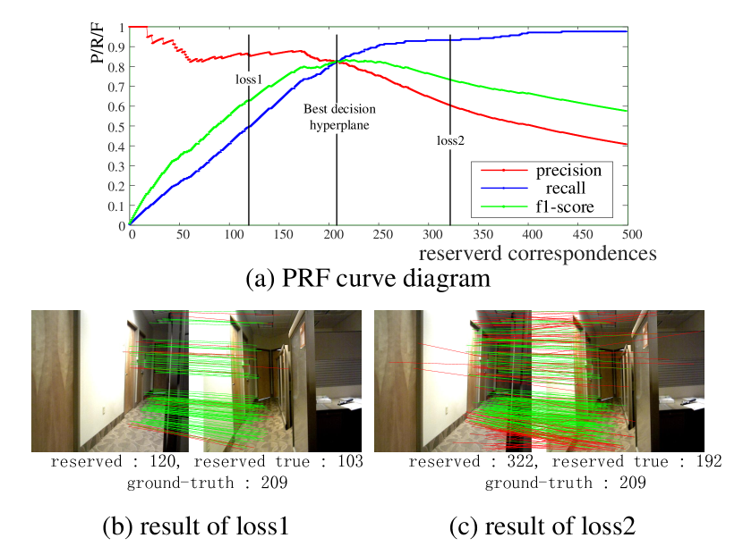
Figure 1: The top (a) is the curve diagram of the reserved correspondences and PRF, and the bottom (b, c) is the results of the networks trained by loss1 and loss2 respectively. The red line in (b) and (c) is outliers, while green is inliers. The boundaries of loss1 and loss2 are labeled on (a). See text for more details.

In general, the number of positive and negative instances in mismatch removal task is imbalanced. Indeed, the class imbalance problem has a great impact on the classification results (?). Recent deep learning based mismatch removal networks (?; ?; ?) address the class imbalance through the cost sensitive loss. They assign a fixed weight coefficients to the losses of positive and negative classes. The loss weight ratio and the quantitative ratio of the positive and negative classes are mutually reciprocal. However, the fixed weight coefficient usually leads the network to focus too much on a certain class of classification. Fig. 1 is a simple example that can show our motivation. We first train a deep learning network with an ordinary cross entropy loss. The output of the network is the probability value that each instance belongs to positive class. We sort the output and manually determine how many matches are reserved. Then we can get the curve diagram between the precision (P), recall (R), F1-score (F) and the number of reserved correspondences as shown in Fig. 1. We define the boundary with the highest F1-score as the best decision hyperplane. After that, we train two networks with two different cost sensitive losses, called loss1 and loss2. The loss1’s weights are $1:1$, while loss2’s is determined by the quantitative ratio between positive and negative class. As shown in Fig. 1, since the number of negatives on this data set is much larger than positives, the weight of the negative class in loss1 is too large. Therefore, the network is too biased to the classification accuracy of negative classes, and the classification result of loss1 maintains high precision and low recall. In contrast, the classification result of loss2 has higher recall and lower precision. Both these two loss functions cannot achieve a good trade-off between precision and recall, resulting in a poor Fn-score. To address this issue, we theoretically analyze how to establish a direct relationship between loss and Fn-score by automatically adjusting the loss’ weights of positives and negatives. Based on these analyses, we propose an algorithm that can guide the loss according to Fn-score. Specifically, we treat the classification of positive and negative categories as two separate issues. The numerical derivatives of Fn-score with respect to positives and negatives are obtained in each iteration of training, and the weight coefficients are computed through the derivatives. Thus, with the Guided Loss, the network can get closer to the best decision hyperplane.

Besides loss function, another important issue is to eliminate the contexts of outliers. In mismatch removal tasks, the wrong correspondences (outliers) have fatal effects on model fitting. Thus, traditional model fitting methods, such as RANSAC (?), often eliminate outliers’ effect by obtaining an outlier-free set to fit model through massive sampling. However, recent learning based attempts (?; ?) ignore the effect of outliers and extract the global context through Context Normalization (CN). It is an undifferentiated operation for each instance, so it cannot filter out any outlier context. To address this issue in deep learning, we introduce the attention mechanism to the mismatch removal networks and propose an Inlier Attention Block (IA Block). It learns an outlier indicating matrix and assigns a corresponding weight to each instance through this matrix. The IA Block reduces the outliers’ effects while extracting the global context.

In a nutshell, our contributions is threefold:

• A novel Guided Loss is proposed for mismatch removal. It establishes a direct relationship between loss functions and Fn-score.

• The attention mechanism is introduced to our network by the proposed IA Block. It somewhat reduces outliers’ damage to the global context.

• An end-to-end network called GLA-Net is presented by means of IA Block and Guided Loss for mismatch removal task. The presented network can achieve the state-of-the-art performance on benchmark datasets with various scenes and proportions of inliers.

Related Works

Model fitting methods Model fitting methods usually determine inliers by whether they satisfy the epipolar geometric model. The classic RANSAC (?) adopts a hypothesize-and-verify pipeline, so do its variations, such as PROSAC (?), SCRAMSAC (?). Besides, many modifications of RANSAC have been proposed. Some methods (?; ?) propose sampling strategies to reduce sampling frequency or increase sampling stability. Some other methods (?; ?) augment the RANSAC by performing a local optimization step to the so-far-the-best model. However, these methods can not deal with the data with the low ratio of inliers. What’s more, some complex models cannot be expressed for a single epipolar geometric model, such as multi-consistency matching (?).

Learning Based Methods Since deep learning has been successfully applied for dealing with unordered data (?), learning based methods attract great interest in mismatch removal tasks. LFGC-Net (?) reformulates the mismatch removal task as a binary classification problem. It utilizes a simple Context Normalization (CN) operation to extract global context. Based on CN, some network variations are proposed. NM-Net (?) employs a simple graph architecture with an affine compatibility-specific neighbor mining approach to mine local context. $\rm N^{3}$-Net (?) presents a continuous deterministic relaxtaion of KNN selection and a $\rm N^{3}$ block to mine non-local context. Besides deep learning based methods, LMR (?) constructs local consistency features with a machine learning classifier for mismatch removal.

Class Imbalance The problem of class imbalance has received much attention in object classification (?) and object detection (?). In object classification, class imbalance are broadly researched by sampling based preprocessing techniques (?), cost sensitive learning (?). In object detection, some methods avoid fitting too many simple samples through mining hard examples (?). Focal Loss (?) down-weights the losses assigned to well-classified examples through reshaping the standard cross entropy loss function. All of the above methods utilize a loss function with fixed weight coefficients of positives and negatives. In this paper, we put effort on establish direct link between measurement and loss through variable weight coefficients.

Attention Mechanism Attention mechanism focuses on perceiving salient areas similar to human visual systems. Non-local neural network (?) adopts non-local operation to introduce attention mechanism in feature map. SE-Net (?) introduces channel-wise attention mechanism through a Squeeze-and-Excitation block. In order to explore second-order statistics, SAN-Net (?) utilizes second-order channel attention (SOCA) operations in their network. In addition to the two dimensional convolution, Wang et. al propose a graph attention convolution (GAC) (?) for dealing with point cloud data. The above literature shows that attention mechanism can enhance the network performance of different tasks. In this paper, we are committed to design an attention mechanism block for mismatch removal.

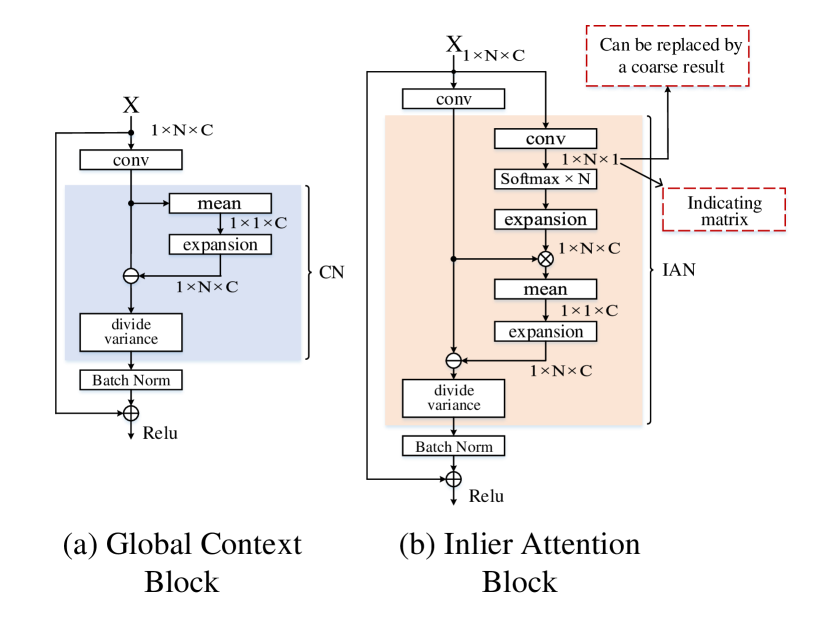
Figure 2: Comparison of Global Context Block and our IA Block.

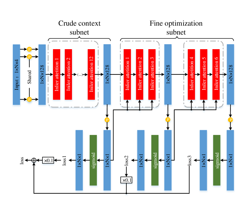
Figure 3: GLA-Net Architecture. The architecture of our GLA-Net consists of two subnet: the crude context subnet and fine optimization subnet. It is a process from coarse to fine.

Proposed Method

Problem Statement

Suppose we have a pair of images $\mathcal{(I,I^{{}^{\prime}})}$ with the coordinates of a putative correspondence set $\mathcal{(K=}$ $\{u,v\}$ $\mathcal{,K^{{}^{\prime}}=}$ $\{u^{{}^{\prime}},v^{{}^{\prime}}\}$$\mathcal{)}$ between them. The putative set is obtained by performing nearest neighbor matching on handcrafted image descriptors (e.g., SIFT) or deep learning based image descriptors (e.g. LIFT). Our method formulates the mismatch removal task as a binary classification problem and determines whether a putative match is inlier or outlier.

Guided Loss

In the classification networks, the classification of positive and negative classes is treated as a single task. They usually utilize a cost sensitive loss to address imbalance between categories as follows:

$$loss=-\frac{1}{N}(\alpha\sum_{i=1}^{N_{pos}}\log(y_{i})+\beta\sum_{j=1}^{N_{neg}}\log(1-y_{j})),$$ (1)

where $N$ is the number of putative correspondences, and $N_{pos}$ and $N_{neg}$ are number of positive and negative instances respectively. $y_{i}$ and $y_{j}$ are the network output of instance $i$ and $j$. $\alpha$ and $\beta$ are the weight coefficients of positive and negative instances. We suggest inspecting this task from another point of view. Specifically, the classification of positives and negatives are regarded as two separate issues. Then, the loss function is reconstructed as follows:

$$loss=-(\lambda\frac{1}{N_{pos}}\sum_{i=1}^{N_{pos}} \log(y_{i})+\mu\frac{1}{N_{neg}}\sum_{j=1}^{N_{neg}}\log(1-y_{j})),$$ (2)

$$s.t.\quad\ \lambda+\mu=1,$$

where $\lambda$ and $\mu$ are also weight coefficients. The other variables have the same meaning as Eq. 1. In machine learning theory, the logarithmic loss function and the 0-1 loss function have similar properties. In order to facilitate our subsequent derivation, we first replace the logarithmic loss with 0-1 loss. Suppose that after passing through the classifier, the number of misclassified instances in the positive and negative classes is $X$ and $Y$ respectively. Then the Eq. 2 can be rewritten as:

$$loss=\lambda\frac{X}{N_{pos}}+\mu\frac{Y}{N_{neg}}.$$ (3)

Since positive and negative categories are treated as two independent tasks, X and Y are independent variables.

Meanwhile, the precision ($P$) and recall ($R$) of the network can be calculated by $X$ and $Y$, and Fn-score ($Fn$) can be calculated by precision and recall. We present the relationships between these variables as follows:

$$Fn=\dfrac{(1+n^{2})\cdot P\cdot R}{n^{2}\cdot P+R},$$ (4)

$$P=\dfrac{N_{pos}-X}{N_{pos}-X+Y},R=\dfrac{N_{pos}-X}{N_{pos}}.$$ (5)

Our motivation is to establish a direct connection between loss and Fn-score. Specifically, we hope that the decrease of the loss during training will definitely lead to an increase in Fn-score. From a mathematical point of view, that means Fn-score and loss are perfectly negatively correlated. This relationship can be expressed in the form of differential as follows:

$$dloss\cdot dFn\leq 0.$$ (6)

For the convenience of derivation, we sign $\dfrac{\partial loss}{\partial X}$ as $\partial l_{X}$ and $\dfrac{\partial Fn}{\partial X}$ as $\partial F_{X}$. $Y$-related expressions are treated the same way as $X$. Then:

$$dloss=\partial l_{X}dX+\partial l_{Y}dY,dFn=\partial F_{X}dX+\partial F_{Y}dY.$$ (7)

As long as Eq. 6 is true, the decline of loss will certainly lead to the rise of Fn-score. So we start our Guided Loss from Eq. 6. We substitute Eq. 7 into Eq. 6, then:

$$\partial l_{X}\cdot\partial F_{X}\cdot(dX)^{2}+\partial l_{Y}\cdot\partial F_{Y}\cdot(dY)^{2}+$$ (8)

$$(\partial l_{X}\cdot\partial F_{Y}+\partial l_{Y}\cdot\partial F_{X})\cdot dX\cdot dY\leq 0.$$

Since $X\geq 0,Y\geq 0$ during training, We can derive the following inequality from Eq. 3, Eq. 4 and Eq. 5.

$$\partial l_{X}\geq 0,\partial l_{Y}\geq 0,\partial F_{X}\leq 0,\partial F_{Y}\leq 0.$$ (9)

In order to express Eq. 8 more clearly, we transform it into the following form:

$$(\sqrt{-\partial l_{X}\cdot\partial F_{X}}\cdot dX+\sqrt{-\partial l_{Y}\cdot\partial F_{Y}}\cdot dY)^{2}+$$ (10)

$$(\sqrt{-\partial l_{X}\cdot\partial F_{Y}}-\sqrt{-\partial l_{Y}\cdot\partial F_{X}})^{2}\cdot dX\cdot dY\geq 0.$$

In order for Eq. 10 to be the permanent establishment, then

$$\sqrt{-\partial l_{X}\cdot\partial F_{Y}}-\sqrt{-\partial l_{Y}\cdot\partial F_{X}}=0,$$ (11)

which is:

$$\dfrac{\partial F_{X}}{\partial F_{Y}}=\dfrac{\partial l_{X}}{\partial l_{Y}}.$$ (12)

Thus, Fn-score and loss are perfectly negatively correlated as long as the constraint of Eq. 12 is satisfied during the training. Based on the above derivations, we present the specific flow of our Guided Loss algorithm as Algorithm 1. Specifically, for each image pair in current training batch, we calculate the derivatives of Fn-score with respect to $X$ and $Y$ under the current network parameters. Then we can update $\lambda$ and $\mu$ by the constraint on Eq. 12. Each iteration will update $\lambda$ and $\mu$ before calculating the loss.

Algorithm 1 Guided Loss

Input: a batch of training data; last network parameter
Output: Proportion of positive and negative loss ($\lambda,\mu$)

1:  for $i=0;iter<Batch\_size;i++$ do

2:     Calculate $P_{i}$, $R_{i}$, $Fn_{i}$ of this image pair

3:     $\delta_{X_{i}}=-1$, $\delta_{Y_{i}}=0$ $\rightarrow$ $\delta_{Fn_{i}}$ $\rightarrow$ $\dfrac{\partial Fn_{i}}{\partial X_{i}}=-\delta_{Fn_{i}}$

4:     $\delta_{Fn^{{}^{\prime}}_{i}}=\delta_{Fn_{i}}$, $\delta_{X^{{}^{\prime}}_{i}}=0$, $\rightarrow$ $\delta_{Y^{{}^{\prime}}_{i}}$ $\rightarrow$ $\dfrac{\partial Fn_{i}}{\partial Y_{i}}=\dfrac{\delta_{Fn^{{}^{\prime}}_{i}}}{\delta_{Y^{{}^{\prime}}_{i}}}$ $\rightarrow$ $\dfrac{\partial Fn_{i}}{\partial X_{i}}/\dfrac{\partial Fn_{i}}{\partial Y_{i}}=-\delta_{Y_{i}^{{}^{\prime}}}$

5:     compute $\dfrac{\partial loss_{i}}{\partial X_{i}}$ and $\dfrac{\partial loss_{i}}{\partial Y_{i}}$ according to Eq. 3 $\rightarrow$ $\dfrac{\partial loss_{i}}{\partial X_{i}}$ = $\dfrac{\lambda_{i}}{N_{pos_{i}}}$, $\dfrac{\partial loss_{i}}{\partial Y_{i}}$ = $\dfrac{\mu_{i}}{N_{neg_{i}}}$

6:     s.t. $\lambda_{i}+\mu_{i}=1$ $\rightarrow$ compute $\lambda_{i}$ and $\mu_{i}$ according to Eq. 12 and the results of step 4 and 5

7:  end for

8:  return $\lambda$, $\mu$

Inlier Attention Block

Since the input of the network for mismatch removal is the unordered feature correspondences, the feature extraction blocks are required to be permutation-equivariant. Global Context Blocks are utilized as the backbone architecture in LFGC-Net (?) and its variations (?; ?). The architecture of this block in as shown in Fig. 2 (a). It extracts global context through a Context Normalization (CN) operation. CN is a simple operation that normalizes the feature maps through subtracting their means and dividing by their variances. It is very effective for processing unordered data.

However, CN completely ignores the influence of outliers on model fitting, while the features of outliers may impair the global context. In order to mitigate the negative impact of outlier on the network, we propose a IA Block architecture as shown in Fig. 2 (b). IA block replaces CN with an Inlier Attention Normalization (IAN) operation to introduce attention mechanism. Specifically, our IAN learns a soft outlier-free matrix through global context in each IA Block. This indicating matrix provides spatial variability for each instance. In SE-Net (?), the indicating matrix is directly multiplied by the feature map to magnify salient features. We also leverage simple multiplication to introduce spatial differences.

Formally, let $o_{i}^{l}\in\mathbb{R}^{C^{l}}$ be the output of $i$-th correspondence in layer $l$, where $C^{i}$ is the channel number of layer $l$. Then CN and IAN operation can both be expressed as follows:

$$Output(o_{i}^{l})=\frac{o_{i}^{l}-\mu^{l}}{\sigma^{l}},$$ (13)

where in CN :

$$\mu^{l}=\frac{1}{N}\sum_{i=1}^{N}o_{i}^{l},\sigma^{l}=\sqrt{\frac{1}{N}\sum_{i=1}^{N}(o_{i}^{l}-\mu^{l})^{2}}.$$ (14)

IAN calculates $\sigma^{l}$ in the same way as CN, but obtains $u^{l}$ in a different way, as follows:

$$\mu^{l}=\frac{1}{N}\sum_{i=1}^{N}((soft max(r^{l})*N).*o_{i}^{l}),$$ (15)

$$r^{l}=conv (o_{i}^{l}),$$

where $r^{l}$ is the indicating matrix in each IA Block. Since CN integrates global context mainly by the operation of subtracting mean, we use the indicating matrix to participate in the calculation of the mean, instead of changing the feature map. This change preserves the feature of each correspondence and filters outlier information through a weighted mean calculation. It down-weights the impacts of outliers in the process of global context extraction. Moreover, the indicating matrix can not only be automatically learned over the network, but can also replaced directly by a preliminary classification result. The visual comparison between Global Context Block and IA Block (CN and IAN operations are highlighted) is shown in the Fig. 2.

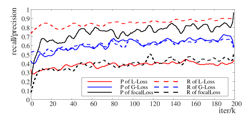
Figure 4: Precision and recall of the networks with different losses in each training iteration on the St.Brown dataset. L-Loss is the loss function that LFGC-Net (?) used. It is a cost sensitive loss with fixed weight coefficients. G-Loss is the proposed loss with F1-score’s guidance. FocalLoss (?) is a commonly used loss in object detection.

Table 1: The datasets we use to evaluate the performances of different networks. VP means viewpoint.

Dataset	# Image Pair	# Inlier Ratio(%)	Chanllenges
St.Brown	16170	7.59	Scenario changes
WIDE	11426	32.77	VP changes
COLMAP	18850	7.50	VP changes & rotation

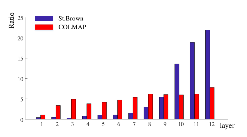
Figure 5: Attention mechanism analysis. The average ratio of weights assigned to inliers and outliers by the indicating matrix are calculated on St.Brown and COLMAP dataset to examine if the indicating matrix can assign higher weights to inliers.

GLA-Net

The whole architecture of GLA-Net is shown as Fig. 3. Inspired by the local optimization operations in geometric model-fitting methods (?; ?), the GLA-Net is developed in a coarse-to-fine manner. As shown in Fig. 3, the network can be divided into two sub-networks: crude context subnet and fine optimization subnet. Crude context subnet integrates the global context with our IA Block to get a preliminary result. During training, the preliminary result is supervised by the auxiliary loss ($loss1$ and $loss2$ in Fig. 3), which is a commonly used trick in many networks, such as GoogLeNet (?). Fine optimization subnet is designed to perform local optimization to achieve a better result. Since preliminary result has been obtained in previous subnet, IA Blocks do not learn indicating matrix, but treat the preliminary result as indicating matrix instead. The same optimization process is performed twice in this subnet.

To unite the two subnets, we combine the losses of intermediate and final results as total loss:

$$loss=\rho loss1+\eta loss2+loss3,0\leq\rho\leq 1,0\leq\eta\leq 1,$$ (16)

where $loss3$ is the main loss, and $loss1$ and $loss2$ are the auxliary losses. $\rho$ and $\eta$ are used to adjust the weights of auxliary losses.

Experiments

In this section, we first evaluate the Guided Loss and IA Block separately, and then we evaluate the overall performance with the state of the art methods. All experiments are run on Ubuntun 16.04 with NVIDIA GTX1080Ti.

Experimental Setup

Parameter Settings In our network, all the convolution kernels’ size is $(1\times 1)$. In Eq. 16, $\rho$ and $\eta$ are both set to 0.1. The auxiliary losses ($loss1$ and $loss2$) are calculated by L-Loss and the main loss ($loss3$) is by our Guided Loss, where L-Loss is the loss function used in LFGC-Net (?). Our GLA-Net is trained by Adam with a learning rate being $10^{-3}$ and batch size being 16.

Table 2: Performances of different loss functions on St.Brown and COLMAP datasets. L-Loss is the loss function that LFGC-Net (?) used. FocalLoss (?) is a commonly used loss in object detection. F1-Loss, F2-Loss and F0.5-Loss are the Guided Losses with the guidances of F1-score, F2-score and F0.5-score respectively.

Method	P(%)	R(%)	F1(%)	F2(%)	F0.5(%)
Dataset : St.Brown
L-Loss	39.72	76.83	49.83	61.35	43.08
Focal-Loss	70.67	41.44	49.67	52.77	69.11
F1-Loss	58.29	56.04	56.32	57.17	58.67
F2-Loss	47.62	66.20	54.24	62.05	51.01
F0.5-Loss	64.64	51.11	56.02	54.66	63.57
Dataset : COLMAP
L-Loss	27.95	65.63	34.83	45.67	31.03
Focal-Loss	27.52	49.44	32.32	42.03	31.78
F1-Loss	33.96	48.62	38.10	45.68	37.96
F2-Loss	32.01	49.68	37.57	48.26	37.80
F0.5-Loss	38.01	40.96	37.12	40.03	40.06

Table 3: The classification results of LFGC-Net with the same loss function but different backbones on COLMAP and WIDE datasets.

Method	P(%)	R(%)	F1(%)
Dataset : COLMAP
LFGC	33.96	48.62	38.10
LFGC with NM-Net-sp	35.42	47.12	38.25
LFGC with SE-Block	32.81	44.01	35.98
LFGC with IA-Block	37.28	62.08	43.20
Dataset : WIDE
LFGC	93.28	94.44	93.62
LFGC with NM-Net-sp	92.74	92.83	92.75
LFGC with SE-Block	93.58	93.28	93.28
LFGC with IA-Block	94.25	94.52	94.30

Table 4: Classification results of all ablation experiments on COLMAP dataset.

	P(%)	R(%)	F1(%)
Baseline	27.95	65.63	34.83
Guided Loss	33.96	48.62	38.10
IA Block	30.13	82.06	38.10
Full Framework	39.20	58.82	44.12

Benchmark Dataets All of our contrast experiments are conducted on three challenging benchmark datasets: St.Brown (?), WIDE (?) and COLMAP (?). For each dataset, their camera parameters and ground-truth labels are obtained by Structure from Motion (?). The basic properties of these three datasets are shown in Tab. 1. During training, they are divided into disjoint subsets for training (70%), validation (15%) and testing (15%).

Evaluation Criteria To measure the mismatch removal performance, we employ precision (P), recall (R), Fn-score (Fn) and average deviation between the essential matrix E estimated by selected correspondences and ground-truth $E_{gt}$ (MSE). The Fn-score can be computed as Eq. 4. In Fn, $n$ is used to adjust the importance of precision and recall in the measurement. All experimental measurements in this paper are the average values of all instances on the corresponding dataset.

Table 5: Evaluation results on COLMAP, WIDE and St.Brown datasets.

Method	P(%)	R(%)	F1(%)	MSE
Dataset : COLMAP
RANSAC	25.156	14.477	17.464	1.984
GC-RANSAC	18.785	44.239	21.226	2.976
LMR	50.776	26.070	32.482	1.962
PointNet	13.596	41.765	19.710	2.051
LFGC-Net	27.945	65.630	34.826	2.007
$\rm N^{3}$-Net	-	-	-	-
NM-Net	31.993	54.484	38.916	1.980
Ours	39.200	58.819	44.124	1.985
Dataset : WIDE
RANSAC	80.740	51.198	60.350	2.052
GC-RANSAC	68.097	88.766	76.151	2.151
LMR	84.167	78.739	82.720	2.306
PointNet	64.730	77.287	70.068	2.282
LFGC-Net	92.203	96.530	93.811	1.765
$\rm N^{3}$-Net	86.931	96.402	90.889	3.030
NM-Net	93.280	94.752	93.922	2.430
Ours	94.469	96.627	95.214	1.731
Dataset : St.Brown
RANSAC	23.743	40.831	29.322	2.659
GC-RANSAC	20.833	38.473	26.516	2.486
LMR	50.272	26.077	32.160	2.362
PointNet	27.820	47.223	32.475	3.209
LFGC-Net	39.72	76.83	49.83	3.042
$\rm N^{3}$-Net	40.923	75.341	51.683	3.023
NM-Net-sp	40.659	71.663	50.740	3.064
Ours	58.02	64.33	59.95	2.925

Submodule Performance

As discussed in method description section, our method contains two main components including Guided Loss and IA Block.

Guided Loss As shown in Tab. 2, to evaluate the performance of our Guided Loss, we train the same network architecture (In this experiments, LFGC-Net is used) with different loss functions, including L-Loss and Focal Loss. To illustrate that our Guided Loss can be employed for various measurements, we adopt different Fn-score to guide the network. In most cases, with the guidance of Fn-score, the network can achieve the best performance on this kind of measurement. This indicates that establishing a direct link between loss and measurement is conducive to improving network performance. Besides, different guiding indicators also show the stability of our guiding algorithm.

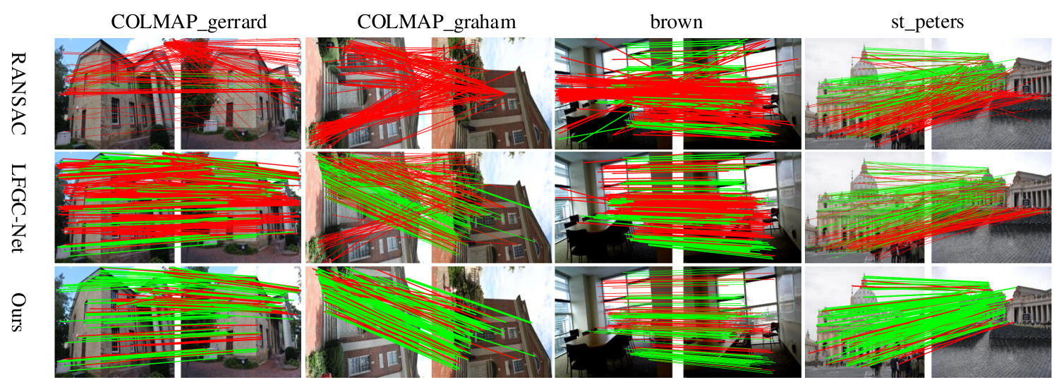
Figure 6: Visual comparison of matching results using RANSAC, LFGC-Net and our method. Images are taken from COLMAP and St.Brown datasets. Correspondences are in green if they are inliers, and in red otherwise. Best viewed in color.

Inlier Attention Block We also show the effect of our IA Block from the results of precision, recall and F1-score measurement. To directly compare the performance of the backbone block, all comparison experiments utilize the LFGC-Net network framework with our F1-score Guided Loss, and only replace the backbone of the network. As shown in Tab. 3, LFGC is the original LFGC-Net, and NM-Net-sp is the backbone of NM-Net (?) with spatial neighborhood mining. SE-Block is the attention mechanism backbone of SE-Net (?). In order to make it more suitable for mismatch removal task, we changed it to the form of spatial attention. IA Block is our proposed architecture.

As shown in Tab. 3, our architecture has achieved leadership in almost all of the three evaluation metrics (P, R, F1). Therefore, the introduction of attention mechanism can improve the performances of mismatch removal networks. In addition, the comparison with SE-Net also shows that it is better to use the indicating matrix for model fitting instead of magnifying the feature map.

Method Analysis

In order to explore the working mechanism of each module, we analyze the training process and intermediate output of the network in detail, and conduct ablation studies.

Training curve diagram We record the precision and the recall of LFGC-Net with different losses on the training set during training in Fig. 4. It can directly reflect the difference between the loss of the fixed and the variable weights. The L-Loss and focal loss all adopt a fixed weights of positive and negative classes, while G-Loss are with variable weights. The losses with fixed weights are more biased towards one measurement and ignores the other. It is difficult to assign proper weights to positive and negative classes by hand adjustment. Our G-loss can achieve a balance between precision and recall during training.

Indicating matrix In order to verify that our IA Block can be more biased to the inliers when fitting the model, we train a classification network with 12 IA blocks and record the average ratio of weights assigned to inliers and outliers. In order to confirm that the indicating matrices are automatically learned by the network, we do not use auxiliary loss trick in this experiment. As Fig. 5, the average ratio remains above 1 in most layers and increases in the later layers of the network. It shows that our IA Block is more biased towards the context of inliers, thus filtering out the influence of outliers to some extent. And the attention effect will gradually increase as the number of network layers deepens.

Ablation study We perform ablation study on the St.Brown dataset as shown in Tab. 4. The baseline network of our method is the LFGC-Net. We replace the feature extraction module and loss function in LFGC-Net with our IA Block and Guided Loss respectively. As shown in Tab. 4, the Guided Loss can achieve a balance between precision and recall, and IA Block can directly improve these two measurement. Combining these two modules can significantly improve network performance.

The Overall Performance

To test the effectiveness of our GLA-Net, we compare our GLA-Net with 7 state-of-the-art methods for mismatch removal: RANSAC (?), GC-RANSAC (?), LMR (?), pointNet (?), LFGC-Net (?), $\rm N^{3}$-Net (?), NM-Net (?). $\rm N^{3}$ cannot converge when training on the COLMAP dataset, so we do not put corresponding results on the table. NM-Net needs affine information to mine the neighborhood, while St.Brown has SIFT descriptors without affine information, so we use spatial NM-Net (nm-net-sp) instead.

As shown in Tab. 5, our method behaves favorably to both geometry and learning based methods on F1-score, especially on COLMAP and St.Brown, which are the challenging datasets with extremely low initial inlier ratios (7.50% and 7.59% respectively). For MSE measurement, all deep learning based methods obtain E matrix with similar precision.

Fig .6 shows the visual matching results of GLA-Net, our baseline (LFGC-Net) and classic RANSAC algorithm.

Conclusion

We present an end-to-end network for removing the wrong matches from the putative match set. In this network, we propose a novel Guided loss to establish the direct connection between loss and measurement, and an IA Block as feature extraction backbone to eliminate the impact of outlier on global context. We conduct extensive experiments to analyze the performance of each module and the overall network framework in detail. These experiments demonstrate that GLA-Net behaves favorably to the state-of-the-art approaches.

References

- [Akbani, Kwek, and Japkowicz 2004] Akbani, R.; Kwek, S.; and Japkowicz, N. 2004. Applying support vector machines to imbalanced datasets. In European conference on machine learning, 39–50. Springer.
- [Barath and Matas 2018] Barath, D., and Matas, J. 2018. Graph-cut ransac. In Proceedings of the IEEE Conference on Computer Vision and Pattern Recognition, 6733–6741.
- [Benhimane and Malis 2004] Benhimane, S., and Malis, E. 2004. Real-time image-based tracking of planes using efficient second-order minimization. In 2004 IEEE/RSJ International Conference on Intelligent Robots and Systems (IROS)(IEEE Cat. No. 04CH37566), volume 1, 943–948. IEEE.
- [Chawla et al. 2002] Chawla, N. V.; Bowyer, K. W.; Hall, L. O.; and Kegelmeyer, W. P. 2002. Smote: synthetic minority over-sampling technique. Journal of artificial intelligence research 16:321–357.
- [Chum and Matas 2005] Chum, O., and Matas, J. 2005. Matching with prosac-progressive sample consensus. In 2005 IEEE Computer Society Conference on Computer Vision and Pattern Recognition (CVPR’05), volume 1, 220–226. IEEE.
- [Chum, Matas, and Kittler 2003] Chum, O.; Matas, J.; and Kittler, J. 2003. Locally optimized ransac. In Joint Pattern Recognition Symposium, 236–243. Springer.
- [Dai et al. 2019] Dai, T.; Cai, J.; Zhang, Y.; Xia, S.-T.; and Zhang, L. 2019. Second-order attention network for single image super-resolution. In Proceedings of the IEEE Conference on Computer Vision and Pattern Recognition, 11065–11074.
- [Fischler and Bolles 1981] Fischler, M. A., and Bolles, R. C. 1981. Random sample consensus: a paradigm for model fitting with applications to image analysis and automated cartography. Communications of the ACM 24(6):381–395.
- [Fragoso et al. 2013] Fragoso, V.; Sen, P.; Rodriguez, S.; and Turk, M. 2013. Evsac: accelerating hypotheses generation by modeling matching scores with extreme value theory. In Proceedings of the IEEE International Conference on Computer Vision, 2472–2479.
- [He et al. 2016] He, K.; Zhang, X.; Ren, S.; and Sun, J. 2016. Deep residual learning for image recognition. In Proceedings of the IEEE conference on computer vision and pattern recognition, 770–778.
- [Hu, Shen, and Sun 2018] Hu, J.; Shen, L.; and Sun, G. 2018. Squeeze-and-excitation networks. In Proceedings of the IEEE conference on computer vision and pattern recognition, 7132–7141.
- [Lin et al. 2017] Lin, T.-Y.; Goyal, P.; Girshick, R.; He, K.; and Dollár, P. 2017. Focal loss for dense object detection. In Proceedings of the IEEE international conference on computer vision, 2980–2988.
- [Lowe 2004] Lowe, D. G. 2004. Distinctive image features from scale-invariant keypoints. International journal of computer vision 60(2):91–110.
- [Ma et al. 2019] Ma, J.; Jiang, X.; Jiang, J.; Zhao, J.; and Guo, X. 2019. Lmr: Learning a two-class classifier for mismatch removal. IEEE Transactions on Image Processing.
- [Moo Yi et al. 2018] Moo Yi, K.; Trulls, E.; Ono, Y.; Lepetit, V.; Salzmann, M.; and Fua, P. 2018. Learning to find good correspondences. In Proceedings of the IEEE Conference on Computer Vision and Pattern Recognition, 2666–2674.
- [Plötz and Roth 2018] Plötz, T., and Roth, S. 2018. Neural nearest neighbors networks. In Advances in Neural Information Processing Systems (NeurIPS).
- [Qi et al. 2017] Qi, C. R.; Su, H.; Mo, K.; and Guibas, L. J. 2017. Pointnet: Deep learning on point sets for 3d classification and segmentation. In Proceedings of the IEEE Conference on Computer Vision and Pattern Recognition, 652–660.
- [Ren et al. 2015] Ren, S.; He, K.; Girshick, R.; and Sun, J. 2015. Faster r-cnn: Towards real-time object detection with region proposal networks. In Advances in neural information processing systems, 91–99.
- [Sattler, Leibe, and Kobbelt 2009] Sattler, T.; Leibe, B.; and Kobbelt, L. 2009. Scramsac: Improving ransac’s efficiency with a spatial consistency filter. In 2009 IEEE 12th International Conference on Computer Vision, 2090–2097. IEEE.
- [Schonberger and Frahm 2016] Schonberger, J. L., and Frahm, J.-M. 2016. Structure-from-motion revisited. In Proceedings of the IEEE Conference on Computer Vision and Pattern Recognition, 4104–4113.
- [Shrivastava, Gupta, and Girshick 2016] Shrivastava, A.; Gupta, A.; and Girshick, R. 2016. Training region-based object detectors with online hard example mining. In Proceedings of the IEEE conference on computer vision and pattern recognition, 761–769.
- [Szegedy et al. 2015] Szegedy, C.; Liu, W.; Jia, Y.; Sermanet, P.; Reed, S.; Anguelov, D.; Erhan, D.; Vanhoucke, V.; and Rabinovich, A. 2015. Going deeper with convolutions. In Proceedings of the IEEE conference on computer vision and pattern recognition, 1–9.
- [Wang et al. 2018] Wang, X.; Girshick, R.; Gupta, A.; and He, K. 2018. Non-local neural networks. In Proceedings of the IEEE Conference on Computer Vision and Pattern Recognition, 7794–7803.
- [Wang et al. 2019] Wang, L.; Huang, Y.; Hou, Y.; Zhang, S.; and Shan, J. 2019. Graph attention convolution for point cloud semantic segmentation. In Proceedings of the IEEE Conference on Computer Vision and Pattern Recognition, 10296–10305.
- [Wu 2013] Wu, C. 2013. Towards linear-time incremental structure from motion. In 2013 International Conference on 3D Vision-3DV 2013, 127–134. IEEE.
- [Xiao et al. 2019] Xiao, G.; Wang, H.; Yan, Y.; and Suter, D. 2019. Superpixel-guided two-view deterministic geometric model fitting. International Journal of Computer Vision 127(4):323–339.
- [Zhao et al. 2019] Zhao, C.; Cao, Z.; Li, C.; Li, X.; and Yang, J. 2019. Nm-net: Mining reliable neighbors for robust feature correspondences. In Proceedings of the IEEE Conference on Computer Vision and Pattern Recognition, 215–224.