Gradient flow model of mode-III fracture in Maxwell-type viscoelastic materials

Abstract

We formulate a phase field crack growth model for mode III fracture in a Maxwell-type viscoelastic material. To describe viscoelastic relaxation, a field variable of viscously flowed strain is employed in addition to a displacement field and damage phase field used in the original elastic model. Unlike preceding models constructed in the mechanical engineering community, our model is based only on the generic procedure for driving (uni-directional) gradient flow system from a physically natural system energy and employ no additional assumption such as the super-imposed relations for stress and strain (and their time derivatives) valid only for linear viscoelasticity. Numerical simulations indicate that the competition between increase in deformation by applied loading and the viscoelastic relaxation determines whether a distinct crack propagation has occurred from an initial crack. Furthermore, we consider the numerical results from an energetic perspective.

1 Introduction

Fracture in soft polymeric materials is a subject closely related to modern industrial society and our daily life [1]. The endurance of tires is, for example, crucial for the safety of transportation infrastructures. In machine assembly, controlling the toughness of adhesive, i.e. weakly crosslinked polymers in rubbery state, is essential. In the food industry, comfortably and satisfyingly breaking polymers in paste or gel states is required [2].

The fracture of soft polymers involves the viscoelastic effect. Thus, its analysis is outside the applicability of the typical linear elastic fracture mechanics [3]. Thus far, several experiments have been performed regarding viscoelastic effects on the fracture of soft polymers [4, 5, 6, 7], and a variety of analytical and numerical models (primarily on the continuum scale) have been proposed to understand the experimental results [8, 9, 10, 11, 12]. With respect to the dynamical aspect, however, most theoretical models are specialised, that is, they intend to describe the fracture behaviour of specific materials in specific conditions (e.g. steady-state crack propagation in rubbers). Meanwhile, to broaden our understanding on viscoelastic fracture, a general and flexible theoretical framework that can compile the experimental and theoretical results obtained thus far is required, similar to the time-dependent Ginzburg-Landau theory for phase transition dynamics [13].

A potential candidate for such a framework is the phase field fracture model (PFFM) that was first proposed to describe quasi-brittle crack propagations in isotropic linear elastic materials [14, 15, 16] and subsequently extended to various materials with complex mechanics properties [17, 18, 19, 20] including viscoelastic materials [21, 22]. The PFFM introduces a field variable (damage phase field) representing the extent of damage (reduction in elasticity), and treats crack propagations as growth of a fully damaged narrow domain (with zero elastic modulus), instead of as the formation of a new crack surface. Hence, we can avoid the difficulty of free-boundary problems involving the motion of the crack tip that is a singular point of a stress field in typical continuum description. A key point of the currently interested PFFM is the employment of regularized system energy which coincides with the Griffith energy in the sharp crack limit [23]. By combining the regularized energy and additional assumptions on time evolution (employing gradient-flow system or almost alternative dissipative function), we can formulate fracture dynamics exhibiting high consistency with the classical Griffith theory.

For example, one of the present authors (T.T.) and Kimura formulated the dynamics of mode-III fracture in linear elastic materials by considering the gradient-flow system of a regularised system energy with respect to the deformation and the damage phase field [24, 25]. Their numerical results indicated that the derived time evolution equations (the gradient-flow system) could predict reasonable crack paths for complex boundary conditions.

This study aims to extend the gradient-flow PFFM for linear elastic materials in [24] to the mode-III fracture in a Maxwell-type viscoelastic material. An important basis of this extension is the fact that a certain class of viscoelastic constitutive relation can be described as a gradient-flow system [26]. To describe viscoelastic stress relaxation, a viscous strain is employed with the deformation field in the expression of elastic energy; a viscous strain represents the portion of the total strain flowed in a viscous manner, corresponding to a dashpot’s deformation in symbolic one-dimensional (1d) rheological models; see Fig. 1.

The gradient-flow system of the energy accords with the PDEs representing constitutive relations and the force balance condition. The two gradient-flow descriptions above (for crack propagation and for viscoelastic relaxation) are combined to formulate the dynamics of viscoelastic fracture. That is, we construct a system energy in terms of the out-of-plane displacement field, viscous strain field, and damage phase field, and derive a gradient-flow system as a set of time evolution equations of the three field quantities.

It is emphasised that our formulation does not rely on the superimposition principle for the strain rate and stress (and the resultant the convolutional stress-strain relation with the exponential kernel), which is distinctive to the linear viscoelasticity. This is the essential difference from the previous study [22]. Our formulation follows the typical mathematical procedure to derive the gradient system, that is, constructing the system energy with a clear physical meaning and deriving its gradient system to obtain a set of PDEs describing the time evolution of the system. It could, in principle, include geometrical and material nonlinearities in rheological constitutive relations, because of the independence of the superimposition principle.

Based on the obtained time evolution equations, we performed numerical simulations on a system with an initial crack subjected to mode-III (anti-plane) loading by boundary displacement with a constant velocity. The numerical result indicates that a distinct crack growth can occur from the initial crack in a quasi-brittle manner if the loading velocity is sufficiently large. Meanwhile, for a sufficiently slow loading, the system demonstrates ductility, that is, the initial notch opens progressively without extension. The crossover between ductile/(quasi-)brittle behaviours is caused by the competition between the increase in deformation by the boundary displacement and the viscoelastic relaxation. This is qualitatively consistent with experiments on some Maxwell-type viscoelastic liquids [27, 28, 29], suggesting that the present simple model (describing an artificial situation of a mode-III fracture of a Maxwell-type material) can be a prototype for more detailed modelling. Additionally, we discuss our viscoelastic PFFM from an energetic viewpoint.

2 Model

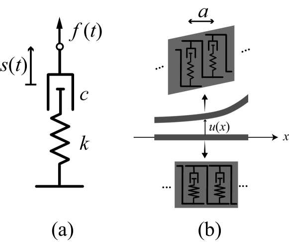
Figure 1: (a) Maxwell element with stretching deformation $s(t)$ and tension $f(t)$. (b) 1d continuum system comprising an array of innumerable vertically oriented Maxwell elements.

In this section, we explain the basic concept for describing crack propagation in viscoelastic materials as a gradient-flow system. We begin by reconsidering the mechanical behaviour of a single Maxwell element comprising a linear spring with elastic modulus $k$ and a dashpot with viscous friction constant $c$ (Fig. 1). The tension $f(t)$ acting on the element and stretching deformation $s(t)$ satisfies $f=ks_{\mathrm{e}}=c\dot{s}_{\mathrm{v}}$ and $s=s_{\mathrm{e}}+s_{\mathrm{v}}$, where $s_{\mathrm{e}}$ and $s_{\mathrm{v}}$ are the elastic deformation of the spring and the “viscously flowed” deformation of the dashpot, respectively; the dot symbol “ $\dot{\,}$ ” represents the time derivative. Eliminating $s_{\mathrm{e}}$ and $s_{\mathrm{v}}$ yields

$$\dot{f}+\left(\frac{k}{c}\right)f=c\dot{s}\,,$$ (1)

and eliminating $f$ and $s_{\mathrm{e}}$ yields

$$c\dot{s}_{\mathrm{v}}=k\left(s-s_{\mathrm{v}}\right).$$ (2)

Eq. (1) is the typical force–deformation relation of a single Maxwell element, indicating that the time derivative of force contains two contributions of the decay term with a characteristic relaxation time $\tau=c/k$ and the generation term proportional to the stretching rate $\dot{s}$. Eq. (2) indicate that the flowed component of the stretching deformation $s_{\mathrm{v}}(t)$ relaxes toward the target value $s(t)$ with the relaxation time $\tau$. It is noteworthy that $\left(s-s_{\mathrm{v}}\right)$ in the r.h.s. of eq. (2) is the elastic deformation.

Next, we discuss simple 1d continuum problem, as shown in Fig. 1(b). The system consists of innumerous identical Maxwell elements aligned along the $x$-axis with spacing $a$. The deformations of the elements are confined in the vertical direction. In the continuum description (the limit of $a\to 0$), the mechanical state of the system is described by the out-of-line displacement $u(x,t)$ and the viscous strain $e(x,t)$, i.e. the counterpart of $s_{\mathrm{v}}(t)$ of the “microscopic” Maxwell elements. The time evolution of the system is determined by the constitutive relation (corresponding with eq. (2)),

$$\eta_{\rm 1d}\dot{e}=\mu_{\rm 1d}\left(\partial_{x}u(x,t)-e\right),$$ (3)

and the motion equation,

$$\rho\ddot{u}=-\zeta_{\rm 1d}\dot{u}+\partial_{x}\mu_{\rm 1d}\left(\partial_{x}u\left(x,t\right)-e\right)\,$$ (4)

where $\mu_{\rm 1d}$ ($=ka$), $\eta_{\rm 1d}$ ($=ca$), $\rho$, and $\zeta_{\rm 1d}$ are the 1d shear modulus, 1d viscosity, 1d mass density, and 1d viscous friction coefficient for the background, respectively. When the inertia term is negligible, eqs. (3) and (4) become a set of gradient-flow equations of

$$\zeta_{\rm 1d}\dot{u}=-\frac{{\delta E}_{\rm{1d}}}{\delta u}$$ (5)

$$\eta_{\rm 1d}\dot{e}=-\frac{{\delta E}_{\rm{1d}}}{\delta e},$$ (6)

where

$$E_{\mathrm{1d}}:=\frac{\mu_{\rm 1d}}{2}\int\mathrm{d}x\left(\partial_{x}u-e\right)^{2}\$$ (7)

is the elastic (deformation) energy of this 1d model.

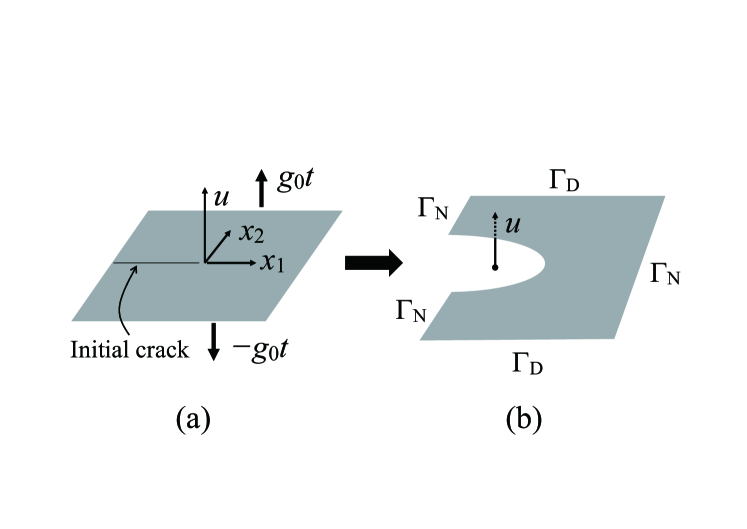
Figure 2: Computational domain in our simulation at (a) the initial state and (b) a state with an opened crack. $\Gamma_{\mathrm{D}}$ and $\Gamma_{\mathrm{N}}$ represent the Dirichlet and Neumann boundaries, respectively.

To construct a PFFM for a Maxwell-type material under mode-III loading, we consider a two-dimensional (2d) system undergoing an out-of-plane displacement $u(\mathrm{\mathbf{x}},t)$, where $\mathrm{\mathbf{x}}=(x_{1},x_{2})$ is a position vector indicating a point on the system (see Fig. 2). Furthermore, we introduce a phase field $z(\mathrm{\mathbf{x}},t)$ representing the damage of the system such that $z=0$ corresponds to a non-damaged state and $z=1$ corresponds to a completely broken state.

We assume that the total energy $E$ of the system consists of the deformation energy $E_{\mathrm{def}}$ and the damaging energy $E_{\mathrm{dam}}$:

$$E=E_{\mathrm{def}}+E_{\mathrm{dam}}\,,$$ (8)

$$E_{\mathrm{def}}:=\int_{\Omega}{\mathrm{d\mathbf{x}}\,{\left(1-z\right)^{2}\frac{\mu}{2}\left(\mathrm{\nabla}u-\mathrm{\mathbf{e}}\right)}^{2}},$$ (9)

$$E_{\mathrm{dam}}:=\frac{\gamma}{2}\int_{\mathrm{\Omega}}{\mathrm{d\mathbf{x}}\,\left(\epsilon\left|\mathrm{\nabla}z\right|^{2}+\frac{z^{2}}{\epsilon}\right)},$$ (10)

where $\Omega$ represents a 2d domain on which the model is defined, and the constants $\mu$ (N$\cdot$m^-1), $\gamma$ (N), and $\epsilon$ (m) are the 2d shear modulus, 2d fracture surface energy, and a length scale regulating the singular behaviour of the deformation field, respectively ($\epsilon$ is the thickness of a diffusive fracture surface). The integral in eq. (9) measures the length of the crack in the purely elastic model [24]. It is noteworthy that in the out-of-plane problem, the strain becomes a vector quantity $\nabla u$ (where $\nabla=(\partial/\partial x_{1},\partial/\partial x_{2})$); correspondingly, we introduce the viscous strain vector of $\mathrm{\mathbf{e}}=(e_{1},\,\,e_{2}\mathrm{)}$.

We employ the gradient-flow system of $E$ as a set of time evolution equations:

$$\alpha_{u}\dot{u}=-\frac{\delta E}{\delta u}=\mu\ \mathrm{div}\left((1-z)^{2}(\nabla u-\mathbf{e})\right)$$ (11)

$$\alpha_{e}\dot{\mathbf{e}}=-\frac{\delta E}{\delta\mathbf{e}}=\mu\,(1-z)^{2}(\nabla u-\mathbf{e})$$ (12)

$$\left(\alpha_{e}\dot{e}_{i}=-\frac{\delta E}{\delta e_{i}}=\mu\,(1-z)^{2}(\partial_{x_{i}}u-e_{i})\,\,\,\,i=1,2\,\right)$$

$$\alpha_{z}\dot{z}=\left(-\frac{\delta E}{\delta z}\right)_{+}=\left(\gamma\left(\epsilon\Delta z-\frac{z}{\epsilon}\right)+\mu\left|\nabla u-\mathbf{e}\right|^{2}(1-z)\right)_{+},$$ (13)

where the non-negative constants $\mathrm{\alpha}_{u}$, $\mathrm{\alpha}_{e}$, $\mathrm{\alpha}_{z}$ are kinetic coefficients; $\dot{A}:=\partial A/\partial t$ and the operation $(\cdot)_{+}:={\rm max}(\cdot,0)$ ensure the irreversibility of crack growth.

The following boundary conditions are imposed for $u(\mathrm{\textbf{x}},t)$ and $z(\mathrm{\textbf{x}},t)$:

$$u=g\left(\mathrm{\mathbf{x}},t\right)\,\,\,\mathrm{\mathbf{x}}\in\Gamma_{\mathrm{D}}\,,$$ (14)

$$\left(\mathrm{\nabla}u-\mathrm{\mathbf{e}}\right)\cdot\mathrm{\mathbf{n}}=0\,\,\,\mathrm{\mathbf{x}}\in\Gamma_{\mathrm{N}}\,,$$ (15)

$$\frac{\partial z}{\partial n}=0\,\,\,\,\,\mathrm{\mathbf{x}}\in\Gamma,$$ (16)

where $g\left(\mathrm{\mathbf{x}},t\right)$ is a given function, $\Gamma$ is the boundary of $\Omega$, and $\Gamma_{\mathrm{D}}$ and $\Gamma_{\mathrm{N}}$ are the parts of $\Gamma$ ($\Gamma=\Gamma_{\mathrm{D}}\cup\Gamma_{\mathrm{N}}$) with Dirichlet and Neumann boundary conditions, respectively. The time dependence of $g(\mathbf{x},t)$ implies that a protocol of boundary loading is to be prescribed. Eq. (15) represents the stress-free condition of the boundary. With adequate initial conditions of $u$ and $z$, eqs. (11)–(13) and eqs. (14)–(16) determine the time evolution of the system.

From the correspondences between eqs. (3)–(4) and eqs. (11)–(12), the constants $\alpha_{u}$ and $\alpha_{e}$ can be identified as the friction with the background and internal viscosity, respectively. We hence denote $\alpha_{\rm e}$ as $\eta$. Although $\alpha_{z}$ is of the same dimension as $\alpha_{\rm e}$ (i.e. $\eta$), its physical meaning is different: $\alpha_{z}$ can be related to the crack velocity dependence of the effective fracture energy. The details for the interpretation of $\alpha_{z}$ will be reported elsewhere. Below, we treat a special case of

$$\alpha_{u}=0$$ (17)

and

$$\alpha_{e}\gg\alpha_{z}.$$ (18)

To investigate the energy balance of the present model, we take the time derivative of the system energy, $\dot{E}=dE/dt=\int_{\Omega}dxdy\left(\frac{\delta E}{\delta u}\dot{u}+\frac{\delta E}{\delta\mathbf{e}}\dot{\mathbf{e}}+\frac{\delta E}{\delta z}\dot{z}\right)+\mathrm{B.T.}$, where B. T. means the boundary terms. With Eqs. (11)–(13), zero Neumann boundary conditions for $u$ and $z$ ((15) and (16)) and the additional conditions of (17) and (18) (that is, $\delta E/\delta u=\alpha_{u}\dot{u}=0$ and $\left(\delta E/\delta z\right)_{+}=\alpha_{z}\dot{z}\approx 0$ ), we have

$$\dot{E}=\dot{W}-\dot{Q}$$ (19)

where

$$\dot{W}=\int_{\Gamma_{\mathrm{D}}}dc\,\dot{u}\mu(1-z)^{2}(\nabla u-\mathbf{e})\cdot\mathbf{n}$$ (20)

and

$$\dot{Q}=\int_{\Omega}dxdy\,\mu(1-z)^{2}(\nabla u-\mathbf{e})\cdot\dot{\mathbf{e}}$$ (21)

are the work and heart generation per unit time of the entire system, respectively.

Eq. (19) or $\dot{W}=\dot{E}+\dot{Q}$ indicates that the work performed to the system is partitioned to system energy and heat generation.

3 Numerical results

The system is a square domain $\Omega$ with side length $L$ (i.e. $\mathbf{x}=(x_{1},x_{2})\in\Omega=(-\frac{L}{2},\frac{L}{2})^{2}$). An initial crack (highly damaged narrow zone) is prepared along the negative part of the $x_{1}$-axis (see Fig. 2). The system is loaded by anti-symmetrical displacements on $\Gamma_{\mathrm{D}}$, $u(\mathbf{x},t)|_{x_{2}=\pm L/2}=\pm g_{0}t$, where $g_{0}$ is the speed (m$\cdot$s^-1) of the boundary displacements.

For numerical simulations, we non-dimensionalise eqs. (11)–(13) by employing $L$, $T:=L/g_{0}$ and $L\mu$ as the units of length, time, and force, respectively. Introducing the non-dimensionalised quantities of $\tilde{x}_{i}=x_{i}/L$ ($\partial/\partial x_{i}=L^{-1}\partial/\partial\tilde{x}_{i}$), $\tilde{u}=u/L$, $\tilde{\varepsilon}=\varepsilon/L$, $\tilde{t}=t/T$ ($\partial/\partial t=T^{-1}\partial/\partial\tilde{t}$), $\tilde{\gamma}=\gamma/(L\mu)$, $\tilde{\alpha}_{z}=\alpha_{z}/(T\mu)$ and

$$\tilde{g}_{0}=\frac{\alpha_{e}(=\eta)}{T\mu}.$$ (22)

Eqs. (11) - (13) (with $\alpha_{u}=0$) become

$$0=\mathrm{div}\left((1-z)^{2}(\nabla u-\mathbf{e})\right)$$ (23)

$$\tilde{g}_{0}\dot{\mathbf{e}}=(1-z)^{2}(\nabla u-\mathbf{e})$$ (24)

$$\tilde{\alpha}_{z}\dot{z}=\left(\tilde{\gamma}\left(\tilde{\epsilon}\Delta z-\frac{z}{\tilde{\epsilon}}\right)+\left|\nabla u-\mathbf{e}\right|^{2}(1-z)\right)_{+},$$ (25)

where and hereinafter we omit the “ $\tilde{\ }$ ” over $u$ and $\mathbf{x}$ and $t$, and “ $\dot{\ }$ ” and $\nabla$ etc. represent the derivatives with respect to the non-dimensionalised time and spatial coordinates. (the tilde symbol for the model parameters of $\tilde{\gamma}$ $\tilde{\varepsilon}$ and $\tilde{g}_{0}$ is preserved.) Because we use $L$ as the unit of length, $\Omega=(-1/2,1/2)^{2}$ and the non-dimensionalised boundary displacement is $g_{0}t/L=t/(L/g_{0})=\tilde{t}=t$ (the last equality merely represents the omission of the tilde symbol). The boundary displacement velocity is always unity in the present non-dimensionalisation. Furthermore, the energetic quantities of $E$, $E_{\mathrm{def}}$, $E_{\mathrm{dam}}$, $W$, and $Q$ hereinafter represent the non-dimensionalised ones scaled by the characteristic energy $L^{2}\mu$. According to the these abbreviations, $\dot{E}$ represents “$(\mu L^{2}/T)^{-1}dE/dt$” in the original dimensional notation.

It is noteworthy that $\tilde{g}_{0}=\frac{g_{0}}{L/\tau}$ ($T=L/g_{0}$), where $\tau=\eta/\mu$ is the viscoelastic relaxation time; $\tilde{g}_{0}$ is the ratio between the loading velocity and the characteristic velocity of $L/\tau$.

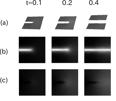
Figure 3: Temporal evolution of the three field variables of (a) deformation (bird-eye view), (b) $z$, and (c) $|\mathbf{e}|$ (gray level mapping) for $\tilde{g}_{0}=0.1$. The bright zone in (b) represents a crack.

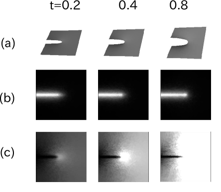
Figure 4: Temporal evolution of the three field variables of (a) deformation (bird-eye view), (b) $z$, and (c) $|\mathbf{e}|$ (gray level mapping) for $\tilde{g}_{0}=0.02$.

We set $\tilde{\gamma}=0.01$ and $\tilde{\epsilon}=0.05$, and systematically change $\tilde{g}_{0}$ from 0.02 to 10. The initial conditions are $u(\mathbf{x},0)=0$, $e_{i}(\mathbf{x},0)=0$ and $z(\mathbf{x},0)=\mathrm{exp}(-x_{2}^{\ 2}/10^{-4})/\left(1+\mathrm{exp}(x_{1}/(10^{\-2})\right)$; the third relation represents the initial crack. Actual numerical simulations were performed with FreeFem++ [30].

Figures 3 and 4 exhibit the time evolution of the field variables of the (a) displacement $u$, (b) damage phase field $z$ and (c) amplitude of the viscous strain vector $|\mathbf{e}|$ for different loading velocities of $\tilde{g}_{0}=0.1$ and 0.02.

At a relatively fast loading velocity of $\tilde{g}_{0}=0.1$, the initial crack suddenly propagates when the boundary displacement reaches a critical value. At a slow loading of $\tilde{g}_{0}=0.02$, the initial crack never extends; instead, the amplitude of the viscous strain progressively increases in the un-broken region ahead of the initial crack tip with increasing the boundary displacement, see the brightness (indicating larger $|\mathbf{e}|$) in the rightmost figure in Fig. 4(c). These two mechanical behaviour crossover at approximately $\tilde{g}_{0}=0.04$.

Figures 5(a)–(d) show $E_{\rm def}$, $E_{\rm dam}$, $\langle|\mathbf{e}|^{2}\rangle:=\int_{\Omega}dxdy|\mathbf{e}|^{2}$ and dissipation $Q(t):=\int_{0}^{t}\dot{Q}(s)ds$ (see eq. (21) for the definition of $\dot{Q}$) as functions of $t$ ($x$, $y$, and $t$ represent the non-dimensionalised quantities). Each curve in Fig. 5 shows the results for different $\tilde{g}_{0}$. For the fast deformation of $\tilde{g}_{0}=1$, $E_{\rm def}$ increases with $t$ to achieve the maximum and subsequently reduces to zero, as shown in Fig. 5(a). $E_{\rm dam}$ starts to increase at the time ($t\approx 0.1$) when $E_{\rm def}$ achieves the peak and reach its plateau at the time ($t\approx 0.18$) when $E_{\rm def}$ drops to zero (the non-zero initial value of $E_{\rm dam}$ is due to $z(\mathbf{x},0)$ giving the initial crack). . This correlated behaviour of $E_{\rm def}$ and $E_{\rm dam}$ corresponds to a distinct (quasi-brittle) crack growth Meanwhile, $\langle|\mathbf{e}|^{2}\rangle$ and $Q$ is almost zero for the fast loading (Figs. 5(c) and (d)).

For the slow deformation of $\tilde{g}_{0}=0.02$, the system exhibit ductility (see also Fig. 3) and the energetic quantities behave in the opposite manners: $E_{\rm def}$ and $E_{\rm dam}$ remain on low levels and $\langle|\mathbf{e}|^{2}\rangle$ increases progressively with $t$.

In the intermediate deformation velocity regime ($\tilde{g}_{0}=0.05$ and $0.1$), $E_{\rm def}$ achieves a peak corresponding to a distinct crack growth (and $E_{\rm dam}$ increases correlatedly with the change of $E_{\rm def}$) but the peak is dull and broaden. The dissipation $Q$ in this intermediate regime increases most rapidly until the crack growth is completed, suggesting that the crack growth involves a large amount of viscous dissipation.

To view the energy balance of the system in detail, we plot the time change of $\dot{W}$, $\dot{E}$ ($=\dot{E}_{\rm def}+\dot{E}_{\rm dam}$), and $\dot{Q}$ in Fig. 6. For the slow loading of (a) $\tilde{g}_{0}=0.02$, $\dot{E}$ remains, after the initial transient period with a small peak, low level (strictly, $\dot{E}$ slightly increases with $t$), while $\dot{W}$ and $\dot{Q}$ increase rapidly in the initial period and subsequently reach plateau regions (the plateau of $\dot{Q}$ is slightly sloped, corresponding to the slight increase in $\dot{E}_{\rm def}$). After the appearance of the plateaus,

$$\dot{W}\gtrsim\dot{Q}\gg\dot{E}$$

holds. Most of the work dissipate.

Meanwhile, for the fast loading of (c) $\tilde{g}_{0}=1$, $\dot{W}$ and $\dot{E}$ achieve shape peaks and subsequently reduce to zero, corresponding to the distinct crack growth. Before the crack growth is completed ($t\leq 0.18$), it holds that

$$\dot{W}\gtrsim\dot{E}\gg\dot{Q},$$

most of the work performed by the boundary displacement transfers into increases in the system energy, and the amount of viscous dissipation is small. The system fractures in a quasi-brittle manner.

For the intermediate loading velocity of (b) $\tilde{g}_{0}=0.1$, $\dot{W}$ and $\dot{E}$ exhibit peaks (that is, a distinct crack growth occurs), but the peaks are not shaped. Before the crack growth is completed ($t\leq 0.25$),

$$\dot{W}>\dot{Q}\approx\dot{E},$$

indicating that the system energy change is comparable to the viscous dissipation.

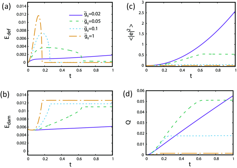
Figure 5: Temporal evolution of (a)deformation energy $E_{\textrm{def}}$, (b)damaging energy $E_{\textrm{dam}}$, (c) $\langle|\mathbf{e}|^{2}\rangle$, and (d) the total dissipation $Q$ for $\tilde{g}_{0}=0.02$ (solid line), $0.05$ (dashed line), $0.1$ (dotted line) and $1$ (long dashed dotted line).

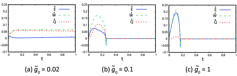
Figure 6: Temporal evolution of $\dot{E}$(solid line), $\dot{W}$(dashed line) and $\dot{Q}$(dotted line) when $\tilde{g}_{0}=0.02,0.1$ and $1.0$.

4 Discussion

As shown in Fig. 3 -6, increasing $\tilde{g}_{0}$ results in the crossover of the mechanical behaviour from ductile, for which the crack propagation is inhibited by the increase in $\mathbf{e}$, to quasi-brittle with a distinct crack propagation from the initial crack. Because $\tilde{g}_{0}=\frac{g_{0}}{L/\tau}=\frac{\tau}{T}$, distinct crack propagations occur when the viscoelastic relaxation time $\tau$ is sufficiently longer than the characteristic time of the deformation $T$. This is qualitatively consistent with experiments in Maxwell-type viscoelastic liquids [27].

The non-dimensionalised equations (23)-(25) provide a more detailed insight into the crossover in the deformation behaviour. First, it is observed that the crack extension, that is, the increase in $z$ ahead of the initial notch, is caused by the $(1-z)|\nabla u-\mathbf{e}|^{2}$ term in the r.h.s. of eq. (25).

For a very small $\tilde{g}_{0}$, Eq. (24) means $\nabla u-\mathbf{e}\approx\mathbf{0}$ for $z<1$ (the viscous strain $\mathbf{e}$ can follow $\nabla u$ without delay), thus nullifying the $(1-z)|\nabla u-\mathbf{e}|^{2}$ term. The deformation cannot drive the crack growth (ductility).

For a large $\tilde{g}_{0}$, meanwhile, $\dot{\mathbf{e}}\approx 0$ (i.e. $\mathbf{e}(\mathbf{x},t)\approx\mathbf{e}(\mathbf{x},0)=\mathbf{0}$) holds until $|\nabla u|\sim t$ exceeds $\tilde{g}_{0}$ (because $\dot{\mathbf{e}}\propto 1/\tilde{g}_{0}$, see Eq. (24)): viscoelastic relaxation barely occurs for a while from the onset of the boundary displacement. If values of $\tilde{\epsilon}$ and $\tilde{\gamma}$ allow a sudden growth of the initial crack within the elasticity dominant period ($\mathbf{e}(\mathbf{x},t)\approx\mathbf{0}$), the fracture is essentially brittle, as in the purely elastic model in [24].

In the present numerical condition, a crossover occurs at approximately $\tilde{g}_{0}=0.04$; however, the threshold value should depend on the relevant parameters of $\tilde{\gamma}$ and $\tilde{\epsilon}$, $\tilde{\alpha}_{z}(=\eta/\mu T)$.

5 Concluding remarks

In this study, we constructed a gradient flow PFFM for the mode-III fracture of a Maxwell-type viscoelastic material, by extending a purely elastic model [24]. In our formulation, utilising viscous strain is paramount. It allowed us to directly observe where and how viscoelastic relaxation occurs in the system, as in Figs. 3-5. More importantly, it provided a systematic method to recreate a model describing a particular type of elasticity (e.g. 3d linear elasticity and several hyperelasticities) into the corresponding viscoelastic PFFM. The procedure is straightforward: (i) Subtract the viscous strain from the total strain (the symmetrical part of the displacement gradient) and multiply the elastic constants by $(1-z)^{2}$ in the expression of elastic energy; (ii) Construct the total energy by adding the modified elastic energy and $E_{\rm dam}$ of Eq. (10); (iii) Derive the gradient-flow system of the total energy with respect to the deformation field, viscous strain, and damage phase field $z$. The applications of the procedure to generic 2d and 3d linear elasticities have been presented separately in [24].

Acknowledgments
We acknowledge the financial support from JSPS KAKENHI No. 17K05609. The authors thanks to Yasumasa Nishiura for his encouragement and fruitful discussions. This work is partially supported by the Cross-ministerial Strategic Innovation Promotion Program (SIP).

References

- [1] Michael F Ashby, Hugh Shercliff, and David Cebon. Materials: engineering, science, processing and design. Butterworth-Heinemann, 2018.
- [2] Ton Van Vliet. Rheology and fracture mechanics of foods. CRC Press, 2013.
- [3] Ted L Anderson. Fracture mechanics: fundamentals and applications. CRC press, 2017.
- [4] AN Gent, SM Lai, C Nah, and CHI Wang. Viscoelastic effects in cutting and tearing rubber. Rubber Chemistry and Technology, 67(4):610–618, 1994.
- [5] Wolfgang G Knauss. A review of fracture in viscoelastic materials. International Journal of Fracture, 196(1-2):99–146, 2015.
- [6] Costantino Creton and Matteo Ciccotti. Fracture and adhesion of soft materials: a review. Reports on Progress in Physics, 79(4):046601, 2016.
- [7] Xavier Poulain, Oscar Lopez-Pamies, and K Ravi-Chandar. Damage in elastomers: healing of internally nucleated cavities and micro-cracks. Soft Matter, 14(22):4633–4640, 2018.
- [8] Richard A Schapery. A theory of crack initiation and growth in viscoelastic media. International Journal of Fracture, 11(1):141–159, 1975.
- [9] Chung-Yuen Hui, Da-Ben Xu, and Edward J Kramer. A fracture model for a weak interface in a viscoelastic material (small scale yielding analysis). Journal of applied physics, 72(8):3294–3304, 1992.
- [10] PG De Gennes. Soft adhesives. Langmuir, 12(19):4497–4500, 1996.
- [11] P Rahulkumar, A Jagota, SJ Bennison, and S Saigal. Cohesive element modeling of viscoelastic fracture: application to peel testing of polymers. International Journal of Solids and Structures, 37(13):1873–1897, 2000.
- [12] BNJ Persson and EA Brener. Crack propagation in viscoelastic solids. Physical Review E, 71(3):036123, 2005.
- [13] Akira Onuki. Phase transition dynamics. Cambridge University Press, 2002.
- [14] IS Aranson, VA Kalatsky, and VM Vinokur. Continuum field description of crack propagation. Physical review letters, 85(1):118, 2000.
- [15] Blaise Bourdin, Gilles A Francfort, and Jean-Jacques Marigo. Numerical experiments in revisited brittle fracture. Journal of the Mechanics and Physics of Solids, 48(4):797–826, 2000.
- [16] Alain Karma, David A Kessler, and Herbert Levine. Phase-field model of mode iii dynamic fracture. Physical Review Letters, 87(4):045501, 2001.
- [17] Marreddy Ambati, Tymofiy Gerasimov, and Laura De Lorenzis. Phase-field modeling of ductile fracture. Computational Mechanics, 55(5):1017–1040, 2015.
- [18] Christian Miehe, M Hofacker, L-M Schänzel, and Fadi Aldakheel. Phase field modeling of fracture in multi-physics problems. part ii. coupled brittle-to-ductile failure criteria and crack propagation in thermo-elastic–plastic solids. Computer Methods in Applied Mechanics and Engineering, 294:486–522, 2015.
- [19] P Carrara and L De Lorenzis. Consistent identification of the interfacial transition zone in simulated cement microstructures. Cement and Concrete Composites, 80:224–234, 2017.
- [20] Chukwudi Chukwudozie, Blaise Bourdin, and Keita Yoshioka. A variational phase-field model for hydraulic fracturing in porous media. Computer Methods in Applied Mechanics and Engineering, 347:957–982, 2019.
- [21] Christian Miehe and Lisa-Marie Schänzel. Phase field modeling of fracture in rubbery polymers. part i: Finite elasticity coupled with brittle failure. Journal of the Mechanics and Physics of Solids, 65:93–113, 2014.
- [22] Rilin Shen, Haim Waisman, and Licheng Guo. Fracture of viscoelastic solids modeled with a modified phase field method. Computer Methods in Applied Mechanics and Engineering, 346:862–890, 2019.
- [23] L Ambrosio and VM Tortorelli. On the approximation of functionals depending on jumps by quadratic, elliptic functionals. Boll. Un. Mat. Ital, 6:105–123, 1992.
- [24] Takeshi Takaishi and Masato Kimura. Phase field model for mode iii crack growth in two dimensional elasticity. Kybernetika, 45(4):605–614, 2009.
- [25] Takeshi Takaishi. Numerical simulations of a phase field model for mode iii crack growth (theory, continuum mechanics focusing singularities, special issue joint symposium of jsiam activity groups 2009). Transactions of the Japan Society for industrial and Applied Mathematics, 19(3):351–369, 2009.
- [26] Masato Kimura, Hirofumi Notsu, Yoshimi Tanaka, and Hiroki Yamamoto. The gradient flow structure of an extended maxwell viscoelastic model and a structure-preserving finite element scheme. Journal of Scientific Computing, pages 1–21, 2019.
- [27] Joseph R Gladden and Andrew Belmonte. Motion of a viscoelastic micellar fluid around a cylinder: flow and fracture. Physical review letters, 98(22):224501, 2007.
- [28] Hervé Tabuteau, Serge Mora, Matteo Ciccotti, Chung-Yuen Hui, and Christian Ligoure. Propagation of a brittle fracture in a viscoelastic fluid. Soft Matter, 7(19):9474–9483, 2011.
- [29] Qian Huang and Ole Hassager. Polymer liquids fracture like solids. Soft Matter, 13(19):3470–3474, 2017.
- [30] Frédéric Hecht. New development in freefem++. Journal of numerical mathematics, 20(3-4):251–266, 2012.