Astronomy Reports, 2019, Vol. 63, No 11, pp. 932–943

Features of the Residual Velocity Ellipsoid of Hot Subdwarfs

from the Gaia DR2 Catalog

V.V. Bobylev and A.T. Bajkova

Central (Pulkovo) Astronomical Observatory, Russian Academy of Sciences,

Pulkovskoe shosse 65, St. Petersburg, 196140 Russia

Abstract—The evolution of the parameters of the residual velocity ellipsoid of hot subdwarfs (HSDs) with their position relative to the Galactic plane is traced, using the HSDs selected by Geier et al. from the Gaia DR2 catalog. Parameters of the Galactic rotation are determined for two $|z|$ zones. These are used to estimate the gradient of the circular rotation velocity, $V_{0},$ versus $|z|,$ found to be $\Delta V_{0}/\Delta|z|=-71\pm 7$ km s^-1 kpc^-1. The size of the residual velocity ellipsoid is $(\sigma_{1},\sigma_{2},\sigma_{3})=(36.1,27.6,22.8)\pm(0.4,0.8,0.6)$ km/s for HSDs at $|z|<0.5$ kpc and $(\sigma_{1},\sigma_{2},\sigma_{3})=(56.9,55.8,39.7)\pm(0.9,1.1,0.8)$ km/s for HSDs at $|z|\geq 0.5$ kpc. When forming the HSD residual velocities, the Galactic rotation was taken into account using individual approaches for each $z$ zone. Parameters of the residual velocity ellipsoids for HSDs located in four plane-parallel layers are also determined. The size of the ellipsoid increases with $z,$ and the inclination of the first axis relative to the Galactic plane also increases. This inclination is close to zero in zones close to the Galactic plane, $z\sim\pm 0.2$ kpc, and rises to $\mp 12\pm 4^{\circ}$ for $z\sim\pm 0.9$ kpc.

DOI: 10.1134/S1063772919110027

1 INTRODUCTION

In the Hertzsprung–Russell (HR) diagram, hot subdwarfs (sdO, sdB, sdOB) occupy a compact region at the blue end of the horizontal branch; thus, they are at late stages in the evolution of fairly massive stars. Hot subdwarfs (HSDs) are characterized by core helium burning. Such stars were first identified by Humason and Zwicky [1] in a study of super-high luminosity blue stars located near the Galactic North pole. Subsequent spectroscopy revealed hydrogen deficiencies for many HSDs. Measurements of their temperatures and surface gravities [2] made it possible to correctly identify the position of such stars in the HR diagram.

The releases of high-accuracy data from the Gaia space experiment [3, 4] opened possibilities for large-scale statistical analyses for different Galactic subsystems. The catalog contains trigonometric parallaxes and proper motions for about 1.3 billion stars. The mean uncertainties in the parallaxes of bright stars $(G<15^{m})$ are 0.02–0.04 milliarcseconds (mas), while those for faint stars $(G=20^{m})$ can be up to 0.7 mas. Similarly, the proper-motion uncertainties range from 0.05 mas/year for bright stars $(G<15^{m})$ to 1.2 mas/year for faint stars $(G=20^{m})$ [5].

Iorio and Belokurov [6] used $\sim$230 000 RR Lyrae stars from the Gaia DR2 catalog to refine the shape of the Milky Way’s halo. Rowell and Kilic [7] analyzed $\sim$79 000 white dwarfs from the Gaia DR2 catalog, obtained a new estimate of the Sun’s peculiar velocity relative to the Local Standard of Rest, and detected considerable oscillations of the vertex (the direction of the first axis of the residual velocity ellipsoid in the $xy$ plane). Vertical oscillations in the Galactic disk were analyzed using Gaia DR2 main-sequence stars [8, 9]. Using globular clusters with proper motions calculated from Gaia DR2 catalog data [10, 11], a new estimate of the Galactic mass was obtained in [12]. A considerable number of studies have dealt with refining the kinematic parameters of the thin disk [13–15], spiral structure [16, 17], and open clusters [18, 19] using data on young stars from the Gaia DR2 catalog.

The statistical and kinematic characteristics of HSDs are of considerable interest: compared to other subsystems of the Galaxy, they are not numerous and their properties remain poorly studied. An analysis of comparatively small samples demonstrates that some have properties corresponding to those of the thin disk, while others display properties of the thick disk and halo [20–22], resembling the kinematics of white dwarfs [23]. Methods aimed at searching for such stars and identifying them in large-scale surveys were developed [24], and;the first large catalogs of HSDs containing necessary data (proper motions, parallaxes) for tens of thousands of HSDs have appeared [25].

Bobylev and Bajkova [26] demonstrated that these stars display different kinematics at different positions on the celestial sphere. They considered two samples with different Galactic latitudes: low-latitude and high-latitude, dictated by the need to find scale heights. The aim of the present paper is to continue the study [26], with stars divided into zones according to their $z$ coordinates, determine parameters of the Galactic rotation in these zones, and perform a detailed study of the parameters of the velocity ellipsoid of the samples obtained.

2 METHODS

2.1 Galactic Rotation Parameters

We consider here only stars having measured proper motions. Thus, two velocities are known from observations: $V_{l}=4.74r\mu_{l}\cos b$ and $V_{b}=4.74r\mu_{b},$ directed along Galactic longitude $l$ and latitude $b$ and expressed in km/s. The coefficient 4.74 is the ratio between the number of kilometers in an astronomical unit and the number of seconds in a tropical year; $r=1/\pi$ is the star’s distance, calculated from its parallax, $\pi.$ The components of the proper motion, $\mu_{l}\cos b$ and $\mu_{b}$ are expressed in mas/year.

We determined the parameters of the Galactic rotation curve using equations derived from the formulas of Bottlinger, where we expanded the angular velocity $\Omega$ into a series, keeping terms to second power in $r/R_{0}:$

$$\begin{array}[]{lll}V_{l}=U_{\odot}\sin l-V_{\odot}\cos l+r\Omega_{0}\cos b\\ -(R-R_{0})(R_{0}\cos l-r\cos b)\Omega^{\prime}_{0}-0.5(R-R_{0})^{2}(R_{0}\cos l-r\cos b)\Omega^{\prime\prime}_{0},\end{array}$$ (1)

$$\begin{array}[]{lll}V_{b}=U_{\odot}\cos l\sin b+V_{\odot}\sin l\sin b-W_{\odot}\cos b\\ +R_{0}(R-R_{0})\sin l\sin b\Omega^{\prime}_{0}+0.5R_{0}(R-R_{0})^{2}\sin l\sin b\Omega^{\prime\prime}_{0},\end{array}$$ (2)

where $R$ is the distance between the star and the Galactic rotation axis (the corresponding cylindrical radius vector):

$$R^{2}=r^{2}\cos^{2}b-2R_{0}r\cos b\cos l+R^{2}_{0}.$$ (3)

$(U,V,W)_{\odot}$ is the sample’s group velocity, and reflects the peculiar motion of the Sun relative to the Local Standard of Rest (LSR), $V_{\odot}$ contains the component $V_{lag}$ reflecting the lag of the sample behind the LSR due to the asymmetric drift effect, $\Omega_{0}$ is the angular velocity of the Galactic rotation at the solar distance $R_{0},$ $\Omega^{\prime}_{0}$ and $\Omega^{\prime\prime}_{0}$ are the corresponding derivatives of the angular velocity, and the linear rotation velocity is $V_{0}=|R_{0}\Omega_{0}|$. The signs of the unknowns were chosen so that rotations from the $x$ axis to the $y$ axis, from $y$ to $z,$ and from $z$ to $x$ are positive. Thus, the angular velocity of the Galactic rotation will be negative here, in contrast to many other studies in which the Galactic rotation was taken to be positive, for convenience [27–29].

In the set of conditional equations (1)–(2), we determined the six unknowns $U_{\odot},$ $V_{\odot},$ $W_{\odot},$ $\Omega_{0},$ $\Omega^{\prime}_{0}$ and $\Omega^{\prime\prime}_{0}.$ from a least-squares solution to these equations. We applied weights $w_{l}=S_{0}/\sqrt{S_{0}^{2}+\sigma^{2}_{V_{l}}}$ and $w_{b}=S_{0}/\sqrt{S_{0}^{2}+\sigma^{2}_{V_{b}}},$ where $S_{0}$ is the “cosmic” dispersion (which we found beforehand for each sample; it is close to the unit weight uncertainty $\sigma_{0}$ obtained in the course of a preliminary solution of the equations); $\sigma_{V_{l}}$ and $\sigma_{V_{b}}$ are the dispersions of the uncertainties of the corresponding observed velocities. $S_{0}$ is comparable to the rms residual $\sigma_{0}$ (the unit-weight uncertainty) calculated when solving conditional equations of the form (1)–(2). We searched for the solution through several iterations using the $3\sigma$ criterion in order to eliminate stars with large residuals.

We should note here several studies aimed at determining the mean distance between the Sun and the Galactic center using individual estimates of this parameter performed over the last decade with independent methods. Examples include $R_{0}=8.0\pm 0.2$ kpc [30], $R_{0}=8.4\pm 0.4$ kpc [31], and $R_{0}=8.0\pm 0.15$ kpc [32]. We adopted $R_{0}=8.0\pm 0.15$ kpc in our study.

2.2 The Residual Velocity Ellipsoid

We estimated the dispersion of the stellar residual velocities using the following well-known method [33]. Let $U,V,W$ be the velocities along the coordinate axes $x,y,$ and $z.$ Let us consider the six second-order moments $a,b,c,f,e,d:$

$$\begin{array}[]{lll}a=\langle U^{2}\rangle-\langle U^{2}_{\odot}\rangle,\\ b=\langle V^{2}\rangle-\langle V^{2}_{\odot}\rangle,\\ c=\langle W^{2}\rangle-\langle W^{2}_{\odot}\rangle,\\ f=\langle VW\rangle-\langle V_{\odot}W_{\odot}\rangle,\\ e=\langle WU\rangle-\langle W_{\odot}U_{\odot}\rangle,\\ d=\langle UV\rangle-\langle U_{\odot}V_{\odot}\rangle,\end{array}$$ (4)

which are the coefficients of the equation for the surface

$$ax^{2}+by^{2}+cz^{2}+2fyz+2ezx+2dxy=1,$$ (5)

and also the components of the symmetric tensor of moments of the residual velocities:

$$\left(\matrix{a&d&e\cr d&b&f\cr e&f&c\cr}\right).$$ (6)

To determine the values in this tensor in the absence of radial-velocity data, the following three equations are used:

$$\begin{array}[]{lll}V^{2}_{l}=a\sin^{2}l+b\cos^{2}l\sin^{2}l-2d\sin l\cos l,\end{array}$$ (7)

$$\begin{array}[]{lll}V^{2}_{b}=a\sin^{2}b\cos^{2}l+b\sin^{2}b\sin^{2}l+c\cos^{2}b\\ -2f\cos b\sin b\sin l-2e\cos b\sin b\cos l+2d\sin l\cos l\sin^{2}b,\end{array}$$ (8)

$$\begin{array}[]{lll}V_{l}V_{b}=a\sin l\cos l\sin b+b\sin l\cos l\sin b\\ +f\cos l\cos b-e\sin l\cos b+d(\sin^{2}l\sin b-\cos^{2}\sin b),\end{array}$$ (9)

for which least-squares solutions were obtained for the six unknowns $a,b,c,f,e,d$. We then found the eigenvalues of the tensor (6): $\lambda_{1,2,3}$ by solving the secular equation:

$$\left|\matrix{a-\lambda&d&e\cr d&b-\lambda&f\cr e&f&c-\lambda\cr}\right|=0.$$ (10)

This equation’s eigenvalues are inverse squares of the semi-axes of the ellipsoid of the velocity moments; at the same time, they are the squares of the semi-axes of the residual velocity ellipsoid:

$$\begin{array}[]{lll}\lambda_{1}=\sigma^{2}_{1},\lambda_{2}=\sigma^{2}_{2},\lambda_{3}=\sigma^{2}_{3},\qquad\lambda_{1}>\lambda_{2}>\lambda_{3}.\end{array}$$ (11)

We found the directions of the main axes of the tensor (10), $L_{1,2,3}$ and $B_{1,2,3},$ from the relations:

$$\tan L_{1,2,3}={{ef-(c-\lambda)d}\over{(b-\lambda)(c-\lambda)-f^{2}}},$$ (12)

$$\tan B_{1,2,3}={{(b-\lambda)e-df}\over{f^{2}-(b-\lambda)(c-\lambda)}}\cos L_{1,2,3}.$$ (13)

We estimated the uncertainties in $L_{1,2,3}$ and $B_{1,2,3}$ using the scheme:

$$\begin{array}[]{lll}\displaystyle\varepsilon(L_{2})=\varepsilon(L_{3})={{\varepsilon(\overline{UV})}\over{a-b}},\\ \displaystyle\varepsilon(B_{2})=\varepsilon(\varphi)={{\varepsilon(\overline{UW})}\over{a-c}},\\ \displaystyle\varepsilon(B_{3})=\varepsilon(\psi)={{\varepsilon(\overline{VW})}\over{b-c}},\\ \displaystyle\varepsilon^{2}(L_{1})={\varphi^{2}\varepsilon^{2}(\psi)+\psi^{2}\varepsilon^{2}(\varphi)\over{(\varphi^{2}+\psi^{2})^{2}}},\\ \displaystyle\varepsilon^{2}(B_{1})={\sin^{2}L_{1}\varepsilon^{2}(\psi)+\cos^{2}L_{1}\varepsilon^{2}(L_{1})\over{(\sin^{2}L_{1}+\psi^{2})^{2}}},\end{array}$$ (14)

where

$$\varphi=\cot B_{1}\cos L_{1},\quad\psi=\cot B_{1}\sin L_{1}.$$

Three parameters should be computed beforehand: $\overline{U^{2}V^{2}}$, $\overline{U^{2}W^{2}}$ and $\overline{V^{2}W^{2}},$; then,

$$\begin{array}[]{lll}\displaystyle\varepsilon^{2}(\overline{UV})=(\overline{U^{2}V^{2}}-d^{2})/n,\\ \displaystyle\varepsilon^{2}(\overline{UW})=(\overline{U^{2}W^{2}}-e^{2})/n,\\ \displaystyle\varepsilon^{2}(\overline{VW})=(\overline{V^{2}W^{2}}-f^{2})/n,\end{array}$$ (15)

where $n$ is the number of stars. This method is interesting because it enables estimation of the uncertainties independently for each axis. An exception is the directions $L_{2}$ and $L_{3},$ whose uncertainties are the same because they are calculated using the same formula.

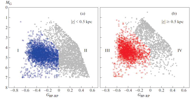
Figure 1: HR diagram for candidate HSDs with relative parallax uncertainties belower 15%. See the text for details.

DATA

We used the catalog by Geier et al. [25] for our study. This catalog contains 39 800 candidate HSDs selected from the Gaia DR2 catalog [4, 5], along with satellite and ground-based multiband photometric and spectroscopic sky surveys, including GALEX, APASS, SDSS, VISTA, 2MASS, UKIDSS,WISE, etc.

It is supposed that most candidates are HSDs of spectral types O and B, late-type B stars on the blue horizontal branch, hot stars on the asymptotic giant branch (post-AGB stars), and central stars of planetary nebulae. The authors of the catalog believe that the contamination with cooler stars is about 10%. The selected HSDs are distributed over almost the entire celestial sphere. Geier et al. [25] estimate that, with the exception of the narrow band near the Galactic plane and the zones containing the Magellanic Clouds, the catalog is complete out to a distance of 1.5 kpc. The catalog provides the parallax $\pi$ and two components of the proper motion, $\mu_{\alpha}\cos\delta$ and $\mu_{\delta},$ for each star. Radial velocities are not available. Extensive photometric information is also provided.

In our study, a zero-point correction $\Delta\pi$ was added to the Gaia DR2 parallaxes, so that the new parallax becomes $\pi+0.050$ mas. The need to take into account this systematic correction $\Delta\pi=-0.029$ mas (where the minus sign means that the correction should be added to the Gaia DR2 stellar parallaxes in order to reduce them to reference values) was first noted by Lindegren et al. [5] and confirmed by Arenou et al. [34]. Slightly later, it was demonstrated in [35–39] based on an analysis of various high-accuracy sources of distance scales that the correction was about $\Delta\pi=-0.050$ mas, with an uncertainty of several units in the last digit.

Note that the mean shift of the parallax zero point specifically for the HSDs is a matter of discussion. Some data indicate that the correction may be less significant, from about $-0.020$ to about $-0.030$ mas. This may follow, for example, from the color dependence of this systematic effect [39, 40].

We considered several sub-samples of HSD candidates. First, Geier et al. [25] noted that some 10% of the selected candidates could represent be noise. Thus, it would be interesting to understand how the kinematic parameters of the HSDs vary with position in the HR diagram. Second, a dependence of the kinematic parameters of the HSD candidates on Galactic latitude was detected in [26]. It would be more correct to look for a dependence of these parameters on distance from the Galactic $z.$ Accordingly, we compiled several HSD samples at different distances from the Galactic plane. Finally, the quality of the derived kinematic parameters depends strongly on the relative uncertainties of the parallaxes of the sample stars, $\sigma_{\pi}/\pi$. For this reason, we consider here samples with different uncertainties, $\sigma_{\pi}/\pi=30\%$ and $15\%.$

Figure 1 shows the HR diagram for the sample of HSDs. The absolute magnitudes $M_{G}$ and color indices $G_{BP-RP}$ ($Gaia_{BP-RP}$) were taken from [25]. All candidate HSDs with relative parallax uncertainties below 15% are plotted. We divided this sample into four sections, labeled using Roman numbers. Figure 1a shows stars with $|z|<0.5$ kpc and Fig. 1b those with $|z|\geq 0.5$ kpc. In addition, the stars in each panel are divided into two groups with approximately the same number of stars, according to their positions in the diagram. These two groups were identified as follows. For color indices $G_{BP-RP}<0^{m}$, the boundary line between the groups is given by $M_{G}=\tan(80^{\circ})*G_{BP-RP}+4^{m}.2$. The second boundary is the vertical line at $G_{BP-RP}=0^{m}.$ We selected the two boundary lines empirically, aiming to have approximately the same number of stars in both samples without disrupting the general character of the initial distribution.

Table 1: Parameters of the Galactic rotation derived from stars with relative parallax uncertainties below 15%

Parameters	All stars	$|z|<0.5$ kpc	$|z|\geq 0.5$ kpc
$N_{\star}$	7766	4680	3086
${\overline{r}},$ kpc	1.32	1.07	1.72
$|{\overline{z}}|,$ kpc	$0.50$	$0.24$	$0.81$
$U_{\odot},$ km/s	$11.80\pm 0.55$	$9.42\pm 0.56$	$14.4\pm 1.1$
$V_{\odot},$ km/s	$35.00\pm 0.80$	$25.44\pm 0.84$	$52.6\pm 1.6$
$W_{\odot},$ km/s	$6.02\pm 0.50$	$7.31\pm 0.45$	$4.2\pm 1.2$
$\Omega_{0},$ km s-1 kpc-1	$-26.78\pm 0.50$	$-28.68\pm 0.58$	$-23.89\pm 0.90$
$\Omega^{{}^{\prime}}_{0},$ km s-1 kpc-2	$2.67\pm 0.12$	$3.30\pm 0.14$	$2.45\pm 0.22$
$\Omega^{{}^{\prime\prime}}_{0},$ km s-1 kpc-3	$0.43\pm 0.16$	$-0.07\pm 0.20$	$0.19\pm 0.28$
$\sigma_{0},$ km/s	38.2	29.2	52.0
$A$ km s-1 kpc-1	$10.67\pm 0.49$	$13.20\pm 0.57$	$9.80\pm 0.90$
$B$ km s-1 kpc-1	$-16.11\pm 0.70$	$-15.48\pm 0.81$	$-14.09\pm 1.27$
$V_{0}$ km/s	$214\pm 6$	$229\pm 6$	$191\pm 8$
$\sigma_{1},$ km/s	$44.81\pm 0.70$	$36.74\pm 0.53$	$55.22\pm 1.29$
$\sigma_{2},$ km/s	$39.20\pm 1.10$	$27.23\pm 0.82$	$50.39\pm 1.82$
$\sigma_{3},$ km/s	$27.54\pm 0.66$	$22.40\pm 0.74$	$36.00\pm 0.98$
$L_{1},B_{1}$	$~{}11\pm 1^{\circ},$ $~{}~{}~{}~{}0\pm 1^{\circ}$	$~{}~{}7\pm 9^{\circ},$ $~{}2\pm 3^{\circ}$	$~{}14\pm 6^{\circ},~{}$ $~{}-2\pm 1^{\circ}$
$L_{2},B_{2}$	$101\pm 6^{\circ},$ $-10\pm 2^{\circ}$	$~{}97\pm 3^{\circ},$ $~{}5\pm 2^{\circ}$	$104\pm 12^{\circ},$ $-10\pm 2^{\circ}$
$L_{3},B_{3}$	$100\pm 6^{\circ},$ $~{}~{}80\pm 3^{\circ}$	$254\pm 3^{\circ},$ $84\pm 4^{\circ}$	$~{}93\pm 12^{\circ},$ $~{}~{}80\pm 4^{\circ}$

$N_{\star}$ is the number of stars used, ${\overline{r}}$ the mean distance of the stellar sample, and $\sigma_{0}$ the unit-weight uncertainty. The lower part of the table presents the main axes and orientations of the main axes for the residual velocity ellipsoids of the corresponding samples.

Table 2: Parameters of the Galactic rotation derived from stars with relative parallax uncertainties below 30%

Parameters	All stars	$|z|<0.5$ kpc	$|z|\geq 0.5$ kpc
$N_{\star}$	13253	6395	6858
${\overline{r}},$ kpc	1.81	1.31	2.28
$|{\overline{z}}|,$ kpc	$0.69$	$0.35$	$1.08$
$U_{\odot},$ km/s	$12.41\pm 0.48$	$9.84\pm 0.49$	$13.18\pm 0.80$
$V_{\odot},$ km/s	$39.96\pm 0.66$	$25.81\pm 0.70$	$58.12\pm 1.15$
$W_{\odot},$ km/s	$6.05\pm 0.44$	$7.11\pm 0.39$	$5.25\pm 0.85$
$\Omega_{0},$ km s-1 kpc-1	$-24.69\pm 0.31$	$-28.40\pm 0.39$	$-21.85\pm 0.46$
$\Omega^{{}^{\prime}}_{0},$ km s-1 kpc-2	$2.53\pm 0.08$	$3.46\pm 0.09$	$2.29\pm 0.12$
$\Omega^{{}^{\prime\prime}}_{0},$ km s-1 kpc-3	$-0.04\pm 0.06$	$-0.55\pm 0.10$	$-0.29\pm 0.09$
$\sigma_{0},$ km/s	42.7	29.0	53.7
$A$ km s-1 kpc-1	$10.12\pm 0.31$	$13.83\pm 0.37$	$9.16\pm 0.46$
$B$ km s-1 kpc-1	$-14.57\pm 0.43$	$-14.57\pm 0.54$	$-12.68\pm 0.65$
$V_{0}$ km/s	$198\pm 5$	$227\pm 5$	$175\pm 5$
$\sigma_{1},$ km/s	$47.30\pm 0.57$	$36.08\pm 0.44$	$56.91\pm 0.86$
$\sigma_{2},$ km/s	$45.65\pm 0.84$	$27.55\pm 0.76$	$55.76\pm 1.12$
$\sigma_{3},$ km/s	$31.29\pm 0.57$	$22.83\pm 0.59$	$39.67\pm 0.76$
$L_{1},B_{1}$	$~{}41\pm 6^{\circ},~{}$ $-4\pm 1^{\circ}$	$~{}10\pm 7^{\circ},$ $~{}2\pm 2^{\circ}$	$~{}37\pm 8^{\circ},~{}$ $-4\pm 1^{\circ}$
$L_{2},B_{2}$	$131\pm 14^{\circ},$ $-6\pm 1^{\circ}$	$100\pm 2^{\circ},$ $~{}5\pm 2^{\circ}$	$128\pm 19^{\circ},$ $-3\pm 2^{\circ}$
$L_{3},B_{3}$	$~{}96\pm 14^{\circ},$ $~{}83\pm 2^{\circ}$	$254\pm 2^{\circ},$ $85\pm 3^{\circ}$	$~{}73\pm 19^{\circ},$ $~{}85\pm 2^{\circ}$

The notation in the Table is the same as in Table 1.

Table 3: Parameters of the Galactic rotation derived taking into account the Lutz–Kelker bias

Parameters	$\sigma_{\pi}/\pi<15\%$	$\sigma_{\pi}/\pi<30\%$
$N_{\star}$	7656	14415
${\overline{r}},$ kpc	1.29	1.55
$U_{\odot},$ km/s	$11.56\pm 0.53$	$10.66\pm 0.40$
$V_{\odot},$ km/s	$34.50\pm 0.80$	$33.52\pm 0.55$
$W_{\odot},$ km/s	$5.90\pm 0.48$	$5.36\pm 0.37$
$\Omega_{0},$ km s-1 kpc-1	$-26.82\pm 0.50$	$-24.87\pm 0.31$
$\Omega^{{}^{\prime}}_{0},$ km s-1 kpc-2	$2.69\pm 0.12$	$2.44\pm 0.07$
$\Omega^{{}^{\prime\prime}}_{0},$ km s-1 kpc-3	$0.38\pm 0.17$	$0.38\pm 0.07$
$\sigma_{0},$ km/s	37.3	37.7
$A$ km s-1 kpc-1	$10.77\pm 0.48$	$9.74\pm 0.30$
$B$ km s-1 kpc-1	$-16.06\pm 0.68$	$-15.13\pm 0.43$
$V_{0}$ km/s	$215\pm 6$	$199\pm 5$
$\sigma_{1},$ km/s	$42.35\pm 0.59$	$42.52\pm 0.47$
$\sigma_{2},$ km/s	$36.15\pm 0.77$	$40.07\pm 0.76$
$\sigma_{3},$ km/s	$26.55\pm 0.48$	$27.73\pm 0.46$
$L_{1},B_{1}$	$~{}9\pm 1^{\circ},$   $~{}0\pm 1^{\circ}$	$~{}23\pm 4^{\circ},$  $-2\pm 1^{\circ}$
$L_{2},B_{2}$	$99\pm 4^{\circ},$  $-6\pm 1^{\circ}$	$114\pm 12^{\circ},$  $-7\pm 1^{\circ}$
$L_{3},B_{3}$	$99\pm 4^{\circ},$   $84\pm 2^{\circ}$	$~{}96\pm 12^{\circ},$  $83\pm 2^{\circ}$

The notation in the Table is the same as in Table 1.

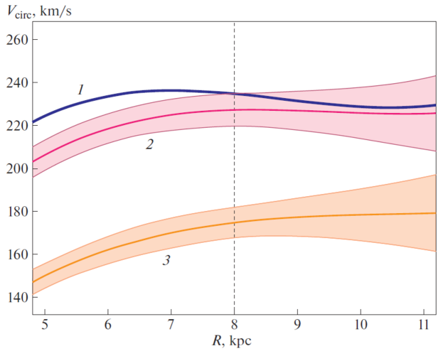
Figure 2: Galactic rotation curves plotted according to [15] (curve 1), the solution in the second-to-last column in Table 2 (curve 2), and the solution in the last column of Table 2 (curve 3). The boundaries of the confidence intervals correspond to $1\sigma.$ The vertical dashed line shows the position of the Sun.

RESULTS AND DISCUSSION

Galactic Rotation Parameters

We first divided the entire sample into groups in terms of the absolute values of their $z$ coordinates, $|z|.$ We also performed a division based on the relative uncertainty of their parallaxes. Using stars with relative parallax uncertainties below 30% provides a large number of objects and enables us to estimate the parameters of interest with lower errors. On the other hand, the sample with parallax uncertainties below 15% enables us to obtain more local parameters, in particular, more reliable estimates of the $(U,V,W)_{\odot}$ and $\Omega_{0}$.

The kinematic parameters found for these stars are collected in Tables 1 and 2. In addition to the six desired kinematic parameters, they contain the the mean distance of the sample stars ${\overline{r}},$ mean $|z|,$ unit-weight uncertainty $\sigma_{0},$ estimated from a least squares solution of the system of conditional equations of the form (1)–(2), and the Oort constants $A$ and $B,$ calculated from the relations

$$A=0.5\Omega^{{}^{\prime}}_{0}R_{0},\quad B=-\Omega_{0}+A,$$ (16)

The linear velocity of the Galactic rotation in the solar vicinity $V_{0}=|R_{0}\Omega_{0}|$ is also given. Note that we calculated the kinematic parameters presented in Tables 1 and 2 using stars with $r<6$ kpc and rejected stars with large (above 40 km/s) random errors in their measured proper motions.

The derived velocities $(U,V,W)_{\odot}$ and the Oort constants $A,B$ can be used to correct the velocities $V_{l},$ and $V_{b}$:

$$\begin{array}[]{lll}V_{l}^{*}=V_{l}-(U_{\odot}\sin l-V_{\odot}\cos l)-(A\cos 2l+B)r\cos b,\\ V_{b}^{*}=V_{b}-(U_{\odot}\cos l\sin b+V_{\odot}\sin l\sin b-W_{\odot}\cos b)+Ar\sin 2l\sin b\cos b.\end{array}$$ (17)

After this procedure, the residual velocities $V_{l}^{*}$ and $V_{b}^{*}$ should be used on the left-hand sides of (7)–(9). On the other hand, we can also form the residual velocities with the derived values of $\Omega_{0}$, $\Omega^{{}^{\prime}}_{0}$ and $\Omega^{{}^{\prime\prime}}_{0};$ note that the last term can be disregarded, since its influence in the region we are considering is negligible.

The Influence of the Lutz–Kelker Bias

Using the inverses of the parallaxes when estimating the distances results in a systematic bias of the distances obtained [27, 41–43]. The magnitude of this systematic bias depends significantly on the relative accuracy of the parallaxes and increases with the distance.

We calculated the Galactic rotation parameters and the parameters of the residual velocity ellipsoids for the two star samples taking into account the Lutz–Kelker bias. For each star with an input $\sigma_{\pi}/\pi$ value, we calculated the $G(Z)$ distribution functions using the formula modified in [27] for the case of objects with a flat space distribution:

$$G(Z)\sim Z^{-3}\exp\bigg{[}-\frac{(Z-1)^{2}}{2(\sigma_{\pi}/\pi)^{2}}\bigg{]},$$ (18)

where $Z=\pi/\pi_{true}$. The $G(Z)$ distribution function was then used to determine the factor $Z$ and the new distance, $r_{true}=1/\pi_{true}$ (the result is that the initial distances became smaller).

For this purpose, we selected HSDs with relative parallax uncertainties below 15% (the “All stars” column in Table 1) and below 30% (the “All stars” column in Table 2). The results are presented in Table 3.

These calculations demonstrated the following. For stars with relative parallax uncertainties below 15%, taking into account the influence of the Lutz–Kelker bias on the velocities of the solar motion and the Galactic rotation results in only a negligible change in the determined parameters. This influence is slightly more significant, though still small, for the dispersions of the relative velocities: $\sigma_{1},\sigma_{2},\sigma_{3}$. In general, our results agree with the conclusion of Lutz and Kelker [41] that the critical parallax error (below which there is no need to correct for the bias) is $\sigma_{\pi}/\pi:15\%-20\%$. This is also in agreement with the conclusions of [42], where it was proposed to consider a sample with parallaxes from the Gaia DR2 catalog “good” if the uncertainties for individual stars were $\sigma_{\pi}/\pi<20\%$. This led us to disregard corrections for the Lutz–Kelker bias in our analysis of stars with uncertainties $\sigma_{\pi}/\pi<15\%$.

Comparing the corresponding parameters presented in Tables 2 and 3, we can see that taking into account the Lutz–Kelker bias for stars with uncertainties $\sigma_{\pi}/\pi<30\%$ results in a more appreciable change in i the kinematic parameters. In this case, this correction has a favorable influence on the results derived from these stars. In particular, the velocity dispersions and alignment parameters of the velocity ellipsoids became closer for the two star samples presented in Table 3 after taking into account the correction.

Estimating the gradient $\Delta V_{0}/\Delta|z|$

Figure 2 shows three Galactic rotation curves. The first curve was computed by Bobylev and Bajkova [15] for a sample of stars in young open clusters. The second curve corresponds to the solution presented in the next-to-last column in Table 2, and the third curve to the solution in the last column of Table 2. The difference in the Galactic rotation velocities near the solar distance for the two derived curves is $\Delta V_{0}=52$ km/s.

We can use the data from Tables 1 and 2 to estimate the gradient of the circular rotation velocity, $V_{0},$ in $|z|.$ We found that ${\displaystyle\Delta V_{0}\over\displaystyle\Delta|z|}=-67\pm 10$ km s^-1 kpc^-1 for the sample of stars with relative parallax uncertainties $<15\%$ and ${\displaystyle\Delta V_{0}\over\displaystyle\Delta|z|}=-71\pm 7$ km s^-1 kpc^-1 for somewhat more distant and “higher” stars with relative parallax uncertainties $<30\%.$ Chiba and Beers [44] obtained the following estimates of this gradient for a sample of low metallicity stars in the solar neighborhood: ${\displaystyle\Delta V_{0}\over\displaystyle\Delta|z|}=-30\pm 3$ km s^-1 kpc^-1 for thin-disk stars with the velocity ellipsoid $(\sigma_{U},\sigma_{V},\sigma_{W})=(46,50,35)\pm(4,4,3)$ km/s; ${\displaystyle\Delta V_{0}\over\displaystyle\Delta|z|}=-52\pm 6$ km s^-1 kpc^-1 for halo stars with a very elongated velocity ellipsoid, $(\sigma_{U},\sigma_{V},\sigma_{W})=(141,106,94)\pm(11,9,8)$ km/s.

Table 4: Parameters of the residual-velocity ellipsoids for the four samples of HSDs located in four $z$ zones. Stars with relative parallax uncertainties below 15% were used

Parameters	$z<-0.5$ kpc	$-0.5\leq z<0$ kpc	$0\leq z<0.5$ kpc	$z\geq 0.5$ kpc
$N_{\star}$	1563	2494	2185	1523
${\overline{r}},$ kpc	1.71	1.07	1.06	1.75
${\overline{z}},$ kpc	$-0.91$	$-0.23$	$0.22$	$0.93$
$\sigma_{1},$ km/s	$57.1\pm 1.8$	$36.3\pm 0.9$	$36.9\pm 0.6$	$55.9\pm 1.7$
$\sigma_{2},$ km/s	$52.0\pm 2.6$	$28.5\pm 1.1$	$26.9\pm 1.2$	$49.1\pm 2.6$
$\sigma_{3},$ km/s	$30.7\pm 1.8$	$22.3\pm 1.3$	$21.6\pm 0.7$	$34.3\pm 1.3$
$L_{1},B_{1}$	$~{}~{}1^{\circ},$ $~{}~{}12\pm 4^{\circ}$	$~{}~{}7\pm 4^{\circ},$ $~{}~{}6\pm 5^{\circ}$	$~{}11\pm 2^{\circ},$ $~{}~{}0\pm 1^{\circ}$	$~{}10^{\circ},$ $-13\pm 4^{\circ}$
$L_{2},B_{2}$	$~{}89^{\circ},$ $-10\pm 4^{\circ}$	$~{}97\pm 4^{\circ},$ $~{}~{}0\pm 4^{\circ}$	$101\pm 3^{\circ},$ $10\pm 2^{\circ}$	$101^{\circ},$ $-~{}5\pm 3^{\circ}$
$L_{3},B_{3}$	$140^{\circ},$ $~{}~{}74\pm 4^{\circ}$	$188\pm 4^{\circ},$ $84\pm 5^{\circ}$	$283\pm 3^{\circ},$ $80\pm 5^{\circ}$	$~{}32^{\circ},$ $~{}~{}76\pm 5^{\circ}$

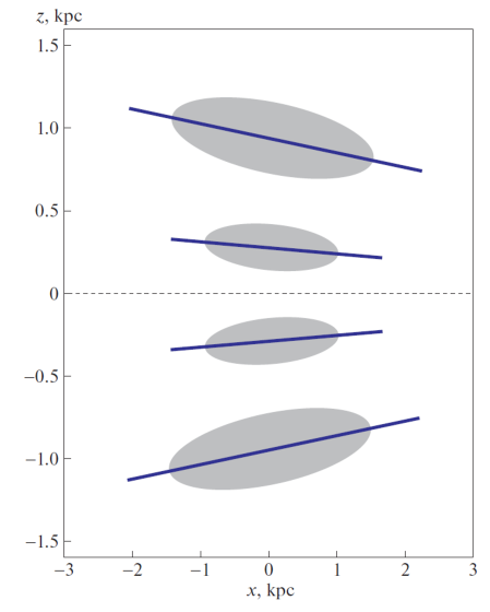
Figure 3: Schematic representation of the four derived ellipses for the $UW$ residual velocities on the $xz$ Galactic plane.

Parameters of the Velocity Ellipsoid

Table 4 presents the parameters of the residual velocity ellipsoids for the four samples of HSDs in the four z zones, two above and two below the Galactic plane. The boundaries were chosen to provide approximately the same numbers of stars in each of the samples. We took into account the dependence of the Galactic rotation on $|z|;$ i.e., we used the two rotation curves displayed in Fig. 2. The position of the first axis $L_{1},B_{1}$ deserves special attention, and is confirmed by the independently derived position of the third axis.

In the first column of Table 4, $B_{1}=12\pm 4^{\circ}$ for the most negative $z$ values, while $B_{1}=-13\pm 4^{\circ}$ for the most positive values of $z$ in the last column. The directions L1 are close, though they were determined in these zones with large uncertainties (and, for this reason, are not given in the table). Thus, we have two ellipses in the $UW$ plane, located symmetrically about the Galactic plane at heights ${\overline{z}}=\pm 0.9$ kpc; their first axes are directed towards the Galactic center at the same angles, $\mp 12^{\circ}.$ Figure 3 shows (not to scale) the projections of the four derived ellipses of the $UW$ residual velocities onto the Galactic plane $xz$.

Note also that the third axis is closer to the direction towards the pole in two regions adjacent to the Galactic plane ($|z|<0.5$ kpc), compared to regions located higher. There probably also exist effects from inhomogeneities in other planes, since some $B_{2}$ values differ significantly from zero.

Table 5: Kinematic parameters of the star samples with relative parallax uncertainties below 15%, located in two $|z|$ zones

Parameters	I	II	III	IV
	$|z|<0.5$ kpc	$|z|<0.5$ kpc	$|z|\geq 0.5$ kpc	$|z|\geq 0.5$ kpc
$N_{\star}$	2733	1947	2049	1037
${\overline{r}},$ kpc	1.08	1.04	1.55	2.05
${\overline{z}},$ kpc	$-0.91$	$-0.23$	$0.22$	$0.93$
$U_{\odot},$ km/s	$10.40\pm 0.76$	$7.64\pm 0.83$	$13.7\pm 1.1$	$11.5\pm 2.5$
$V_{\odot},$ km/s	$28.98\pm 1.25$	$20.97\pm 1.14$	$49.2\pm 1.8$	$72.7\pm 3.8$
$W_{\odot},$ km/s	$8.15\pm 0.64$	$6.12\pm 0.63$	$5.1\pm 1.3$	$4.3\pm 2.7$
$\Omega_{0},$ km s-1 kpc-1	$-28.23\pm 0.78$	$-29.44\pm 0.85$	$-24.48\pm 1.05$	$-21.2\pm 1.7$
$\Omega^{{}^{\prime}}_{0},$ km s-1 kpc-2	$3.43\pm 0.20$	$3.18\pm 0.20$	$2.86\pm 0.26$	$1.89\pm 0.41$
$\Omega^{{}^{\prime\prime}}_{0},$ km s-1 kpc-3	$-0.53\pm 0.34$	$0.37\pm 0.23$	$-1.17\pm 0.41$	$-0.23\pm 0.46$
$\sigma_{0},$ km/s	$30.8$	$26.7$	$43.9$	$65.1$
$A,$ km s-1 kpc-1	$13.73\pm 0.80$	$12.73\pm 0.80$	$11.4\pm 1.1$	$7.6\pm 1.6$
$B,$ km s-1 kpc-1	$-14.50\pm 1.11$	$-16.71\pm 1.17$	$-13.1\pm 1.5$	$-13.7\pm 2.3$
$V_{0},$ km/s	$226\pm 8$	$236\pm 8$	$196\pm 9$	$170\pm 14$
$\sigma_{1},$ km/s	$35.84\pm 0.45$	$31.02\pm 0.72$	$46.5\pm 1.2$	$67.5\pm 1.9$
$\sigma_{2},$ km/s	$26.96\pm 0.55$	$25.08\pm 0.84$	$39.6\pm 1.3$	$61.3\pm 2.1$
$\sigma_{3},$ km/s	$22.29\pm 0.41$	$19.21\pm 0.56$	$32.1\pm 0.8$	$41.8\pm 1.5$
$L_{1},B_{1}$	$~{}~{}6\pm 8^{\circ},$ $~{}~{}2\pm 4^{\circ}$	$~{}15\pm 9^{\circ},$ $~{}3\pm 3^{\circ}$	$~{}7\pm 1^{\circ},$ $~{}~{}0\pm 1^{\circ}$	$-13\pm 7^{\circ},$ $~{}~{}2\pm 1^{\circ}$
$L_{2},B_{2}$	$~{}96\pm 2^{\circ},$ $-1\pm 4^{\circ}$	$106\pm 5^{\circ},$ $~{}5\pm 2^{\circ}$	$98\pm 7^{\circ},$ $-7\pm 3^{\circ}$	$77\pm 14^{\circ},$ $-8\pm 3^{\circ}$
$L_{3},B_{3}$	$156\pm 2^{\circ},$ $87\pm 4^{\circ}$	$252\pm 5^{\circ},$ $84\pm 4^{\circ}$	$95\pm 7^{\circ},$ $83\pm 6^{\circ}$	$90\pm 14^{\circ},$ $82\pm 4^{\circ}$

The notation in the Table is the same as in Table 1.

Anguiano et al. [45] found the following dispersions from their analysis of stellar proper motions and parallaxes from the Gaia DR1 catalog [3]: $(\sigma_{U},\sigma_{V},\sigma_{W})=(33,28,23)\pm(4,2,2)$ km/s for thin-disk stars and $(\sigma_{U},\sigma_{V},\sigma_{W})=(57,38,37)\pm(6,5,4)$ km/s for thick-disk stars. They demonstrated that the deviation of the vertex in the $UV$ plane for different stellar groups varied in a very wide range, from $-5^{\circ}$ to $+40^{\circ}$, while the inclination in the $UW$ plane varied from $-10^{\circ}$ to $+15^{\circ}$ Tables 1 and 2 show that the $z$ division we used enables us to identify stars with properties close to the kinematics of the thin and thick disks.

Bobylev and Bajkova [26] found the following dispersions for a sample of low-latitude HSDs with parallax uncertainties below 15%: $(\sigma_{1},\sigma_{2},\sigma_{3})=(37.4,28.1,22.8)\pm(0.9,0.7,0.9)$ km/s. The dispersions for a high-latitude sample were $(\sigma_{1},\sigma_{2},\sigma_{3})=(51.9,46.6,34.8)\pm(1.1,1.8,0.8)$ km/s. We can see an agreement with the results of the analysis of the same stars presented in Table 1, though $\sigma_{1}$ and $\sigma_{2}$ for the high-latitude HSDs were found to be lower than the corresponding values for our subdivision into $|z|$ layers (the last column of Table 1). This difference is due primarily to the boundaries used when forming the samples.

Using data from the Gaia DR2 catalog, Hagen et al. [46] performed a large-scale study of the $(V_{R},V_{z})$ velocity plane with respect to the spatial positions of stars. They considered a region with a radius of about 4 kpc around the Sun, using stars from the Gaia DR2 catalog. Evolution of the size and alignment of the residual velocity ellipsoid with $R$ and $z$ was demonstrated. Namely, they plotted maps with a large number of ellipses whose first axes was nearly always directed towards the Galactic center (far outside the solar circle, at $R\sim 12$ kpc, the inclination becomes close to zero for any $z$). In this sense, our Fig. 3 is in agreement with the results of Hagen et al. [46], while each study derived its own sizes for the ellipses for each of the Galactic subsystems.

Examining Fig. 1, we have the impression that there are a fair number of main-sequence stars among the HSD candidates. We accordingly decided to trace changes in the kinematic parameters for the samples I–IV. Table 5 presents the kinematic parameters for four samples identified in accordance with the samples labeled with Roman numbers I–IV in Fig. 1.

We can see from Fig. 1 that the amount of contamination is small for samples I and III. This is especially true for sample III, where we see a well expressed, virtually isolated cluster of stars just in the region where HSDs should be located. The same is true for sample I; however, here, on the contrary, some of the “hundred-percent” HSDs are cut off and appear in sample II. This happened because the main clump of HSDs in Fig. 1a is more extended along the $G_{BP-RP}$ coordinate, compared to Fig. 1b. Thus, sample II also contains a large ($>60\%$) fraction of HSDs. The greatest problems in this respect occur for the sample IV, where we have many stars in the main-sequence region that are clearly separated from the main clump III. As follows from [25, Fig. 2], regions II and IV are dominated by binaries containing a cool main-sequence star as one of their components. The number of such systems is apparently fairly high in region IV.

Table 5 shows that sample II seems to be the kinematically youngest: here, the stars show the highest rotation velocity, $V_{0},$ and the lowest residual-velocity dispersions, $\sigma_{1},\sigma_{2},\sigma_{3}.$ The highest kinematic age is displayed by stars from sample IV: they have the lowest rotation velocity, $V_{0},$ and the highest residual velocity dispersions, $\sigma_{1},\sigma_{2},\sigma_{3}.$ Note that the parameters of the Galactic rotation curve derived from sample I are in good agreement with known results (and with those discussed by us above), including the second derivative of the rotation angular velocity, $\Omega^{{}^{\prime\prime}}_{0}.$

The velocity $V_{\odot}\sim 21$ km/s derived for stars in sample II demonstrates that they lag behind the LSR by only $V_{lag}=\Delta V_{\odot}\sim 8$ km/s, due to the so-called asymmetric drift. Here, we used one of the most reliable modern determinations of the Sun’s peculiar motion relative to the LSR [47]: $(U_{\odot},V_{\odot},W_{\odot})=(11.1,12.2,7.3)\pm(0.7,0.5,0.4)$ km/s. The asymmetric drift increases the $V_{lag}$ velocity for all old Galactic objects. It follows from the last column of Table 5 that the lag of the sample IV stars behind the LSR is considerable, $V_{lag}\sim 60$ km/s. On the other hand, we can see from Tables 1, 2, and 5 that there is no significant deviation from the standard value for the $U_{\odot}$ velocities; a slight difference in the $W_{\odot}$ velocity is seen for stars at high $z.$

We can use the “hundred-percent” HSDs, i.e., samples II and III, to estimate the gradient of the circular rotation velocity, $V_{0},$ in $|z|.$ This gradient is ${\displaystyle\Delta V_{0}\over\displaystyle\Delta|z|}=-52\pm 11$ km s^-1 kpc^-1 — fairly moderate, closer to the more reliable results obtained by Chiba and Beers [44] based on a large number of data points. Samples I and IV give the estimate ${\displaystyle\Delta V_{0}\over\displaystyle\Delta|z|}=-74\pm 16$ km s^-1 kpc^-1.

The parameters of the residual stellar-velocity ellipsoids presented in Table 5 agree with the parameters in Table 1. Since the sign of the velocity is averaged when considering $|z|$ layers, we do not find any serious deviations in the ellipsoid alignment with respect to the $x,y,z$ coordinate axes. Though the semi-major axes of the velocity ellipsoid found for sample IV are the largest among those derived in our study, they nevertheless fall short of corresponding values for the halo.

CONCLUSION

We have studied the kinematics of HSDs from the catalog of Geier et al. [25], selected from the Gaia DR2 catalog, in conjunction with data from several multi-band photometric sky surveys. Our study made use of more than 13 000 proper motions for stars with relative parallax uncertainties below 30%. A zero-point correction, $\Delta\pi=0.050$ mas, was added to all parallaxes from the Gaia DR2 catalog.

We used two samples of stars with relative parallax uncertainties below 15% and 30% to study the influence of the Lutz–Kelker bias [41]. The influence of this bias on the derived parameters of the Sun’s peculiar motion, Galactic rotation, and residual-velocity ellipsoid was demonstrated to be negligible for uncertainties below 15

We determined the parameters of the Galactic rotation for two $|z|$ zones. The linear rotation velocity found for the HSDs at $|z|<0.5$ kpc is $V_{0}=227\pm 5$ km/s. This indicates that these stars belong to the Galactic thin disk, as is also confirmed by the semi-major axes of their residual velocity ellipsoid: $(\sigma_{1},\sigma_{2},\sigma_{3})=(36.1,27.6,22.8)\pm(0.4,0.8,0.6)$ km/s.

The HSDs at $|z|\geq 0.5$ kpc display a considerably lower rotation velocity, $V_{0}=175\pm 5$ km/s, typical of thick-disk objects. The semi-major axes found for their residual-velocity ellipsoid also suggest membership in the thick disk: $(\sigma_{1},\sigma_{2},\sigma_{3})=(56.9,55.8,39.7)\pm(0.9,1.1,0.8)$ km/s. We used these data to estimate the gradient of the circular rotation velocity, $V_{0},$ in $|z|$ to be $\Delta V_{0}/\Delta|z|=-71\pm 7$ km s^-1 kpc^-1.

We also considered samples with the most probable HSD candidates. These give the estimate $\Delta V_{0}/\Delta|z|=-52\pm 11$ km s^-1 kpc^-1. Using such stars (sample III) at $|z|\geq 0.5$ kpc zone, we found more moderate semi-major axes for their residual velocity ellipsoid: $(\sigma_{1},\sigma_{2},\sigma_{3})=(46.5,39.6,32.1)\pm(1.2,1.3,0.8)$ km/s.

When forming the stellar residual velocities, we took into account the Galactic rotation separately for each $z$ zone. The parameters of the residual velocity ellipsoids were obtained for HSDs in four plane-parallel layers. The the size of the ellipsoid increases with $z,$ as does the inclination of the first axis to the Galactic plane.

We have shown that, at $|z|<0.5$ kpc, the possible contamination of the sample of candidate HSDs comprises only a small fraction, related to kinematically cooler, younger main-sequence stars that have little influence on the derived kinematic parameters. However, the contamination could be higher at $|z|\geq 0.5$ kpc, associated with stars with higher velocity dispersions; i.e., stars that are hotter in a kinematic sense.

ACKNOWLEDGEMENTS

The authors thank the referee for useful remarks that helped us to improve the paper.

REFERENCES

1. M.L. Humason and F. Zwicky, Astrophys. J. 105, 85 (1947).

2. J.L. Greenstein and A.I. Sargent, Astrophys. J. Suppl. 28, 157 (1974).

3. Gaia Collaboration, A.G.A. Brown, A. Vallenari, T. Prusti, J. de Bruijne, F. Mignard, R. Drimmel, et al., Astron. Astrophys. 595, 2 (2016).

4. Gaia Collaboration, A.G.A. Brown, A. Vallenari, T. Prusti, de Bruijne, C. Babusiaux, C.A.L. Bailer-Jones, M. Biermann, D.W. Evans, et al., Astron. Astrophys. 616, 1 (2018).

5. Gaia Collaboration, L. Lindegren, J. Hernandez, A. Bombrun, S. Klioner, U. Bastian, M. Ramos-Lerate, A. de Torres, H. Steidelmuller, et al., Astron. Astrophys. 616, 2 (2018).

6. G. Iorio and V. Belokurov, Mon. Not. R. Astron. Soc. 482, 3868 (2019).

7. N. Rowell and M. Kilic, Mon. Not. R. Astron. Soc. 484, 3544 (2019).

8. T. Antoja, A. Helmi, M. Romero-Gómez, D. Katz, C. Babusiaux, R. Drimmel, D. W. Evans, F. Figueras, et al., Nature 561, 360 (2018).

9. M. Bennett and J. Bovy, Mon. Not. R. Astron. Soc. 482, 1417 (2019).

10. E. Vasiliev, Mon. Not. R. Astron. Soc. 484, 2832 (2019).

11. H. Baumgardt, M. Hilker, A. Sollima, and A. Bellini, Mon. Not. R. Astron. Soc. 482, 5138 (2019).

12. G. Eadie and M. Juric, Astrophys. J. 875, 159 (2019).

13. D. Kawata, J. Bovy, N. Matsunaga, and J. Baba, Mon. Not. R. Astron. Soc. 482, 40 (2019).

14. V.V. Bobylev and A.T. Bajkova, Astron. Lett. 44, 675 (2018).

15. V.V. Bobylev and A.T. Bajkova, Astron. Lett. 45, 109 (2019).

16. J.A.S. Hunt, J. Hong, J. Bovy, D. Kawata, and R.J.J. Grand, Mon. Not. R. Astron. Soc. 481, 3794 (2018).

17. J.A. Sellwood, W.H. Trick, R.G. Carlberg, J. Coronado, and H.-W. Rix, Mon. Not. R. Astron. Soc. 484, 3154 (2019).

18. W.S. Dias, H. Monteiro, J.R.D. Lépine, R. Prates, C.D. Gneiding, and M. Sacchi, Mon. Not. R. Astron. Soc. 481, 3887 (2018).

19. C. Soubiran, T. Cantat-Gaudin, M. Romero-Gomez, L. Casamiquela, C. Jordi, A. Vallenari, T. Antoja, L. Balaguer-Núñez, et al., Astron. Astrophys. 619, 155 (2018).

20. M. Altmann, H. Edelmann, and K.S. de Boer, Astron. Astrophys. 414, 181 (2004).

21. S.K. Randall, S. Bagnulo, E. Ziegerer, S. Geier, and G. Fontaine, Astron. Astrophys. 576, 65 (2015).

22. P. Martin, C.S. Jeffery, N. Naslim, and V.M. Woolf, Mon. Not. R. Astron. Soc. 467, 68 (2017).

23. E.-M. Pauli, R. Napiwotzki, U. Heber, M. Altmann, and M. Odenkirchen, Astron. and Astrophys. 447, 173 (2006).

24. Y. Bu, Z. Lei, G. Zhao, J. Bu, and J. Pan, Astrophys. J. Suppl. Ser. 233, 2 (2017).

25. S. Geier, R. Raddi, N.P. Gentile Fusillo, and T.R. Marsh, Astron. Astrophys. 621, 38 (2019).

26. V.V. Bobylev and A.T. Bajkova, Astron. Lett. 45 (2019, in press).

27. A.S. Rastorguev, M.V. Zabolotskikh, A.K. Dambis, et al., Astrophys. Bulletin, 72, 122 (2017).

28. V.V. Vityazev, A.S. Tsvetkov, V.V. Bobylev, et al., Astrophysics, 60, 462 (2017).

29. V.V. Bobylev and A.T. Bajkova, Astron. Lett. 43, 452 (2017).

30. J.P. Vallée, Astrophysics and Space Science 362, 79 (2017).

31. R. de Grijs and G. Bono, Astrophys. J. Suppl. Ser. 232, 22 (2017).

32. T. Camarillo, M. Varun, M. Tyler, and R. Bharat), PASP 130, 4101 (2018).

33. K.F. Ogorodnikov, Dynamics of stellar systems (Oxford: Pergamon, ed. Beer, A. 1965).

34. Gaia Collaboration, F. Arenou, X. Luri, C. Babusiaux, C. Fabricius, A. Helmi, T. Muraveva, A.C. Robin, F. Spoto, et al., Astron. Astrophys. 616, 17 (2018).

35. K.G. Stassun and G. Torres, Astrophys. J. 862, 61 (2018).

36. A.G. Riess, S. Casertano, W. Yuan, L. Macri, B. Bucciarelli, M.G. Lattanzi, J.W. MacKenty, J.B. Bowers, et al., Astrophys. J. 861, 126 (2018).

37. J.C. Zinn, M.H. Pinsonneault, D. Huber, and D. Stello, arXiv: 1805.02650 (2018).

38. L.N. Yalyalieva, A.A. Chemel, E.V. Glushkova, A.K. Dambis, and A.D. Klinichev, Astrophys. Bulletin, 73, 335 (2018).

39. H.W. Leung and J. Bovy, arXiv:1902.08634 (2019).

40. D. Graczyk, G. Pietrzynski, W. Gieren, J. Storm, N. Nardetto, A. Gallenne, P. Maxted, P. Kervella, et al., Astrophys. J. 872, 85 (2019).

41. T.E. Lutz and D.H. Kelker, PASP 85, 573 (1973).

42. C.A.L. Bailer-Jones, PASP 127, 994 (2015).

43. Gaia Collaboration, X. Luri, A.G.A. Brown, L.M. Sarro, F. Arenou, C.A.L. Bailer-Jones, A. Castro-Ginard, J. de Bruijne, T. Prusti, et al., Astron. and Astrophys. 616, 9 (2018).

44. M. Chiba and T.C. Beers, Astron. J. 119, 2843 (2000).

45. B. Anguiano, S.R. Majewski, K.C. Freeman, A.W. Mitschang, and M.C. Smith, Mon. Not. R. Astron. Soc. 474, 854 (2018).

46. J.H.J. Hagen, A. Helmi, P.T. de Zeeuw, and L. Posti, arXiv:1902.05268 (2019).

47. R. Schönrich, J. Binney, and W. Dehnen, Mon. Not. R. Astron. Soc. 403, 1829 (2010).