Hidden-charm and hidden-bottom molecular pentaquarks in chiral perturbation theory

Abstract

The newly observed $P_{c}(4312)$, $P_{c}(4440)$ and $P_{c}(4457)$ at the LHCb experiment are very close to the $\Sigma_{c}\bar{D}$ and $\Sigma_{c}\bar{D}^{\ast}$ thresholds. In this work, we perform a systematic study and give a complete picture on the interactions between the $\Sigma_{c}^{(\ast)}$ and $\bar{D}^{(\ast)}$ systems in the framework of heavy hadron chiral perturbation theory, where the short-range contact interaction, long-range one-pion-exchange contribution, and intermediate-range two-pion-exchange loop diagrams are all considered. We first investigate the three $P_{c}$ states without and with considering the $\Lambda_{c}$ contribution in the loop diagrams. It is difficult to simultaneously reproduce the three $P_{c}$s unless the $\Lambda_{c}$ is included. The coupling between the $\Sigma_{c}^{(\ast)}\bar{D}^{(\ast)}$ and $\Lambda_{c}\bar{D}^{(\ast)}$ channels is crucial for the formation of these $P_{c}$s. Our calculation supports the $P_{c}(4312)$, $P_{c}(4440)$ and $P_{c}(4457)$ to be the $S$-wave hidden-charm $[\Sigma_{c}\bar{D}]_{J=1/2}^{I=1/2}$, $[\Sigma_{c}\bar{D}^{\ast}]_{J=1/2}^{I=1/2}$ and $[\Sigma_{c}\bar{D}^{\ast}]_{J=3/2}^{I=1/2}$ molecular pentaquarks, respectively. Our calculation disfavors the spin assignment $J^{P}=\frac{1}{2}^{-}$ for $P_{c}(4457)$ and $J^{P}=\frac{3}{2}^{-}$ for $P_{c}(4440)$, because the excessively enhanced spin-spin interaction is unreasonable in the present case. We obtain the complete mass spectra of the $[\Sigma_{c}^{(\ast)}\bar{D}^{(\ast)}]_{J}$ systems with the fixed low energy constants. Our result indicates the existence of the $[\Sigma_{c}^{\ast}\bar{D}^{\ast}]_{J}~{}(J=\frac{1}{2},\frac{3}{2},\frac{5}{2})$ hadronic molecules. The previously reported $P_{c}(4380)$ might be a deeper bound one. Additionally, we also study the hidden-bottom $\Sigma_{b}^{(\ast)}B^{(\ast)}$ systems, and predict seven bound molecular states, which could serve as a guidance for future experiments. Furthermore, we also examine the heavy quark symmetry breaking effect in the hidden-charm and hidden-bottom systems by taking into account the mass splittings in the propagators of the intermediate states. As expected, the heavy quark symmetry in the bottom cases is better than that in the charmed sectors. We notice that the heavy quark symmetry in the $\Sigma_{c}\bar{D}$ and $\Sigma_{c}^{\ast}\bar{D}$ systems is much worse for some fortuitous reasons. The heavy quark symmetry breaking effect is nonnegligible in predicting the effective potentials between the charmed hadrons.

1 Introduction

The charmonium physics is one of the most charming and interesting sectors in quantum chromodynamics (QCD). On the one hand, the charmonium spectra deepen our understanding on the nonperturbative QCD and serve as a good platform to develop multifarious potential models. On the other hand, the discoveries of the exotic $XYZ$ states challenge the conventional hadron spectra Chen:2016qju , since these states cannot be easily reconciled with the predictions of the conventional quark models. Furthermore, the heavy quark symmetry in the charm sector is not good enough, thus the heavy quark symmetry breaking effect would manifest itself and lead to some novel phenomena sometimes.

In 2015, two pentaquark candidates $P_{c}(4380)$ and $P_{c}(4450)$ were observed by the LHCb Collaboration in the $J/\psi p$ invariant mass spectrum via the weak decay process of $\Lambda_{b}^{0}\to J/\psi pK^{-}$ Aaij:2015tga . The discovery of these two exotica triggered many discussions on the their internal structures (for some related reviews, see refs. Chen:2016qju ; Guo:2017jvc ; Liu:2019zoy ; Lebed:2016hpi ; Esposito:2016noz ; Brambilla:2019esw ), among which, the molecular interpretation is the most favored one. In ref. Chen:2015loa , these two states are interpreted as the deeply bound $\Sigma_{c}\bar{D}^{\ast}$ and $\Sigma_{c}^{\ast}\bar{D}^{\ast}$ molecular states in the framework of one-pion-exchange model. Whereas in ref. He:2015cea , they are regarded as the $\Sigma_{c}^{\ast}\bar{D}$ and $\Sigma_{c}^{\ast}\bar{D}^{\ast}$ molecules, respectively. However, the $J^{P}$ quantum numbers of the $P_{c}(4380)$ and $P_{c}(4450)$ remain an open question.

Very recently, the LHCb Collaboration reported the new results with the updated data Aaij:2019vzc . A new narrow state $P_{c}(4312)$ is observed in the $J/\psi p$ mass spectrum. In addition, the previously observed structure $P_{c}(4450)$ is dissolved into two narrow peaks $P_{c}(4440)$ and $P_{c}(4457)$. Since these three states lie several to tens MeV below the thresholds of $\Sigma_{c}\bar{D}$ and $\Sigma_{c}\bar{D}^{\ast}$, the molecular explanation is proposed with the chiral perturbation theory Meng:2019ilv , contact-range effective field theory Liu:2019tjn , one-boson-exchange model Chen:2019asm , local hidden gauge formalism Xiao:2019aya , and Bethe-Salpeter equation approach He:2019ify , respectively. The decays and productions of the $P_{c}$ states are also studied in refs. Xiao:2019mst ; Sakai:2019qph ; Voloshin:2019aut ; Wang:2019krd (one can see refs. Guo:2019fdo ; Ali:2019npk ; Guo:2019kdc ; Weng:2019ynv ; Burns:2019iih for some other pertinent works).

The interactions between $\Sigma_{c}^{(\ast)}$ and $\bar{D}^{(\ast)}$ are essential to map out the mass spectra of the $\Sigma_{c}^{(\ast)}\bar{D}^{(\ast)}$ molecules. Before the discovery of these $P_{c}$ states, the $\Sigma_{c}^{(\ast)}\bar{D}^{(\ast)}$ interactions have been investigated with the one-boson-exchange model Wu:2010jy ; Yang:2011wz and chiral quark model Wang:2011rga . In this work, in light of the newly observed $P_{c}(4312)$, $P_{c}(4440)$ and $P_{c}(4457)$ Aaij:2019vzc , we systematically study the $\Sigma_{c}^{(\ast)}$ and $\bar{D}^{(\ast)}$ interactions with chiral perturbation theory up to the one-loop level.

Nowadays, as the one inheritor of the Yukawa theory, the one-boson-exchange model is the most popular and economical formalism for depicting the nucleon-nucleon ($N$-$N$) systems Stoks:1994wp ; Machleidt:2000ge and $XYZ$ states Chen:2016qju . But in this model, one has to include as many exchanged particles as possible, such as $\pi$, $\sigma$, $\rho$, $\omega$, or higher states and so on. As the other inheritor of the Yukawa theory, chiral perturbation theory plays a pivotal role in the modern theory of nuclear force. Its degrees of freedom are unambiguous, i.e., the pion and matter field. Another advantage of chiral perturbation theory is its consistent power counting. The scattering amplitude can be expanded order by order with a small parameter $\varepsilon$ (generally, $\varepsilon=m_{\pi}/\Lambda_{\chi}$ or $q/\Lambda_{\chi}$, where $m_{\pi}$ and $q$ are the mass and momentum of pion, respectively, and $\Lambda_{\chi}\simeq 1$ GeV is the chiral breaking scale). Therefore, the error is estimable and controllable. In the past decades, the chiral perturbation theory has been extensively exploited to study the $N$-$N$ systems with great success Bernard:1995dp ; Epelbaum:2008ga ; Machleidt:2011zz ; Meissner:2015wva ; Hammer:2019poc . Moreover, in recently years, this theory is also employed to investigate the effective potentials of the $DD^{\ast}$ Xu:2017tsr , $\bar{B}^{(*)}\bar{B}^{(*)}$ Liu:2012vd ; Wang:2018atz , and $\Sigma_{c}\bar{D}^{(*)}$ Meng:2019ilv systems.

The interactions between heavy matter fields in the chiral perturbation theory are clear and straightforward, which generally include the long-range one-pion-exchange, intermediate-range two-pion-exchange and short-range contact interaction Machleidt:2011zz ; Weinberg:1990rz ; Weinberg:1991um . The contributions from the heavy degrees of freedom are encoded into the low energy constants (LECs) of the contact Lagrangians. As we know, the masses of the heavy matter fields, like $\Sigma_{c}^{(\ast)}$ and $\bar{D}^{(\ast)}$, do not vanish in the chiral limit. The large masses would break the chiral power counting. Thus, we can adopt the heavy hadron reduction formalism to integrate out the large mass scale Georgi:1990um ; Jenkins:1990jv ; Cho:1992cf . For the loop diagrams generated by the two-pion-exchange interactions, we will encounter another trouble, which also destroys the power counting rule. Considering the one-loop Feynman diagrams illustrated in figure 1, the scattering amplitude at the leading order of the nonrelativistic expansion is badly divergent because of the pinch singularity Machleidt:2011zz ; Weinberg:1991um . Although the problem of divergence can be solved by including the kinetic energies of $\Sigma_{c}^{(*)}$ and $\bar{D}^{\ast}$ at the leading order (see some more detailed discussions in refs. Machleidt:2011zz ; Weinberg:1991um ; Wang:2018atz ), the amplitude would be finally enhanced by a large factor $M/|\bm{p}|$ ($M$ could be the mass of $\Sigma_{c}^{(*)}$ or $\bar{D}^{\ast}$), which will destroy the power counting as well. This strong enhancement is the manifestation of the nonperturbative nature of the nuclear force, which is responsible for the existence of the bound pentaquark states. In other words, a nonperturbative treatment is required.

In the two seminal works Weinberg:1990rz ; Weinberg:1991um , Weinberg pointed out that we shall focus on the effective potential, i.e, the contributions from two-particle-irreducible (2PI) graphs. The two-particle-reducible (2PR) part, that originates from the on-shell intermediate $\Sigma_{c}^{(\ast)}$ and $\bar{D}^{\ast}$, should be subtracted. On the other hand, the 2PR part can be automatically recovered when the one-pion-exchange potential is inserted into the nonperturbative iterative equation, such as the Schrödinger equation or Lippmann-Schwinger equation. Therefore, the 2PI parts in the diagrams of figure 1 that contribute to the effective potentials can still be calculated perturbatively. We just need to solve a nonperturbative iterative equation with the obtained effective potential eventually.

For the $\Sigma_{c}^{(*)}\bar{D}^{(*)}$ systems, the mass splittings in the spin doublets $(\Sigma_{c},\Sigma_{c}^{\ast})$ and $(\bar{D},\bar{D}^{\ast})$ do not vanish in the chiral limit, which only vanish in the strict heavy quark limit. Therefore, except for the two particular diagrams in figure 1, the intermediate states in the loops can also be their spin partners. In this case, the loop integral is well defined, and we do not need to make the 2PR subtraction, unless the inelastic one-pion-exchange couple channel is included.

In this work, we try to reproduce the newly observed $P_{c}(4312)$, $P_{c}(4440)$ and $P_{c}(4457)$ after simultaneously considering the leading order contact interaction and one-pion-exchange contribution, as well as the next-to-leading order two-pion-exchange diagrams. The mass splittings are kept in the loop diagrams. If these $P_{c}$ states are shallow bound hadronic molecules, they would be very sensitive to the subtle changes of the effective potentials. Furthermore, the nonanalytic structures, such as the terms with the logarithmic and square root functions, would emerge from the loop diagrams, which may enhance the two-pion-exchange potential to some extent. In particular, the mass difference $\delta$ between $\bar{D}^{\ast}$ and $\bar{D}$ is larger than the pion mass $m_{\pi}$. The heavy quark spin symmetry breaking effect has been noticed for the charmed sectors in some works Meng:2019ilv ; Wang:2019mhm . Besides, one shall not neglect the role of $\Lambda_{c}$, since the $\Lambda_{c}\pi$ couples strongly with the $\Sigma_{c}^{(\ast)}$. Therefore, we also include the contribution of $\Lambda_{c}$ in the loop diagrams. We will see the dramatic influences of $\Lambda_{c}$ on the $\Sigma_{c}^{(\ast)}\bar{D}^{(\ast)}$ intermediate-range potentials.

We use the $P_{c}(4312)$, $P_{c}(4440)$ and $P_{c}(4457)$ as inputs to fix the unknown LECs. We notice that the three $P_{c}$ states can be synchronously reproduced when the $\Lambda_{c}$ is considered. We then use the fixed LECs to study the previously reported $P_{c}(4380)$ and predict the possible $\Sigma_{c}^{\ast}\bar{D}^{\ast}$ molecules. We also investigate the $\Sigma_{b}^{(\ast)}B^{(\ast)}$ systems, and predict the possible $P_{b}$ states.

This paper is organized as follows. In section 2, we give the effective chiral Lagrangians. In section 3, we present the analytical expressions for the effective potentials of the $\Sigma_{c}^{(\ast)}\bar{D}^{(\ast)}$ systems. In section 4, we illustrate the numerical results and discussions, which contain the results without and with the $\Lambda_{c}$, and an investigation on interchanging the spins of $P_{c}(4440)$ and $P_{c}(4457)$. In section 5, we study the hidden-bottom systems and predict their mass spectra. In section 6, we give a detailed examination of the heavy quark symmetry breaking effect in the hidden-charm and -bottom systems. In section 7, we conclude this work with a short summary. In the appendices A, B, C and D, we display the definitions and expressions of the loop integrals, the detailed elucidation on how to remove the 2PR contributions with the mass splittings being kept, the derivation of the spin-spin terms in the potentials, and a tentative parameterization of the effective potentials from the quark model, respectively.

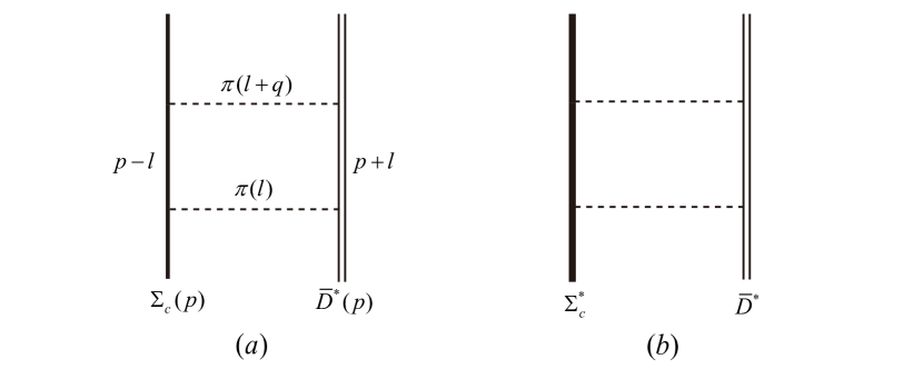
Figure 1: Two typical Feynman diagrams for the two-pion-exchange process of the $\Sigma_{c}\bar{D}^{\ast}$ ($a$) and $\Sigma_{c}^{\ast}\bar{D}^{\ast}$ ($b$) systems. We use the thick line, heavy-thick line, double-thin line and dashed line to denote the $\Sigma_{c}$, $\Sigma_{c}^{\ast}$, $\bar{D}^{\ast}$ and pion, respectively.

2 Effective chiral Lagrangians

In the framework of heavy hadron chiral perturbation theory, the scattering amplitudes of the $\Sigma_{c}^{(\ast)}\bar{D}^{(\ast)}$ systems can be expanded order by order in powers of a small parameter $\varepsilon=q/\Lambda_{\chi}$, where $q$ is either the momentum of Goldstone bosons or the residual momentum of heavy hadrons, and $\Lambda_{\chi}$ represents either the chiral breaking scale or the mass of a heavy hadron. The expansion is organized by the power counting rule Weinberg:1990rz ; Weinberg:1991um . One can get the order $\nu$ of a diagram with

$$\nu=2L-\frac{E_{n}}{2}+2+\sum_{i}V_{i}\Delta_{i},\quad\quad\Delta_{i}=d_{i}+\frac{n_{i}}{2}-2,$$ (1)

where $L$ and $E_{n}$ represent the number of loops and external lines of the matter field. $V_{i}$ denote the number of the type-$i$ vertex with the order $\Delta_{i}$. $d_{i}$ and $n_{i}$ stand for the number of derivatives (or $m_{\pi}$ factors) and external lines of the matter field in a type-$i$ vertex.

2.1 Pion interactions

In the SU(2) flavor space, the two light quarks in the charmed baryons can form the antisymmetric isosinglet and symmetric isotriplet. The corresponding total spins of the light quarks are $S_{l}=0$ and $S_{l}=1$, respectively. We use the notations $\psi_{1}$, $\psi_{3}$ and $\psi_{3^{\ast}}^{\mu}$ to denote the spin-$\frac{1}{2}$ isosinglet, spin-$\frac{1}{2}$ and spin-$\frac{3}{2}$ isotriplet, respectively.

$$\psi_{1}=\left(\begin{array}[]{cc}0&\Lambda_{c}^{+}\\ -\Lambda_{c}^{+}&0\end{array}\right),\quad\quad\psi_{3}=\left(\begin{array}[]{cc}\Sigma_{c}^{++}&\frac{\Sigma_{c}^{+}}{\sqrt{2}}\\ \frac{\Sigma_{c}^{+}}{\sqrt{2}}&\Sigma_{c}^{0}\end{array}\right),\quad\quad\psi_{3^{\ast}}^{\mu}=\left(\begin{array}[]{cc}\Sigma_{c}^{\ast++}&\frac{\Sigma_{c}^{\ast+}}{\sqrt{2}}\\ \frac{\Sigma_{c}^{\ast+}}{\sqrt{2}}&\Sigma_{c}^{\ast 0}\end{array}\right)^{\mu}.$$ (8)

The leading order relativistic chiral Lagrangians for the charmed baryons have been constructed in ref. Cheng:1992xi ; Liu:2012uw , which are given as

$$\mathcal{L}_{B\phi} = \mathrm{Tr}\left\{\bar{\psi}_{3^{\ast}}^{\mu}\left[-g_{\mu\nu}(i\not{D}-M_{3^{\ast}})+i(\gamma_{\mu}D_{\nu}+\gamma_{\nu}D_{\mu})-\gamma_{\mu}(i\not{D}+M_{3^{\ast}})\gamma_{\nu}\right]\psi_{3^{\ast}}^{\nu}\right\}$$ (9)

$$\mathrm{Tr}\left[\bar{\psi}_{3}(i\not{D}-M_{3})\psi_{3}\right]+g_{1}\mathrm{Tr}\left(\bar{\psi}_{3}\not{u}\gamma_{5}\psi_{3}\right)+g_{3}\mathrm{Tr}\left(\bar{\psi}_{3^{\ast}}^{\mu}u_{\mu}\psi_{3}+\mathrm{H.c.}\right)$$

$$+g_{5}\mathrm{Tr}\left(\bar{\psi}_{3^{\ast}}^{\mu}\not{u}\gamma_{5}\psi_{3^{\ast}\mu}\right)+\frac{1}{2}\mathrm{Tr}\left[\bar{\psi}_{1}(i\not{D}-M_{1})\psi_{1}\right]+g_{2}\mathrm{Tr}\left(\bar{\psi}_{3}\not{u}\gamma_{5}\psi_{1}+\mathrm{H.c.}\right)$$

$$+g_{4}\mathrm{Tr}\left(\bar{\psi}_{3^{\ast}}^{\mu}u_{\mu}\psi_{1}+\mathrm{H.c.}\right),$$

where $\mathrm{Tr}(X)$ denotes the trace of $X$ in flavor space. The covariant derivative $D_{\mu}$ is defined as $D_{\mu}\psi=\partial_{\mu}\psi+\Gamma_{\mu}\psi+\psi\Gamma_{\mu}^{T}$ ($\Gamma_{\mu}^{T}$ means the transposition of $\Gamma_{\mu}$). Meanwhile, the chiral connection $\Gamma_{\mu}$ and axial current $u_{\mu}$ are

$$\Gamma_{\mu} \equiv \frac{1}{2}\left[\xi^{\dagger},\partial_{\mu}\xi\right],\quad\quad\quad u_{\mu}\equiv\frac{i}{2}\left\{\xi^{\dagger},\partial_{\mu}\xi\right\},$$ (10)

where

$$\xi^{2}=U=\exp\left(\frac{i\phi}{f_{\pi}}\right),\quad\quad\quad\phi=\left(\begin{array}[]{cc}\pi^{0}&\sqrt{2}\pi^{+}\\ \sqrt{2}\pi^{-}&-\pi^{0}\end{array}\right),$$ (13)

and $f_{\pi}=92.4$ MeV is the pion decay constant.

We then adopt the heavy baryon reduction formalism Scherer:2002tk to get rid of the large baryon masses in eq. (9), where the heavy baryon field is decomposed into the light and heavy components by the projection operators $(1\pm\not{v})/2$,

$$\mathcal{B}_{i}=e^{iM_{i}v\cdot x}\frac{1+\not{v}}{2}\psi_{i},\quad\quad\quad\mathcal{H}_{i}=e^{iM_{i}v\cdot x}\frac{1-\not{v}}{2}\psi_{i},$$ (14)

where $\psi_{i}$ denotes the relativistic heavy baryon field $\psi_{1}$, $\psi_{3}$ and $\psi_{3^{\ast}}$, $M_{i}$ is their masses, and $v_{\mu}=(1,\mathbf{0})$ represents the four-velocity of a slowly moving heavy baryon. $\mathcal{B}_{i}$ and $\mathcal{H}_{i}$ are the corresponding light and heavy components, respectively. $\mathcal{H}_{i}$ disappears at the leading order expansion.

Consequently, the eq. (9) can then be reexpressed with the nonrelativistic form as

$$\mathcal{L}_{B\phi} = \mathrm{Tr}\left[\bar{\mathcal{B}}_{3}(iv\cdot D-\delta_{c})\mathcal{B}_{3}\right]-\mathrm{Tr}\left[\bar{\mathcal{B}}_{3^{\ast}}^{\mu}\left(iv\cdot D-\delta_{d}\right)\mathcal{B}_{3^{\ast}\mu}\right]+2g_{1}\mathrm{Tr}\left(\bar{\mathcal{B}}_{3}\mathcal{S}\cdot u\mathcal{B}_{3}\right)$$ (15)

$$+g_{3}\mathrm{Tr}\left(\bar{\mathcal{B}}_{3^{\ast}}^{\mu}u_{\mu}\mathcal{B}_{3}+\mathrm{H.c.}\right)+2g_{5}\mathrm{Tr}\left(\bar{\mathcal{B}}_{3^{\ast}}^{\mu}\mathcal{S}\cdot u\mathcal{B}_{3^{\ast}\mu}\right)+\frac{1}{2}\mathrm{Tr}\left[\bar{\mathcal{B}}_{1}(iv\cdot D)\mathcal{B}_{1}\right]$$

$$+2g_{2}\mathrm{Tr}\left(\bar{\mathcal{B}}_{3}\mathcal{S}\cdot u\mathcal{B}_{1}+\mathrm{H.c.}\right)+g_{4}\mathrm{Tr}\left(\bar{\mathcal{B}}_{3^{\ast}}^{\mu}u_{\mu}\mathcal{B}_{1}+\mathrm{H.c.}\right),$$

where $\mathcal{S}^{\mu}=\frac{i}{2}\gamma_{5}\sigma^{\mu\nu}v_{\nu}$ denotes the spin operator for the spin-$\frac{1}{2}$ particle. We adopt the mass splittings $\delta_{a}=M_{3^{\ast}}-M_{3}=65$ MeV, $\delta_{c}=M_{3}-M_{1}=168.5$ MeV, and $\delta_{d}=M_{3^{\ast}}-M_{1}=233.5$ MeV Tanabashi:2018oca .

Recall that the $(\psi_{3},\psi_{3^{\ast}})$ form the spin doublet in the heavy quark limit. Thus eq. (15) can be rewritten as a compact form by introducing the super-field Cheng:1993kp ; Cho:1992nt ,

$$\mathcal{L}_{B\phi} = -\mathrm{Tr}\left(\bar{\psi}^{\mu}iv\cdot D\psi_{\mu}\right)+ig_{a}\epsilon_{\mu\nu\rho\sigma}\mathrm{Tr}\left(\bar{\psi}^{\mu}u^{\rho}v^{\sigma}\psi^{\nu}\right)+i\frac{\delta_{a}}{2}\mathrm{Tr}\left(\bar{\psi}^{\mu}\sigma_{\mu\nu}\psi^{\nu}\right)$$ (16)

$$+\frac{1}{2}\mathrm{Tr}\left[\bar{\mathcal{B}}_{1}(iv\cdot D)\mathcal{B}_{1}\right]+g_{b}\mathrm{Tr}\left(\bar{\psi}^{\mu}u_{\mu}\mathcal{B}_{1}+\mathrm{H.c.}\right),$$

where the super-fields $\psi^{\mu}$ and $\bar{\psi}^{\mu}$ are defined as Cho:1992cf ; Cho:1992gg

$$\psi^{\mu}=\mathcal{B}_{3^{\ast}}^{\mu}-\frac{1}{\sqrt{3}}(\gamma^{\mu}+v^{\mu})\gamma^{5}\mathcal{B}_{3},\quad\quad\quad\bar{\psi}^{\mu}=\bar{\mathcal{B}}_{3^{\ast}}^{\mu}+\frac{1}{\sqrt{3}}\bar{\mathcal{B}}_{3}\gamma^{5}(\gamma^{\mu}+v^{\mu}).$$ (17)

Expanding eq. (16) and comparing them with the terms in eq. (15), one can get the relations among the different coupling constants,

$$g_{1}=-\frac{2}{3}g_{a},\quad g_{3}=-\frac{1}{\sqrt{3}}g_{a},\quad g_{5}=g_{a};\quad g_{2}=-\frac{1}{\sqrt{3}}g_{b},\quad g_{4}=g_{b}.$$ (18)

The values of $g_{2}$ and $g_{4}$ can be calculated with the partial decay widths of $\Sigma_{c}\to\Lambda_{c}\pi$ and $\Sigma_{c}^{\ast}\to\Lambda_{c}\pi$ Tanabashi:2018oca , respectively. The other axial couplings $g_{1}$, $g_{3}$ and $g_{5}$ can be obtained by their relations with $g_{2}$ in the framework of the quark model Meguro:2011nr ; Liu:2011xc ; Meng:2018gan , which yields

$$g_{2} =-0.60, \quad\quad\quad g_{4} =-\sqrt{3}g_{2}=1.04;$$

$$g_{1} =-\sqrt{\frac{8}{3}}g_{2}=0.98, \quad\quad\quad g_{3} =\frac{\sqrt{3}}{2}g_{1}=0.85, \quad\quad\quad g_{5}=-\frac{3}{2}g_{1}=-1.47.$$ (19)

The leading order chiral Lagrangians for the interactions between the anticharmed mesons and light pseudoscalars read Wise:1992hn ; Manohar:2000dt

$$\mathcal{L}_{H\phi}=-i\langle\bar{\tilde{\mathcal{H}}}v\cdot\mathcal{D}\tilde{\mathcal{H}}\rangle-\frac{1}{8}\delta_{b}\langle\bar{\tilde{\mathcal{H}}}\sigma^{\mu\nu}\tilde{\mathcal{H}}\sigma_{\mu\nu}\rangle+g\langle\bar{\tilde{\mathcal{H}}}\not{u}\gamma_{5}\tilde{\mathcal{H}}\rangle,$$ (20)

where $\langle X\rangle$ stands for the trace of $X$ in spinor space. The covariant derivative $\mathcal{D}_{\mu}=\partial_{\mu}+\Gamma_{\mu}$, $\delta_{b}=m_{\bar{D}^{\ast}}-m_{\bar{D}}$ is the mass splitting between $\bar{D}^{\ast}$ and $\bar{D}$. $g=-0.59$ represents the axial coupling constant, and its value is extracted from the partial decay width of $D^{\ast+}\to D^{0}\pi^{+}$ Tanabashi:2018oca , while the sign is determined by the quark model. We use the $\tilde{\mathcal{H}}$ to denote the super-field for the anticharmed mesons, which reads

$$\tilde{\mathcal{H}} = \left(\tilde{P}_{\mu}^{*}\gamma^{\mu}+i\tilde{P}\gamma_{5}\right)\frac{1-\not{v}}{2},\quad\quad\quad\bar{\tilde{\mathcal{H}}}=\gamma^{0}\tilde{\mathcal{H}}^{\dagger}\gamma^{0}=\frac{1-\not{v}}{2}\left(\tilde{P}_{\mu}^{*\dagger}\gamma^{\mu}+i\tilde{P}^{\dagger}\gamma_{5}\right),$$ (21)

where $\tilde{P}=(\bar{D}^{0},D^{-})^{T}$ and $\tilde{P}^{\ast}=(\bar{D}^{\ast 0},D^{\ast-})^{T}$, respectively.

2.2 Contact interactions

We then construct the leading order Lagrangians that account for the interactions between $\Sigma_{c}^{(\ast)}$ and $\bar{D}^{(\ast)}$ at the short range. We also use the super-field representations for $\Sigma_{c}^{(\ast)}$ and $\bar{D}^{(\ast)}$ to reduce the numbers of the LECs, which read Meng:2019ilv

$$\mathcal{L}_{HB} = D_{a}\langle\bar{\tilde{\mathcal{H}}}\tilde{\mathcal{H}}\rangle\mathrm{Tr}\big{(}\bar{\psi}^{\mu}\psi_{\mu}\big{)}+iD_{b}\epsilon_{\sigma\mu\nu\rho}v^{\sigma}\langle\bar{\tilde{\mathcal{H}}}\gamma^{\rho}\gamma_{5}\tilde{\mathcal{H}}\rangle\mathrm{Tr}\left(\bar{\psi}^{\mu}\psi^{\nu}\right)$$ (22)

$$+E_{a}\langle\bar{\tilde{\mathcal{H}}}\tau^{i}\tilde{\mathcal{H}}\rangle\mathrm{Tr}\big{(}\bar{\psi}^{\mu}\tau_{i}\psi_{\mu}\big{)}+iE_{b}\epsilon_{\sigma\mu\nu\rho}v^{\sigma}\langle\bar{\tilde{\mathcal{H}}}\gamma^{\rho}\gamma_{5}\tau^{i}\tilde{\mathcal{H}}\rangle\mathrm{Tr}\big{(}\bar{\psi}^{\mu}\tau_{i}\psi^{\nu}\big{)},$$

where the $D_{a}$, $D_{b}$, $E_{a}$ and $E_{b}$ are four independent LECs. The contact terms contain the residual contributions from the heavy degrees of freedom, which are integrated out and invisible at the low energy scale. Their values can be delicately determined from the experimental data Meng:2019ilv or roughly estimated with the theoretical models Xu:2017tsr ; Wang:2018atz . $D_{a}$ and $D_{b}$ contribute to the central potential and spin-spin interaction, respectively. $E_{a}$ and $E_{b}$ are related with the isospin-isospin interaction and contribute to the central and spin-spin interaction in spin space, respectively .

At the next-to-leading order, we need the $\mathcal{O}(\varepsilon^{2})$ LECs to absorb the divergences of the loop diagrams. These $\mathcal{O}(\varepsilon^{2})$ contact Lagrangians shall be proportional to the $m_{\pi}^{2}$, $\bm{q}^{2}$, $\delta_{a}^{2}$ and $\delta_{b}^{2}$. As demonstrated in ref. Liu:2012vd , there exist a large number of contact terms at $\mathcal{O}(\varepsilon^{2})$. It is very difficult to fix all these LECs at present. Therefore, in our work, we try to combine some contributions of the $\mathcal{O}(\varepsilon^{2})$ LECs with the leading ones by fitting the experimental data (At least the ones that proportional to $m_{\pi}^{2}$, $\delta_{a}^{2}$ and $\delta_{b}^{2}$ can be absorbed by renormalizing the $\mathcal{O}(\varepsilon^{0})$ LECs. The ones correlated with $\bm{q}^{2}$ can be largely compensated by the cutoff).

3 Analytical expressions for the effective potentials of the $\Sigma_{c}^{(\ast)}\bar{D}^{(\ast)}$ systems

The effective potential in momentum space can be obtained from the scattering amplitude in the following way Yang:2011wz ,

$$\mathcal{V}(\bm{q})=-\frac{\mathcal{M}(\bm{q})}{\sqrt{2M_{1}2M_{2}2M_{3}2M_{4}}},$$ (23)

where the $M_{1,2}$ and $M_{3,4}$ are the masses of the initial and final particles. The scattering amplitude $\mathcal{M}(\bm{q})$ is calculated by expanding the Lagrangians in eqs. (15), (20) and (22). Recall that at the leading order of the nonrelativistic expansions, there are the relations Manohar:2000dt

$$\psi(p)=\sqrt{2m_{\psi}}\left[\chi(v)+\mathcal{O}(1/m_{\psi})\right],\quad\quad\quad\tilde{\mathcal{H}}(p)=\sqrt{m_{H}}\left[\tilde{\mathcal{H}}(v)+\mathcal{O}(1/m_{H})\right],$$ (24)

where $\psi(p)$ and $\tilde{\mathcal{H}}(p)$ are the relativistic fields. $\chi(v)$ is the two-component spinor. The $\tilde{\mathcal{H}}(v)$ is the field in eqs. (20) and (22). We then make the Fourier transformation on $\mathcal{V}(\bm{q})$ to get the potential $\mathcal{V}(r)$ in the coordinate space,

$$\mathcal{V}(r)=\int\frac{d^{3}\bm{q}}{(2\pi)^{3}}e^{-i\bm{q\cdot r}}\mathcal{V}(\bm{q})\mathcal{F}(\bm{q}),$$ (25)

where the Gauss regulator $\mathcal{F}(\bm{q})=\exp\left(-\bm{q}^{2n}/\Lambda^{2n}\right)$ is introduced to regularize $\mathcal{V}(\bm{q})$ nonperturbatively Ordonez:1995rz ; Epelbaum:1999dj . As in refs. Xu:2017tsr ; Liu:2012vd ; Wang:2018atz ; Epelbaum:2014efa , we set $n=2$. The cutoff value $\Lambda$ is commonly chosen to be smaller than $\rho$ meson mass in the $N$-$N$ system Epelbaum:2014efa . We adopt a moderate value $\Lambda=0.5$ GeV as in ref. Meng:2019ilv .

3.1 $\Sigma_{c}\bar{D}$ system

Since the $\bar{D}\bar{D}\pi$ vertex is forbidden by the parity conservation law, the leading order effective potential for the $\Sigma_{c}\bar{D}$ system only arises from the contact terms [diagram $(X_{1.1})$ in the figure 2]. One can readily get

$$\mathcal{V}_{\Sigma_{c}\bar{D}}^{X_{1.1}}=-D_{a}-2E_{a}(\mathbf{I}_{1}\cdot\mathbf{I}_{2}),$$ (26)

where $\mathbf{I}_{1}$ and $\mathbf{I}_{2}$ represent the isospin operators of the $\Sigma_{c}^{(\ast)}$ and $\bar{D}^{(\ast)}$, respectively. The matrix element of $\mathbf{I}_{1}\cdot\mathbf{I}_{2}$ is

$$\langle\mathbf{I}_{1}\cdot\mathbf{I}_{2}\rangle=\left\{\begin{array}[]{ll}-1&\textrm{for $I=\frac{1}{2}$}\\ \frac{1}{2}&\textrm{for $I=\frac{3}{2}$}\end{array}\right.,$$

where $I$ is the total isospin of the $\Sigma_{c}^{(\ast)}\bar{D}^{(\ast)}$ system. The above values can be easily obtained with the relation $\langle\mathbf{I}_{1}\cdot\mathbf{I}_{2}\rangle=\frac{1}{2}\left[I(I+1)-I_{1}(I_{1}+1)-I_{2}(I_{2}+1)\right]$.

At the next-to-leading order, there are two types of one-loop diagrams. One is the two-pion-exchange diagrams is figure 3. Another one is the vertex corrections and wave function renormalizations in figure 4 Xu:2017tsr ; Liu:2012vd ; Wang:2018atz . The contribution of the diagrams in figure 4 could be included by using the physical values of the parameters in the Lagrangians, such as the pion mass, decay constant, coupling constants, etc..

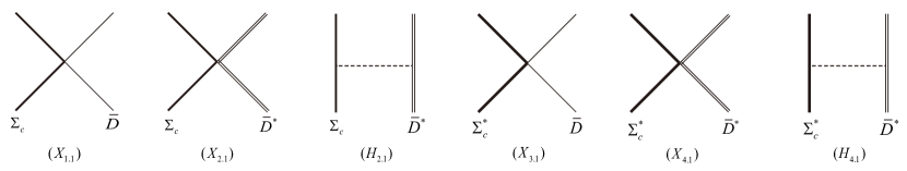
Figure 2: The leading order Feynman diagrams that account for the $\mathcal{O}(\varepsilon^{0})$ effective potentials of the $\Sigma_{c}\bar{D}$ ($X_{1.1}$), $\Sigma_{c}\bar{D}^{\ast}$ ($X_{2.1},H_{2.1}$), $\Sigma_{c}^{\ast}\bar{D}$ ($X_{3.1}$) and $\Sigma_{c}^{\ast}\bar{D}^{\ast}$ ($X_{4.1},H_{4,1}$) systems. We use the thin line to denote the $\bar{D}$ meson, and other notations are the same as those in figure 1.

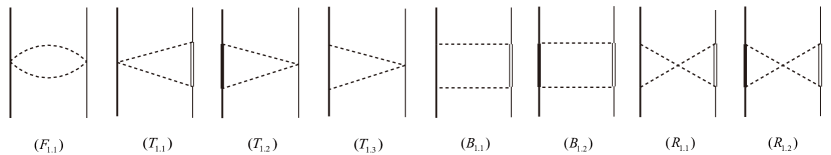
Figure 3: The two-pion-exchange diagrams of the $\Sigma_{c}\bar{D}$ system at $\mathcal{O}(\epsilon^{2})$. These diagrams are classified as the football diagram ($F_{1.1}$), triangle diagrams ($T_{1.i}$), box diagrams ($B_{1.i}$) and crossed box diagrams ($R_{1.i}$). The internal heavy baryon lines in diagrams $(T_{1.3})$, $(B_{1.1})$ and $(R_{1.1})$ can also be the $\Lambda_{c}$. The notations are the same as those in figure 2.

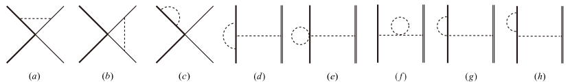
Figure 4: The next-to-leading order Feynman diagrams that contribute to the vertex corrections and wave function renormalizations. Each graph denotes the one type of diagrams with the same topological structure.

The analytical expressions of the two-pion-exchange diagrams in figure 3 read

$$\mathcal{V}_{\Sigma_{c}\bar{D}}^{F_{1.1}} = (\mathbf{I}_{1}\cdot\mathbf{I}_{2})\frac{1}{f_{\pi}^{4}}J_{22}^{F}(m_{\pi},q),$$ (27)

$$\mathcal{V}_{\Sigma_{c}\bar{D}}^{T_{1.1}} = (\mathbf{I}_{1}\cdot\mathbf{I}_{2})\frac{g^{2}}{f_{\pi}^{4}}\bigg{[}(d-1)J_{34}^{T}-\bm{q}^{2}\left(J_{24}^{T}+J_{33}^{T}\right)\bigg{]}(m_{\pi},\mathcal{E}-\delta_{b},q),$$ (28)

$$\mathcal{V}_{\Sigma_{c}\bar{D}}^{T_{1.2}} = (\mathbf{I}_{1}\cdot\mathbf{I}_{2})\frac{g_{3}^{2}}{4f_{\pi}^{4}}\bigg{[}(d-2)J_{34}^{T}-\bm{q}^{2}\frac{d-2}{d-1}\left(J_{24}^{T}+J_{33}^{T}\right)\bigg{]}(m_{\pi},\mathcal{E}-\delta_{a},q),$$ (29)

$$\mathcal{V}_{\Sigma_{c}\bar{D}}^{T_{1.3}} = (\mathbf{I}_{1}\cdot\mathbf{I}_{2})\frac{g_{1}^{2}}{4f_{\pi}^{4}}\bigg{[}(d-1)J_{34}^{T}-\bm{q}^{2}\left(J_{24}^{T}+J_{33}^{T}\right)\bigg{]}(m_{\pi},\mathcal{E},q),$$ (30)

$$\mathcal{V}_{\Sigma_{c}\bar{D}}^{B_{1.1}} = (1-\mathbf{I}_{1}\cdot\mathbf{I}_{2})\frac{g^{2}g_{1}^{2}}{8f_{\pi}^{4}}\bigg{[}(d^{2}-1)J_{41}^{B}-2\bm{q}^{2}(d+1)\left(J_{31}^{B}+J_{42}^{B}\right)-\bm{q}^{2}J_{21}^{B}$$ (31)

$$+\bm{q}^{4}\left(J_{22}^{B}+2J_{32}^{B}+J_{43}^{B}\right)\bigg{]}(m_{\pi},\mathcal{E},\mathcal{E}-\delta_{b},q),$$

$$\mathcal{V}_{\Sigma_{c}\bar{D}}^{B_{1.2}} = (1-\mathbf{I}_{1}\cdot\mathbf{I}_{2})\frac{g^{2}g_{3}^{2}}{8f_{\pi}^{4}}\bigg{[}(d^{2}-d-2)J_{41}^{B}-2\bm{q}^{2}\frac{d^{2}-d-2}{d-1}\left(J_{31}^{B}+J_{42}^{B}\right)-\bm{q}^{2}\frac{d-2}{d-1}J_{21}^{B}$$ (32)

$$+\bm{q}^{4}\frac{d-2}{d-1}\left(J_{22}^{B}+2J_{32}^{B}+J_{43}^{B}\right)\bigg{]}(m_{\pi},\mathcal{E}-\delta_{a},\mathcal{E}-\delta_{b},q),$$

$$\mathcal{V}_{\Sigma_{c}\bar{D}}^{R_{1.i}} = \mathcal{V}_{\Sigma_{c}\bar{D}}^{B_{1.i}}\Big{|}_{J_{x}^{B}\to J_{x}^{R},~{}\mathbf{I}_{1}\cdot\mathbf{I}_{2}\to-\mathbf{I}_{1}\cdot\mathbf{I}_{2}}.$$ (33)

When the contribution of $\Lambda_{c}$ is included, it will appear in the graphs $(T_{1.3})$, $(B_{1.1})$ and $(R_{1.1})$ as the intermediate state. The expressions read (we use $\bar{T}_{i.j}$, $\bar{B}_{i.j}$ and $\bar{R}_{i.j}$ to denote the loops with $\Lambda_{c}$)

$$\mathcal{V}_{\Sigma_{c}\bar{D}}^{\bar{T}_{1.3}} = (\mathbf{I}_{1}\cdot\mathbf{I}_{2})\frac{g_{2}^{2}}{2f_{\pi}^{4}}\bigg{[}(d-1)J_{34}^{T}-\bm{q}^{2}\left(J_{24}^{T}+J_{33}^{T}\right)\bigg{]}(m_{\pi},\mathcal{E}+\delta_{c},q),$$ (34)

$$\mathcal{V}_{\Sigma_{c}\bar{D}}^{\bar{B}_{1.1}} = (1-2\mathbf{I}_{1}\cdot\mathbf{I}_{2})\frac{g^{2}g_{2}^{2}}{8f_{\pi}^{4}}\bigg{[}(d^{2}-1)J_{41}^{B}-2\bm{q}^{2}(d+1)\left(J_{31}^{B}+J_{42}^{B}\right)-\bm{q}^{2}J_{21}^{B}$$ (35)

$$+\bm{q}^{4}\left(J_{22}^{B}+2J_{32}^{B}+J_{43}^{B}\right)\bigg{]}(m_{\pi},\mathcal{E}+\delta_{c},\mathcal{E}-\delta_{b},q),$$

$$\mathcal{V}_{\Sigma_{c}\bar{D}}^{\bar{R}_{1.1}} = \mathcal{V}_{\Sigma_{c}\bar{D}}^{\bar{B}_{1.1}}\Big{|}_{J_{x}^{B}\to J_{x}^{R},~{}\mathbf{I}_{1}\cdot\mathbf{I}_{2}\to-\mathbf{I}_{1}\cdot\mathbf{I}_{2}}.$$ (36)

In above equations, the loop functions $J_{x}^{y}$ are defined in appendix A. $d$ is the dimension where the loop integral is performed and approaches four at last. $\mathcal{E}$ represents the residual energies of the $\Sigma_{c}^{(\ast)}$ and $\bar{D}^{(\ast)}$, which is defined as $\mathcal{E}=E_{i}-M_{i}~{}(i=\Sigma_{c}^{(\ast)},\bar{D}^{(\ast)})$. $\mathcal{E}$ is set to zero in our calculations.

3.2 $\Sigma_{c}\bar{D}^{\ast}$ system

The leading order potential for the $\Sigma_{c}\bar{D}^{\ast}$ system stems from the contact interaction and one-pion-exchange diagrams [graphs $(X_{2.1})$ and $(H_{2.1})$ in figure 2], which reads

$$\mathcal{V}_{\Sigma_{c}\bar{D}^{\ast}}^{X_{2.1}} = -D_{a}-2E_{a}(\mathbf{I}_{1}\cdot\mathbf{I}_{2})+\frac{2}{3}\Big{[}-D_{b}-2E_{b}(\mathbf{I}_{1}\cdot\mathbf{I}_{2})\Big{]}\bm{\sigma}\cdot\bm{T},$$ (37)

$$\mathcal{V}_{\Sigma_{c}\bar{D}^{\ast}}^{H_{2.1}} = -(\mathbf{I}_{1}\cdot\mathbf{I}_{2})\frac{gg_{1}}{2f_{\pi}^{2}}\frac{(\bm{q}\cdot\bm{\sigma})(\bm{q}\cdot\bm{T})}{\bm{q}^{2}+m_{\pi}^{2}},$$ (38)

where $\bm{\sigma}$ is the Pauli matrix. The spin operator $\bm{S}_{1}$ of $\Sigma_{c}$ satisfies $\bm{S}_{1}=\frac{1}{2}\bm{\sigma}$. The operator $\bm{T}=i\bm{\varepsilon}^{\ast}\times\bm{\varepsilon}$ ($\bm{\varepsilon}$ and $\bm{\varepsilon}^{\ast}$ are the space components of polarization vectors of the initial and final $\bar{D}^{\ast}$ meson) is correlated with the spin operator $\bm{S}_{2}$ of the $\bar{D}^{\ast}$ meson by the relation $\bm{S}_{2}=-\bm{T}$. Thus the $\bm{\sigma}\cdot\bm{T}$ term represents the spin-spin interaction (see appendix C). Since only the $S$-wave interaction is considered, one can use the following replacement rules in the potentials,

$$\bm{\varepsilon}^{\ast}\cdot\bm{\varepsilon}\longmapsto 1,\quad\quad\quad q_{i}q_{j}\longmapsto\frac{1}{d-1}\bm{q}^{2}\delta_{ij}.$$ (39)

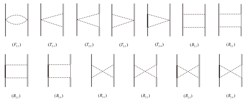
Figure 5: The two-pion-exchange diagrams of the $\Sigma_{c}\bar{D}^{\ast}$ system at $\mathcal{O}(\epsilon^{2})$. The internal heavy baryon lines in diagrams $(T_{2.3})$, $(B_{2.1})$, $(B_{2.2})$, $(R_{2.1})$ and $(R_{2.2})$ can also be the $\Lambda_{c}$. The notations are the same as those in figure 2.

The two-pion-exchange diagrams for the $\Sigma_{c}\bar{D}^{\ast}$ system are shown in figure 5. The potentials from these graphs read

$$\mathcal{V}_{\Sigma_{c}\bar{D}^{\ast}}^{F_{2.1}} = (\mathbf{I}_{1}\cdot\mathbf{I}_{2})\frac{1}{f_{\pi}^{4}}J_{22}^{F}(m_{\pi},q),$$ (40)

$$\mathcal{V}_{\Sigma_{c}\bar{D}^{\ast}}^{T_{2.1}} = (\mathbf{I}_{1}\cdot\mathbf{I}_{2})\frac{g^{2}}{f_{\pi}^{4}}\left[2J_{34}^{T}-\bm{q}^{2}\frac{d-2}{d-1}\left(J_{24}^{T}+J_{33}^{T}\right)\right](m_{\pi},\mathcal{E},q),$$ (41)

$$\mathcal{V}_{\Sigma_{c}\bar{D}^{\ast}}^{T_{2.2}} = (\mathbf{I}_{1}\cdot\mathbf{I}_{2})\frac{g^{2}}{f_{\pi}^{4}}\left[J_{34}^{T}-\frac{\bm{q}^{2}}{d-1}\left(J_{24}^{T}+J_{33}^{T}\right)\right](m_{\pi},\mathcal{E}+\delta_{b},q),$$ (42)

$$\mathcal{V}_{\Sigma_{c}\bar{D}^{\ast}}^{T_{2.3}} = (\mathbf{I}_{1}\cdot\mathbf{I}_{2})\frac{g_{1}^{2}}{4f_{\pi}^{4}}\bigg{[}(d-1)J_{34}^{T}-\bm{q}^{2}\left(J_{24}^{T}+J_{33}^{T}\right)\bigg{]}(m_{\pi},\mathcal{E},q),$$ (43)

$$\mathcal{V}_{\Sigma_{c}\bar{D}^{\ast}}^{T_{2.4}} = (\mathbf{I}_{1}\cdot\mathbf{I}_{2})\frac{g_{3}^{2}}{4f_{\pi}^{4}}\bigg{[}(d-2)J_{34}^{T}-\bm{q}^{2}\frac{d-2}{d-1}\left(J_{24}^{T}+J_{33}^{T}\right)\bigg{]}(m_{\pi},\mathcal{E}-\delta_{a},q),$$ (44)

$$\mathcal{V}_{\Sigma_{c}\bar{D}^{\ast}}^{B_{2.1}} = (1-\mathbf{I}_{1}\cdot\mathbf{I}_{2})\frac{g^{2}g_{1}^{2}}{8f_{\pi}^{4}}\bigg{[}\frac{4d^{2}-10d+6}{d-1}J_{41}^{B}-\bm{q}^{2}\frac{d^{2}+3d-8}{d-1}\left(J_{31}^{B}+J_{42}^{B}\right)$$ (45)

$$-\bm{q}^{2}\frac{d-2+\bm{\sigma}\cdot\bm{T}}{d-1}J_{21}^{B}+\bm{q}^{4}\frac{d-2}{d-1}\left(J_{22}^{B}+2J_{32}^{B}+J_{43}^{B}\right)\bigg{]}(m_{\pi},\mathcal{E},\mathcal{E},q),$$

$$\mathcal{V}_{\Sigma_{c}\bar{D}^{\ast}}^{B_{2.2}} = (1-\mathbf{I}_{1}\cdot\mathbf{I}_{2})\frac{g^{2}g_{1}^{2}}{8f_{\pi}^{4}}\bigg{[}-2\bm{q}^{2}\frac{d+1}{d-1}\left(J_{31}^{B}+J_{42}^{B}\right)-\bm{q}^{2}\frac{1}{d-1}(1+\bm{\sigma}\cdot\bm{T})J_{21}^{B}$$ (46)

$$+(d+1)J_{41}^{B}+\bm{q}^{4}\frac{1}{d-1}\left(J_{22}^{B}+2J_{32}^{B}+J_{43}^{B}\right)\bigg{]}(m_{\pi},\mathcal{E},\mathcal{E}+\delta_{b},q),$$

$$\mathcal{V}_{\Sigma_{c}\bar{D}^{\ast}}^{B_{2.3}} = (1-\mathbf{I}_{1}\cdot\mathbf{I}_{2})\frac{g^{2}g_{3}^{2}}{8f_{\pi}^{4}}\bigg{[}-\bm{q}^{2}\frac{(d-2)^{2}-\bm{\sigma}\cdot\bm{T}}{(d-1)^{2}}J_{21}^{B}-\bm{q}^{2}\frac{(d-2)(d^{2}+3d-8)}{(d-1)^{2}}\left(J_{31}^{B}+J_{42}^{B}\right)$$ (47)

$$+\frac{2(d^{2}-2d+2)}{d-1}J_{41}^{B}+\bm{q}^{4}\frac{(d-2)^{2}}{(d-1)^{2}}\left(J_{22}^{B}+2J_{32}^{B}+J_{43}^{B}\right)\bigg{]}(m_{\pi},\mathcal{E}-\delta_{a},\mathcal{E},q),$$

$$\mathcal{V}_{\Sigma_{c}\bar{D}^{\ast}}^{B_{2.4}} = (1-\mathbf{I}_{1}\cdot\mathbf{I}_{2})\frac{g^{2}g_{3}^{2}}{8f_{\pi}^{4}}\frac{1}{d-1}\bigg{[}-2\bm{q}^{2}\frac{(d+1)(d-2)}{d-1}\left(J_{31}^{B}+J_{42}^{B}\right)-\bm{q}^{2}\frac{d-2-\bm{\sigma}\cdot\bm{T}}{d-1}J_{21}^{B}$$ (48)

$$+\bm{q}^{4}\frac{d-2}{d-1}\left(J_{22}^{B}+2J_{32}^{B}+J_{43}^{B}\right)+(d^{2}-d-2)J_{41}^{B}\bigg{]}(m_{\pi},\mathcal{E}-\delta_{a},\mathcal{E}+\delta_{b},q),$$

$$\mathcal{V}_{\Sigma_{c}\bar{D}^{\ast}}^{R_{2.i}} = \mathcal{V}_{\Sigma_{c}\bar{D}^{\ast}}^{B_{2.i}}\Big{|}_{J_{x}^{B}\to J_{x}^{R},~{}\mathbf{I}_{1}\cdot\mathbf{I}_{2}\to-\mathbf{I}_{1}\cdot\mathbf{I}_{2},~{}\bm{\sigma}\cdot\bm{T}\to-\bm{\sigma}\cdot\bm{T}}.$$ (49)

Considering the contribution of $\Lambda_{c}$:

$$\mathcal{V}_{\Sigma_{c}\bar{D}^{\ast}}^{\bar{T}_{2.3}} = (\mathbf{I}_{1}\cdot\mathbf{I}_{2})\frac{g_{2}^{2}}{2f_{\pi}^{4}}\bigg{[}(d-1)J_{34}^{T}-\bm{q}^{2}\left(J_{24}^{T}+J_{33}^{T}\right)\bigg{]}(m_{\pi},\mathcal{E}+\delta_{c},q),$$ (50)

$$\mathcal{V}_{\Sigma_{c}\bar{D}^{\ast}}^{\bar{B}_{2.1}} = (1-2\mathbf{I}_{1}\cdot\mathbf{I}_{2})\frac{g^{2}g_{2}^{2}}{8f_{\pi}^{4}}\bigg{[}\frac{4d^{2}-10d+6}{d-1}J_{41}^{B}-\bm{q}^{2}\frac{d^{2}+3d-8}{d-1}\left(J_{31}^{B}+J_{42}^{B}\right)$$ (51)

$$-\bm{q}^{2}\frac{d-2+\bm{\sigma}\cdot\bm{T}}{d-1}J_{21}^{B}+\bm{q}^{4}\frac{d-2}{d-1}\left(J_{22}^{B}+2J_{32}^{B}+J_{43}^{B}\right)\bigg{]}(m_{\pi},\mathcal{E}+\delta_{c},\mathcal{E},q),$$

$$\mathcal{V}_{\Sigma_{c}\bar{D}^{\ast}}^{\bar{B}_{2.2}} = (1-2\mathbf{I}_{1}\cdot\mathbf{I}_{2})\frac{g^{2}g_{2}^{2}}{8f_{\pi}^{4}}\bigg{[}-2\bm{q}^{2}\frac{d+1}{d-1}\left(J_{31}^{B}+J_{42}^{B}\right)-\bm{q}^{2}\frac{1}{d-1}(1+\bm{\sigma}\cdot\bm{T})J_{21}^{B}$$ (52)

$$+(d+1)J_{41}^{B}+\bm{q}^{4}\frac{1}{d-1}\left(J_{22}^{B}+2J_{32}^{B}+J_{43}^{B}\right)\bigg{]}(m_{\pi},\mathcal{E}+\delta_{c},\mathcal{E}+\delta_{b},q),$$

$$\mathcal{V}_{\Sigma_{c}\bar{D}^{\ast}}^{\bar{R}_{2.i}} = \mathcal{V}_{\Sigma_{c}\bar{D}^{\ast}}^{\bar{B}_{2.i}}\Big{|}_{J_{x}^{B}\to J_{x}^{R},~{}\mathbf{I}_{1}\cdot\mathbf{I}_{2}\to-\mathbf{I}_{1}\cdot\mathbf{I}_{2},~{}\bm{\sigma}\cdot\bm{T}\to-\bm{\sigma}\cdot\bm{T}}.$$ (53)

From the above equations we see that, in the $S$-wave interactions, only the central terms and spin-spin interactions survive in the effective potentials.

3.3 $\Sigma_{c}^{\ast}\bar{D}$ system

Like the $\Sigma_{c}\bar{D}$ system, the leading order potential for the $\Sigma_{c}^{\ast}\bar{D}$ system only stems from the contact terms [diagram $(X_{3.1})$ in figure 2]. The expression reads

$$\mathcal{V}_{\Sigma_{c}^{\ast}\bar{D}}^{X_{3.1}}=-D_{a}-2E_{a}(\mathbf{I}_{1}\cdot\mathbf{I}_{2}).$$ (54)

We see that the contact potential of the $\Sigma_{c}^{\ast}\bar{D}$ system equals to the one of the $\Sigma_{c}\bar{D}$ system in eq. (26), because the $\mathcal{O}(\varepsilon^{0})$ contact Lagrangian is constructed in the heavy quark limit. The heavy quark breaking effect will be manifested in the loop diagrams when the mass splittings are considered in the propagators of the heavy matter fields.

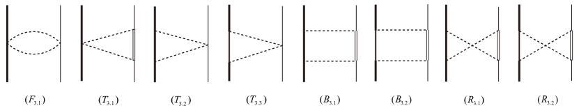
Figure 6: The two-pion-exchange diagrams of the $\Sigma_{c}^{\ast}\bar{D}$ system at $\mathcal{O}(\epsilon^{2})$. The internal heavy baryon lines in diagrams $(T_{3.3})$, $(B_{3.2})$ and $(R_{3.2})$ can also be the $\Lambda_{c}$. The notations are the same as those in figure 2.

The two-pion-exchange diagrams are illustrated in figure 6. The analytical results for these diagrams are given as

$$\mathcal{V}_{\Sigma_{c}^{\ast}\bar{D}}^{F_{3.1}} = (\mathbf{I}_{1}\cdot\mathbf{I}_{2})\frac{1}{f_{\pi}^{4}}J_{22}^{F}(m_{\pi},q),$$ (55)

$$\mathcal{V}_{\Sigma_{c}^{\ast}\bar{D}}^{T_{3.1}} = (\mathbf{I}_{1}\cdot\mathbf{I}_{2})\frac{g^{2}}{f_{\pi}^{4}}\bigg{[}(d-1)J_{34}^{T}-\bm{q}^{2}\left(J_{24}^{T}+J_{33}^{T}\right)\bigg{]}(m_{\pi},\mathcal{E}-\delta_{b},q),$$ (56)

$$\mathcal{V}_{\Sigma_{c}^{\ast}\bar{D}}^{T_{3.2}} = (\mathbf{I}_{1}\cdot\mathbf{I}_{2})\frac{g_{5}^{2}}{4f_{\pi}^{4}}\frac{d^{2}-2d-3}{(d-1)^{2}}\bigg{[}(d-1)J_{34}^{T}-\bm{q}^{2}\left(J_{24}^{T}+J_{33}^{T}\right)\bigg{]}(m_{\pi},\mathcal{E},q),$$ (57)

$$\mathcal{V}_{\Sigma_{c}^{\ast}\bar{D}}^{T_{3.3}} = (\mathbf{I}_{1}\cdot\mathbf{I}_{2})\frac{g_{3}^{2}}{4f_{\pi}^{4}}\bigg{[}J_{34}^{T}-\frac{\bm{q}^{2}}{d-1}\left(J_{24}^{T}+J_{33}^{T}\right)\bigg{]}(m_{\pi},\mathcal{E}+\delta_{a},q),$$ (58)

$$\mathcal{V}_{\Sigma_{c}^{\ast}\bar{D}}^{B_{3.1}} = (1-\mathbf{I}_{1}\cdot\mathbf{I}_{2})\frac{g^{2}g_{5}^{2}}{8f_{\pi}^{4}}\frac{d^{2}-2d-3}{(d-1)^{2}}\bigg{[}(d^{2}-1)J_{41}^{B}-2\bm{q}^{2}(d+1)\left(J_{31}^{B}+J_{42}^{B}\right)$$ (59)

$$-\bm{q}^{2}J_{21}^{B}+\bm{q}^{4}\left(J_{22}^{B}+2J_{32}^{B}+J_{43}^{B}\right)\bigg{]}(m_{\pi},\mathcal{E},\mathcal{E}-\delta_{b},q),$$

$$\mathcal{V}_{\Sigma_{c}^{\ast}\bar{D}}^{B_{3.2}} = (1-\mathbf{I}_{1}\cdot\mathbf{I}_{2})\frac{g^{2}g_{3}^{2}}{8f_{\pi}^{4}}\bigg{[}(d+1)J_{41}^{B}-2\bm{q}^{2}\frac{d+1}{d-1}\left(J_{31}^{B}+J_{42}^{B}\right)-\bm{q}^{2}\frac{1}{d-1}J_{21}^{B}$$ (60)

$$+\bm{q}^{4}\frac{1}{d-1}\left(J_{22}^{B}+2J_{32}^{B}+J_{43}^{B}\right)\bigg{]}(m_{\pi},\mathcal{E}+\delta_{a},\mathcal{E}-\delta_{b},q),$$

$$\mathcal{V}_{\Sigma_{c}^{\ast}\bar{D}}^{R_{3.i}} = \mathcal{V}_{\Sigma_{c}^{\ast}\bar{D}}^{B_{3.i}}\Big{|}_{J_{x}^{B}\to J_{x}^{R},~{}\mathbf{I}_{1}\cdot\mathbf{I}_{2}\to-\mathbf{I}_{1}\cdot\mathbf{I}_{2}}.$$ (61)

Including the contribution of $\Lambda_{c}$:

$$\mathcal{V}_{\Sigma_{c}^{\ast}\bar{D}}^{\bar{T}_{3.3}} = (\mathbf{I}_{1}\cdot\mathbf{I}_{2})\frac{g_{4}^{2}}{2f_{\pi}^{4}}\bigg{[}J_{34}^{T}-\frac{\bm{q}^{2}}{d-1}\left(J_{24}^{T}+J_{33}^{T}\right)\bigg{]}(m_{\pi},\mathcal{E}+\delta_{d},q),$$ (62)

$$\mathcal{V}_{\Sigma_{c}^{\ast}\bar{D}}^{\bar{B}_{3.2}} = (1-2\mathbf{I}_{1}\cdot\mathbf{I}_{2})\frac{g^{2}g_{4}^{2}}{8f_{\pi}^{4}}\bigg{[}(d+1)J_{41}^{B}-2\bm{q}^{2}\frac{d+1}{d-1}\left(J_{31}^{B}+J_{42}^{B}\right)-\bm{q}^{2}\frac{1}{d-1}J_{21}^{B}$$ (63)

$$+\bm{q}^{4}\frac{1}{d-1}\left(J_{22}^{B}+2J_{32}^{B}+J_{43}^{B}\right)\bigg{]}(m_{\pi},\mathcal{E}+\delta_{d},\mathcal{E}-\delta_{b},q),$$

$$\mathcal{V}_{\Sigma_{c}^{\ast}\bar{D}}^{\bar{R}_{3.2}} = V_{\Sigma_{c}^{\ast}\bar{D}}^{\bar{B}_{3.2}}\Big{|}_{J_{x}^{B}\to J_{x}^{R},~{}\mathbf{I}_{1}\cdot\mathbf{I}_{2}\to-\mathbf{I}_{1}\cdot\mathbf{I}_{2}}.$$ (64)

3.4 $\Sigma_{c}^{\ast}\bar{D}^{\ast}$ system

The leading order diagrams for $\Sigma_{c}^{\ast}\bar{D}^{\ast}$ system are the graphs $(X_{4.1})$ and $(H_{4.1})$ in figure 2. The potentials from these two graphs read

$$\mathcal{V}_{\Sigma_{c}^{\ast}\bar{D}^{\ast}}^{X_{4.1}} = -D_{a}-2E_{a}(\mathbf{I}_{1}\cdot\mathbf{I}_{2})+\Big{[}-D_{b}-2E_{b}(\mathbf{I}_{1}\cdot\mathbf{I}_{2})\Big{]}\bm{\sigma}_{rs}\cdot\bm{T},$$ (65)

$$\mathcal{V}_{\Sigma_{c}^{\ast}\bar{D}^{\ast}}^{H_{4.1}} = (\mathbf{I}_{1}\cdot\mathbf{I}_{2})\frac{gg_{5}}{2f_{\pi}^{2}}\frac{(\bm{q}\cdot\bm{\sigma}_{rs})(\bm{q}\cdot\bm{T})}{\bm{q}^{2}+m_{\pi}^{2}},$$ (66)

where the operator $\bm{\sigma}_{rs}$ is related to the spin operator $\bm{S}_{1}$ of the $\Sigma_{c}^{\ast}$ with $\bm{S}_{1}=\frac{3}{2}\bm{\sigma}_{rs}$ (see the detailed derivations in appendix C), so the $\bm{\sigma}_{rs}\cdot\bm{T}$ term represents the spin-spin interaction as well. We see the $\mathcal{O}(\varepsilon^{0})$ potentials for $\Sigma_{c}^{\ast}\bar{D}^{\ast}$ resemble the ones for $\Sigma_{c}\bar{D}^{\ast}$ in eqs. (37) and (38).

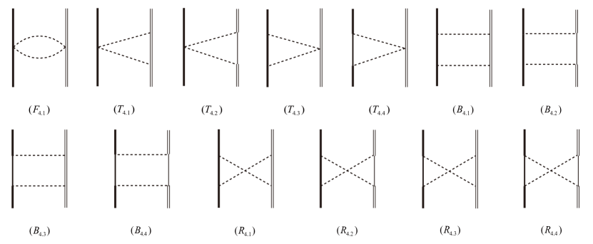
Figure 7: The two-pion-exchange diagrams of the $\Sigma_{c}^{\ast}\bar{D}^{\ast}$ system at $\mathcal{O}(\epsilon^{2})$. The internal heavy baryon lines in diagrams $(T_{4.4})$, $(B_{4.3})$, $(B_{4.4})$, $(R_{4.3})$ and $(R_{4.4})$ can also be the $\Lambda_{c}$. The notations are the same as those in figure 2.

The two-pion-exchange diagrams are displayed in figure 7. The potentials originate from these graphs read

$$\mathcal{V}_{\Sigma_{c}^{\ast}\bar{D}^{\ast}}^{F_{4.1}} = (\mathbf{I}_{1}\cdot\mathbf{I}_{2})\frac{1}{f_{\pi}^{4}}J_{22}^{F}(m_{\pi},q),$$ (67)

$$\mathcal{V}_{\Sigma_{c}^{\ast}\bar{D}^{\ast}}^{T_{4.1}} = (\mathbf{I}_{1}\cdot\mathbf{I}_{2})\frac{g^{2}}{f_{\pi}^{4}}\bigg{[}2J_{34}^{T}-\bm{q}^{2}\frac{d-2}{d-1}\left(J_{24}^{T}+J_{33}^{T}\right)\bigg{]}(m_{\pi},\mathcal{E},q),$$ (68)

$$\mathcal{V}_{\Sigma_{c}^{\ast}\bar{D}^{\ast}}^{T_{4.2}} = (\mathbf{I}_{1}\cdot\mathbf{I}_{2})\frac{g^{2}}{f_{\pi}^{4}}\bigg{[}J_{34}^{T}-\frac{\bm{q}^{2}}{d-1}\left(J_{24}^{T}+J_{33}^{T}\right)\bigg{]}(m_{\pi},\mathcal{E}+\delta_{b},q),$$ (69)

$$\mathcal{V}_{\Sigma_{c}^{\ast}\bar{D}^{\ast}}^{T_{4.3}} = (\mathbf{I}_{1}\cdot\mathbf{I}_{2})\frac{g_{5}^{2}}{4f_{\pi}^{4}}\frac{d^{2}-2d-3}{(d-1)^{2}}\bigg{[}(d-1)J_{34}^{T}-\bm{q}^{2}\left(J_{24}^{T}+J_{33}^{T}\right)\bigg{]}(m_{\pi},\mathcal{E},q),$$ (70)

$$\mathcal{V}_{\Sigma_{c}^{\ast}\bar{D}^{\ast}}^{T_{4.4}} = (\mathbf{I}_{1}\cdot\mathbf{I}_{2})\frac{g_{3}^{2}}{4f_{\pi}^{4}}\bigg{[}J_{34}^{T}-\frac{\bm{q}^{2}}{d-1}\left(J_{24}^{T}+J_{33}^{T}\right)\bigg{]}(m_{\pi},\mathcal{E}+\delta_{a},q),$$ (71)

$$\mathcal{V}_{\Sigma_{c}^{\ast}\bar{D}^{\ast}}^{B_{4.1}} = (1-\mathbf{I}_{1}\cdot\mathbf{I}_{2})\frac{g^{2}g_{5}^{2}}{8f_{\pi}^{4}}\frac{1}{d-1}\Bigg{[}2\left(2d^{2}-5d-7+3(\bm{\sigma}_{rs}\cdot\bm{T})^{2}-\bm{\sigma}_{rs}\cdot\bm{T}\right)J_{41}^{B}$$ (72)

$$-\bm{q}^{2}\frac{d^{3}+2d^{2}-15d-16+12(\bm{\sigma}_{rs}\cdot\bm{T})^{2}-4\bm{\sigma}_{rs}\cdot\bm{T}}{d-1}\left(J_{31}^{B}+J_{42}^{B}\right)$$

$$-\bm{q}^{2}\frac{d^{2}-3d-4+3(\bm{\sigma}_{rs}\cdot\bm{T})^{2}+(d-4)\bm{\sigma}_{rs}\cdot\bm{T}}{d-1}J_{21}^{B}$$

$$+\bm{q}^{4}\frac{d^{3}-4d^{2}+d+6}{(d-1)^{2}}\left(J_{22}^{B}+2J_{32}^{B}+J_{43}^{B}\right)\Bigg{]}(m_{\pi},\mathcal{E},\mathcal{E},q),$$

$$\mathcal{V}_{\Sigma_{c}^{\ast}\bar{D}^{\ast}}^{B_{4.2}} = (1-\mathbf{I}_{1}\cdot\mathbf{I}_{2})\frac{g^{2}g_{5}^{2}}{8f_{\pi}^{4}}\frac{1}{d-1}\Bigg{[}\left(d^{2}-1-6(\bm{\sigma}_{rs}\cdot\bm{T})^{2}+2\bm{\sigma}_{rs}\cdot\bm{T}\right)J_{41}^{B}+\bm{q}^{4}\frac{d^{2}-2d-3}{(d-1)^{2}}$$ (73)

$$\times\left(J_{22}^{B}+2J_{32}^{B}+J_{43}^{B}\right)-2\bm{q}^{2}\frac{d^{2}-1-6(\bm{\sigma}_{rs}\cdot\bm{T})^{2}+2\bm{\sigma}_{rs}\cdot\bm{T}}{d-1}\left(J_{31}^{B}+J_{42}^{B}\right)$$

$$-\bm{q}^{2}\frac{d+1-3(\bm{\sigma}_{rs}\cdot\bm{T})^{2}+(d-2)\bm{\sigma}_{rs}\cdot\bm{T}}{d-1}J_{21}^{B}\Bigg{]}(m_{\pi},\mathcal{E},\mathcal{E}+\delta_{b},q),$$

$$\mathcal{V}_{\Sigma_{c}^{\ast}\bar{D}^{\ast}}^{B_{4.3}} = (1-\mathbf{I}_{1}\cdot\mathbf{I}_{2})\frac{g^{2}g_{3}^{2}}{32f_{\pi}^{4}}\Bigg{[}\left(20-6(\bm{\sigma}_{rs}\cdot\bm{T})^{2}+2\bm{\sigma}_{rs}\cdot\bm{T}\right)J_{41}^{B}+4\bm{q}^{4}\frac{d-2}{(d-1)^{2}}\big{(}J_{22}^{B}$$ (74)

$$+2J_{32}^{B}+J_{43}^{B}\big{)}-4\bm{q}^{2}\frac{d+6-3(\bm{\sigma}_{rs}\cdot\bm{T})^{2}+\bm{\sigma}_{rs}\cdot\bm{T}}{d-1}\left(J_{31}^{B}+J_{42}^{B}\right)$$

$$+3\bm{q}^{2}\frac{(\bm{\sigma}_{rs}\cdot\bm{T})^{2}-\bm{\sigma}_{rs}\cdot\bm{T}-2}{d-1}J_{21}^{B}\Bigg{]}(m_{\pi},\mathcal{E}+\delta_{a},\mathcal{E},q),$$

$$\mathcal{V}_{\Sigma_{c}^{\ast}\bar{D}^{\ast}}^{B_{4.4}} = (1-\mathbf{I}_{1}\cdot\mathbf{I}_{2})\frac{g^{2}g_{3}^{2}}{32f_{\pi}^{4}}\Bigg{[}\left(6(\bm{\sigma}_{rs}\cdot\bm{T})^{2}-2\bm{\sigma}_{rs}\cdot\bm{T}\right)J_{41}^{B}+4\bm{q}^{2}\frac{-3(\bm{\sigma}_{rs}\cdot\bm{T})^{2}+\bm{\sigma}_{rs}\cdot\bm{T}}{d-1}$$ (75)

$$\times\left(J_{31}^{B}+J_{42}^{B}\right)+4\bm{q}^{4}\frac{1}{(d-1)^{2}}\left(J_{22}^{B}+2J_{32}^{B}+J_{43}^{B}\right)$$

$$-\bm{q}^{2}\frac{3(\bm{\sigma}_{rs}\cdot\bm{T})^{2}+\bm{\sigma}_{rs}\cdot\bm{T}-2}{d-1}J_{21}^{B}\Bigg{]}(m_{\pi},\mathcal{E}+\delta_{a},\mathcal{E}+\delta_{b},q).$$

Unlike the two-pion-exchange potentials of the $\Sigma_{c}\bar{D}^{\ast}$ system, there exists a very simple relation between $\mathcal{V}_{\Sigma_{c}\bar{D}^{\ast}}^{R_{2.i}}$ and $\mathcal{V}_{\Sigma_{c}\bar{D}^{\ast}}^{B_{2.i}}$ [e.g., see eqs. (49) and (53)], since the $\bm{\sigma}\cdot\bm{T}$ term only accompanies the $J_{21}^{B}$ and $J_{21}^{R}$. For the $\Sigma_{c}^{\ast}\bar{D}^{\ast}$ system, the two-pion-exchange potentials are very complicated, and we cannot write out the simple relationship as eqs. (49) and (53). But there is still a corresponding relation between each $\mathcal{V}_{\Sigma_{c}^{\ast}\bar{D}^{\ast}}^{R_{4.i}}$ and $\mathcal{V}_{\Sigma_{c}^{\ast}\bar{D}^{\ast}}^{B_{4.i}}$, which is

$$\mathcal{V}_{\Sigma_{c}^{\ast}\bar{D}^{\ast}}^{R_{4.i}}=\mathcal{V}_{\Sigma_{c}^{\ast}\bar{D}^{\ast}}^{B_{4.i}}\Big{|}_{J_{x}^{B}\to J_{x}^{R},~{}\mathbf{I}_{1}\cdot\mathbf{I}_{2}\to-\mathbf{I}_{1}\cdot\mathbf{I}_{2},\mathcal{C}_{J_{21}^{B}}\to\mathcal{C}_{J_{21}^{R}}},$$ (76)

where the substitution rule $\mathcal{C}_{J_{21}^{B}}\to\mathcal{C}_{J_{21}^{R}}$ represents that only the coefficient of $J_{21}^{B}$ in the square brackets should be replaced with the one of $J_{21}^{R}$, while the other terms remain unchanged. For example, the $\mathcal{C}_{J_{21}^{B}}$s for $\mathcal{V}_{\Sigma_{c}^{\ast}\bar{D}^{\ast}}^{B_{4.3}}$ and $\mathcal{V}_{\Sigma_{c}^{\ast}\bar{D}^{\ast}}^{B_{4.4}}$ are $3\bm{q}^{2}[(\bm{\sigma}_{rs}\cdot\bm{T})^{2}-\bm{\sigma}_{rs}\cdot\bm{T}-2]/(d-1)$ and $-\bm{q}^{2}[3(\bm{\sigma}_{rs}\cdot\bm{T})^{2}+\bm{\sigma}_{rs}\cdot\bm{T}-2]/(d-1)$, respectively. We write down the $\mathcal{C}_{J_{21}^{R}}$s of the $\mathcal{V}_{\Sigma_{c}^{\ast}\bar{D}^{\ast}}^{R_{4.i}}~{}(i=1,\dots,4)$ as follows correspondingly.

$$i = 1:\bm{q}^{2}\frac{d^{2}-3d-4+3(\bm{\sigma}_{rs}\cdot\bm{T})^{2}-(d-2)\bm{\sigma}_{rs}\cdot\bm{T}}{1-d},i=3:3\bm{q}^{2}\frac{(\bm{\sigma}_{rs}\cdot\bm{T})^{2}+\bm{\sigma}_{rs}\cdot\bm{T}/3-2}{d-1},$$

$$i = 2:\bm{q}^{2}\frac{d+1-3(\bm{\sigma}_{rs}\cdot\bm{T})^{2}-(d-4)\bm{\sigma}_{rs}\cdot\bm{T}}{1-d},i=4:\bm{q}^{2}\frac{3(\bm{\sigma}_{rs}\cdot\bm{T})^{2}-3\bm{\sigma}_{rs}\cdot\bm{T}-2}{1-d}.$$ (77)

Including the contribution of $\Lambda_{c}$:

$$\mathcal{V}_{\Sigma_{c}^{\ast}\bar{D}^{\ast}}^{\bar{T}_{4.4}} = (\mathbf{I}_{1}\cdot\mathbf{I}_{2})\frac{g_{4}^{2}}{2f_{\pi}^{4}}\bigg{[}J_{34}^{T}-\frac{\bm{q}^{2}}{d-1}\left(J_{24}^{T}+J_{33}^{T}\right)\bigg{]}(m_{\pi},\mathcal{E}+\delta_{d},q),$$ (78)

$$\mathcal{V}_{\Sigma_{c}^{\ast}\bar{D}^{\ast}}^{\bar{B}_{4.3}} = (1-2\mathbf{I}_{1}\cdot\mathbf{I}_{2})\frac{g^{2}g_{4}^{2}}{32f_{\pi}^{4}}\Bigg{[}\left(20-6(\bm{\sigma}_{rs}\cdot\bm{T})^{2}+2\bm{\sigma}_{rs}\cdot\bm{T}\right)J_{41}^{B}+4\bm{q}^{4}\frac{d-2}{(d-1)^{2}}\big{(}J_{22}^{B}$$ (79)

$$+2J_{32}^{B}+J_{43}^{B}\big{)}-4\bm{q}^{2}\frac{d+6-3(\bm{\sigma}_{rs}\cdot\bm{T})^{2}+\bm{\sigma}_{rs}\cdot\bm{T}}{d-1}\left(J_{31}^{B}+J_{42}^{B}\right)$$

$$+3\bm{q}^{2}\frac{(\bm{\sigma}_{rs}\cdot\bm{T})^{2}-\bm{\sigma}_{rs}\cdot\bm{T}-2}{d-1}J_{21}^{B}\Bigg{]}(m_{\pi},\mathcal{E}+\delta_{d},\mathcal{E},q),$$

$$\mathcal{V}_{\Sigma_{c}^{\ast}\bar{D}^{\ast}}^{\bar{B}_{4.4}} = (1-2\mathbf{I}_{1}\cdot\mathbf{I}_{2})\frac{g^{2}g_{4}^{2}}{32f_{\pi}^{4}}\Bigg{[}\left(6(\bm{\sigma}_{rs}\cdot\bm{T})^{2}-2\bm{\sigma}_{rs}\cdot\bm{T}\right)J_{41}^{B}+4\bm{q}^{2}\frac{-3(\bm{\sigma}_{rs}\cdot\bm{T})^{2}+\bm{\sigma}_{rs}\cdot\bm{T}}{d-1}$$ (80)

$$\times\left(J_{31}^{B}+J_{42}^{B}\right)+4\bm{q}^{4}\frac{1}{(d-1)^{2}}\left(J_{22}^{B}+2J_{32}^{B}+J_{43}^{B}\right)$$

$$-\bm{q}^{2}\frac{3(\bm{\sigma}_{rs}\cdot\bm{T})^{2}+\bm{\sigma}_{rs}\cdot\bm{T}-2}{d-1}J_{21}^{B}\Bigg{]}(m_{\pi},\mathcal{E}+\delta_{d},\mathcal{E}+\delta_{b},q),$$

$$\mathcal{V}_{\Sigma_{c}^{\ast}\bar{D}^{\ast}}^{\bar{R}_{4.i}} = \mathcal{V}_{\Sigma_{c}^{\ast}\bar{D}^{\ast}}^{\bar{B}_{4.i}}\Big{|}_{J_{x}^{B}\to J_{x}^{R},~{}\mathbf{I}_{1}\cdot\mathbf{I}_{2}\to-\mathbf{I}_{1}\cdot\mathbf{I}_{2},\mathcal{C}_{J_{21}^{B}}\to\mathcal{C}_{J_{21}^{R}}},$$ (81)

where the $\mathcal{C}_{J_{21}^{R}}$s are equal to the ones in eq. (3.4) for $i=3$ and $i=4$, respectively. In the above equations, we notice that a new spin-spin structure $(\bm{\sigma}_{rs}\cdot\bm{T})^{2}$ arises in the box and crossed box diagrams, which is the characteristic interaction structure for the high spin particle systems. Such a structure cannot appear in the two-body potentials with spin-$1\over 2$ particle, such as the $\Sigma_{c}\bar{D}^{\ast}$ system. Due to the constraints of the commutation and anticommutation relations of the Pauli matrix, the spin operator of a spin-$1\over 2$ particle appears at most once. On the other hand, the $(\bm{\sigma}_{rs}\cdot\bm{T})^{2}$ terms do not emerge at the tree level, where the heavy quark symmetry is satisfied. In other words, this structure is also the reflection of the heavy quark symmetry breaking effect at the one-loop level, which indeed disappears if we set the mass splittings in the loops to be zeros (this structure will persist for the diagrams with $\Lambda_{c}$ as the intermediate state, since the mass splittings $\delta_{c}$ and $\delta_{d}$ do not vanish even in the rigorous heavy quark limit).

4 Numerical results without and with the $\Lambda_{c}$

The newly observed three $P_{c}$ states, $P_{c}(4312)$, $P_{c}(4440)$ and $P_{c}(4457)$ have been studied with the same framework in our previous paper Meng:2019ilv , in which we did not include the contribution of the $\Lambda_{c}$. There are three scenarios in ref. Meng:2019ilv . In scenario I, the LECs are estimated from the $N$-$N$ data, but the result is not good, because we cannot reproduce the $P_{c}(4457)$. In scenario II, the LECs are determined by fitting the data of the three $P_{c}$s, yet the result is still unsatisfactory. In scenario III, the $P_{c}$s are simultaneously reproduced in a relatively small parameter region when the couple channel effect is included. In this part, we revisit these states without and with the $\Lambda_{c}$ contribution, and give a comparison with the result in scenario II of ref. Meng:2019ilv .

4.1 The three $P_{c}$ states without the $\Lambda_{c}$

Up to now, the four LECs in eq. (22) are still unknown. But we do not have to determine each of them since the forms of the $\mathcal{O}(\varepsilon^{0})$ contact potentials are homogeneous for definite isospin states. There are only two independent LECs in nature if the isospin-isospin terms are absorbed into the relevant LECs with the following redefinitions,

$$\mathbb{D}_{1}=D_{a}+2E_{a}(\mathbf{I}_{1}\cdot\mathbf{I}_{2}),\quad\quad\quad\mathbb{D}_{2}=D_{b}+2E_{b}(\mathbf{I}_{1}\cdot\mathbf{I}_{2}).$$ (82)

Thus the $\mathcal{O}(\varepsilon^{0})$ contact potentials of the $\Sigma_{c}^{(\ast)}\bar{D}^{(\ast)}$ systems can be rewritten as

$$\mathcal{V}_{\Sigma_{c}\bar{D}}^{X_{1.1}} = -\mathbb{D}_{1},\quad\quad\quad\mathcal{V}_{\Sigma_{c}\bar{D}^{\ast}}^{X_{2.1}}=-\Big{[}\mathbb{D}_{1}+\frac{2}{3}\mathbb{D}_{2}(\bm{\sigma}\cdot\bm{T})\Big{]},$$

$$\mathcal{V}_{\Sigma_{c}^{\ast}\bar{D}}^{X_{3.1}} = -\mathbb{D}_{1},\quad\quad\quad\mathcal{V}_{\Sigma_{c}^{\ast}\bar{D}^{\ast}}^{X_{4.1}}=-\Big{[}\mathbb{D}_{1}+\mathbb{D}_{2}(\bm{\sigma}_{rs}\cdot\bm{T})\Big{]}.$$ (83)

The masses and widths of the newly observed three $P_{c}$ states and the previously reported $P_{c}(4380)$ are displayed in table 1. The closest thresholds, binding energies as the $\Sigma_{c}^{(\ast)}\bar{D}^{(\ast)}$ molecules, and theoretically favored $I(J^{P})$ quantum numbers are also illustrated. Since the masses of $\Sigma_{c}^{(\ast)+}$ and $\bar{D}^{(\ast)0}$ have been precisely measured in experiments, their minor errors are ignored in calculating the uncertainties of binding energies.

Table 1: The experimental and theoretical information of the $P_{c}(4312)$, $P_{c}(4440)$, $P_{c}(4457)$ Aaij:2019vzc , and $P_{c}(4380)$ Aaij:2015tga . The corresponding binding energies are obtained with the thresholds of $\Sigma_{c}^{(\ast)+}\bar{D}^{(\ast)0}$, such as the binding energy of $P_{c}(4312)$ equals to $m_{P_{c}(4312)}-(m_{\Sigma_{c}^{+}}+m_{\bar{D}^{0}})$. The masses of $\Sigma_{c}^{(\ast)+}$ and $\bar{D}^{(\ast)0}$ are taken from the Particle Physics Booklet Tanabashi:2018oca . The $I(J^{P})$ quantum numbers are the theoretically favored ones, not the experimental measurements (in units of MeV).

States	Mass	Width	Threshold	Binding energy	$I(J^{P})$
$P_{c}(4312)$	$4311.9\pm 0.7^{+6.8}_{-0.6}$	$9.8\pm 2.7^{+3.7}_{-4.5}$	$\Sigma_{c}^{+}\bar{D}^{0}$	$-5.83\pm 0.7^{+6.8}_{-0.6}$	$\frac{1}{2}\left(\frac{1}{2}^{-}\right)$
$P_{c}(4440)$	$4440.3\pm 1.3^{+4.1}_{-4.7}$	$20.6\pm 2.7^{+8.7}_{-10.1}$	$\Sigma_{c}^{+}\bar{D}^{\ast 0}$	$-19.45\pm 1.3^{+4.1}_{-4.7}$	$\frac{1}{2}\left(\frac{1}{2}^{-}\right)$
$P_{c}(4457)$	$4457.3\pm 0.6^{+4.1}_{-1.7}$	$6.4\pm 2.0^{+5.7}_{-1.9}$	$\Sigma_{c}^{+}\bar{D}^{\ast 0}$	$-2.45\pm 0.6^{+4.1}_{-1.7}$	$\frac{1}{2}\left(\frac{3}{2}^{-}\right)$
$P_{c}(4380)$	$4380\pm 8\pm 29$	$205\pm 18\pm 86$	$\Sigma_{c}^{\ast+}\bar{D}^{0}$	$-2.33\pm 8\pm 29$	$\frac{1}{2}\left(\frac{3}{2}^{-}\right)$

With the above preparations, as in ref. Meng:2019ilv , we vary the $\mathbb{D}_{1}$ and $\mathbb{D}_{2}$ in the ranges $[-100,150]$ $\textrm{GeV}^{-2}$ and $[-100,100]$ $\textrm{GeV}^{-2}$ respectively to search for the possible region where the three $P_{c}$ states can coexist. We mainly focus on the $I=\frac{1}{2}$ states, because these $P_{c}$ states are observed in the mass spectra of $J/\psi p$. To make a comparison, we present both the results without and with the $\Lambda_{c}$ in figures 8(a) and 8(b), respectively. We assume that the $P_{c}(4312)$, $P_{c}(4440)$ and $P_{c}(4457)$ are the $[\Sigma_{c}\bar{D}]_{J=\frac{1}{2}}$, $[\Sigma_{c}\bar{D}^{\ast}]_{J=\frac{1}{2}}$ and $[\Sigma_{c}\bar{D}^{\ast}]_{J=\frac{3}{2}}$ molecular states, respectively. We use three colored bands to denote the region of parameters with binding energy $[-30,0]$ MeV for each system, respectively. Considering the hadronic molecules are loosely bound states, we set $-30$ MeV as the lower limit of the bindings. The intersection point of two black solid lines designates the coordinate value $(\mathbb{D}_{2},\mathbb{D}_{1})$ where the corresponding two $P_{c}$s can coexist. Ideally, the three straight lines should meet at a point if the central value of the mass for each $P_{c}$ is exact and these $P_{c}$s are indeed the molecules of the corresponding $\Sigma_{c}^{(\ast)}\bar{D}^{(\ast)}$ systems. However, the results in figure 8(a) are not good. Three intersection points stay far away from each other. It is hard to reproduce the three $P_{c}$s in this case, simultaneously.

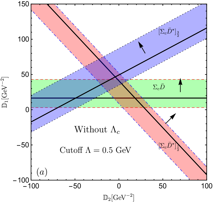
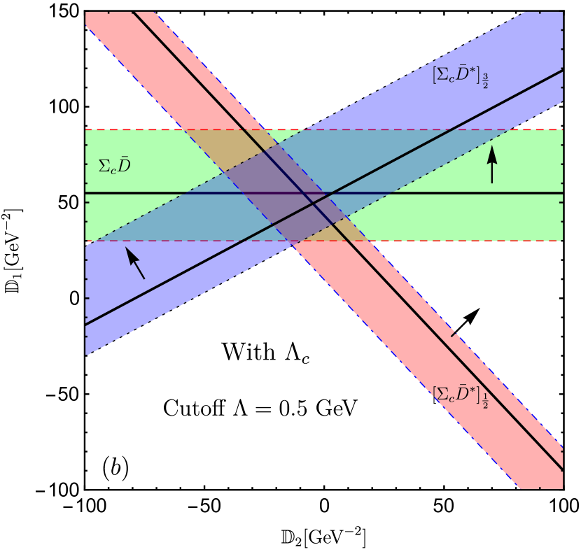
Figure 8: The dependence of the binding energies of the three $P_{c}$ states on the redefined LECs $\mathbb{D}_{1}$ and $\mathbb{D}_{2}$. The green, red and blue bands correspond to the $[\Sigma_{c}\bar{D}]_{J=\frac{1}{2}}$, $[\Sigma_{c}\bar{D}^{\ast}]_{J=\frac{1}{2}}$ and $[\Sigma_{c}\bar{D}^{\ast}]_{J=\frac{3}{2}}$ systems, respectively. The three black straight lines represent the central values of the binding energies obtained from the experimental data Aaij:2019vzc (the numbers in the fifth column of table 1). The boundaries of the bands that are parallel to the corresponding straight lines stand for the regions of parameters with the binding emerges $-30$ MeV and $0$ MeV, respectively. The accompanied arrow shows the direction that the each binding becomes deeper. Figures ($a$) and ($b$) illustrate the results without and with the $\Lambda_{c}$, respectively. The results are both calculated with the cutoff $\Lambda=0.5$ GeV.

The line-shape of the effective potentials for the three $P_{c}$s in this case have been given in ref. Meng:2019ilv , where a set of parameters $\mathbb{D}_{1}=42$ $\textrm{GeV}^{-2}$ and $\mathbb{D}_{2}=-12.5$ $\textrm{GeV}^{-2}$ in the overlap region are adopted. Here, we use these two values to calculate the binding energies of the $[\Sigma_{c}^{(\ast)}\bar{D}^{(\ast)}]_{J}$ systems, the corresponding results are given in the second row of table 2. From table 2 we see that only the result for the $[\Sigma_{c}\bar{D}^{\ast}]_{\frac{3}{2}}$ system is consistent with the data in table 1. There are large differences for the $[\Sigma_{c}\bar{D}]_{\frac{1}{2}}$ and $[\Sigma_{c}\bar{D}^{\ast}]_{\frac{1}{2}}$ systems. In addition, the $[\Sigma_{c}^{\ast}\bar{D}^{\ast}]_{\frac{1}{2}}$ is very shallowly bound, and no binding solutions are found for other high spin systems. We cannot simulate the three $P_{c}$s simultaneously no matter how we choose the values of $\mathbb{D}_{1}$ and $\mathbb{D}_{2}$ in the overlapped region of figure 8(a).

Table 2: The binding energies $\Delta E$ for the $I=\frac{1}{2}$ hidden-charm $[\Sigma_{c}^{(\ast)}\bar{D}^{(\ast)}]_{J}$ systems in both cases with and without the $\Lambda_{c}$, as well as the case with $J^{P}=\frac{1}{2}^{-}$ for $P_{c}(4457)$ and $\frac{3}{2}^{-}$ for $P_{c}(4440)$. The values of $(\mathbb{D}_{1},\mathbb{D}_{2})$ for the ``Without $\Lambda_{c}$" and ``With $\Lambda_{c}$" cases are chosen to be $(42,-12.5)$ $\textrm{GeV}^{-2}$ and $(52,-4)$ $\textrm{GeV}^{-2}$, respectively. ``I.S." stands for the results when interchanging the spins of $P_{c}(4440)$ and $P_{c}(4457)$, where $(\mathbb{D}_{1},\mathbb{D}_{2})=(58,-31)$ $\textrm{GeV}^{-2}$ in this case. ``$\times$" means no binding solution (in units of MeV).

$\Delta E$	$[\Sigma_{c}\bar{D}]_{\frac{1}{2}}$	$[\Sigma_{c}\bar{D}^{\ast}]_{\frac{1}{2}}$	$[\Sigma_{c}\bar{D}^{\ast}]_{\frac{3}{2}}$	$[\Sigma_{c}^{\ast}\bar{D}]_{\frac{3}{2}}$	$[\Sigma_{c}^{\ast}\bar{D}^{\ast}]_{\frac{1}{2}}$	$[\Sigma_{c}^{\ast}\bar{D}^{\ast}]_{\frac{3}{2}}$	$[\Sigma_{c}^{\ast}\bar{D}^{\ast}]_{\frac{5}{2}}$
Without $\Lambda_{c}$	$-29.05$	$-6.84$	$-2.98$	$-34.30$	$-0.16$	$\times$	$\times$
With $\Lambda_{c}$	$-4.60$	$-22.48$	$-3.19$	$-34.51$	$-14.34$	$-3.40$	$-0.30$
I.S.	$-7.24$	$-1.47$	$-17.44$	$-40.88$	$\times$	$-0.24$	$-11.20$

4.2 Role of the $\Lambda_{c}$

As mentioned above, we cannot give a good description for the $P_{c}$s if we only consider the spin partners of $\Sigma_{c}^{(\ast)}$ and $\bar{D}^{(\ast)}$ in the two-pion-exchange diagrams. In this part, we are going to include the contributions of $\Lambda_{c}$ in the loops. Since both the $\Sigma_{c}$ and $\Sigma_{c}^{\ast}$ can decay into $\Lambda_{c}\pi$, the strong couplings between $\Sigma_{c}^{(\ast)}$ and $\Lambda_{c}\pi$ should not be neglected.

The result with the $\Lambda_{c}$ being included is illustrated in figure 8(b), from which we find that there exists a very large overlap among the three colored bands. The small triangle surrounded by three straight lines just locates in the overlap. Besides, the intersection points between two of the three solid lines are very close to each other, and they almost meet at a point if we consider the experimental errors. In other words, the three $P_{c}$ can be synchronously reproduced in this case. The result in figure 8(b) is in good agreement with the experimental data.

We choose the values $\mathbb{D}_{1}=52$ $\textrm{GeV}^{-2}$ and $\mathbb{D}_{2}=-4$ $\textrm{GeV}^{-2}$ in the center of the small triangle to give the binding energies and effective potentials of the $[\Sigma_{c}^{(\ast)}\bar{D}^{(\ast)}]_{J}$ systems. The binding energies in this case are shown in the third row of table 2, from which we get the results for the $[\Sigma_{c}\bar{D}]_{\frac{1}{2}}$, $[\Sigma_{c}\bar{D}^{\ast}]_{\frac{1}{2}}$ and $[\Sigma_{c}\bar{D}^{\ast}]_{\frac{3}{2}}$ systems that are consistent with the experimental data. One may note that the $[\Sigma_{c}^{\ast}\bar{D}]_{\frac{3}{2}}$ system is always deeper bound compared with the other systems regardless of the contribution of $\Lambda_{c}$. The $[\Sigma_{c}^{\ast}\bar{D}]_{\frac{3}{2}}$ system might correspond to the previously reported $P_{c}(4380)$  Aaij:2015tga . Therefore, we urge the experimentalists to reanalyze the data to see whether $P_{c}(4380)$ is the most deeply bound one in the $[\Sigma_{c}^{(\ast)}\bar{D}^{(\ast)}]_{J}$ systems. Moreover, the bound states of the $[\Sigma_{c}^{\ast}\bar{D}^{\ast}]_{J}~{}(J=\frac{1}{2},\frac{3}{2},\frac{5}{2})$ systems are also predicted. Their binding energies are determined to be $-14.34$ MeV, $-3.40$ MeV and $-0.30$ MeV, respectively.

The effective potentials of the $\Sigma_{c}\bar{D}^{(\ast)}$ and $\Sigma_{c}^{\ast}\bar{D}^{(\ast)}$ systems are shown in figures 9 and 10, respectively. In the following, we analyze their behaviors in detail.

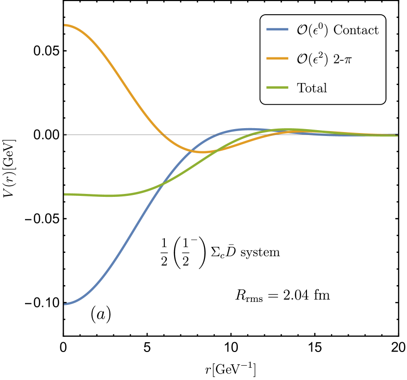
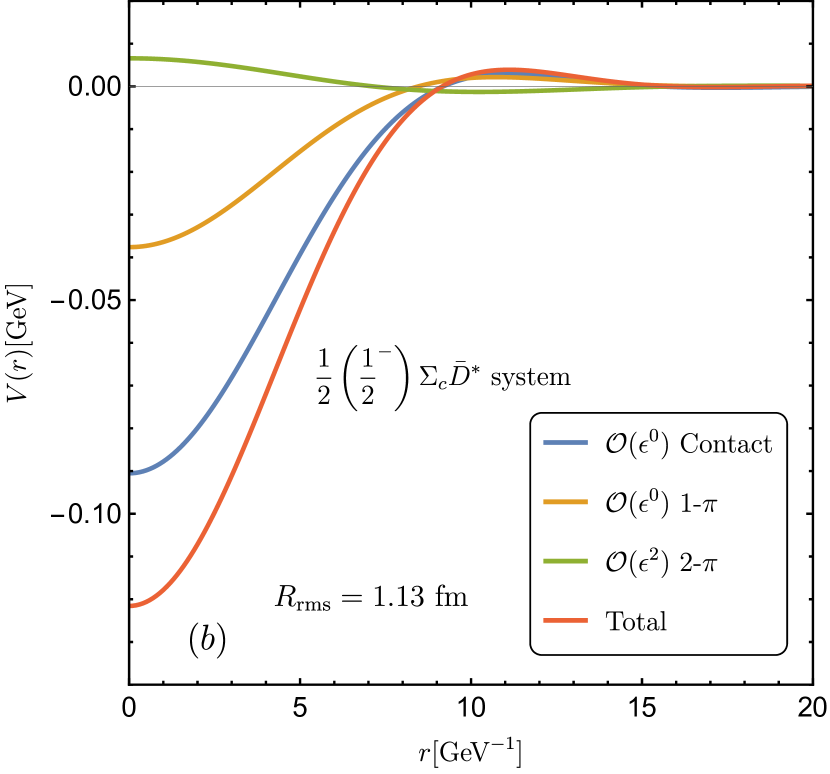
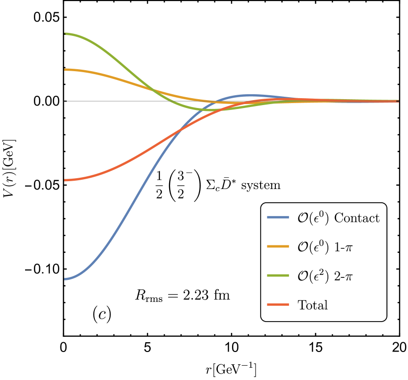
Figure 9: The effective potentials of the $\Sigma_{c}\bar{D}^{(\ast)}$ systems. Their $I(J^{P})$ are marked in each subfigure. The potentials are obtained with the cutoff parameter $\Lambda=0.5$ GeV, and the LECs $\mathbb{D}_{1}=52$ $\textrm{GeV}^{-2}$, $\mathbb{D}_{2}=-4$ $\textrm{GeV}^{-2}$. The $R_{\textrm{rms}}$ in each subfigure denotes the root-mean-square radius of the corresponding system.

$\Sigma_{c}\bar{D}^{(\ast)}$ systems: The results in figures 9(a), 9(b) and 9(c) all demonstrate that the contact term supplies the very strong attractive potential. From eq. (4.1) we know that $\mathcal{O}(\varepsilon^{0})$ contact term for the $\Sigma_{c}\bar{D}$ system only contains the central potential, while the spin-spin contact term appears for the $\Sigma_{c}\bar{D}^{\ast}$ system. Thus their difference is mainly caused by the spin-spin interaction. Meanwhile, the small difference between their $\mathcal{O}(\varepsilon^{0})$ contact potentials indicates that the spin-spin interaction is rather weak and only serves as the hyperfine splittings.

There is no one-pion-exchange potential for the $\Sigma_{c}\bar{D}$ due to the vanishing $\bar{D}\bar{D}\pi$ vertex. The one-pion-exchange potential for the $[\Sigma_{c}\bar{D}^{\ast}]_{\frac{1}{2}}$ is attractive, while it is repulsive for the $[\Sigma_{c}\bar{D}^{\ast}]_{\frac{3}{2}}$ because of the different signs of the matrix element of the spin-spin operator for the spin-$1\over 2$ and spin-$3\over 2$ states.

The contributions of the two-pion-exchange potentials for the $[\Sigma_{c}\bar{D}]_{\frac{1}{2}}$ and $[\Sigma_{c}\bar{D}^{\ast}]_{\frac{3}{2}}$ are significant, but it is marginal for the $[\Sigma_{c}\bar{D}^{\ast}]_{\frac{1}{2}}$. Nevertheless, one can still find the similar behaviours of the two-pion-exchange potentials, which are repulsive at the short range, but become weakly attractive at the intermediate range. This is the typical feature of the nuclear force Machleidt:2011zz .

Finally, the total potentials of the $[\Sigma_{c}\bar{D}^{(\ast)}]_{J}$ systems are fully attractive. The subtle interplay among the short-, intermediate- and long-range interactions yields the experimentally observed $P_{c}(4312)$, $P_{c}(4440)$ and $P_{c}(4457)$.

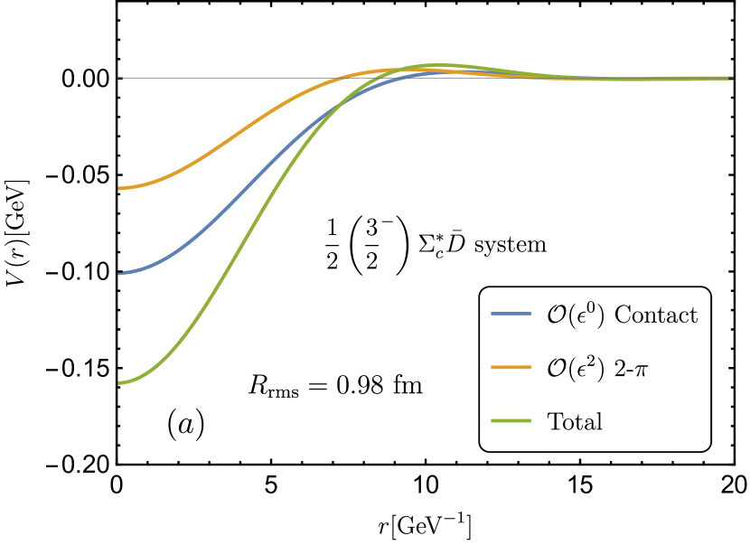
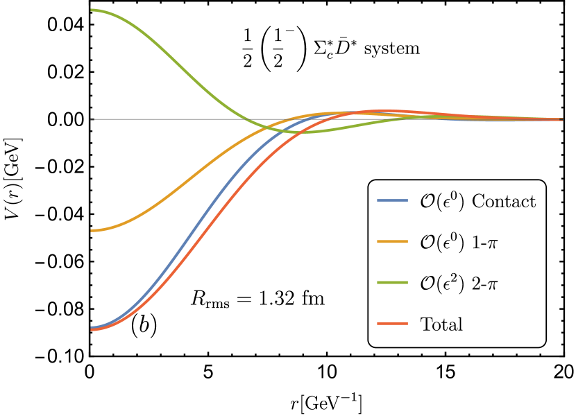
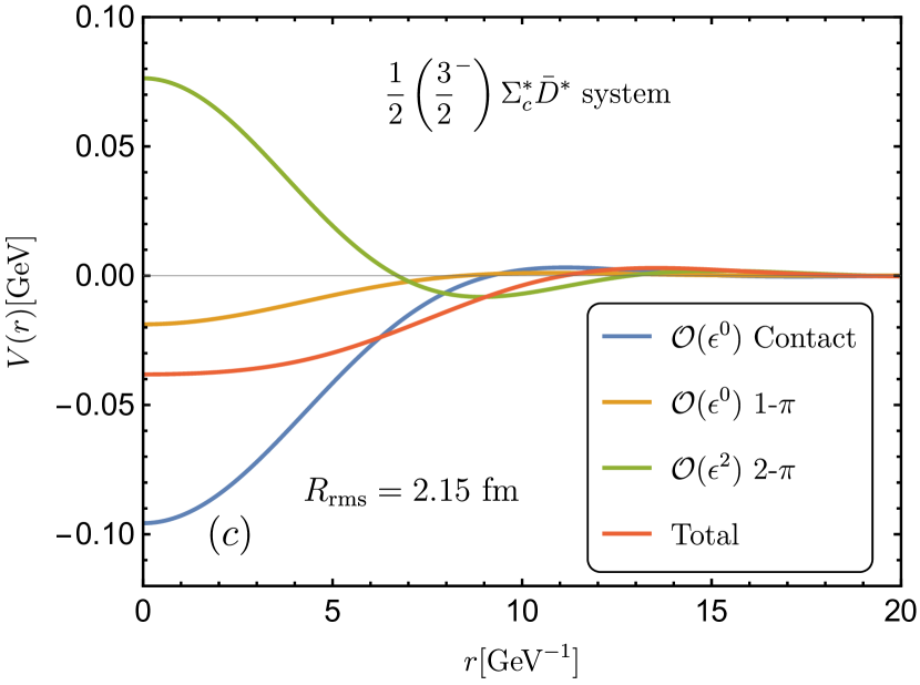
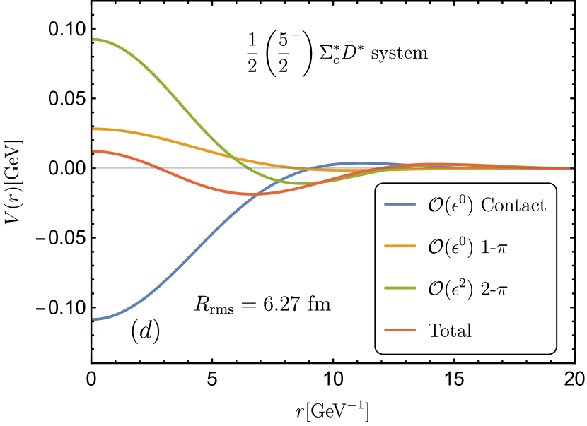
Figure 10: The effective potentials of the $\Sigma_{c}^{\ast}\bar{D}^{(\ast)}$ systems. Their $I(J^{P})$ are marked in each subfigure. The potentials are obtained with the cutoff parameter $\Lambda=0.5$ GeV, and the LECs $\mathbb{D}_{1}=52$ $\textrm{GeV}^{-2}$, $\mathbb{D}_{2}=-4$ $\textrm{GeV}^{-2}$. The $R_{\textrm{rms}}$ in each subfigure denotes the root-mean-square radius of the corresponding system.

$\Sigma_{c}^{(\ast)}\bar{D}^{\ast}$ systems: The results in the figure 10 are also very interesting, since they are related with the previously reported $P_{c}(4380)$ and other unobserved states. Recalling the binding energies in table 2, the result of $\Sigma_{c}^{\ast}\bar{D}$ is about eight times larger than that of the $\Sigma_{c}\bar{D}$. These two systems have the same $\mathcal{O}(\varepsilon^{0})$ contact potentials [e.g., see eq. (4.1)]. The one-pion-exchange contribution vanishes for both systems. Thus the difference can only arise from the two-pion-exchange potentials, as shown in figure 10(a). One can notice the behaviors of the two-pion-exchange potential for the $\Sigma_{c}^{\ast}\bar{D}$ is attractive at the short-range and weakly repulsive at the intermediate-range, which is in contrast to that of the $\Sigma_{c}\bar{D}$ [e.g., see figure 9(a)]. Therefore, if one only considers the $\mathcal{O}(\varepsilon^{0})$ contribution, it is unlikely to obtain the significant difference between the $\Sigma_{c}\bar{D}$ and $\Sigma_{c}^{\ast}\bar{D}$ systems. So we eagerly hope the future analysis at LHCb can help us confirm this observation.

The effective potentials of the $[\Sigma_{c}^{\ast}\bar{D}^{\ast}]_{J}$ systems are very similar to those of the $[\Sigma_{c}\bar{D}^{\ast}]_{J}$ systems. For instance, the $\mathcal{O}(\varepsilon^{0})$ contact potentials are attractive. The one-pion-exchange potentials vary dramatically with the total spins. The two-pion-exchange potentials have the similar line-shape as the nuclear force. Although the total potentials are all attractive, the $[\Sigma_{c}^{\ast}\bar{D}^{\ast}]_{\frac{5}{2}}$ system is very shallowly bound with root-mean-square radius $6.27$ fm.

The two-pion-exchange potentials for the $\Sigma_{c}\bar{D}^{(\ast)}$ systems in different cases are displayed in figure 11. We can read the significant differences when we include the $\Lambda_{c}$ and not, or vary the mass splitting $\delta_{c}$ for the $[\Sigma_{c}\bar{D}]_{\frac{1}{2}}$ and $[\Sigma_{c}\bar{D}^{\ast}]_{\frac{1}{2}}$ systems. We take the $[\Sigma_{c}\bar{D}]_{\frac{1}{2}}$ system as an example. The two-pion-exchange potential is attractive if we do not consider the $\Lambda_{c}$, while it becomes repulsive when the $\Lambda_{c}$ is involved. This can well explain why the binding of the $[\Sigma_{c}\bar{D}]_{\frac{1}{2}}$ state is much deeper without the $\Lambda_{c}$ (see table 2). The magnitude of the change from the minimum to the maximum in these two cases is about $120$ MeV, which is even larger than the minimum of the total potential [see figure 9(a)]. The enhancement is mainly generated by the accidental degeneration of the $\Sigma_{c}\bar{D}$ and $\Lambda_{c}\bar{D}^{\ast}$ systems, since the contribution of the box diagram $(B_{1.1})$ is proportional to $1/(\delta_{c}-\delta_{b})$, where $\delta_{c}-\delta_{b}\simeq 28$ MeV is tiny. Another reason that may cause the enhancement is the contributing diagrams with the $\Lambda_{c}$ are only $(T_{1.3})$ and $(B_{1.1})$. Unlike the $\Sigma_{c}\bar{D}^{\ast}$ system, the accidental cancelations among several diagrams cannot happen. In other words, the $\Lambda_{c}$ indeed plays a crucial role in the formation of the $P_{c}(4312)$.

For the $[\Sigma_{c}\bar{D}^{\ast}]_{\frac{1}{2}}$ system, since the whole contribution of the two-pion-exchange potential is much weaker than the $\mathcal{O}(\varepsilon^{0})$ contact term [see figure 9(b)], the influence of $\Lambda_{c}$ on this state is not so apparent as in $\Sigma_{c}\bar{D}$. However, it is still very important to the existence of $P_{c}(4457)$ and the possible $[\Sigma_{c}^{\ast}\bar{D}^{\ast}]_{J}$ bound states (e.g., see the data in table 2).

In figure 11, we also show the dependence of the two-pion-exchange potentials on the mass splitting $\delta_{c}$. One can see that they are very sensitive to the $\delta_{c}$. The loop integrals generally contain two structures. One is the analytic term, which is the polynomials of the $m_{\pi}^{2}$, $\bm{q}^{2}$, $\delta^{2}$, etc.. Another one is the nonanalytic term, which comprises the typical multivalued functions, such as $\log\mathcal{X}$ and $\sqrt{\mathcal{X}}$ ($\mathcal{X}$ is the polynomials of the $m_{\pi}^{2}$, $\bm{q}^{2}$, $\delta^{2}$.). The physical value of the $\delta_{c}$ is about $168$ MeV, which is larger than the pion mass $m_{\pi}$. We then decrease its value to $100$ MeV and $65$ MeV. One can anticipate the dependence on $\delta$ is regular if the terms that make up the potential are only polynomials, but the variation trend in figure 11 is irregular. This phenomenon indicates the nonanalytic terms can distort the $\mathcal{O}(\varepsilon^{2})$ potentials, which are vital to the formations of the $P_{c}$ states. The contributions of the nonanalytic terms incorporate the complicated light quark dynamics, which are almost impossible to estimate from quark models.

After the above discussions, one may wonder whether it is possible to reproduce the three $P_{c}$s simultaneously if we only consider the contribution of the $\Lambda_{c}$. The result in this case is given in figure 12(a), which is also unsatisfactory as in the case of figure 8(a). Therefore, both the $\Lambda_{c}$ and the spin partners of the $\Sigma_{c}^{(\ast)}$ and $\bar{D}^{(\ast)}$ are indispensable. Their subtle interaction leads to the synchronous emergence of the $P_{c}(4312)$, $P_{c}(4440)$ and $P_{c}(4457)$.

The complete mass spectra of the hidden-charm molecular pentaquarks are shown in figure 13(a). We see that the $P_{c}(4312)$, $P_{c}(4440)$ and $P_{c}(4457)$ can be well interpreted as the $[\Sigma_{c}\bar{D}]_{\frac{1}{2}}$, $[\Sigma_{c}\bar{D}^{\ast}]_{\frac{1}{2}}$ and $[\Sigma_{c}\bar{D}^{\ast}]_{\frac{3}{2}}$ molecules. $P_{c}(4380)$ might be the deeper bound $[\Sigma_{c}^{\ast}\bar{D}]_{\frac{3}{2}}$ molecules. There are also other possible $P_{c}$s composed of the $[\Sigma_{c}^{\ast}\bar{D}^{\ast}]_{J}$. Future search for these states at LHCb is very important for establishing a complete family of the hidden-charm pentaquarks.

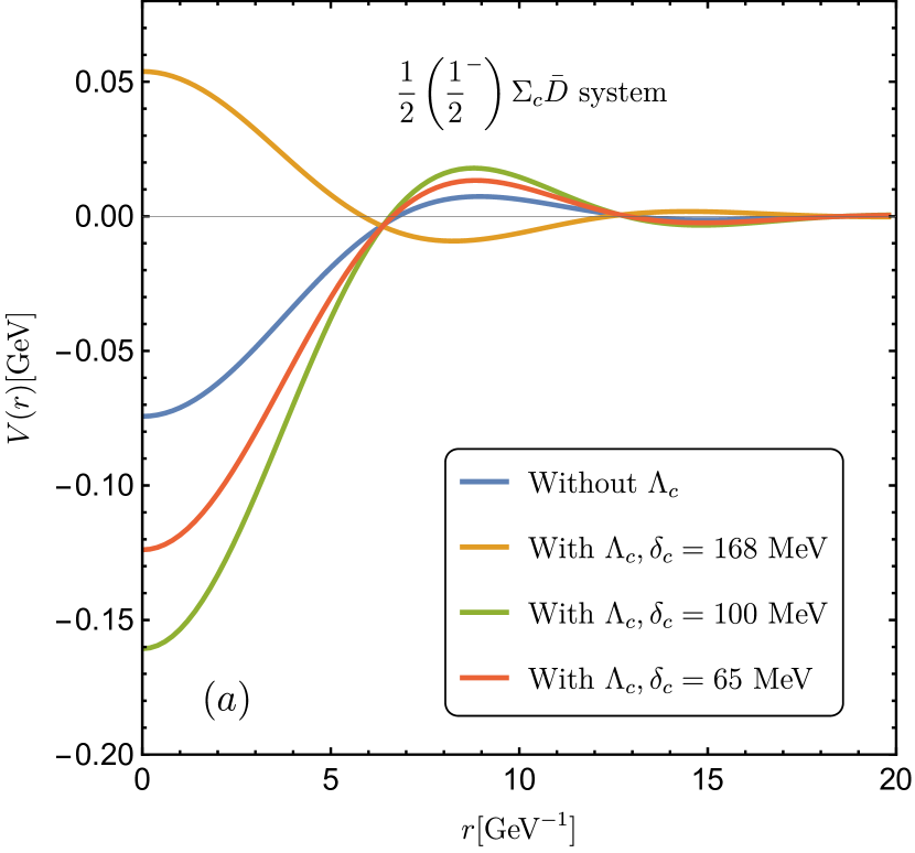
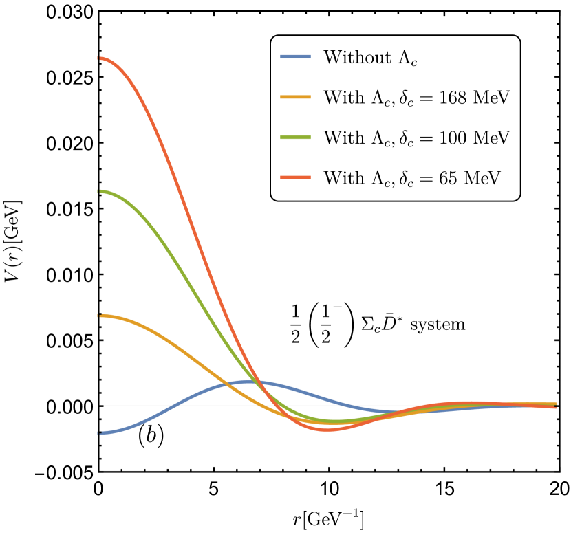
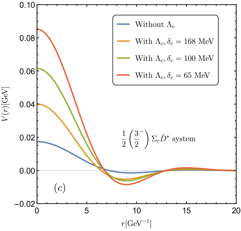
Figure 11: The variations of the two-pion-exchange potentials for the $\Sigma_{c}\bar{D}^{(\ast)}$ systems in the cases of without and with the $\Lambda_{c}$. Their $I(J^{P})$ are marked in each subfigure. The dependence on the mass splitting $\delta_{c}$ is also illustrated.

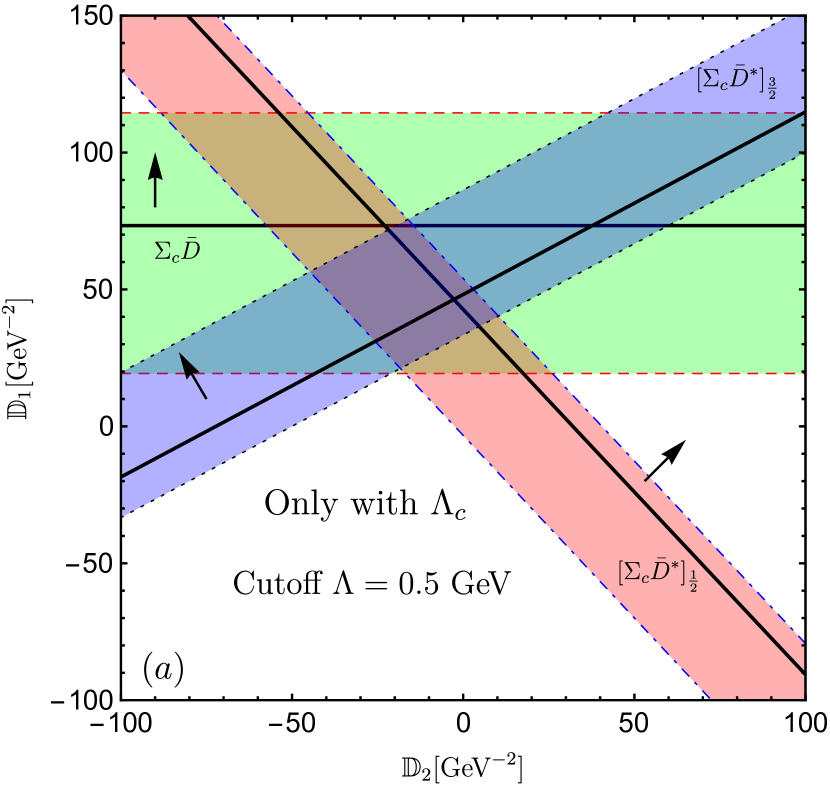
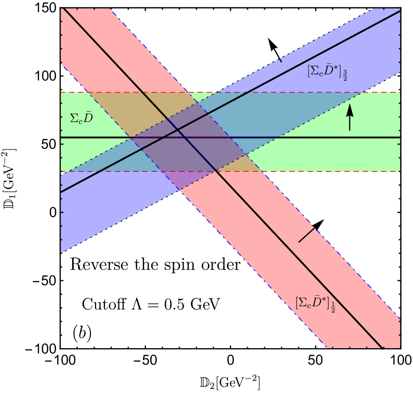
Figure 12: The dependence of the binding energies of the three $P_{c}$ states on the redefined LECs $\mathbb{D}_{1}$ and $\mathbb{D}_{2}$ in different cases. Figure ($a$) gives the result that only considering the contributions of $\Lambda_{c}$ in the two-pion-exchange diagrams. Figure ($b$) shows the result when interchanging the spins of $P_{c}(4440)$ and $P_{c}(4457)$. The notations are the same as those in figure 8.

4.3 An episode: interchanging the spins of $P_{c}(4440)$ and $P_{c}(4457)$

The $J^{P}$ quantum numbers of the $P_{c}(4312)$, $P_{c}(4440)$ and $P_{c}(4457)$ are not determined yet Aaij:2019vzc . The theoretically favored $J^{P}$ for $P_{c}(4440)$ and $P_{c}(4457)$ in this paper and some previous works Meng:2019ilv ; Liu:2019tjn ; Chen:2019asm ; Xiao:2019aya ; He:2019ify are $\frac{1}{2}^{-}$ and $\frac{3}{2}^{-}$, respectively. Nevertheless, in some recent works Yamaguchi:2019seo ; Valderrama:2019chc ; Liu:2019zvb , a new conjecture, that the $J^{P}=\frac{3}{2}^{-}$ for $P_{c}(4440)$ and $\frac{1}{2}^{-}$ for $P_{c}(4457)$, is proposed. In this subsection, we investigate the possibility of this spin assignment.

The result of interchanging the spin assignment of $P_{c}(4440)$ and $P_{c}(4457)$ is given in figure 12(b). Marvelously, the result is comparable with the one in figure 8(b), i.e., it seems this assignment can well describe the experimental data, likewise. However, one shall note that the values of the LECs $(\mathbb{D}_{1},\mathbb{D}_{2})$ in the center of the small triangle are $(58,-31)$ $\textrm{GeV}^{-2}$, while these values in figure 8(b) are $(52,-4)$ $\textrm{GeV}^{-2}$. The shift of $\mathbb{D}_{1}$ in these two cases is small, but the $\mathbb{D}_{2}$ in the first case is about eight times larger than that of the latter one. One has to largely enhance the contribution of the $\mathcal{O}(\varepsilon^{0})$ spin-spin interaction to reverse the canonical order of the spins of $P_{c}(4440)$ and $P_{c}(4457)$.

The binding energies of the $[\Sigma_{c}^{(\ast)}\bar{D}^{(\ast)}]_{J}$ systems with the $(\mathbb{D}_{1},\mathbb{D}_{2})=(58,-31)$ $\textrm{GeV}^{-2}$ are listed in the fourth row of table 2. Although the binding energies of the $[\Sigma_{c}\bar{D}]_{\frac{1}{2}}$, $[\Sigma_{c}\bar{D}^{\ast}]_{\frac{1}{2}}$ and $[\Sigma_{c}\bar{D}^{\ast}]_{\frac{3}{2}}$ can match the ones of $P_{c}(4312)$, $P_{c}(4457)$ and $P_{c}(4440)$, other predictions are different from those with the previous spin assignment. The bound $[\Sigma_{c}^{\ast}\bar{D}^{\ast}]_{\frac{1}{2}}$ state does not exist, the $[\Sigma_{c}^{\ast}\bar{D}^{\ast}]_{\frac{3}{2}}$ state is very shallowly bound, and the binding of the $[\Sigma_{c}^{\ast}\bar{D}^{\ast}]_{\frac{5}{2}}$ state is much deeper. This result is very theatrical to some extent, since the lowest spin state of the $\Sigma_{c}^{\ast}\bar{D}^{\ast}$ does not exist. However, this phenomenon does not occur in the leading order effective field theory where there does not exist the repulsive core from the two-pion-exchange diagrams.

The information from figure 8(b) indicates the $\mathbb{D}_{1}$ and $\mathbb{D}_{2}$ always have the opposite sign, and the ratio of their absolute values $\mathcal{R}_{12}=|\mathbb{D}_{1}|/|\mathbb{D}_{2}|\simeq 13$. We notice the correspondence and consistence with the $N$-$N$ system. The leading order contact Lagrangian for the $N$-$N$ system reads Machleidt:2011zz ,

$$\mathcal{L}_{NN}^{(0)}=-\frac{1}{2}C_{S}(\bar{N}N)(\bar{N}N)-\frac{1}{2}C_{T}(\bar{N}\bm{\sigma}N)\cdot(\bar{N}\bm{\sigma}N),$$ (84)

where $C_{S}$ and $C_{T}$ are two independent LECs. One would see that they respectively correspond to the $\mathbb{D}_{1}$ and $\mathbb{D}_{2}$ in our work if we write out the $\mathcal{O}(\varepsilon^{0})$ contact potential of the $N$-$N$ system,

$$\mathcal{V}_{NN}=C_{S}+C_{T}\bm{\sigma}\cdot\bm{\sigma}.$$ (85)

The values of $C_{S}$ and $C_{T}$ have been precisely determined by fitting the $np$ scattering phase shift at the next-to-next-to-next-to-leading order of chiral perturbation theory Entem:2003ft . For the $np$ system, which gives

$$C_{S}=-100.28~{}\textrm{GeV}^{-2},\qquad C_{T}=5.61~{}\textrm{GeV}^{-2}.$$ (86)

If absorbing the minus sign of eq. (84) into the $C_{S}$ and $C_{T}$, one would see the redefined $C_{S}$ and $C_{T}$ share the same sign with the $\mathbb{D}_{1}$ and $\mathbb{D}_{2}$, correspondingly. Meanwhile, the ratio of the absolute values for $C_{S}$ and $C_{T}$ gives $\mathcal{R}_{ST}=|C_{S}|/|C_{T}|\simeq 18$, which is compatible with the $\mathcal{R}_{12}$ for $\mathbb{D}_{1}$ and $\mathbb{D}_{2}$. However, this ratio for the case of interchanging the spins of $P_{c}(4440)$ and $P_{c}(4457)$ is about $1.9$, which is one order of magnitude smaller than the $\mathcal{R}_{ST}$, because of the spin-spin term in the contact potential is immoderately enhanced.

On the one hand, from the point of potential model, the spin-spin term is suppressed by the factor $1/(m_{\Sigma_{c}^{(\ast)}}m_{D^{(\ast)}})$ (e.g., see appendix D). On the other hand, one can build a mandatory connection between the contact terms of chiral effective field theory and the one-boson-exchange model with the help of resonance saturation model Epelbaum:2001fm ; Ecker:1988te . As the heavy fields, $\rho$, $\omega$, $f_{0}$, $a_{0}$, etc., which are equally treated in one-boson-exchange model, are integrated out in chiral effective field theory, and their contributions are packaged into the LECs. The $(\omega,f_{0})$ and $(\rho,a_{0})$ mesons account for the isospin-isospin unrelated $D_{a}$ and related $E_{a}$, respectively [e.g., see eq. (22)] Xu:2017tsr . Meanwhile, the $\omega$ and $\rho$ mesons couple to the matter fields via the $P$-wave interaction due to the parity conservation. Each vertex contains one momentum. In other words, the $\omega$ and $\rho$ mesons are responsible for the momentum-dependent spin-spin interaction, which cannot be matched with the $\mathcal{O}(\varepsilon^{0})$ $D_{b}$ and $E_{b}$. Therefore, the momentum-independent contributions for $D_{b}$ and $E_{b}$ can only come from the axial-vector mesons, such as $(h_{1},f_{1})$ and $(b_{1},a_{1})$. The masses of these states reside around $1.2$ GeV, which are much heavier than those of $\omega$ and $\rho$, and suppress the value of $\mathbb{D}_{2}$.

5 Hidden-bottom molecular pentaquarks

The above study for the hidden-charm pentaquarks can be extended to the hidden-bottom case, once the coupling constants and mass splittings are replaced by the bottomed ones. The coupling constants $g_{2}$ and $g_{4}$ for the bottom baryons can be calculated with the partial decay widths of $\Sigma_{b}\to\Lambda_{b}\pi$ and $\Sigma_{b}^{\ast}\to\Lambda_{b}\pi$ Tanabashi:2018oca ,

$$\Gamma(\Sigma_{b}\to\Lambda_{b}\pi) = \frac{g_{2}^{2}}{4\pi f_{\pi}^{2}}\frac{m_{\Lambda_{b}}}{m_{\Sigma_{b}}}|\bm{q}_{\pi}|^{3},\qquad\qquad\Gamma(\Sigma_{b}^{\ast}\to\Lambda_{b}\pi)=\frac{g_{4}^{2}}{12\pi f_{\pi}^{2}}\frac{m_{\Lambda_{b}}}{m_{\Sigma_{b}^{\ast}}}|\bm{q}_{\pi}|^{3},$$ (87)

Using the average values of the decay widths of $\Sigma_{b}^{+}\to\Lambda_{b}^{0}\pi^{+}$ and $\Sigma_{b}^{\ast+}\to\Lambda_{b}^{0}\pi^{+}$ Tanabashi:2018oca , we get $g_{2}=-0.51$, $g_{4}=0.91$. The other couplings can then be obtained with the relations in eq. (2.1), which yield,

$$g_{1}=0.83,\qquad g_{3}=0.72,\qquad g_{5}=-1.25.$$ (88)

The axial coupling $g$ of the $B$ mesons cannot be directly derived from the experiments due to absence of phase space for $B^{\ast}\to B\pi$, so we adopt the average value $g=-0.52$ from the lattice calculations Ohki:2008py ; Detmold:2012ge . Similarly, the mass splittings are correspondingly given by

$$\delta_{a} =m_{\Sigma_{b}^{\ast}}-m_{\Sigma_{b}}\simeq 20~{}\textrm{MeV}, \delta_{b} =m_{B^{\ast}}-m_{B}\simeq 45~{}\textrm{MeV},$$

$$\delta_{c} =m_{\Sigma_{b}}-m_{\Lambda_{b}}\simeq 191~{}\textrm{MeV}, \delta_{d} =m_{\Sigma_{b}^{\ast}}-m_{\Lambda_{b}}\simeq 211~{}\textrm{MeV},$$ (89)

where the masses of the $\Sigma_{b}^{(\ast)+}$ and $B^{(\ast)0}$ are used Tanabashi:2018oca .

The small scale expansion Hemmert:1997ye is used in eqs. (16) and (20), i.e., the mass splitting $\delta$ is treated as another small scale in the Lagrangians. This expansion works well for the systems with one heavy matter field Wang:2019mhm . The loop integrals in these systems are the polynomials of $\delta$, thus the convergence of the chiral expansion is not affected as long as the $\delta\sim m_{\pi}$ or smaller than $m_{\pi}$. But the situation becomes different for the systems with two heavy matter fields. The loop integral of the box diagram is proportional to $1/(\delta_{x}+\delta_{y})$. If $\delta_{x}+\delta_{y}$ is of the order of the pion mass, the convergence of the expansion could still be good. For example, for the $\Sigma_{c}^{(\ast)}\bar{D}^{(\ast)}$ systems Meng:2019ilv , $\delta_{b}-\delta_{a}\simeq 80$ MeV. However, for the $\Sigma_{b}^{(\ast)}B^{(\ast)}$ systems, $\delta_{b}-\delta_{a}\simeq 25$ MeV, which is much smaller that the pion mass. Therefore, if we still adopt the same procedure as used in the $\Sigma_{c}^{(\ast)}\bar{D}^{(\ast)}$ systems, the amplitudes of some typical box diagrams would be largely amplified, which results in extremely strong attractive or repulsive potential. This is unphysical and mainly caused by the poles of the heavy matter fields. In some previous works Meng:2019ilv ; Wang:2018atz , the mass splittings are discarded in the box diagrams to subtract the 2PR contributions. Here, we develop a method to remove the heavy matter field poles in the box diagrams with the mass splittings being kept (see appendix B for more details).

In order to predict the possible $P_{b}$ states, we also need to know the LECs $\mathbb{D}_{1}$ and $\mathbb{D}_{2}$ for the $\Sigma_{b}^{(\ast)}B^{(\ast)}$ systems. In principle, they should be fixed from experimental data or the results from lattice QCD, which are not available at present. Thus, we estimate the ranges of $\mathbb{D}_{1}$ and $\mathbb{D}_{2}$. Generally, the values of $\mathbb{D}_{1}$ and $\mathbb{D}_{2}$ are different for the $\Sigma_{b}^{(\ast)}B^{(\ast)}$ and $\Sigma_{c}^{(\ast)}\bar{D}^{(\ast)}$ systems. One explicit example is that the axial coupling constants for the bottom sectors are about $17\%$ smaller than those of the charmed sectors. Therefore, we take the values $(\mathbb{D}_{1},\mathbb{D}_{2})=(52,-4)$ GeV^-2 fixed for the $P_{c}$s with at most $17\%$ deviation to give the ranges of $\mathbb{D}_{1}$ and $\mathbb{D}_{2}$ in the hidden-bottom case.

We set the $(52,-4)$ GeV^-2 as the limits of $(\mathbb{D}_{1},\mathbb{D}_{2})$ for the bottom case, which deviate $17\%$ from the central value. Approximately, we have

$$\mathbb{D}_{1}=43\pm 9~{}\textrm{GeV}^{-2},\qquad\mathbb{D}_{2}=-3.3\mp 0.7~{}\textrm{GeV}^{-2}.$$ (90)

The binding energies and the mass spectra are given in table 3 and figure 13(b), respectively. We notice the hidden-bottom ones are the tightly bound molecules due to the large masses of their components. Unlike the $[\Sigma_{c}^{\ast}\bar{D}^{\ast}]_{J}$ systems, the gaps between the thresholds of the $[\Sigma_{b}^{\ast}B^{\ast}]_{J}$ systems are only about $20$ MeV. Thus the masses of some peculiar states with binding energies $\Delta E<-20$ MeV may not only lie below its corresponding threshold but also the lower one. For example, the molecular state $[\Sigma_{b}^{\ast}B^{\ast}]_{\frac{1}{2}}$ locates below the thresholds of $\Sigma_{b}B^{\ast}$ and $\Sigma_{b}^{\ast}B^{\ast}$ if we only consider the central value.

The masses of the hidden-bottom molecules are all above $11$ GeV. Like their $P_{c}$ partners, they may be observed from the $\Upsilon(1S)N$ and $\Upsilon(2S)N$ final states. We hope future experiments to hunt for these $P_{b}$ states. We conclude this section by borrowing one of the famous phrases from R. P. Feynman: ``There is plenty of room at the `bottom'." Feynman:1959rpf

Table 3: The binding energies $\Delta E$ for the $I=\frac{1}{2}$ hidden-bottom $[\Sigma_{b}^{(\ast)}B^{(\ast)}]_{J}$ systems with the contribution of the $\Lambda_{b}$. The values of $(\mathbb{D}_{1},\mathbb{D}_{2})$ are chosen to be $(43\pm 9,-3.3\mp 0.7)$ $\textrm{GeV}^{-2}$, the cutoff $\Lambda=0.5$ GeV (in units of MeV).

$\Delta E$	$[\Sigma_{b}B]_{\frac{1}{2}}$	$[\Sigma_{b}B^{\ast}]_{\frac{1}{2}}$	$[\Sigma_{b}B^{\ast}]_{\frac{3}{2}}$	$[\Sigma_{b}^{\ast}B]_{\frac{3}{2}}$	$[\Sigma_{b}^{\ast}B^{\ast}]_{\frac{1}{2}}$	$[\Sigma_{b}^{\ast}B^{\ast}]_{\frac{3}{2}}$	$[\Sigma_{b}^{\ast}B^{\ast}]_{\frac{5}{2}}$
With $\Lambda_{b}$	$-14.04^{+7.36}_{-8.92}$	$-22.72^{+8.03}_{-9.34}$	$-9.12^{+6.06}_{-8.34}$	$-14.74^{+7.54}_{-9.05}$	$-25.75^{+8.38}_{-9.06}$	$-17.76^{+7.91}_{-9.07}$	$-7.81^{+5.56}_{-8.41}$

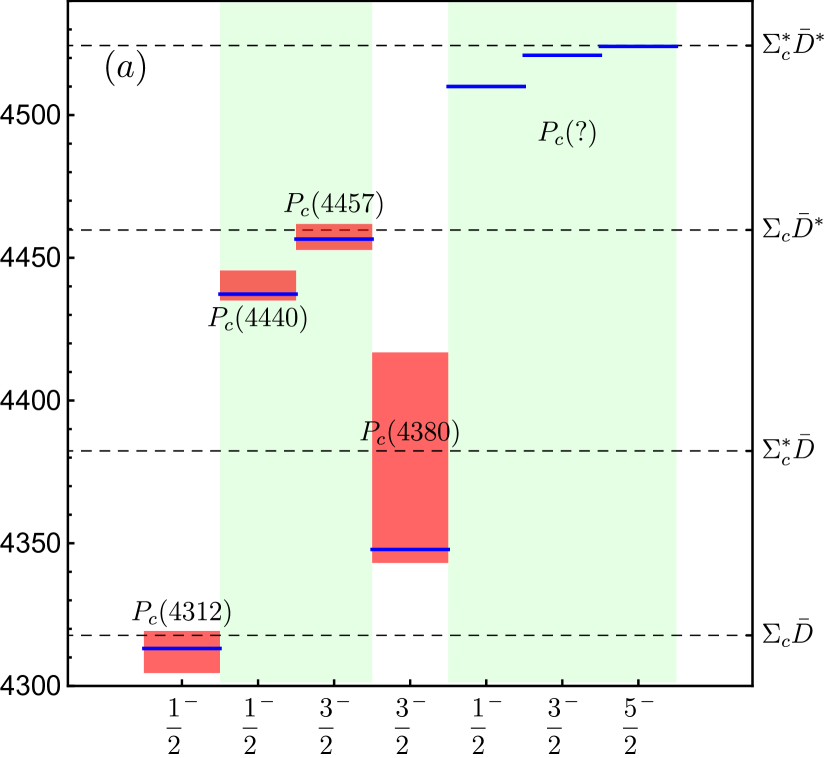
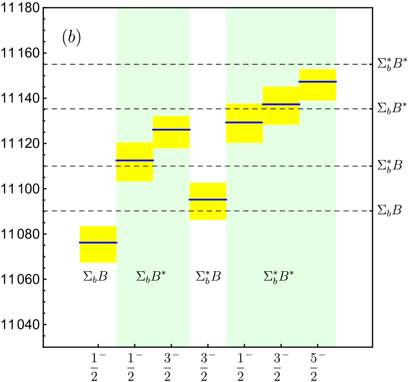
Figure 13: The mass spectra of the hidden-charm ($a$) and hidden-bottom ($b$) molecular pentaquarks. The red and yellow regions in figures ($a$) and ($b$) denote the mass ranges obtained from the experimental measurements and theoretical estimations, respectively. The blue solid lines represent the central values in our calculations. The black dashed lines are the corresponding thresholds.

6 Heavy quark symmetry breaking effect

The QCD Lagrangian has heavy quark symmetry (HQS) when the heavy quark mass $m_{Q}\to\infty$. For a heavy hadron containing one single heavy quark, the strong interaction would be independent of the heavy flavors in this limit. Meanwhile, the heavy quark will decouple with the light degrees of freedom. The multiplet associated with the heavy quark spin would be degenerate in the heavy quark limit. However, the physical masses of the heavy quarks are finite, such as $m_{c}\sim 1.5$ GeV, $m_{b}\sim 5$ GeV. Therefore, the effects of the heavy quark flavor symmetry breaking and spin symmetry breaking are explicit. For example, the axial coupling $g$ for $B^{\ast}B\pi$ is about $17\%$ smaller that that of the $D^{\ast}D\pi$. Thus the value $17\%$ can be roughly regarded as the breaking size of the heavy quark flavor symmetry. In addition, the heavy quark spin symmetry (HQSS) breaking is more obvious, such as the mass splittings of $(B^{\ast},B)$ and $(D^{\ast},D)$ are about $45$ MeV and $142$ MeV, respectively.

HQS can be used to relate the coupling constants to one another, such as the axial coupling constants in the $\mathcal{O}(\varepsilon^{0})$ Lagrangians. Under HQS, the heavy quarks only serve as the spectators. The interaction between $\Sigma_{c}^{(\ast)}$ and $\bar{D}^{(\ast)}$ is mediated by their inner light degrees of freedom, i.e., the light diquarks in $\Sigma_{c}^{(\ast)}$ and the light quark in $\bar{D}^{(\ast)}$. Therefore, the $S$-wave effective potentials between $\Sigma_{c}^{(\ast)}$ and $\bar{D}^{(\ast)}$ at the quark level can be parameterized as Meng:2019ilv

$$V^{\mathrm{HQS}}_{\mathrm{quark-level}}=V_{c}+V_{s}\bm{l}_{1}\cdot\bm{l}_{2},$$ (91)

where $V_{c}$ and $V_{s}$ denote the central term and spin-spin term, respectively. $\bm{l}_{1}$ and $\bm{l}_{2}$ are the spins of the light degrees of freedom of the $\Sigma_{c}^{(\ast)}$ and $\bar{D}^{(\ast)}$, respectively. With the potentials at the quark level, one can build the relations between different channels at the hadron level by parameterizing the hadron level potentials as

$$\mathcal{V}_{\Sigma_{c}\bar{D}} = \mathcal{V}_{1},\qquad\mathcal{V}_{\Sigma_{c}\bar{D}^{\ast}}=\mathcal{V}_{2}+\mathcal{V}_{2}^{\prime}\bm{S}_{1}\cdot\bm{S}_{2},$$

$$\mathcal{V}_{\Sigma_{c}^{\ast}\bar{D}} = \mathcal{V}_{3},\qquad\mathcal{V}_{\Sigma_{c}^{\ast}\bar{D}^{\ast}}=\mathcal{V}_{4}+\mathcal{V}_{4}^{\prime}\bm{S}_{1}\cdot\bm{S}_{2},$$ (92)

where $\bm{S}_{1}$ and $\bm{S}_{2}$ are the spin operators of the $\Sigma_{c}^{(\ast)}$ and $\bar{D}^{\ast}$, respectively. One can easily verify

$$\mathcal{V}_{1}=\mathcal{V}_{2}=\mathcal{V}_{3}=\mathcal{V}_{4}=V_{c};\qquad\mathcal{V}_{2}^{\prime}=\frac{2}{3}V_{s},\quad\mathcal{V}_{4}^{\prime}=\frac{1}{3}V_{s}.$$ (93)

The leading order potentials obviously satisfy the above relations obtained from HQS. One can also testify the one-loop level analytical expressions satisfy the above relations as well when $d\to 4$ and $\delta_{a,b}\to 0$.

The HQS breaking effect would manifest itself in the loop diagrams if $\delta_{a,b}\neq 0$ . When $\delta_{a}=\delta_{b}=0$, all the box diagrams would become the 2PR ones, thus we have to remove the 2PR contributions. In order to compare with the cases of $\delta_{a}=\delta_{b}=0$, we also subtract the 2PR contributions from the $(\delta_{a},\delta_{b})\neq 0$ cases (see appendix B). The 2PI two-pion-exchange potentials for the $\Sigma_{c}^{(\ast)}\bar{D}^{(\ast)}$ and $\Sigma_{b}^{(\ast)}B^{(\ast)}$ systems with and without HQS are illustrated in figure 14. We notice the HQS keeps relatively good for the $[\Sigma_{c}\bar{D}^{\ast}]_{J}/[\Sigma_{b}B^{\ast}]_{J}$ and $[\Sigma_{c}^{\ast}\bar{D}^{\ast}]_{J}/[\Sigma_{b}^{\ast}B^{\ast}]_{J}$ systems, while it breaks significantly for the $[\Sigma_{c}\bar{D}]_{J}$ and $[\Sigma_{c}^{\ast}\bar{D}]_{J}$ systems. When $\delta_{a}=\delta_{b}=0$, the two-pion-exchange potential of the $[\Sigma_{c}\bar{D}]_{J}$ system is exactly equal to that of the $[\Sigma_{c}^{\ast}\bar{D}]_{J}$ system, which satisfies the relations in eq. (93). However, when we set the physical mas splitting, $(\delta_{a},\delta_{b})=(65,142)$ MeV, the line-shapes are explicitly modified and the relations in eq. (93) are obviously violated. The quantum fluctuation at the loop level would break the HQS significantly. The predictions inherited from HQS should be carefully reexamined, at least for the $[\Sigma_{c}\bar{D}]_{J}$ and $[\Sigma_{c}^{\ast}\bar{D}]_{J}$ systems. Besides, the HQS in the hidden-bottom systems is better than that of the hidden-charm cases as expected.

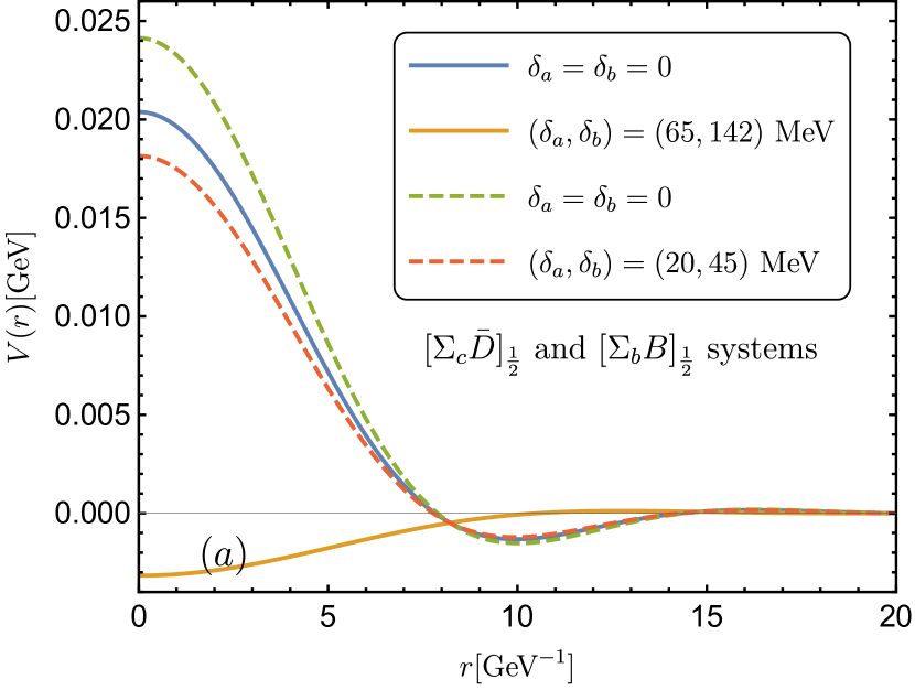
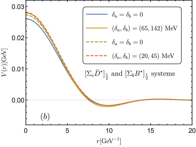
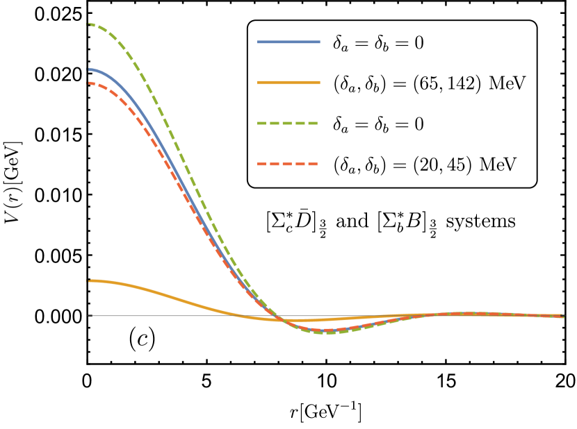
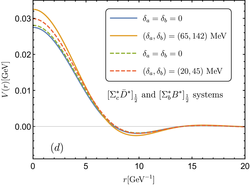
Figure 14: The heavy quark symmetry breaking phenomena in the two-pion-exchange diagrams. The solid lines denote the $\Sigma_{c}^{(\ast)}\bar{D}^{(\ast)}$ systems with vanishing mass splittings and physical mass splittings. The dashed lines represent the same cases but for the $\Sigma_{b}^{(\ast)}B^{(\ast)}$ systems. The unlisted systems share the similar behaviors as their spin partners.

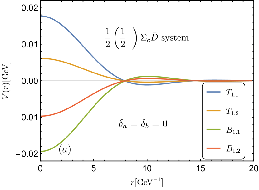
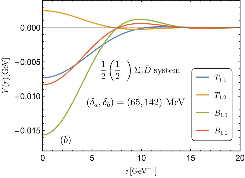
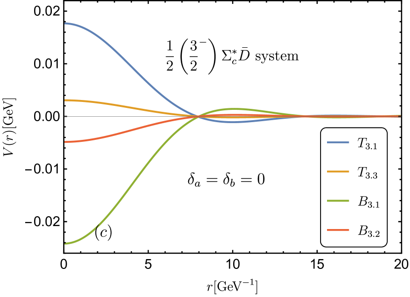
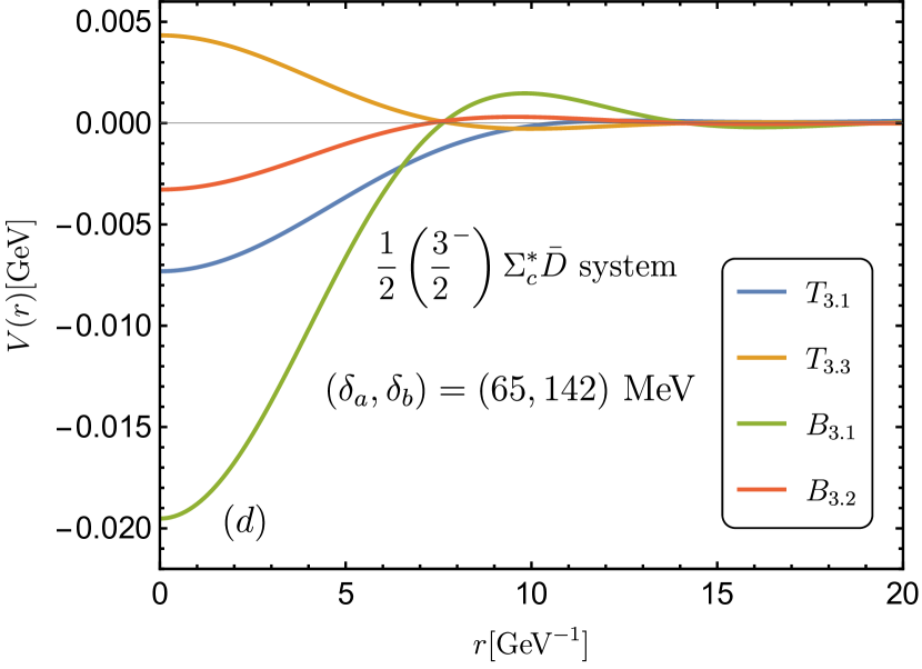
Figure 15: The behaviors of the two-pion-exchange potentials of each mass splitting related 2PI diagrams for the $[\Sigma_{c}\bar{D}]_{\frac{1}{2}}$ [($a$), ($b$)] and $[\Sigma_{c}^{\ast}\bar{D}]_{\frac{3}{2}}$ [($c$), ($d$)] systems in the cases of $\delta_{a}=\delta_{b}=0$ and $(\delta_{a},\delta_{b})=(65,142)$ MeV, respectively.

In the following, we investigate the HQSS violation effect of each Feynman diagram for the $[\Sigma_{c}\bar{D}]_{\frac{1}{2}}$ and $[\Sigma_{c}^{\ast}\bar{D}]_{\frac{3}{2}}$ systems. The results are shown in figure 15. When $\delta_{a}=\delta_{b}=0$, the contributions from the triangle diagrams and box diagrams are always repulsive and attractive, respectively. The differences between the corresponding diagrams, such as $(B_{1.1})$ and $(B_{3.1})$, are mainly caused by the coupling constants. However, when the mass splittings are considered, the magnitudes of most diagrams except for $(T_{1.1})$ and $(T_{3.1})$ would change. The signs of the potentials from $(T_{1.1})$ and $(T_{3.1})$ are changed. The HQSS breaking mainly originates from these two diagrams. The repulsive contributions of the two diagrams in the heavy quark limits become attractive when the mass splittings are included. Inspecting the analytical expressions of the triangle diagrams for the $\Sigma_{c}^{(\ast)}\bar{D}^{(\ast)}$ systems, we would see that

$$\mathcal{V}_{\Sigma_{c}^{(\ast)}\bar{D}^{(\ast)}}^{T_{i.j}}\sim(\mathbf{I}_{1}\cdot\mathbf{I}_{2})\Big{[}AJ_{34}^{T}-B\bm{q}^{2}\left(J_{24}^{T}+J_{33}^{T}\right)\Big{]}(m_{\pi},\omega,q),$$ (94)

where $A$ and $B$ are the positive numbers. The corresponding $J_{ij}^{T}$ functions generally contain two structures, the odd function of $\omega$ and the even one (see appendix A). The odd part is proportional to

$$\omega\int_{0}^{1}dx\mathscr{F}(x,m_{\pi},\omega,\bm{q})+\int_{-\omega}^{0}dy\int_{0}^{1}dx\mathscr{G}(x,y,m_{\pi},\omega,\bm{q}),$$ (95)

where $\mathscr{F}(x,\dots)$ and $\mathscr{G}(x,y,\dots)$ denote the integrands which are the functions of $(x,\dots)$ and $(x,y,\dots)$, respectively. These two terms vanish in the heavy quark limit, i.e., when $\delta_{a}=\delta_{b}=0$. The even one is proportional to

$$\int_{0}^{1}dx\mathscr{H}(x,m_{\pi},\omega,\bm{q}).$$ (96)

Only this term contributes when $\delta_{a}=\delta_{b}=0$. Therefore, one would see a different scenario when the nonzero mass splittings are considered, since the two terms in eq. (95) also contribute. For the diagrams $(T_{1.1})$ and $(T_{3.1})$, $\omega=-\delta_{b}$, while for the diagrams $(T_{2.2})$ and $(T_{4.2})$, $\omega=\delta_{b}$. Thus the HQS breaking effect is totally different for the $\Sigma_{c}^{(\ast)}\bar{D}$ and $\Sigma_{c}^{(\ast)}\bar{D}^{\ast}$ systems, because the eq. (95) is the odd function of $\omega$, which is very sensitive to the sign of the $\omega$. In addition, the integrands $\mathscr{F}$, $\mathscr{G}$ and $\mathscr{H}$ always have the nonanalytic structures, such as the logarithmic and square root terms. So the variations of the graphs $(T_{1.2})$ and $(T_{3.3})$ are not so dramatic as those of the $(T_{1.1})$ and $(T_{3.1})$, because $\delta_{a}<m_{\pi}$, whereas $\delta_{b}>m_{\pi}$. The HQS breaking effect expounded above issues from the loop diagrams, which is the quantum physics of the light degrees of freedom at the low energy, and cannot be modified by any unknown physics that happens at the high energy.

7 Summary and conclusion

In the April of this year, the LHCb collaboration reported the observation of the three pentaquark states $P_{c}(4312)$, $P_{c}(4440)$ and $P_{c}(4457)$ Aaij:2019vzc . They were subsequently interpreted as the molecular states by many theoretical works Meng:2019ilv ; Liu:2019tjn ; Chen:2019asm ; Xiao:2019aya ; He:2019ify due to the proximities to the $\Sigma_{c}\bar{D}$ and $\Sigma_{c}\bar{D}^{\ast}$ thresholds. In this paper, we have systematically investigated the interactions between the charmed baryons $\Sigma_{c}^{(\ast)}$ and anticharmed mesons $\bar{D}^{(\ast)}$ in the framework of chiral perturbation theory. To this end, we have simultaneously considered the short-range contact interaction, long-range one-pion-exchange contribution, intermediate-range two-pion-exchange loop diagrams, as well as the influence of the mass splittings on the effective potentials.

When we fix the total isospin as $I={1\over 2}$, the original four independent LEC can be reduced to two. These two LECs can be fitted using the binding energies of the $P_{c}(4312)$, $P_{c}(4440)$ and $P_{c}(4457)$ as inputs. We first attempt to reproduce the newly observed three $P_{c}$s via only considering the spin partners of the $\Sigma_{c}\bar{D}^{(\ast)}$ in the loops. But we fall into the same dilemma as in the scenario II of our previous work Meng:2019ilv , i.e., it is nearly impossible to reproduce the three $P_{c}$s synchronously in this case. Considering the strong couplings between $\Sigma_{c}^{(\ast)}$ and $\Lambda_{c}\pi$, we then include the contribution of $\Lambda_{c}$ in the loop diagrams. Three $P_{c}$s are simultaneously reproduced at this point. This indicates the $\Lambda_{c}$ plays a very important role for the formation of these $P_{c}$s. We also notice that only considering the $\Lambda_{c}$ cannot describe the $P_{c}$s either. The subtle interplay between the channels with $\Lambda_{c}$ and the ones with $\Sigma_{c}^{(*)}$ determines the existence of these hadronic molecules. Our calculation supports the $P_{c}(4312)$, $P_{c}(4440)$ and $P_{c}(4457)$ to be the $S$-wave hidden-charm $[\Sigma_{c}\bar{D}]_{J=1/2}^{I=1/2}$, $[\Sigma_{c}\bar{D}^{\ast}]_{J=1/2}^{I=1/2}$ and $[\Sigma_{c}\bar{D}^{\ast}]_{J=3/2}^{I=1/2}$ hadronic molecules.

Since the $J^{P}$ quantum numbers are still unknown in experiment, we also investigate the possibility of a different spin assignment, viz, $\frac{1}{2}^{-}$ for $P_{c}(4457)$ and $\frac{3}{2}^{-}$ for $P_{c}(4440)$. Although the binding energies can also be well fitted by changing the LECs in this case, one has to fulfill this assignment at the cost of largely enhancing spin-spin interaction. The overwhelming spin-spin term at $\mathcal{O}(\varepsilon^{0})$ contradicts the phenomenological considerations of the quark model and one-boson-exchange model, as well as the empirical conclusions from the hadron spectra and $N$-$N$ scattering data.

With the fixed LECs, we notice the other four channels $[\Sigma_{c}^{\ast}\bar{D}]_{J=3/2}^{I=1/2}$ and $[\Sigma_{c}^{\ast}\bar{D}^{\ast}]_{J}^{I=1/2}~{}(J=\frac{1}{2},\frac{3}{2},\frac{5}{2})$ are also bound ($[\Sigma_{c}^{\ast}\bar{D}^{\ast}]_{5/2}^{1/2}$ is very shallowly bound). The previously reported $P_{c}(4380)$ Aaij:2015tga , a candidate of the $[\Sigma_{c}^{\ast}\bar{D}]_{3/2}^{1/2}$ molecular state, is a deeper bound hadronic molecule in our calculation. This is mainly caused by the important contribution from the two-pion-exchange diagrams, which is the essential difference with the predictions from the quark model and leading order effective field theory. These two approaches do not contain the nonanalytical terms, such as the powers of $\log q^{2}$ and $\sqrt{q^{2}}$, which are irregular and may give the enhanced contributions sometimes. These terms cannot be predicted accurately from the aspects of the quark model.

We also study the hidden-bottom $\Sigma_{b}^{(\ast)}B^{(\ast)}$ systems. The axial coupling constants for the bottom baryons and bottom mesons are determined with the partial decay widths of $\Sigma_{b}^{(\ast)}\to\Lambda_{b}\pi$ and the lattice simulations, respectively. We adopt the fitted LECs in the hidden-charm case as the limit, and the $17\%$ reduction as the central value for the hidden-bottom systems. With these fixed parameters, we find the $[\Sigma_{b}^{(\ast)}B^{(\ast)}]_{J}^{1/2}$ systems are more tightly bound. Because the thresholds of $\Sigma_{b}^{(\ast)}B^{(\ast)}$ are very close to each other, so the masses of some states may cross two thresholds, such as the $[\Sigma_{b}^{\ast}B^{\ast}]_{1/2}^{1/2}$. The hidden-bottom ones might be observed from the $\Upsilon N$ final states. We give a complete picture on the mass spectra of the hidden-charm and hidden-bottom molecular pentaquarks, and there are overall fourteen bound states in our calculations. The discovery of $P_{c}$s at the LHCb is just the beginning for the community to search for the exotic multiquark matters.

The heavy quark symmetry is always exploited to predict the mass spectra of the hidden-charm and hidden-bottom systems. Since $m_{b}$ is much larger than $m_{c}$, so the predictions from the HQS in the bottom sector is more reliable because the correction from the next-to-leading order heavy quark expansion is very small. But the reliability of the HQS in the charm sector is still questionable. So we examine the HQS breaking effect in the loop diagrams by considering the mass splittings in the propagators of the intermediate states. As expected, the HQS in the hidden-bottom systems is much better than that in the hidden-charm cases. Besides, for some accidental reasons, the HQS as an approximation in the $\Sigma_{c}\bar{D}$ and $\Sigma_{c}^{\ast}\bar{D}$ systems is not as good as in the others. The two-pion-exchange potentials become totally different with the mass splittings or not. One reason is the mass difference between the initial $\bar{D}$ and intermediate $\bar{D}^{\ast}$ is $-\delta_{b}$ and some triangle diagrams are very sensitive to the sign of the mass difference. Another reason is $\delta_{b}>m_{\pi}$, so the nonanalytic structures, e.g., logarithmic and square root terms in the loop functions would be enhanced to distort the potentials. This enlightens us that the HQS breaking effect shall not be ignored if we want to give a comprehensive description of the effective potentials, especially for the interactions between the charmed hadrons.

We hope the lattice QCD simulations on the hidden-charm and hidden-bottom pentaquark systems could be carried out in the future, which can help us to get a deeper insight into the inner structures of these exotica. The analytical expressions derived in this work can also be used to perform the chiral extrapolations.

Appendix A Loop integrals

The various loop functions $J_{ij}^{F}$, $J_{ij}^{T}$ and $J_{ij}^{B}$ in this text are defined in the following. One can find the complete forms and detailed derivations in ref. Wang:2018atz .

$$i\int\frac{d^{d}l\lambda^{4-d}}{(2\pi)^{d}}\frac{\{l^{\alpha}l^{\beta}\}}{\left(l^{2}-m^{2}+i\epsilon\right)\left[(l+q)^{2}-m^{2}+i\epsilon\right]}\equiv\left\{q^{\alpha}q^{\beta}J_{21}^{F}+g^{\alpha\beta}J_{22}^{F}\right\}(m,q),$$ (97)

$$i\int\frac{d^{d}l\lambda^{4-d}}{(2\pi)^{d}}\frac{\{l^{\alpha}l^{\beta},l^{\alpha}l^{\beta}l^{\gamma},l^{\alpha}l^{\beta}l^{\gamma}l^{\delta}\}}{\left(v\cdot l+\omega+i\epsilon\right)\left(l^{2}-m^{2}+i\epsilon\right)\left[(l+q)^{2}-m^{2}+i\epsilon\right]}\equiv\Big{\{}g^{\alpha\beta}J_{21}^{T}+q^{\alpha}q^{\beta}J_{22}^{T}$$

$$\quad+v^{\alpha}v^{\beta}J_{23}^{T}+(q\vee v)J_{24}^{T},(g\vee q)J_{31}^{T}+q^{\alpha}q^{\beta}q^{\gamma}J_{32}^{T}+(q^{2}\vee v)J_{33}^{T}+(g\vee v)J_{34}^{T}$$

$$\quad+(q\vee v^{2})J_{35}^{T}+v^{\alpha}v^{\beta}v^{\gamma}J_{36}^{T},(g\vee g)J_{41}^{T}+(g\vee q^{2})J_{42}^{T}+q^{\alpha}q^{\beta}q^{\gamma}q^{\delta}J_{43}^{T}+(g\vee v^{2})J_{44}^{T}$$

$$\quad+v^{\alpha}v^{\beta}v^{\gamma}v^{\delta}J_{45}^{T}+(q^{3}\vee v)J_{46}^{T}+(q^{2}\vee v^{2})J_{47}^{T}+(q\vee v^{3})J_{48}^{T}+(g\vee q\vee v)J_{49}^{T}\Big{\}}(m,\omega,q),$$

$$i\int\frac{d^{d}l\lambda^{4-d}}{(2\pi)^{d}}\frac{\{l^{\alpha}l^{\beta},l^{\alpha}l^{\beta}l^{\gamma},l^{\alpha}l^{\beta}l^{\gamma}l^{\delta}\}}{\left(v\cdot l+\omega+i\epsilon\right)\left[(+/-)v\cdot l+\delta+i\epsilon\right]\left(l^{2}-m^{2}+i\epsilon\right)\left[(l+q)^{2}-m^{2}+i\epsilon\right]}\equiv$$

$$\quad\Big{\{}g^{\alpha\beta}J_{21}^{R/B}+q^{\alpha}q^{\beta}J_{22}^{R/B}+v^{\alpha}v^{\beta}J_{23}^{R/B}+(q\vee v)J_{24}^{R/B},(g\vee q)J_{31}^{R/B}+q^{\alpha}q^{\beta}q^{\gamma}J_{32}^{R/B}$$

$$\quad+(q^{2}\vee v)J_{33}^{R/B}+(g\vee v)J_{34}^{R/B}+(q\vee v^{2})J_{35}^{R/B}+v^{\alpha}v^{\beta}v^{\gamma}J_{36}^{R/B},(g\vee g)J_{41}^{R/B}$$

$$\quad+(g\vee q^{2})J_{42}^{R/B}+q^{\alpha}q^{\beta}q^{\gamma}q^{\delta}J_{43}^{R/B}+(g\vee v^{2})J_{44}^{R/B}+v^{\alpha}v^{\beta}v^{\gamma}v^{\delta}J_{45}^{R/B}+(q^{3}\vee v)J_{46}^{R/B}$$

$$\quad+(q^{2}\vee v^{2})J_{47}^{R/B}+(q\vee v^{3})J_{48}^{R/B}+(g\vee q\vee v)J_{49}^{R/B}\Big{\}}(m,\omega,\delta,q),$$ (99)

where the notation $X\vee Y\vee Z\vee\cdots$ represents the symmetrized tensor structure of $X^{\alpha}Y^{\beta}Z^{\gamma}\cdots+\cdots$, which are given as

$$q\vee v \equiv q^{\alpha}v^{\beta}+q^{\beta}v^{\alpha},\quad g\vee q\equiv g^{\alpha\beta}q^{\gamma}+g^{\alpha\gamma}q^{\beta}+g^{\gamma\beta}q^{\alpha},$$

$$g\vee v\equiv g^{\alpha\beta}v^{\gamma}+g^{\alpha\gamma}v^{\beta}+g^{\gamma\beta}v^{\alpha},\quad q^{2}\vee v \equiv q^{\beta}q^{\gamma}v^{\alpha}+q^{\alpha}q^{\gamma}v^{\beta}+q^{\alpha}q^{\beta}v^{\gamma},$$

$$q\vee v^{2}\equiv q^{\gamma}v^{\alpha}v^{\beta}+q^{\beta}v^{\alpha}v^{\gamma}+q^{\alpha}v^{\beta}v^{\gamma},\quad g\vee g\equiv g^{\alpha\beta}g^{\gamma\delta}+g^{\alpha\delta}g^{\beta\gamma}+g^{\alpha\gamma}g^{\beta\delta},$$

$$g\vee q^{2}\equiv q^{\alpha}q^{\beta}g^{\gamma\delta}+q^{\alpha}q^{\delta}g^{\beta\gamma}+q^{\alpha}q^{\gamma}g^{\beta\delta}+q^{\gamma}q^{\delta}g^{\alpha\beta}+q^{\beta}q^{\delta}g^{\alpha\gamma}+q^{\beta}q^{\gamma}g^{\alpha\delta},$$

$$g\vee v^{2} \equiv v^{\alpha}v^{\beta}g^{\gamma\delta}+v^{\alpha}v^{\delta}g^{\beta\gamma}+v^{\alpha}v^{\gamma}g^{\beta\delta}+v^{\gamma}v^{\delta}g^{\alpha\beta}+v^{\beta}v^{\delta}g^{\alpha\gamma}+v^{\beta}v^{\gamma}g^{\alpha\delta},$$

$$q^{3}\vee v \equiv q^{\beta}q^{\gamma}q^{\delta}v^{\alpha}+q^{\alpha}q^{\gamma}q^{\delta}v^{\beta}+q^{\alpha}q^{\beta}q^{\delta}v^{\gamma}+q^{\alpha}q^{\beta}q^{\gamma}v^{\delta},$$

$$q\vee v^{3}\equiv q^{\delta}v^{\alpha}v^{\beta}v^{\gamma}+q^{\gamma}v^{\alpha}v^{\beta}v^{\delta}+q^{\beta}v^{\alpha}v^{\gamma}v^{\delta}+q^{\alpha}v^{\beta}v^{\gamma}v^{\delta},$$

$$q^{2}\vee v^{2} \equiv q^{\gamma}q^{\delta}v^{\alpha}v^{\beta}+q^{\beta}q^{\delta}v^{\alpha}v^{\gamma}+q^{\alpha}q^{\delta}v^{\beta}v^{\gamma}+q^{\beta}q^{\gamma}v^{\alpha}v^{\delta}+q^{\alpha}q^{\gamma}v^{\beta}v^{\delta}+q^{\alpha}q^{\beta}v^{\gamma}v^{\delta},$$

$$g\vee q\vee v \equiv q^{\beta}v^{\alpha}g^{\gamma\delta}+q^{\alpha}v^{\beta}g^{\gamma\delta}+q^{\delta}v^{\alpha}g^{\beta\gamma}+q^{\gamma}v^{\alpha}g^{\beta\delta}+q^{\alpha}v^{\delta}g^{\beta\gamma}+q^{\alpha}v^{\gamma}g^{\beta\delta}+q^{\delta}v^{\gamma}g^{\alpha\beta}$$

$$+q^{\delta}v^{\beta}g^{\alpha\gamma}+q^{\gamma}v^{\delta}g^{\alpha\beta}+q^{\gamma}v^{\beta}g^{\alpha\delta}+q^{\beta}v^{\delta}g^{\alpha\gamma}+q^{\beta}v^{\gamma}g^{\alpha\delta}.$$

These $J$ functions can be directly calculated with the dimensional regularization in $d$ dimensions, or by an iterative way as shown in ref. Meng:2019ilv . Their detailed expressions read

$$J_{22}^{F}(m,q)=\left(m^{2}-\frac{q^{2}}{6}\right)L+\frac{1}{32\pi^{2}}\int_{0}^{1}\bar{\Delta}\ln\frac{\bar{\Delta}}{\lambda^{2}}dx,~{}\textrm{where $\bar{\Delta}=x(x-1)q^{2}+m^{2}-i\epsilon$}.$$ (100)

$$J_{21}^{T}(m,\omega,q)=2\omega L+\frac{1}{16\pi^{2}}\int_{0}^{1}dx\int_{-\omega}^{0}\left(1+\ln\frac{\Delta}{\lambda^{2}}\right)dy+\frac{1}{16\pi}\int_{0}^{1}A^{1/2}dx,$$ (101)

$$J_{22}^{T}(m,\omega,q)=\frac{1}{8\pi^{2}}\int_{0}^{1}dx\int_{-\omega}^{0}\frac{x^{2}}{\Delta}dy+\frac{1}{16\pi}\int_{0}^{1}x^{2}A^{-1/2}dx,$$ (102)

$$J_{24}^{T}(m,\omega,q) = -L+\frac{1}{8\pi^{2}}\int_{0}^{1}dx\int_{-\omega}^{0}\frac{x(y+\omega)}{\Delta}dy-\frac{1}{16\pi^{2}}\int_{0}^{1}x\left(1+\ln\frac{A}{\lambda^{2}}\right)dx$$ (103)

$$+\frac{\omega}{16\pi}\int_{0}^{1}xA^{-1/2}dx,$$

$$J_{31}^{T}(m,\omega,q)=-\omega L-\frac{1}{16\pi^{2}}\int_{0}^{1}dx\int_{-\omega}^{0}x\left(1+\ln\frac{\Delta}{\lambda^{2}}\right)dy-\frac{1}{16\pi}\int_{0}^{1}xA^{1/2}dx,$$ (104)

$$J_{32}^{T}(m,\omega,q)=-\frac{1}{8\pi^{2}}\int_{0}^{1}dx\int_{-\omega}^{0}\frac{x^{3}}{\Delta}dy-\frac{1}{16\pi}\int_{0}^{1}x^{3}A^{-1/2}dx,$$ (105)

$$J_{33}^{T}(m,\omega,q) = \frac{2}{3}L-\frac{1}{8\pi^{2}}\int_{0}^{1}dx\int_{-\omega}^{0}\frac{x^{2}(y+\omega)}{\Delta}dy+\frac{1}{16\pi^{2}}\int_{0}^{1}x^{2}\left(1+\ln\frac{A}{\lambda^{2}}\right)dx$$ (106)

$$-\frac{\omega}{16\pi}\int_{0}^{1}x^{2}A^{-1/2}dx,$$

$$J_{34}^{T}(m,\omega,q) = \left(m^{2}-\frac{q^{2}}{6}-2\omega^{2}\right)L-\frac{1}{16\pi^{2}}\int_{0}^{1}dx\int_{-\omega}^{0}(y+\omega)\left(1+\ln\frac{\Delta}{\lambda^{2}}\right)dy$$ (107)

$$-\frac{\omega}{16\pi}\int_{0}^{1}A^{1/2}dx+\frac{1}{32\pi^{2}}\int_{0}^{1}A\ln\frac{A}{\lambda^{2}}dx,$$

$$J_{41}^{T}(m,\omega,q)=\omega\left(m^{2}-\frac{q^{2}}{6}-\frac{2}{3}\omega^{2}\right)L+\frac{1}{32\pi^{2}}\int_{0}^{1}dx\int_{-\omega}^{0}\Delta\ln\frac{\Delta}{\lambda^{2}}dy+\frac{1}{48\pi}\int_{0}^{1}A^{3/2}dx,$$

$$J_{42}^{T}(m,\omega,q)=\frac{2}{3}\omega L+\frac{1}{16\pi^{2}}\int_{0}^{1}dx\int_{-\omega}^{0}x^{2}\left(1+\ln\frac{\Delta}{\lambda^{2}}\right)dy+\frac{1}{16\pi}\int_{0}^{1}x^{2}A^{1/2}dx,$$ (109)

$$J_{43}^{T}(m,\omega,q)=\frac{1}{8\pi^{2}}\int_{0}^{1}dx\int_{-\omega}^{0}\frac{x^{4}}{\Delta}dy+\frac{1}{16\pi}\int_{0}^{1}x^{4}A^{-1/2}dx,$$ (110)

$$J_{ij}^{B}(m,\omega,\delta,q)=\left\{\begin{array}[]{ll}\frac{1}{\delta+\omega}\left[J_{ij}^{T}(m,\omega,q)+J_{ij}^{T}(m,\delta,q)\right]&\textrm{if $\omega\neq-\delta\neq 0$}\\ \frac{\partial}{\partial x}J_{ij}^{T}(m,x,q)\Big{|}_{x\to 0}&\textrm{if $\omega=\delta=0$}\end{array}\right.,$$ (113)

$$J_{ij}^{R}(m,\omega,\delta,q)=\left\{\begin{array}[]{ll}\frac{1}{\delta-\omega}\left[J_{ij}^{T}(m,\omega,q)-J_{ij}^{T}(m,\delta,q)\right]&\textrm{if $\omega\neq\delta\neq 0$}\\ -\frac{\partial}{\partial x}J_{ij}^{T}(m,x,q)\Big{|}_{x\to 0}&\textrm{if $\omega=\delta=0$}\end{array}\right.,$$ (116)

where $\Delta=y^{2}+A$, $A=x(x-1)q^{2}+m^{2}-\omega^{2}-i\epsilon$, and $\lambda=4\pi f_{\pi}$. The $L$ is defined as

$$L=\frac{1}{16\pi^{2}}\left[\frac{1}{d-4}+\frac{1}{2}\left(\gamma_{E}-1-\ln 4\pi\right)\right],$$ (117)

where $\gamma_{E}$ is the Euler-Mascheroni constant $0.5772157$. We adopt the $\overline{\mathrm{MS}}$ scheme to renormalize the loop integrals.

Appendix B Removing the 2PR contributions

Sometimes, we need to subtract the 2PR contributions from the box diagrams, which can be recovered by inserting the one-pion-exchange potentials into the iterative equations. For the case of $\omega=\delta=0$, the 2PR part must be discarded due to the pinch singularity. This can be easily done by using the simple derivative relation given in eq. (113). In this part, we develop a new method to make such a subtraction with the help of the principal-value integral method. In this way, we can subtract the 2PR part in a diagram with nonvanishing mass splittings, which has no pinch singularity. Considering the loop integral of a box diagram with the following form,

$$\mathcal{I}=i\int\frac{d^{d}l\lambda^{4-d}}{(2\pi)^{d}}\frac{\mathscr{L}^{\mu\nu\cdots\alpha}(l)}{\left(v\cdot l+\omega+i\epsilon\right)\left(-v\cdot l+\delta+i\epsilon\right)\left(l^{2}-m^{2}+i\epsilon\right)\left[(l+q)^{2}-m^{2}+i\epsilon\right]},$$ (118)

where the Lorentz structure $\mathscr{L}^{\mu\nu\cdots\alpha}(l)\equiv l^{\mu}l^{\nu}\cdots l^{\alpha}$. This integral can be straightforwardly disassembled into two parts through the following way,

$$\frac{1}{\left(v\cdot l+\omega+i\epsilon\right)\left(-v\cdot l+\delta+i\epsilon\right)}=\left[\frac{1}{v\cdot l+\omega+i\epsilon}+\frac{1}{-v\cdot l+\delta+i\epsilon}\right]\frac{1}{\omega+\delta}.$$ (119)

The principal-value integral method tells that

$$\lim_{\epsilon\to 0^{+}}\frac{1}{x\pm i\epsilon}=\mathcal{P}\frac{1}{x}\mp i\pi\delta(x).$$ (120)

If we replace the $x$ with the $v\cdot l+\omega+i\epsilon$ and $-v\cdot l+\delta+i\epsilon$, the integral can be divided into two parts, the principal-vale part and the Dirac delta part. The Dirac delta part is the pole contribution of the matter fields, which corresponds to the 2PR part in the time-ordered perturbation theory.The principal-value part is just the 2PI contribution. In other words, the 2PI part of the integral $\mathcal{I}$ can be written as

$$\mathcal{I}_{\mathrm{2PI}}=\mathcal{I}+\mathcal{I}_{\mathrm{2PR}}.$$ (121)

As long as we can derive the form of $\mathcal{I}_{\mathrm{2PR}}$, we could obtain $\mathcal{I}_{\mathrm{2PI}}$, since the complete form of $\mathcal{I}$ has been given in appendix A. The calculation of the $\mathcal{I}_{\mathrm{2PR}}$ is simple due to the special property of the delta function. We take the calculation of the $\mathcal{I}_{\mathrm{2PR}}$ part of $J_{21}^{B}$ as an example. We first show the concrete form of the $\mathcal{I}_{\mathrm{2PR}}$,

$$\mathcal{I}_{\mathrm{2PR}} = i\int_{0}^{1}dx\int\frac{d^{d}l\lambda^{4-d}}{(2\pi)^{d}}\left\{\frac{\mathscr{L}^{\mu\nu\cdots\alpha}(l-xq)}{l^{2}-\mathscr{M}^{2}+i\epsilon}i\pi\Big{[}\delta(v\cdot l+\omega)+\delta(v\cdot l-\delta)\Big{]}\frac{1}{\omega+\delta}\right\},$$ (122)

where we have used the Feynman parameterization to combine the denominators of the propagators of the light pseudoscalars, and $\mathscr{M}^{2}=x(x-1)q^{2}+m^{2}$. Besides, we have also utilized the approximation $v\cdot q\simeq 0$ in the two delta functions. Choosing $\mathscr{L}^{\mu\nu\cdots\alpha}(l-xq)$ to be $\mathscr{L}^{\mu\nu}(l-xq)$ we would be in the position to calculate the 2PR part of the $J_{2i}^{B}$ (denoted by $J_{2i}^{B}\big{|}_{\mathrm{2PR}}$). For the $J_{21}^{B}\big{|}_{\mathrm{2PR}}$, we have

$$(-\pi)\int_{0}^{1}dx\int dl_{0}\int\frac{d^{d-1}l\lambda^{4-d}}{(2\pi)^{d}}\frac{l^{\alpha}l^{\beta}}{\left[(l_{0}+\bar{\mathscr{M}})(l_{0}-\bar{\mathscr{M}})\right]^{2}}\left[\delta(l_{0}+\omega)+\delta(l_{0}-\delta)\right]\frac{1}{\omega+\delta},$$ (123)

where $\bar{\mathscr{M}}=\sqrt{\bm{l}^{2}+x(x-1)q^{2}+m^{2}}-i\epsilon$. This integral can be easily calculated. One finally obtains

$$J_{21}^{B}\big{|}_{\mathrm{2PR}}=-\frac{1}{16\pi(\omega+\delta)}\int_{0}^{1}dx\left[\sqrt{\mathscr{N}(\omega)}+\sqrt{\mathscr{N}(\delta)}\right],$$ (124)

where the function $\mathscr{N}(\omega)=x(x-1)q^{2}+m^{2}-\omega^{2}-i\epsilon$. Following the same procedure given above, we can get all the 2PR parts of the $J_{ij}^{B}$ functions.

One can avoid the lengthy and tedious calculations by adopting another trick. The loop integrals of the box diagrams can be constructed from the ones of the triangle diagrams [e.g., see eq. (113)], the finite part of the loop functions $J_{ij}^{T}$ that make up the $J_{ij}^{B}$ actually contains two types of functions, one is the odd function of $\omega$, and the other one is the even function of $\omega$. Therefore, the renormalized $J_{ij}^{T}$ can be written as

$$J_{ij}^{T}(\omega)=\mathscr{O}_{ij}^{T}(\omega)+\mathscr{E}_{ij}^{T}(\omega),$$ (125)

where $\mathscr{O}_{ij}^{T}(\omega)$ and $\mathscr{E}_{ij}^{T}(\omega)$ represent the odd and even parts of the $J_{ij}^{T}(\omega)$, respectively. The other two variables $m$ and $q$ are omitted for simplicity. It can be proved that $\mathscr{O}_{ij}^{T}(\omega)$ and $\mathscr{E}_{ij}^{T}(\omega)$ account for the 2PI and 2PR parts of the $J_{ij}^{B}$, respectively. For example, we find the $-\frac{1}{16\pi}\int_{0}^{1}dx\sqrt{\mathscr{N}(\omega)}$ in eq. (124) is just the opposite of the $\mathscr{E}_{12}^{T}(\omega)$. With the simple properties of the odd and even functions, we can readily obtain

$$J_{ij}^{B}(\omega,\delta)\big{|}_{\mathrm{2PI}}=\frac{1}{\omega-(-\delta)}\left[\mathscr{O}_{ij}^{T}(\omega)-\mathscr{O}_{ij}^{T}(-\delta)\right].$$ (126)

When $\omega$ and $\delta$ approach to zero, this formula evolves into the derivative relation in eq. (113). One can easily testify the remainder ones indeed satisfy the eq. (126), likewise.

Appendix C Spin transition operators

In calculating the loop diagrams of the $\Sigma_{c}^{\ast}\bar{D}^{\ast}$ system, we encountered some intractable scalarproducts, such as $(\bar{u}\cdot\varepsilon^{\ast})(u\cdot\varepsilon)$ and $(\bar{u}\cdot\varepsilon)(u\cdot\varepsilon^{\ast})$, where the $u^{\mu}$ denotes the spinor-vector of the spin-$3\over 2$ Rarita-Schwinger field $\psi^{\mu}$, and $\varepsilon^{\mu}$ represents the polarization vector of the spin-$1$ field $\tilde{P}^{\ast\mu}$. $\bar{u}^{\mu}$ and $\varepsilon^{\ast\mu}$ are their conjugations, respectively. We notice that these structures involving polarizations can be transformed into the spin-spin interaction terms by introducing the so-called spin transition operators for the spin-$3\over 2$ and spin-$1$ fields, respectively.

C.1 Vector field

In the rest frame of a vector particle, the space components of the polarization vectors with different helicity $\lambda=0,\pm 1$ read,

$$\bm{\varepsilon}(0)=(0,0,1)^{T},\qquad\bm{\varepsilon}(\pm 1)=\frac{1}{\sqrt{2}}(\mp 1,-i,0)^{T}.$$ (127)

We define the corresponding eigenfunctions for the $\lambda=0,\pm 1$ components, respectively,

$$\phi(+1)=(1,0,0)^{T},\quad\phi(0)=(0,1,0)^{T},\quad\phi(-1)=(0,0,1)^{T}.$$ (128)

The $\bm{\varepsilon}(\lambda)$ can be obtained with the following relation,

$$\bm{\varepsilon}(\lambda)=\bm{S}_{t}\phi(\lambda),$$ (129)

where $\bm{S}_{t}$ is the spin transition operator for the spin-$1$ field. The matrix form of the $\bm{S}_{t}$ is

$$S_{t}^{x}=\frac{1}{\sqrt{2}}(-1,0,1),\quad S_{t}^{y}=\frac{1}{\sqrt{2}}(-i,0,-i),\quad S_{t}^{z}=(0,1,0).$$ (130)

One can easily verify that

$$\bm{S}_{t}^{\dagger}\cdot\bm{S}_{t}=\bm{1}_{3\times 3},\qquad-i\bm{S}_{t}^{\dagger}\times\bm{S}_{t}=\bm{S}_{v},$$ (131)

where $\bm{S}_{v}$ is just the spin operator of the vector field. One can also testify the following relation,

$$S_{t}^{i\dagger}S_{t}^{j}=\frac{i}{2}\epsilon^{ijk}S_{v}^{k}-\frac{1}{2}S_{v}^{\{i}S_{v}^{j\}}+\delta^{ij}.$$ (132)

C.2 Rarita-Schwinger field

The spin-$3\over 2$ Rarita-Schwinger field $\psi^{\mu}$ can be constructed by the polarization vector $\varepsilon^{\mu}$ and two-component spinor $\chi$ with the following form,

$$\psi^{\mu}=\sum_{m_{\lambda},m_{s}}\langle 1,m_{\lambda};\frac{1}{2},m_{s}|\frac{3}{2},m_{\lambda}+m_{s}\rangle\varepsilon^{\mu}(m_{\lambda})\chi(m_{s}).$$ (133)

We can also define the eigenfunctions for helicity $\lambda=\pm\frac{3}{2},\pm\frac{1}{2}$ components,

$$\varphi(\frac{3}{2})=(1,0,0,0)^{T},\varphi(\frac{1}{2})=(0,1,0,0)^{T},\varphi(-\frac{1}{2})=(0,0,1,0)^{T},\varphi(-\frac{3}{2})=(0,0,0,1)^{T}.$$ (134)

Then the field $\psi^{\mu}$ can be reexpressed as follows by introducing the spin transition operator $\mathscr{S}^{\mu}_{t}$,

$$\psi^{\mu}(\lambda)=\mathscr{S}^{\mu}_{t}\varphi(\lambda).$$ (135)

We can also get the matrix form of the $\mathscr{S}^{\mu}_{t}$,

$$\mathscr{S}^{0}_{t} =\bm{0}_{2\times 4}, \mathscr{S}^{x}_{t} =\frac{1}{\sqrt{2}}\left(\begin{array}[]{cccc}-1&0&\frac{1}{\sqrt{3}}&0\\ 0&-\frac{1}{\sqrt{3}}&0&1\end{array}\right),$$ (138)

$$\mathscr{S}^{y}_{t} =\frac{-i}{\sqrt{2}}\left(\begin{array}[]{cccc}-1&0&\frac{1}{\sqrt{3}}&0\\ 0&\frac{1}{\sqrt{3}}&0&1\end{array}\right), \mathscr{S}^{z}_{t} =\left(\begin{array}[]{cccc}0&\sqrt{\frac{2}{3}}&0&0\\ 0&0&\sqrt{\frac{2}{3}}&0\end{array}\right).$$ (143)

Similarly, one can also obtain

$$\mathscr{S}^{\dagger}_{t}\cdot\mathscr{S}_{t}=-\bm{1}_{4\times 4},\quad\bm{S}_{rs}=\frac{3}{2}\bm{\sigma}_{rs}=-\frac{3}{2}\mathscr{S}^{\dagger\mu}_{t}\bm{\sigma}\mathscr{S}_{t\mu},$$ (144)

where $\bm{S}_{rs}$ is the spin operator of the spin-$3\over 2$ Rarita-Schwinger field. Analogous to eq. (132), there also exists a similar relation for $\mathscr{S}^{i\dagger}_{t}\mathscr{S}_{t}^{j}$,

$$\mathscr{S}^{i\dagger}_{t}\mathscr{S}_{t}^{j}=\frac{i}{3}\epsilon^{ijk}S_{rs}^{k}-\frac{1}{6}S_{rs}^{\{i}S_{rs}^{j\}}+\frac{3}{4}\delta^{ij}.$$ (145)

With the above preparations, the scalarproducts $(\bar{u}\cdot\varepsilon^{\ast})(u\cdot\varepsilon)$ and $(\bar{u}\cdot\varepsilon)(u\cdot\varepsilon^{\ast})$ can be breezily worked out,

$$(\bar{u}\cdot\varepsilon^{\ast})(u\cdot\varepsilon) = -\frac{1}{6}\bm{S}_{rs}\cdot\bm{S}_{v}+\frac{1}{3}(\bm{S}_{rs}\cdot\bm{S}_{v})^{2}-\frac{1}{2},$$

$$(\bar{u}\cdot\varepsilon)(u\cdot\varepsilon^{\ast}) = \frac{1}{2}\bm{S}_{rs}\cdot\bm{S}_{v}+\frac{1}{3}(\bm{S}_{rs}\cdot\bm{S}_{v})^{2}-\frac{1}{2}.$$ (146)

The emergence of the $(\bm{S}_{rs}\cdot\bm{S}_{v})^{2}$ term is the unique feature of the interactions between the high spin states.

Appendix D A tentative parameterization of the effective potential from the quark model

Assuming a pair of $c$ and $\bar{c}$ quarks are produced in the high energy colliding process, and they are surrounded by the largely separated light quarks $u$ and $d$. At the very short $c$ and $\bar{c}$ separation $r$, the $c$ and $\bar{c}$ quarks interact with the perturbative one-gluon-exchange Coulomb potential. There is essentially no screening of the $c\bar{c}$ interaction due to the much farther separated $u$ and $d$ quarks. Before the hadronization occurs, the effective potential at this size scale can be written as DeRujula:1975qlm ; Godfrey:1985xj

$$V_{ij}(\bm{r}_{i},\bm{s}_{i},\bm{r}_{j},\bm{s}_{j})=-C\frac{\alpha_{s}}{4}\left(\frac{1}{|\bm{r}_{i}-\bm{r}_{j}|}-\delta^{3}(\bm{r})\frac{8\pi}{3m_{i}m_{j}}\bm{s}_{i}\cdot\bm{s}_{j}+\cdots\right)+\cdots,$$ (147)

where we only show the central term and spin-spin interaction. Other terms such as the tensor force and spin-orbit interaction are omitted for the $S$-wave case. The $C$ denotes the color factor. $\alpha_{s}$ is the strong coupling constant. $\bm{r}_{i}$, $\bm{s}_{i}$ and $m_{i}$ represent the position, spin, and mass of the $i$-th quark, respectively. We need the $c\bar{c}$ color singlet to supply an attractive core, thus $C=\frac{16}{3}$.

In order to avoid the $c$ and $\bar{c}$ pair to rapidly move far away from each other with large velocity, we assume that the $c\bar{c}$ pair is produced near the threshold. When the distance between the slowly moving $c$ and $\bar{c}$ increases, the light quarks $u$ and $d$ start to screen the color interaction at this point. Then the five quarks form two weakly interacting color singlet clusters $\Sigma_{c}^{(\ast)}$ and $\bar{D}^{(\ast)}$. The force between them is nothing but just the residual color interaction similar to the van der Waals force between neutral molecules. At this size scale, the attractive core from $c$ and $\bar{c}$ still works, but attenuates rapidly with the increase of the separation $r$. At the same time, the heavy quark spin decouples, and the spin-spin interaction is transferred to their inner light degrees of freedom. If ignoring other higher order contributions, one could roughly parameterize the potential as follows,

$$V=-\frac{e^{-\left(\frac{r}{d}\right)^{x}}}{r}\left[\frac{A}{\Lambda_{\chi}^{2}}+\frac{B}{m_{\Sigma_{c}^{(\ast)}}m_{D^{(\ast)}}}\bm{l}_{1}\cdot\bm{l}_{2}\right],$$ (148)

where $A$ and $B$ are two independent constants with the same dimension, which can be determined by fitting the data. $\bm{l}_{1}$ and $\bm{l}_{2}$ denote the spins of the inner light degrees of freedom of $\Sigma_{c}^{(\ast)}$ and $\bar{D}^{(\ast)}$, respectively. $d\in[1,2]$ fm stands for the characteristic size of a hadronic molecule, we choose the upper limit $d=2$ fm. $x$ is always chosen to be $1.5$ or $2$ for some phenomenological considerations. Here we use $x=2$ as in ref. Bicudo:2015vta . Obviously, the strength of the spin-spin term is suppressed by the factor $1/(m_{\Sigma_{c}^{(\ast)}}m_{D^{(\ast)}})$.

Table 4: The binding energies and masses of the $I=\frac{1}{2}$ hidden-charm $[\Sigma_{c}^{(\ast)}\bar{D}^{(\ast)}]_{J}$ systems in the quark model (in units of MeV).

System	$[\Sigma_{c}\bar{D}]_{\frac{1}{2}}$	$[\Sigma_{c}\bar{D}^{\ast}]_{\frac{1}{2}}$	$[\Sigma_{c}\bar{D}^{\ast}]_{\frac{3}{2}}$	$[\Sigma_{c}^{\ast}\bar{D}]_{\frac{3}{2}}$	$[\Sigma_{c}^{\ast}\bar{D}^{\ast}]_{\frac{1}{2}}$	$[\Sigma_{c}^{\ast}\bar{D}^{\ast}]_{\frac{3}{2}}$	$[\Sigma_{c}^{\ast}\bar{D}^{\ast}]_{\frac{5}{2}}$
$\Delta E$	$-5.32$	$-19.81$	$-4.38$	$-6.07$	$-24.54$	$-14.61$	$-3.55$
$M$	$4312.41$	$4439.94$	$4455.37$	$4376.25$	$4499.81$	$4509.74$	$4520.80$

By fitting the binding energies of the $P_{c}(4312)$, $P_{c}(4440)$ and $P_{c}(4457)$, we obtain $A\simeq 2.45$ GeV², $B\simeq-1.83$ GeV², i.e., their absolute values have the similar size. The predictions for the masses of the $I=\frac{1}{2}$ hidden-charm $[\Sigma_{c}^{(\ast)}\bar{D}^{(\ast)}]_{J}$ systems in the quark model are listed in table 4. We see the newly observed three $P_{c}$s can be simultaneously reproduced, and other four systems all have the binding solutions. The $\Delta E$ for $[\Sigma_{c}^{\ast}\bar{D}]_{\frac{3}{2}}$ in the quark model is smaller than that of the chiral perturbation theory. In addition, the bindings of the $[\Sigma_{c}^{\ast}\bar{D}^{\ast}]_{J}$ systems are larger than the predictions of the chiral perturbation theory. These deviations mainly arise from the quantum fluctuations in the loop diagrams, which can hardly be accommodated in the quark models.

References

- (1) H. X. Chen, W. Chen, X. Liu and S. L. Zhu, The hidden-charm pentaquark and tetraquark states, Phys. Rept. 639, 1 (2016).
- (2) R. Aaij et al. [LHCb Collaboration], Observation of resonances consistent with pentaquark states in decays, Phys. Rev. Lett. 115, 072001 (2015).
- (3) F. K. Guo, C. Hanhart, U. G. Meißner, Q. Wang, Q. Zhao and B. S. Zou, Hadronic molecules, Rev. Mod. Phys. 90, 015004 (2018).
- (4) Y. R. Liu, H. X. Chen, W. Chen, X. Liu and S. L. Zhu, Pentaquark and tetraquark states, Prog. Part. Nucl. Phys. 107, 237 (2019).
- (5) R. F. Lebed, R. E. Mitchell and E. S. Swanson, Heavy-quark QCD exotica, Prog. Part. Nucl. Phys. 93, 143 (2017).
- (6) A. Esposito, A. Pilloni and A. D. Polosa, Multiquark resonances, Phys. Rept. 668, 1 (2017).
- (7) N. Brambilla, S. Eidelman, C. Hanhart, A. Nefediev, C. P. Shen, C. E. Thomas, A. Vairo and C. Z. Yuan, The states: experimental and theoretical status and perspectives, arXiv:1907.07583.
- (8) R. Chen, X. Liu, X. Q. Li and S. L. Zhu, Identifying exotic hidden-charm pentaquarks, Phys. Rev. Lett. 115, 132002 (2015).
- (9) J. He, and interactions and the LHCb hidden-charmed pentaquarks, Phys. Lett. B 753, 547 (2016).
- (10) R. Aaij et al. [LHCb Collaboration], Observation of a narrow pentaquark state, , and of two-peak structure of the , Phys. Rev. Lett. 122, 222001 (2019).
- (11) L. Meng, B. Wang, G. J. Wang and S. L. Zhu, The hidden charm pentaquark states and interaction in chiral perturbation theory, Phys. Rev. D 100, 014031 (2019).
- (12) M. Z. Liu, Y. W. Pan, F. Z. Peng, M. S nchez S nchez, L. S. Geng, A. Hosaka and M. Pavon Valderrama, Emergence of a complete heavy-quark spin symmetry multiplet: seven molecular pentaquarks in light of the latest LHCb analysis, Phys. Rev. Lett. 122, 242001 (2019).
- (13) R. Chen, Z. F. Sun, X. Liu and S. L. Zhu, Strong LHCb evidence supporting the existence of the hidden-charm molecular pentaquarks, Phys. Rev. D 100, 011502 (2019).
- (14) C. W. Xiao, J. Nieves and E. Oset, Heavy quark spin symmetric molecular states from and other coupled channels in the light of the recent LHCb pentaquarks, Phys. Rev. D 100, 014021 (2019).
- (15) J. He, Study of , , and in a quasipotential Bethe-Salpeter equation approach, Eur. Phys. J. C 79, 393 (2019).
- (16) C. J. Xiao, Y. Huang, Y. B. Dong, L. S. Geng and D. Y. Chen, Exploring the molecular scenario of Pc(4312) , Pc(4440) , and Pc(4457), Phys. Rev. D 100, 014022 (2019).
- (17) S. Sakai, H. J. Jing and F. K. Guo, Decays of into and with heavy quark spin symmetry, arXiv:1907.03414.
- (18) M. B. Voloshin, Some decay properties of hidden-charm pentaquarks as baryon-meson molecules, arXiv:1907.01476.
- (19) X. Y. Wang, X. R. Chen and J. He, Possibility to study pentaquark states , and in reaction, Phys. Rev. D 99, 114007 (2019).
- (20) F. K. Guo, H. J. Jing, U. G. Meißner and S. Sakai, Isospin breaking decays as a diagnosis of the hadronic molecular structure of the , Phys. Rev. D 99, 091501 (2019).
- (21) A. Ali and A. Y. Parkhomenko, Interpretation of the narrow Peaks in decay in the compact diquark model, Phys. Lett. B 793, 365 (2019).
- (22) Z. H. Guo and J. A. Oller, Anatomy of the newly observed hidden-charm pentaquark states: , and , Phys. Lett. B 793, 144 (2019).
- (23) X. Z. Weng, X. L. Chen, W. Z. Deng and S. L. Zhu, Hidden-charm pentaquarks and states, Phys. Rev. D 100, 016014 (2019).
- (24) T. J. Burns and E. S. Swanson, Molecular interpretation of the and states, arXiv:1908.03528.
- (25) J. J. Wu, R. Molina, E. Oset and B. S. Zou, Prediction of narrow and resonances with hidden charm above 4 GeV, Phys. Rev. Lett. 105, 232001 (2010).
- (26) Z. C. Yang, Z. F. Sun, J. He, X. Liu and S. L. Zhu, The possible hidden-charm molecular baryons composed of anti-charmed meson and charmed baryon, Chin. Phys. C 36, 6 (2012).
- (27) W. L. Wang, F. Huang, Z. Y. Zhang and B. S. Zou, and states in a chiral quark model, Phys. Rev. C 84, 015203 (2011).
- (28) V. G. J. Stoks, R. A. M. Klomp, C. P. F. Terheggen and J. J. de Swart, Construction of high quality potential models, Phys. Rev. C 49, 2950 (1994).
- (29) R. Machleidt, The high precision, charge dependent Bonn nucleon-nucleon potential, Phys. Rev. C 63, 024001 (2001).
- (30) V. Bernard, N. Kaiser and U. G. Meißner, Chiral dynamics in nucleons and nuclei, Int. J. Mod. Phys. E 4, 193 (1995).
- (31) E. Epelbaum, H. W. Hammer and U. G. Meißner, Modern theory of nuclear forces, Rev. Mod. Phys. 81, 1773 (2009).
- (32) R. Machleidt and D. R. Entem, Chiral effective field theory and nuclear forces, Phys. Rept. 503, 1 (2011).
- (33) U. G. Meißner, The long and winding road from chiral effective Lagrangians to nuclear structure, Phys. Scripta 91, 033005 (2016).
- (34) H.-W. Hammer, S. König and U. van Kolck, Nuclear effective field theory: status and perspectives, arXiv:1906.12122.
- (35) H. Xu, B. Wang, Z. W. Liu and X. Liu, potentials in chiral perturbation theory and possible molecular states, Phys. Rev. D 99, 014027 (2019).
- (36) Z. W. Liu, N. Li and S. L. Zhu, Chiral perturbation theory and the strong interaction, Phys. Rev. D 89, 074015 (2014).
- (37) B. Wang, Z. W. Liu and X. Liu, interactions in chiral effective field theory, Phys. Rev. D 99, 036007 (2019).
- (38) S. Weinberg, Nuclear forces from chiral Lagrangians, Phys. Lett. B 251, 288 (1990).
- (39) S. Weinberg, Effective chiral Lagrangians for nucleon-pion interactions and nuclear forces, Nucl. Phys. B 363, 3 (1991).
- (40) H. Georgi, An effective field theory for heavy quarks at low-energies, Phys. Lett. B 240, 447 (1990).
- (41) E. E. Jenkins and A. V. Manohar, Baryon chiral perturbation theory using a heavy fermion Lagrangian, Phys. Lett. B 255, 558 (1991).
- (42) P. L. Cho, Heavy hadron chiral perturbation theory, Nucl. Phys. B 396, 183 (1993).
- (43) B. Wang, B. Yang, L. Meng and S. L. Zhu, Radiative transitions and magnetic moments of the charmed and bottom vector mesons in chiral perturbation theory, Phys. Rev. D 100, 016019 (2019).
- (44) H. Y. Cheng, C. Y. Cheung, G. L. Lin, Y. C. Lin, T. M. Yan and H. L. Yu, Chiral Lagrangians for radiative decays of heavy hadrons, Phys. Rev. D 47, 1030 (1993).
- (45) Z. W. Liu and S. L. Zhu, Pseudoscalar meson and charmed baryon scattering lengths, Phys. Rev. D 86, 034009 (2012).
- (46) S. Scherer, Introduction to chiral perturbation theory, Adv. Nucl. Phys. 27, 277 (2003).
- (47) M. Tanabashi et al. [Particle Data Group], Review of Particle Physics, Phys. Rev. D 98, 030001 (2018).
- (48) H. Y. Cheng, C. Y. Cheung, G. L. Lin, Y. C. Lin, T. M. Yan and H. L. Yu, Corrections to chiral dynamics of heavy hadrons: SU(3) symmetry breaking, Phys. Rev. D 49, 5857 (1994).
- (49) P. L. Cho and H. Georgi, Electromagnetic interactions in heavy hadron chiral theory, Phys. Lett. B 296, 408 (1992).
- (50) P. L. Cho, Chiral perturbation theory for hadrons containing a heavy quark: The sequel, Phys. Lett. B 285, 145 (1992).
- (51) W. Meguro, Y. R. Liu and M. Oka, Possible molecular bound state, Phys. Lett. B 704, 547 (2011).
- (52) Y. R. Liu and M. Oka, bound states revisited, Phys. Rev. D 85, 014015 (2012).
- (53) L. Meng, G. J. Wang, C. Z. Leng, Z. W. Liu and S. L. Zhu, Magnetic moments of the spin- singly heavy baryons, Phys. Rev. D 98, 094013 (2018).
- (54) M. B. Wise, Chiral perturbation theory for hadrons containing a heavy quark, Phys. Rev. D 45, R2188 (1992).
- (55) A. V. Manohar and M. B. Wise, Heavy quark physics, Camb. Monogr. Part. Phys. Nucl. Phys. Cosmol. 10, 1 (2000).
- (56) C. Ordonez, L. Ray and U. van Kolck, The two nucleon potential from chiral Lagrangians, Phys. Rev. C 53, 2086 (1996).
- (57) E. Epelbaum, W. Gloeckle and U. G. Meißner, Nuclear forces from chiral Lagrangians using the method of unitary transformation. 2. The two nucleon system, Nucl. Phys. A 671, 295 (2000).
- (58) E. Epelbaum, H. Krebs and U. G. Meißner, Improved chiral nucleon-nucleon potential up to next-to-next-to-next-to-leading order, Eur. Phys. J. A 51, 53 (2015).
- (59) Y. Yamaguchi, H. Garc a-Tecocoatzi, A. Giachino, A. Hosaka, E. Santopinto, S. Takeuchi and M. Takizawa, Heavy quark spin symmetry with chiral tensor dynamics in the light of the recent LHCb pentaquarks, arXiv:1907.04684.
- (60) M. Pavon Valderrama, One pion exchange and the quantum numbers of the Pc(4440) and Pc(4457) pentaquarks, arXiv:1907.05294.
- (61) M. Z. Liu, T. W. Wu, M. Sánchez Sánchez, M. P. Valderrama, L. S. Geng and J. J. Xie, Spin-parities of the and in the one-boson-exchange model, arXiv:1907.06093.
- (62) D. R. Entem and R. Machleidt, Accurate charge dependent nucleon nucleon potential at fourth order of chiral perturbation theory, Phys. Rev. C 68, 041001 (2003).
- (63) E. Epelbaum, U. G. Meißner, W. Gloeckle and C. Elster, Resonance saturation for four nucleon operators, Phys. Rev. C 65, 044001 (2002).
- (64) G. Ecker, J. Gasser, A. Pich and E. de Rafael, The role of resonances in chiral perturbation theory, Nucl. Phys. B 321, 311 (1989).
- (65) H. Ohki, H. Matsufuru and T. Onogi, Determination of coupling in unquenched QCD, Phys. Rev. D 77, 094509 (2008).
- (66) W. Detmold, C. J. D. Lin and S. Meinel, Calculation of the heavy-hadron axial couplings , and using lattice QCD, Phys. Rev. D 85, 114508 (2012).
- (67) T. R. Hemmert, B. R. Holstein and J. Kambor, Chiral Lagrangians and interactions: Formalism, J. Phys. G 24, 1831 (1998).
- (68) R. P. Feynman, There is plenty of room at the bottom: An invitation to enter a new field of physics, Engineering and Science, February:22-36 (1960).
- (69) A. De Rujula, H. Georgi and S. L. Glashow, Hadron masses in a gauge theory, Phys. Rev. D 12, 147 (1975).
- (70) S. Godfrey and N. Isgur, Mesons in a relativized quark model with chromodynamics, Phys. Rev. D 32, 189 (1985).
- (71) P. Bicudo, K. Cichy, A. Peters, B. Wagenbach and M. Wagner, Evidence for the existence of and the non-existence of and tetraquarks from lattice QCD, Phys. Rev. D 92, 014507 (2015).