Finite-range separable pairing interaction in Cartesian coordinates

Abstract

Within a simple SO(8) algebraic model, the coexistence between isoscalar and isovector pairing modes can be successfully described using a mean-field method plus restoration of broken symmetries. In order to port this methodology to real nuclei, we need to employ realistic density functionals in the pairing channel. In this article, we present an analytical derivation of matrix elements of a separable pairing interaction in Cartesian coordinates and we correct errors of derivations available in the literature. After implementing this interaction in the code hfodd, we study evolution of pairing gaps in the chain of deformed Erbium isotopes, and we compare the results with a standard density-dependent contact pairing interaction.

1 Introduction

Pairing correlations play a crucial role in understanding nuclear phenomena, such as, for example, the odd-even mass staggering [1]. Due to residual pairing interactions, fermions close to the Fermi energy tend to form a condensate of Cooper pairs that are the source of superfluidity within the BCS model [2]. Since in a nucleus we have two types of particles, there can appear, in principle, both isoscalar and isovector Cooper pairs. There is substantial experimental evidence concerning the nuclear superfluidity arising from the isovector pairing, however, a direct observation of the isoscalar proton-neutron condensate remains elusive [3].

In a recent article [4], using the mean-field approximation [5] applied to a simple SO(8) model [6, 7], we showed that it is possible to obtain the coexistence of the two types of condensate. The main conclusion of our work is that the crucial ingredient to observe such a coexistence is to apply the variational principle for a projected (symmetry-restored) mean-field states. This encouraging result motivated us to implement the same technique within a realistic nuclear density-functional theory (DFT). The first step in this direction is to choose a realistic pairing functional that is capable of reproducing basic properties of the isovector pairing and at the same time allows for opening the isoscalar pairing channel. To this end, in this article we discuss derivations and implementations related to the finite-range separable pairing interaction [8, 9]. The advantage of using such a pairing force is that it is free from ultraviolet divergences [10] and at the same time it requires computational effort that is comparable with a simple density dependent delta interaction [11].

The article is organised as follows. In Section 2, we briefly summarise the main findings of Ref. [4]. In Section 3, we present derivation of matrix elements of the separable interaction in Cartesian coordinates and in Section 4 we show sample results obtained for pairing gaps. Finally, we present our conclusions in Section 5.

2 The SO(8) model

The SO(8) model is based on a simple Hamiltonian written as a linear combination of terms that depend on the isovector (isoscalar) pair creation $\hat{P}^{+}(\hat{D}^{+})$ and annihilation operators $\hat{P}(\hat{D})$,

$$\hat{H}=-g(1-x)\sum_{\nu=0,\pm 1}\hat{P}^{+}_{\nu}\hat{P}_{\nu}-g(1+x)\sum_{\mu=0,\pm 1}\hat{D}^{+}_{\mu}\hat{D}_{\mu},$$ (1)

where the sums run over all possible projections of the isospin (spin) $\nu$ ($\mu$), $g$ is the pairing strength and $x$ is a mixing parameter controlling the relative competition between isoscalar and isovector contributions. By inserting Eq. (1) into the Hartree-Fock-Bogoliubov (HFB) equations, we can observe the evolution of the pairs as a function of the mixing parameter $x$, as shown in Fig. 2. It is seen that, within the HFB approximation, only full isovector or full isoscalar pair condensates can exist, with a sharp transition between these two regimes that occurs at $x=0$.

The mean-field HFB state that minimizes the average value of Hamiltonian (1) breaks symmetries of the Hamiltonian such as spin, isospin, and particle-number. The main thrust of Ref. [4] was to apply projection techniques to select a component of the HFB state with good quantum numbers and then apply the variational principle to find the minimum of the corresponding average energy. Such a procedure is called variation after projection (VAP).

For the VAP states, the coexistence of both types of pairs is obtained for all values of $x$, Fig. 2, apart from the two limiting cases of purely isovector ($x=-1$) or purely isoscalar ($x=1$) Hamiltonian. We tested the validity of the VAP approach by comparing our results with the exact ones. For various values of particle-number, spin, and isospin, we obtained a remarkable agreement of the corresponding ground state energies. The relative deviations turned out to be always below $1.5\%$. We also obtained a perfect agreement between the VAP and exact deuteron-transfer matrix elements. We refer to our article [4] for details.

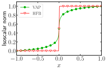
Figure 1: Evolution of the isoscalar norm as a function of the mixing parameter $x$ in Eq. (1), obtained in Ref. [4] using the HFB (open symbols) and VAP methods (full symbols).

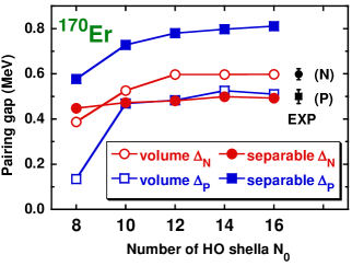
Figure 2: Convergence of the neutron and proton pairing gaps in ¹⁷⁰Er with increasing number of the HO shells $N_{0}$, determined for the zero-range volume and separable pairing interaction.

3 Separable pairing interaction

In this Section, we present a detailed derivation of the matrix elements of the separable interaction in a Cartesian basis. The separable interaction has the general form

$$\begin{split}\hat{V}(\mathbf{r_{1}},\mathbf{r_{2}};\mathbf{r_{1}}^{\prime},\mathbf{r_{2}}^{\prime})&=-\delta(X-X^{\prime})\delta(Y-Y^{\prime})\delta(Z-Z^{\prime})P(x)P(y)P(z)P(x^{\prime})P(y^{\prime})P(z^{\prime})\\ &\times[\tilde{W}\hat{\mathbb{1}}+\tilde{B}\hat{P}^{\sigma}-\tilde{H}\hat{P}^{\tau}-\tilde{M}\hat{P}^{\sigma}\hat{P}^{\tau}]\;,\end{split}$$ (2)

where $\mathbf{r_{i}}=(x_{i},y_{i},z_{i})$, $x=x_{1}-x_{2}$ and $X=\frac{1}{2}(x_{1}+x_{2})$ are the relative and center-of-mass coordinates (equivalent symbols hold for the other Cartesian directions). For the form factor, we chose a simple Gaussian as

$$P(x)=\frac{1}{\sqrt{\pi}a}e^{-x^{2}/a^{2}}\;,$$ (3)

where $a=1.232$ fm is the range [12]. Symbols $\tilde{W}$, $\tilde{B}$, $\tilde{H}$, and $\tilde{M}$ denote adjustable parameters (Wigner, Bartlett, Heisenberg, and Majorana coupling constants), $\hat{\mathbb{1}}$ is the identity operator, and $\hat{P}^{\sigma}$ and $\hat{P}^{\tau}$ are spin and isospin exchange operators, respectively. Because form factor (3) is symmetric in space coordinates, only parameters $\tilde{W}$ and $\tilde{B}$ are independent.

To calculate the matrix elements of interaction (2), we define the basis of two particles coupled to total spin $S=0$ as

$$|n_{1}n_{2},S=0\rangle=\phi_{n_{1}}(x_{1},b)\phi_{n_{2}}(x_{2},b)|S=0\rangle\;,$$ (4)

where $\phi_{n}(x,b)$ is the harmonic oscillator (HO) wavefunction with quantum number $n$ and oscillator constant $b$,

$$\phi_{n}(x,b)=b^{1/2}H_{n}^{(0)}(bx)e^{-b^{2}x^{2}/2}\;.$$ (5)

In Eq. (5), we used a normalized version $H_{n}^{(0)}(x)$ of the Hermite polynomials $H_{n}(x)$, defined as

$$H_{n}^{(0)}(x)=(\sqrt{\pi}2^{n}n!)^{-1/2}H_{n}(x)\;.$$ (6)

We now evaluate the matrix elements in the new basis as

$$\langle n_{1}^{\prime}n_{2}^{\prime},S=0|\hat{V}|n_{1}n_{2},S=0\rangle=-I_{x}I_{y}I_{z}(\tilde{W}-\tilde{B})\;,$$ (7)

where $I_{x}$ is defined as

$$I_{x}(n_{1}n_{2};n^{\prime}_{1}n^{\prime}_{2})=\int dx_{1}dx_{2}dx^{\prime}_{1}dx^{\prime}_{2}\delta(X-X^{\prime})P(x)P(x^{\prime})\phi_{n_{1}}(x_{1},b)\phi_{n_{2}}(x_{2},b)\phi_{n^{\prime}_{1}}(x^{\prime}_{1},b)\phi_{n^{\prime}_{2}}(x^{\prime}_{2},b)\;,$$ (8)

and similarly for $I_{y}$ and $I_{z}$. To calculate $I_{x}$, it is convenient to express the two-particle basis in the center of mass coordinates,

$$\phi_{n_{1}}(x_{1},b)\phi_{n_{2}}(x_{2},b)=\sum_{nN}M_{n_{1}n_{2}}^{nN}\phi_{n}(\tilde{x},b)\phi_{N}(\tilde{X},b)\;,$$ (9)

where $\tilde{x}=\frac{x}{\sqrt{2}}$, $\tilde{X}=\sqrt{2}X$, and symbol $M_{n_{1}n_{2}}^{nN}=\langle n_{1}n_{2}|nN\rangle$ denotes the Moshinsky coefficients, which are given by the expression [13]

$$M_{n_{1}n_{2}}^{nN}=\frac{\sqrt{n_{1}!n_{2}!n!N!}}{2^{\frac{n+N}{2}}}\delta_{n_{1}+n_{2},n+N}\sum_{k=\max(0,n_{1}-n)}^{\min(N,n_{1})}\frac{(-1)^{n-n_{1}+k}}{k!(N-k)!(n_{1}-k)!(n-n_{1}+k)!}\;.$$ (10)

We now obtain a new expression for $I_{x}$,

$$\begin{split}I_{x}(n_{1}n_{2};n^{\prime}_{1}n^{\prime}_{2})=&\sum_{n,n^{\prime},N,N^{\prime}}M_{n_{1}n_{2}}^{nN}M_{n^{\prime}_{1}n^{\prime}_{2}}^{n^{\prime}N^{\prime}}\\ &\times\int dxdx^{\prime}dXdX^{\prime}\delta(X-X^{\prime})P(x)P(x^{\prime})\phi_{n}(\tilde{x},b)\phi_{n^{\prime}}(\tilde{x}^{\prime},b)\phi_{N}(\tilde{X},b)\phi_{N^{\prime}}(\tilde{X^{\prime}},b)\;,\end{split}$$ (11)

The integral over the coordinates $X,X^{\prime}$ can be performed analytically, and gives

$$\begin{split}&\int dXdX^{\prime}\delta(X-X^{\prime})\phi_{N}(\tilde{X},b)\phi_{N^{\prime}}(\tilde{X^{\prime}},b)=\frac{1}{\sqrt{2}}\delta_{NN^{\prime}}\;,\end{split}$$ (12)

where we used the normalization condition of the Hermite polynomials $H_{n}^{(0)}(x)$ [14]. Inserting this result into Eq. (11), we get

$$I_{x}(n_{1}n_{2};n^{\prime}_{1}n^{\prime}_{2})=\frac{1}{\sqrt{2}}\sum_{n,n^{\prime},N}M_{n_{1}n_{2}}^{nN}M_{n^{\prime}_{1}n^{\prime}_{2}}^{n^{\prime}N}\int dxdx^{\prime}P(x)P(x^{\prime})\phi_{n}(\tilde{x},b)\phi_{n^{\prime}}(\tilde{x}^{\prime},b)\;,$$ (13)

which can be written as

$$I_{x}(n_{1}n_{2};n^{\prime}_{1}n^{\prime}_{2})=\frac{1}{\sqrt{2}}\sum_{n,n^{\prime},N}M_{n_{1}n_{2}}^{nN}M_{n^{\prime}_{1}n^{\prime}_{2}}^{n^{\prime}N}W(n)W(n^{\prime})\;,$$ (14)

where $W(n)=\int dxP(x)\phi_{n}(\tilde{x},b)$. Using the properties of the HO wavefunction, this integral can be expressed as

$$W(n)=\frac{\sqrt{2}}{\sqrt{\pi ba^{2}}}\int dte^{-2t^{2}/(ba)^{2}}H_{n}^{(0)}(t)e^{-\frac{t^{2}}{2}}\;,$$ (15)

where we changed the integration variable to $t=bx/\sqrt{2}$. Then using the following identity

$$\int_{-\infty}^{+\infty}duH_{2m}^{(0)}(\alpha u)e^{-u^{2}}=\pi^{1/4}\frac{\sqrt{(2m)!}}{m!}\left(\frac{\alpha^{2}-1}{2}\right)^{m}\;,$$ (16)

we obtain the final result

$$W(n)=\frac{2\pi^{-1/4}\sqrt{b}}{\sqrt{a^{2}b^{2}+4}}\frac{\sqrt{n!}}{(n/2)!}\bigg{(}\frac{a^{2}b^{2}-4}{2a^{2}b^{2}+8}\bigg{)}^{n/2}\;.$$ (17)

We observe that the sum over $n,n^{\prime}$ in Eq. (13) can be further reduced by using the fact that the Moshinsky coefficients will be zero unless $n=n_{1}+n_{2}-N$ and $n^{\prime}=n^{\prime}_{1}+n^{\prime}_{2}-N$. It is convenient to rewrite the final expression of the matrix elements as

$$I_{x}(n_{1}n_{2};n^{\prime}_{1}n^{\prime}_{2})=\frac{1}{\sqrt{2}}\sum_{N=0}^{n_{1}+n_{2}}G(N,n_{1},n_{2})G(N,n^{\prime}_{1},n^{\prime}_{2})\;,$$ (18)

where

$$G(N,n_{1},n_{2})=M_{n_{1}n_{2}}^{n_{1}+n_{2}-N,N}W(n_{1}+n_{2}-N)\;.$$ (19)

It is worth noting that a similar derivation of matrix elements in Cartesian space has already been given in Ref. [15], however, in their derivation we have found several errors and missing factors in the final expressions. In addition, an alternative derivation of the analogous matrix elements of more general separable interactions was given in Ref. [16].

4 Pairing gaps

We tested our derivations and implementation in the code hfodd (v2.91a) [17, 18] by comparing our results with the ones obtained by the code hosphe [19] – an HFB solver in spherical symmetry, which also contains an implementation of the same separable interaction in the pairing channel. For a fixed number of shells, we reproduced the results of Fig. 1 of Ref. [12] up to an eV accuracy, thus obtaining a very strong test on the correctness of our results.

In this work, we present an example of calculations performed for the chain of deformed Erbium isotopes. First, using the SLy4 functional [20] in the particle-hole channel, we roughly adjusted parameter $\tilde{W}=-\tilde{B}=-300$ MeV fm³, Eq. (7), to reproduce the values of experimental neutron, $\Delta_{N}$, and proton, $\Delta_{P}$, pairing gaps in ¹⁷⁰Er. In Fig. 2, we plotted the calculated ¹⁷⁰Er neutron and proton pairing gaps as functions of the number of the HO shells $N_{0}$. We observe that the results converge nicely as a function of $N_{0}$, and we can consider that at $N_{0}=14$ the pairing gaps are sufficiently converged [21]. We note that the charge-symmetric separable pairing interaction used here is not capable of reproducing the experimental values of the ¹⁷⁰Er neutron and proton pairing gaps simultaneously.

In the same figure, we also report the analogous convergence obtained for a simple charge-symmetric volume contact pairing interaction adjusted to the same experimental data, which for the equivalent-spectrum cut-off of 60 MeV gave the strength of $V_{0}=-195$ MeV fm³. Contrary to typical applications of the volume pairing, where different strengths are used for neutrons and protons, cf. Ref. [22], here the experimental values of the ¹⁷⁰Er neutron and proton pairing gaps are perfectly reproduced by the charge-symmetric parametrization.

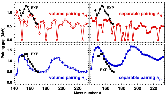
Figure 3: Calculated neutron (upper panels) and proton (lower panels) pairing gaps in Erbium isotopes determined for the zero-range volume (left panels) and separable (right panels) pairing interaction for $N_{0}=14$ HO shells. Neutron and proton experimental values are calculated as averages of the three-point mass staggering centered on two adjacent odd isotopes and isotones, respectively.

Having adjusted the strengths of the two pairing interactions, in Fig. 3 we compare the isotopic behaviour of the calculated pairing gaps in Erbium isotopes. We observe that the separable pairing tends to give a weaker pairing for neutrons and a stronger for protons than the volume pairing. It is interesting to note that in some nuclei the separable interaction leads to a vanishing neutron gap, whereas the volume interaction may still give there a non-zero value of $\Delta_{N}\approx 0.5$ MeV. Since Erbium nuclei are deformed (apart from the semi-magic isotopes), we checked that the values of the quadrupole moment, obtained for both interactions, are practically the same.

5 Conclusions

In this contribution, we briefly discussed the question of how to observe and describe, within a simple SO(8) model, the coexistence of isoscalar and isovector pairs by employing mean-field wave functions with all relevant broken symmetries restored. In the perspective of applying such a procedure to the realistic cases of finite nuclei, we presented a detailed derivation of matrix elements of a separable finite-range interaction in Cartesian basis, where we corrected errors found in the literature derivations. To illustrate a practical implementation in the 3D code hfodd, we also presented a series of systematic HFB calculations in Erbium isotopes, and we compared the results with those obtained using a simpler zero-range volume interaction.

This work was partially supported by the STFC Grants No. ST/M006433/1 and No. ST/P003885/1, and by the Polish National Science Centre under Contract No. 2018/31/B/ST2/02220. We acknowledge the CSC-IT Center for Science Ltd., Finland, for the allocation of computational resources.

References

References

- [1] Broglia R A and Zelevinsky V 2013 Fifty years of nuclear BCS: pairing in finite systems (World Scientific)
- [2] Bardeen J, Cooper L N and Schrieffer J R 1957 Physical Review 108 1175
- [3] Frauendorf S and Macchiavelli A 2014 Prog. Part. Nucl. Phys. 78 24–90
- [4] Romero A, Dobaczewski J and Pastore A 2019 Physics Letters B 795 177 – 182
- [5] Bender M, Heenen P H and Reinhard P G 2003 Reviews of Modern Physics 75 121
- [6] Pang S C 1969 Nuclear Physics A 128 497–526
- [7] Kota V and Alcarás J C 2006 Nucl. Phys. A 764 181–204
- [8] Duguet T 2004 Physical Review C 69 054317
- [9] Tian Y, Ma Z and Ring P 2009 Physics Letters B 676 44–50
- [10] Bulgac A and Yu Y 2002 Physical Review Letters 88 042504
- [11] Bertsch G and Esbensen H 1991 Annals of Physics 209 327–363
- [12] Veselỳ P, Dobaczewski J, Michel N and Toivanen J 2011 Journal of Physics: Conference Series vol 267 (IOP Publishing) p 012027
- [13] Dobaczewski J, Satuła W, Carlsson B, Engel J, Olbratowski P, Powałowski P, Sadziak M, Sarich J, Schunck N, Staszczak A et al. 2009 Computer Physics Communications 180 2361–2391
- [14] Abramowitz M and Stegun I A 1965 Handbook of mathematical functions with formulas, graphs, and mathematical table US Department of Commerce (National Bureau of Standards Applied Mathematics series 55)
- [15] Nikšić T, Ring P, Vretenar D, Tian Y and Ma Z y 2010 Physical Review C 81 054318
- [16] Robledo L M 2010 Physical Review C 81 044312
- [17] Schunck N, Dobaczewski J, Satuła W, Ba̧czyk P, Dudek J, Gao Y, Konieczka M, Sato K, Shi Y, Wang X and Werner T 2017 Comp. Phys. Commun. 216 145 – 174
- [18] Dobaczewski J 2019 et al., to be published
- [19] Carlsson B, Dobaczewski J, Toivanen J and Veselỳ P 2010 Computer Physics Communications 181 1641–1657
- [20] Chabanat E, Bonche P, Haensel P, Meyer J and Schaeffer R 1997 Nuclear Physics A 627 710–746
- [21] Bender M, Rutz K, Reinhard P G and Maruhn J A 2000 The European Physical Journal A 8 59–75
- [22] Kortelainen M, Lesinski T, Moré J, Nazarewicz W, Sarich J, Schunck N, Stoitsov M V and Wild S 2010 Phys. Rev. C 82 024313