Derive the Born’s rule from environment-induced stochastic dynamics of wave-functions in an open system

Abstract

The lack of superposition of different position states or the emergence of classicality in macroscopic systems have been a puzzle for decades. Classicality exists in every measuring apparatus, and is the key for understanding what can be measured in quantum theory. Different theories have been proposed, including decoherence, einselection and the spontaneous wave-function collapse, with no consensus reached up to now. In this paper, we propose a stochastic dynamics for the wave-function in an open system (e.g. the measuring apparatus) that interacts with its environment. The trajectory of wave-function is random with a well-defined probability distribution. We show that the stochastic evolution results in the wave-function collapse and the Born’s rule for specific system-environment interactions. While it reproduces the unitary evolution governed by the Schrödinger equation when the interaction vanishes. Our results suggest that it is the way of system interacting with environment that determines whether quantum superposition dominates or classicality emerges.

1 Introduction

Quantum mechanics is exceedingly successful in explaining the experiments, with no conflict being found up to now. But ever since its born, the theory is debated for its inability to explain the familiar classical world where the measuring apparatus and observers live in. Einstein criticized that the theory does not ”decide what can be observed”. Various theories have been proposed to fix this problem, including Bohmian mechanics Bohm , many-worlds interpretation Everett , decoherence and einslection Zurek03 , and spontaneous wave-function collapse models Bassi13 .

The debate stems from an axiom of quantum mechanics - the Born’s rule. It states Nielsen that a measurement (a projection-valued measurement) in mathematics defines an orthogonal basis of the Hilbert space, into which the wave-function is decomposed:

$$\ket{\phi}=\sum_{s}\alpha_{s}\ket{\phi_{s}}.$$ (1)

The probability of the wave-function collapsing into $\ket{\phi_{s}}$ is $P_{s}=\left|\alpha_{s}\right|^{2}$. $\{\ket{\phi_{s}}\}$ is the eigenbasis of the observable operator. But quantum mechanics does not clarify how $\{\ket{\phi_{s}}\}$ is connected to the measuring apparatus. Imagine an experiment in which we need to measure the position of an electron. Why do we know that we are measuring the position, but not something else like the momentum? Whether we are measuring the position or momentum is determined by the measuring apparatus. Therefore, quantum mechanics cannot be self-consistent without giving explicitly how to determine $\{\ket{\phi_{s}}\}$ from the description of measuring apparatus.

This problem was noticed in the early days of quantum mechanics. In the Copenhagen interpretation Bohr28 , there is a border between quantum and classical worlds. The microscopic world obeys quantum laws. But the macroscopic world including the measuring apparatus and observers has to be described classically. A classical world is necessary for determining whether the position or momentum is measured. This is of course unsatisfying, because the border is defined ambiguously. Many different approaches have been proposed to replace the Copenhagen interpretation. For each approach, how to derive the Born’s rule is a crucial question to answer.

A proof of the Born’s rule was given by Gleason in 1957 Gleason . But it is purely mathematical without addressing the foundation of quantum mechanics. Everett Everett proposed the many-worlds interpretation, in which both the microscopic system and macroscopic measuring apparatus are parts of the universe with the latter being described by a pure wave function. This wave function evolves according to the Schrödinger equation, being totally deterministic. To answer why the specific set of vectors $\{\ket{\phi_{s}}\}$ are chosen during the measuring process, decoherence Zeh70 and einselection Zurek81 ; Zurek82 were introduced. Within a measurement, the microscopic system is entangled with the measuring apparatus. At the same time, the interaction with environment singles out a preferred basis in the Hilbert space of the measuring apparatus, dubbed the pointer states. The pointer states remains untouched in the interaction with environment, while their superpositions decohere. And the environment acquires and transmits redundant information about the pointer states Zurek03 . The pointer states correspond to the classical states in our familiar world, forming the preferred basis in the Born’s rule. To answer why the probability is $\left|\alpha_{s}\right|^{2}$, Deutsch Deutsch suggested an argument based on the decision theory. His argument was debated by Barnum Barnum but then developed by Saunders Saunders and Wallace Wallace03 ; Wallace07 . Later on, Zurek Zurek03PRL ; Zurek05 ; Schlosshauer proposed a different derivation of the Born’s rule based on the environment-assisted invariance. Either Deutsch’s or Zurek’s arguments remain controversial up to today Rae ; Herbut ; Mandolesi18 ; Mandolesi19 ; Mandolesi20 . The many-worlds interpretation and the derivation of the Born’s rule based on it need no modification to quantum mechanics, and are then welcome because quantum theory has been verified by many experiments. However, it does not really explain how the superposition between measuring apparatus and environment is destroyed in a single measurement Bassi13 . And one has to solve the Schrödinger equation and know the universe wave-function in the distant future before defining the pointer states at present. It is not clear whether such-defined pointer states exist when the interaction between measuring apparatus and environment is as complicated as in real world, or how to define the pointer states when the interaction is changing with time.

The hidden-variable theories circumvent the quantum measurement problem by assuming the existence of pre-quantum (sub-microscopic) degrees of freedom which are deterministic Hooft ; Genovese . The pre-quantum state evolves classically with the quantum mechanics being its statistical description. The Bohmian mechanics Bohm52a ; Bohm52b is a hidden-variable theory. According to it, the distribution of the pre-quantum states will always obey the Born’s rule once if the initial positions of the particles have a Born-rule distribution. Recently, the timescale for dynamical relaxation to the Born’s rule was analyzed as the initial distribution deviates from it Towler . And new hidden-variable theories were suggested (see Ref. Khrennikov14 for an example). But how to observe the pre-quantum degrees of freedom remains a problem in these theories.

For explaining the emergence of measuring apparatus’ classicality, the spontaneous collapse models modify the quantum mechanics in a way so that the wave-function collapse is spontaneous and objective. The Ghirardi-Rimini-Weber (GRW) model Ghirardi86 , quantum mechanics with universal position localization Bassi05 , and continuous spontaneous localization Pearle89 ; Ghirardi90 (CSL) model are in this family. In these models, the wave-function evolution does not follow the deterministic Schrödinger equation any more, but is stochastic. For a particle of macroscopic mass, the stochastic equation results in spontaneous localization in real space. The solution is a Gaussian wave package Bassi05 with its center having a random trajectory. If the initial state is a superposition of wave packages at different positions, to which position the wave-function collapses into is probabilistic. And the distribution was shown to obey the Born’s rule. The spontaneous collapse models are self-consistent and falsifiable. Due to the development of optomechanics and matter-wave interferometry, experiments have been carried out to put bounds on the parameters of spontaneous collapse models Bassi13 ; Arndt14 ; Pontin19 . And researchers keep on raising new proposals for testing them Yin13 ; Bahrami14 ; Nimmrichter14 ; Diosi14 ; Goldwater15 . But there exist difficulties in generalizing these models to a relativistic theory, which limit their application Jones19 .

There were attempts to explain the classicality of the measuring apparatus in the context of orthodox quantum mechanics. Kraus Kraus81 ; Kraus85 proposed a quantum-mechanical model of a macroscopic counter that monitors the decay of an unstable particle. His model was improved by Braun Braun92 and Urbanowski Urbanowski93 . In the quantum optics community, the quantum trajectory theory Brun02 ; Jacobs06 was developed to describe open quantum systems subjected to continuous measurement. The quantum trajectory formalism, which is based on a continuous stochastic process, was shown to be consistent with the Born’s rule Patel17 . But the theory does not really solve the fundamental measurement problem. Instead, it shifts the quantum-classical border to the dynamics of the amplifier.

In addition to above approaches, some authors derived the Born’s rule from the time reversal symmetry Ilyin15 , or proved that the alternatives to Born’s rule violate the compositional principle of purification and local tomography Galley16 ; Galley18 . The experimental test of the Born’s rule with three-path interference was also proposed and carried out Sorkin94 ; Sinha10 ; Quach17 ; Pleinert20 .

Up to now, the quantum measurement problem and the origination of the Born’s rule are not solved yet. New approach is still worth trying. In this paper, we propose an environment-induced stochastic dynamics of wave-functions. In our assumptions, the wave-function collapse is objective. The evolution of wave-function in an open system is a stochastic process but not deterministic. The Born’s rule is not an axiom, instead, it must be derived as a result of the stochastic dynamics. At this point, we agree with the spontaneous collapse models. On the other hand, the wave-function collapse is due to the interaction with environment (environment-induced), thereafter, an isolated system experiences no wave-function collapse and follows the same unitary evolution governed by the Schrödinger equation. We do not need to worry about a conflict to experiments that have been well explained by orthodox quantum mechanics for isolated systems. At this point, we inherit the spirit of einselection.

The paper is arranged as follows. We propose the stochastic dynamics and discuss its properties in Sec. 2. In Sec. 3, we introduce the central spin model. Sec. 4 explains how the Born’s rule arises from the stochastic dynamics. Sec. 5 presents the numerical results and discusses the conditions of the Born’s rule. Sec. 6 summarizes our model and results.

2 Environment-induced stochastic dynamics of wave-functions

In this section, we propose the stochastic dynamics of wave-functions in an open system. When we say system in this paper, we mean a measuring apparatus in which one can observe the collapse of wave-functions and the emergence of classicality.

The system and its environment combine into an isolated universe, whose evolution is governed by the Schrödinger equation. The total Hamiltonian is

$$\hat{H}=\hat{H}_{E}+\hat{H}_{S}+\hat{V}_{SE},$$ (2)

where $\hat{H}_{E}$ and $\hat{H}_{S}$ are the Hamiltonians for environmental and system’s degrees of freedom, respectively, and $\hat{V}_{SE}$ is the interaction between them. We use $\mathcal{H}_{E}$ and $\mathcal{H}_{S}$ to denote the Hilbert space for the environment and system, respectively, and $\ket{n}$ to denote the eigenstate of $\hat{H}_{E}$ with the energy $E_{n}$. Here we assume no degeneracy and the set $\left\{\left(\ket{n},E_{n}\right)\right\}$ is uniquely defined, which is a common simplifying assumption for the environment that avoids the complications associated to continuous spectra and degeneracy.

Now suppose that at some given time $t_{0}$, the wave-function of system is $\ket{\phi}$. We hope to predict the distribution of wave-functions at arbitrarily later time $t$. For this purpose, we need also know the wave-function of the environment at $t_{0}$. The environment is not necessarily in a pure state, but can also be in a mixed state. Without loss of generality, we suppose that the environment is in the state $\ket{\gamma}$ with the probability $f_{\gamma}$. The distribution $f_{\gamma}$ reflects the uncertainty in our knowledge of the environment. The environment is in a pure state if $f_{\gamma}$ is a $\delta$-function.

The main assumption in this paper is that, at the time $t\geq t_{0}$, the wave-function of the system is

$$\ket{\phi_{n,\gamma}(t)}=\frac{1}{\sqrt{g_{n,\gamma}}}\bra{n}e^{-i\left(t-t_{0}\right)\hat{H}}\ket{\gamma}\otimes\ket{\phi}$$ (3)

with the probability $P_{n,\gamma}$. Here $n$ and $\gamma$ denote the final and initial environmental states, respectively. Notice that $\ket{\gamma}\otimes\ket{\phi}$ is indeed the wave-function of the whole universe at $t_{0}$, and $e^{-i\left(t-t_{0}\right)\hat{H}}\ket{\gamma}\otimes\ket{\phi}$ gives the trajectory of the universe wave-function in the Hilbert space $\mathcal{H}_{E}\otimes\mathcal{H}_{S}$. The nomalization factor reads $g_{n,\gamma}(t)=\left\|\bra{n}e^{-i\left(t-t_{0}\right)\hat{H}}\ket{\gamma}\otimes\ket{\phi}\right\|^{2}$, where $\left\|\cdot\right\|$ denotes the inner product of a vector with itself. The probability distribution is expressed as

$$P_{n,\gamma}(t)=f_{\gamma}\ g_{n,\gamma}(t).$$ (4)

The set of pairs $\left\{\left(\ket{\phi_{n,\gamma}(t)},P_{n,\gamma}(t)\right)\right\}$ defines a stochastic process in the Hilbert space $\mathcal{H}_{S}$. The system’s wave-function has a random trajectory. It can take different possible values $\ket{\phi_{n,\gamma}(t)}$ at a certain time, where $n$ and $\gamma$ are variables. The probability $P_{n,\gamma}(t)$ must be normalized at arbitrary $t\geq t_{0}$. It is easy to verify $\sum_{n,\gamma}P_{n,\gamma}=1$.

A physically well-defined evolution should be continuous with time. The above stochastic process is indeed continuous. Especially, at $t=t_{0}$, Eqs. (3-4) tell us $\ket{\phi_{n,\gamma}(t)}\equiv\ket{\phi}$ (expect for an unphysical global phase) for arbitrary $n$ and $\gamma$, thereafter, the system is in the state $\ket{\phi}$ with $100\%$ probability. This is consistent with our initial condition.

For an isolated system ($\hat{V}_{SE}=0$), Eqs. (3-4) tell us that the wave-function is $e^{-i(t-t_{0})\hat{H}_{S}}\ket{\phi}$ with $100\%$ probability except for an unphysical global phase. This is exactly the solution of the Schrödinger equation. For an open system ($\hat{V}_{SE}\neq 0$), we also find a correspondence between quantum mechanics and our model. Eqs. (3-4) give the distribution of the wave-functions. On the other hand, quantum mechanics predicts the reduced density matrix at a given time by tracing out the environmental degrees of freedom, which is $\hat{\rho}_{S}(t)=\text{Tr}_{E}\hat{\rho}(t)$ with the universe density matrix expressed as $\hat{\rho}(t)=\sum_{\gamma}f_{\gamma}\ket{\Psi_{\gamma}(t)}\bra{\Psi_{\gamma}(t)}$ and the universe wave function as $\ket{\Psi_{\gamma}(t)}=e^{-i\left(t-t_{0}\right)\hat{H}}\ket{\gamma}\otimes\ket{\phi}$. From Eqs. (3) and (4), it is easy to prove

$$\hat{\rho}_{S}(t)=\sum_{n,\gamma}P_{n,\gamma}(t)\ket{\phi_{n,\gamma}(t)}\bra{\phi_{n,\gamma}(t)}.$$ (5)

Eq. (5) is just the von Neumann’s definition of density matrix. Therefore, our equations predict the same reduced density matrix as quantum mechanics, but contain more information, because the decomposition of $\hat{\rho}_{S}(t)$ into an ensemble of wave functions is not unique (the basis can be chosen arbitrarily). This non-uniqueness reflects the disability of quantum mechanics in explaining the emergence of classical states.

We like to mention that $\ket{\phi_{n,\gamma}(t)}$ at different $\left(n,\gamma\right)$ are not orthogonal to each other. Therefore, they do not form a basis of $\mathcal{H}_{S}$, and must be distinguished from the pointer states in einselection.

It is worth emphasizing that our assumption relies on a non-symmetric prescription for the evolution of environment and system. The dynamical law (3) has to distinguish between the environment on one hand and the system on the other. According to our assumption, the environment contains the observer. For a specific observer, he can always tell which party is the system and which is the environment. The trajectory of the system’s state is interesting to the observer, but that of the environment is not.

3 Central spin model

For a generic Hamiltonian, the wave function and probability defined by Eqs. (3) and (4) are difficult to calculate. To obtain a paradigm of the stochastic process defined above, we consider the system to be as simple as a spin-$1/2$ particle. And we can neglect the system’s Hamiltonian, if we only study the collapse of its wave function. The environment has much more degrees of freedom than the system. To keep the model solvable, we treat the environment as a collection of $N$ spins without interaction between each other. The environmental spins and the system spin have an interaction, which serves as the reason for the wave-function collapse.

Such a model is often called the central spin model. The model studied next is similar to that studied in Ref. Zwolak16 . The environmental Hamiltonian is

$$\hat{H}_{E}=\mu\sum_{j=1}^{N}\hat{\sigma}_{j}^{z},$$ (6)

where $\hat{\sigma}_{j}^{z}$ is the Pauli matrix of the $j$-th spin. It is equivalent to say that all the environmental spins are in $z$-direction for an eigenstate. No generality is lost, because we can always define the direction of each environmental spin in its own inner space as the ”$z$-direction”. The eigenstate of $\hat{H}_{E}$ is written as $\ket{n}=\ket{s_{1},\cdots s_{N}}$ with $s_{j}=\pm 1$ denoting the spin-up and spin-down states, respectively. The interaction between system and environment is

$$\hat{V}_{SE}=\sum_{j=1}^{N}\hat{\sigma}_{S}^{z}\left(h_{j}\hat{\sigma}_{j}^{x}+\nu\hat{\sigma}_{j}^{z}\right),$$ (7)

where $\hat{\sigma}_{S}^{z}$ is the Pauli matrix of the central spin. The coupling is in the longitudinal direction together with a component $h_{j}$ in the transversal direction.

We set $t_{0}=0$ as the initial time. And the environment is in thermal equilibrium, i.e., the environment is in the state $\ket{n}$ with probability $f_{n}=e^{-\beta E_{n}}/Z$ with $Z=\sum_{n}e^{-\beta E_{n}}$ the partition function and $\beta$ the inverse of temperature. The dynamics that we are interested in is indeed independent of $f_{n}$ and $\beta$. The initial wave-function of the system is generally expressed as

$$\ket{\phi}=\alpha_{\uparrow}\ket{\uparrow}+\alpha_{\downarrow}\ket{\downarrow},$$ (8)

where $\ket{\uparrow}$ and $\ket{\downarrow}$ are the eigenstates of $\hat{\sigma}_{S}^{z}$ and $\left|\alpha_{\uparrow}\right|^{2}+\left|\alpha_{\downarrow}\right|^{2}=1$ is the normalization condition. Here $\ket{\uparrow}$ and $\ket{\downarrow}$ are the two classical states. According to the Born’s rule, the wave-function of the system should collapse into them with the probabilities $\left|\alpha_{\uparrow}\right|^{2}$ and $\left|\alpha_{\downarrow}\right|^{2}$, respectively.

Following Eqs. (3-4), we obtain the distribution of wave-functions at arbitrary $t>t_{0}$. Using $\left(n^{\prime},n\right)=\left(\left(s^{\prime}_{1},s_{1}\right),\cdots,\left(s^{\prime}_{N},s_{N}\right)\right)$ to denote a pair of initial and final environmental states, we find the system’s wave function to be

$$\ket{\phi_{n^{\prime},n}(t)}=\frac{\displaystyle\alpha_{\uparrow}G^{\uparrow}_{n^{\prime},n}}{\sqrt{g_{n^{\prime},n}(t)}}\ket{\uparrow}+\frac{\displaystyle\alpha_{\downarrow}G^{\downarrow}_{n^{\prime},n}}{\sqrt{g_{n^{\prime},n}(t)}}\ket{\downarrow}$$ (9)

with the probability $P_{n^{\prime},n}(t)=f_{n}g_{n^{\prime},n}(t)$. The normalization factor is

$$g_{n^{\prime},n}=\left|\alpha_{\uparrow}\right|^{2}\left|G^{\uparrow}_{n^{\prime},n}\right|^{2}+\left|\alpha_{\downarrow}\right|^{2}\left|G^{\downarrow}_{n^{\prime},n}\right|^{2},$$ (10)

where $G^{\uparrow/\downarrow}_{n^{\prime},n}=\displaystyle\prod_{j=1}^{N}G^{\uparrow/\downarrow}_{j}$ are the spin-up and spin-down significances, respectively. And $G^{\uparrow/\downarrow}_{j}=\bra{s^{\prime}_{j}}e^{-it\left(\left(\mu\pm\nu\right)\hat{\sigma}^{z}_{j}\pm h_{j}\hat{\sigma}^{x}_{j}\right)}\ket{s_{j}}$ is the significance contributed by the $j$-th environmental degree of freedom. Note that $\left|G^{\uparrow/\downarrow}_{j}\right|^{2}$ depends only upon $s_{j}s^{\prime}_{j}$, but is independent of the initial environmental state.

3.1 Solutions without wave-function collapse

Let us first consider special choices of parameters to obtain an analytical solution. If $h_{j}\equiv 0$ and the environment is at zero temperature, the wave-function is $\ket{\phi(t)}=\alpha_{\uparrow}e^{-itE_{gs}}\ket{\uparrow}+\alpha_{\downarrow}e^{itE_{gs}}\ket{\downarrow}$ with $100\%$ probability, where $E_{gs}$ is the ground-state energy of the environment.

Another choice is $\nu=0$ and $h_{j}\equiv h$ being a constant. Because the environmental degrees of freedom (the universe) are much more than the system’s, it is reasonable to take the large-environment limit ($N\to\infty$). In this limit and for almost all the time, the system’s wave-function is $\alpha_{\uparrow}\ket{\uparrow}+\alpha_{\downarrow}\ket{\downarrow}$ or $\alpha_{\uparrow}\ket{\uparrow}-\alpha_{\downarrow}\ket{\downarrow}$ with equal probabilities. Only at the specific times $t=m\pi/\sqrt{\mu^{2}+h^{2}}$ with $m$ an arbitrary integer, the wave-function recovers to its initial value with $100\%$ probability. In both choices, there is no wave-function collapse, and the superposition principle of quantum mechanics is preserved.

4 The Born’s rule

In this section, we show how the classicality and the Born’s rule emerges from Eqs. (3) and (4) in the central spin model. Recall that the spin-up significance is $\left|G^{\uparrow}_{n^{\prime},n}\right|^{2}=\prod_{j=1}^{N}\left|G^{\uparrow}_{j}\right|^{2}$ and the spin-down significance is $\left|G^{\downarrow}_{n^{\prime},n}\right|^{2}=\prod_{j=1}^{N}\left|G^{\downarrow}_{j}\right|^{2}$. We choose $\mu+\nu=1$ as the unit of energy and its inverse the unit of time. The significance on the $j$-th environmental degree of freedom is

$$\left|G^{S}_{j}\right|^{2}=\bigg{\{}\begin{array}[]{cc}\cos^{2}\left(\omega^{S}_{j}t\right)+\sin^{2}\left(\omega^{S}_{j}t\right)r^{S}_{j},&d_{j}=1\\[14.22636pt] \sin^{2}\left(\omega^{S}_{j}t\right)\left(1-r^{S}_{j}\right),&d_{j}=-1.\end{array}$$ (11)

Here $S=\uparrow,\downarrow$ denotes the spin-up and spin-down states of the system, respectively. $d_{j}=s_{j}s^{\prime}_{j}=\pm 1$ represents flip or no-flip of the $j$-th environmental spin, respectively. $\omega^{\uparrow}_{j}=\sqrt{1+h^{2}_{j}}$ is the frequency and $r^{\uparrow}_{j}=1/\left(1+h_{j}^{2}\right)$ is the ratio for spin-up state, while $\omega^{\downarrow}_{j}=\sqrt{\left(\mu-\nu\right)^{2}+h^{2}_{j}}$ and $r^{\downarrow}_{j}=\left(\mu-\nu\right)^{2}/\left(\left(\mu-\nu\right)^{2}+h_{j}^{2}\right)$ are for spin-down state.

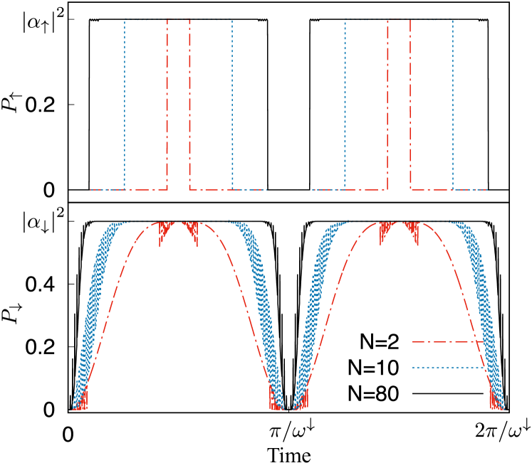
Figure 1: (Color online) The evolution of $P_{\uparrow}$ and $P_{\downarrow}$ for different $N$. We choose $\mu-\nu=0$, $h_{j}=0.01$ being a constant, and $\left|\alpha_{\uparrow}\right|^{2}=0.4$. The error is $\epsilon=10^{-3}$.

We notice $\left|G_{j}^{\uparrow}\right|^{2}_{d_{j}=1}+\left|G_{j}^{\uparrow}\right|^{2}_{d_{j}=-1}\equiv 1$. With $j$ varying from $1$ to $N$, there are $N$ pairs of positive numbers with each pair summing up to unity. The spin-up significance is obtained by choosing one number from each pair according to whether the involved degree of freedom is flipped or not, and then multiplying all the $N$ numbers. The spin-down significance is obtained in the same way. If $N$ is large, depending on how unity is decomposed into two positive numbers for each $j$, the ratio of spin-up to spin-down significance can be close to zero or very large (think about the fact $\left(0.9\times 0.1\right)^{N/2}/\left(0.5\times 0.5\right)^{N/2}\approx 0$). If this happens, Eq. (9) tells us that $\ket{\phi_{n^{\prime},n}(t)}$ is either $\ket{\uparrow}$ or $\ket{\downarrow}$, but cannot be a superposition of $\ket{\uparrow}$ and $\ket{\downarrow}$. The wave-function collapse is then realized.

Let us consider the case $\left|\mu-\nu\right|/\left|h_{j}\right|\ll 1$ and $\left|h_{j}\right|\ll 1$. For this choice of parameters, we have $r^{\downarrow}_{j}\to 0$ and $r^{\uparrow}_{j}\to 1$. Note that $\left|G^{S}_{j}\right|^{2}$ changes periodically with time with the lower bound of $\left|G^{S}_{j}\right|^{2}_{d_{j}=1}$ being $r_{j}^{S}$ and the upper bound of $\left|G^{S}_{j}\right|^{2}_{d_{j}=-1}$ being $1-r_{j}^{S}$. For $r^{\uparrow}_{j}=1$, $\left|G^{\uparrow}_{j}\right|^{2}$ is always $1$ for non-flipped environmental degree of freedom but $0$ for flipped one. And their product (spin-up significance) is always $0$ except for the case $n^{\prime}=n$ (no one flipped) in which the significance is $1$. For the more general case that $r^{\uparrow}_{j}$ is close but not equal to $1$, we obtain similar results once if $N$ is large. Now $\left|G^{\uparrow}_{j}\right|^{2}$ at ${d_{j}=\pm 1}$ both display small oscillations, but their product is less than $\left(1/2\right)^{2}$ for most of the time. If $N$ is large, for almost all pairs of $\left(n^{\prime},n\right)$, there are approximately half of environmental spins flipped and half non-flipped. The product of $\left|G^{\uparrow}_{j}\right|^{2}$ then satisfies $\left|G^{\uparrow}_{n^{\prime},n}\right|^{2}\ll\left(1/2\right)^{N}$ except for $n^{\prime}=n$ at which we have $\left|G^{\uparrow}_{n^{\prime},n}\right|^{2}\gg\left(1/2\right)^{N}$. On the other hand, since $r^{\downarrow}_{j}$ is close to $0$, $\left|G^{\downarrow}_{j}\right|^{2}$ becomes $\cos^{2}\left(\omega^{\downarrow}_{j}t\right)$ for non-flipped $j$-th spin but $\sin^{2}\left(\omega^{\downarrow}_{j}t\right)$ for flipped one. $\left|G^{\downarrow}_{j}\right|^{2}$ has a strong oscillation, being neither $0$ nor $1$ for most of the time but something between. Except for the specific times (integer times of $\pi/\omega^{\downarrow}_{j}$), The spin-down significance at different $n^{\prime}$ is similar to each other, being a positive number $\sim 1/2^{N}$ (note that $n^{\prime}$ can take $2^{N}$ different values). The ratio of spin-up to spin-down significance ($\left|G^{\uparrow}_{n^{\prime},n}\right|^{2}/\left|G^{\downarrow}_{n^{\prime},n}\right|^{2}$) is approximately zero for $n^{\prime}\neq n$ but infinite for $n^{\prime}=n$. We like to emphasize that $\sum_{n^{\prime}}\left|G^{S}_{n^{\prime},n}\right|^{2}\equiv 1$ for $S=\uparrow$ or $\downarrow$. Therefore, the ratio cannot be always $0$ or $\infty$. Both cases must happen for some values of $n^{\prime}$. If the ratio is $0$ or $\infty$, Eq. (3) tells us that the corresponding wave function must be $\ket{\downarrow}$ or $\ket{\uparrow}$, respectively. And the sum of $g_{n^{\prime},n}$ for $n^{\prime}\neq n$ must be $\left|\alpha_{\downarrow}\right|^{2}$, and $g_{n,n}$ is $\left|\alpha_{\uparrow}\right|^{2}$. Eq. (4) then tells us that the wave-function collapses to $\ket{\uparrow}$ with the probability $\left|\alpha_{\uparrow}\right|^{2}$, but to $\ket{\downarrow}$ with the probability $\left|\alpha_{\downarrow}\right|^{2}$. This is the Born’s rule.

5 Numerical results

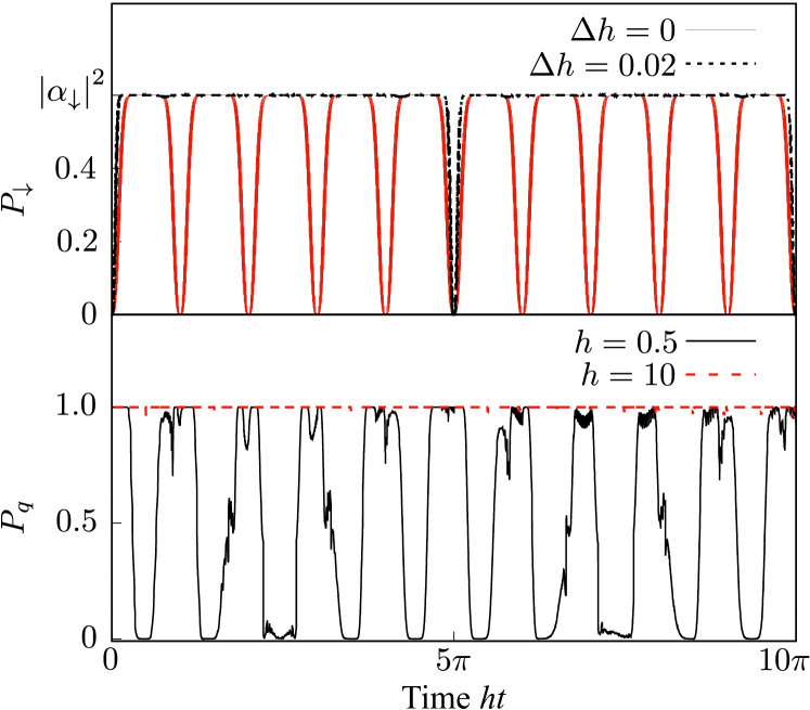
Figure 2: (Color online) The evolution of $P_{\downarrow}$ and $P_{q}$. The parameters are chosen as same as those in Fig. 1, except that $h_{j}$ is uniformly distributed in the range $[h,h+\Delta h)$, expressed as $h_{j}=h+\left(j-1\right)\Delta h/N$. For the top panel, we choose $h=0.01$. And for the bottom panel, we fix $\Delta h=0.02$.

The numerical results verify above analysis and show that the Born’s rule is stable against small perturbations. We notice that, in the stochastic dynamics, the wave-function does not evolve exactly into the classical states ($\ket{\uparrow}$ or $\ket{\downarrow}$) for a finite $N$, but can be infinitely close to them in the limit $N\to\infty$. The Born’s rule is only an approximation in the case of large $N$. For numerical calculation, we define the projection

$$u=\left|\braket{\uparrow}{\phi_{n^{\prime},n}(t)}\right|^{2}.$$ (12)

The projection has a distribution at a given time, denoted by $P(u)$ with $u\in[0,1]$. That $u$ is close to zero (one) means that the wave-function is in the classical state $\ket{\downarrow}$ ($\ket{\uparrow}$). And we define a small positive number $\epsilon$ (dubbed the error), which denotes how close to the classical states the wave-function is for being considered as classical. In this spirit, $P_{\downarrow}=P(0\leq u\leq\epsilon)$ is the probability of the system being in the state $\ket{\downarrow}$, $P_{\uparrow}=P(1-\epsilon\leq u\leq 1)$ is the probability of the system being in the state $\ket{\uparrow}$. And $P_{q}=1-P_{\uparrow}-P_{\downarrow}$ is the probability that the system is not in the classical states but has to be treated as the superposition of them, i.e., the classicality fails to emerge and the quantum superposition dominates.

Fig. 1 shows the evolution of $P_{\uparrow}$ and $P_{\downarrow}$ at different $N$. For a large $N$ ($N=80$), we see that the wave-function quickly collapses into the classical states with the probabilities obeying the Born’s rule ($P_{\uparrow/\downarrow}=\left|\alpha_{\uparrow/\downarrow}\right|^{2}$). The collapsing time decreases with $N$ increasing. The wave-function collapse and the Born’s rule have already been seen for $N=10$, but they are absent for a smaller $N$ ($N=2$). An interesting feature of Fig. 1 is the periodic resurrection of quantum superposition and suppression of collapse when the time is an integer times of $\pi/\omega^{\downarrow}$. This is not surprising. At these specific times, the spin-up and spin-down significances become similar to each other because $\sin\left(\omega^{\downarrow}t\right)=0$, thereafter, the superposition between classical states resurrects.

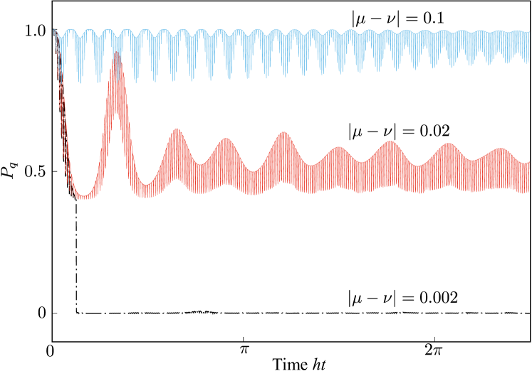
Figure 3: (Color online) The probability $P_{q}$ at different $\left|\mu-\nu\right|$. Here we choose $h=0.01$ and $\Delta h=0.02$.

The resurrection of quantum superposition can be suppressed by a dispersed $h_{j}$. The resurrection of superposition needs $\left|G^{\downarrow}_{j}\right|^{2}_{d_{j}=1}=1$ and $\left|G^{\downarrow}_{j}\right|^{2}_{d_{j}=-1}=0$. From Eq. (11), we see that this is satisfied only if $\omega_{j}^{\downarrow}t$ is an integer times of $\pi$. But the frequency $\omega_{j}$ depends on $h_{j}$. A dispersed $h_{j}$ results in a dispersed frequency, so that this condition is hard to be simultaneously satisfied for different $j$, and then the resurrection is avoided. Fig. 2 (top panel) compares $P_{\downarrow}(t)$ between a constant $h_{j}$ and a dispersed $h_{j}$. We see that a dispersed $h_{j}$ does suppress the resurrection by increasing its period by five times. The resurrection is still present since there are only finite number of frequencies ($N=10$). One expects that the resurrection will be further suppressed with $N$ increasing.

The bottom panel of Fig. 2 shows the probability of quantum superposition for different $h$. We see a strong coupling between system and environment in the vertical direction kills the classicality. The emergence of classicality ($P_{q}\approx 0$) can be seen sometimes at $h=0.5$, but is totally lost at $h=10$.

We have argued that one condition of wave-function collapse is $\left|\mu-\nu\right|/h\ll 1$. Fig. 3 compares $P_{q}$ for different $\left|\mu-\nu\right|$, while $h$ is fixed to $0.01$. The wave-function collapse and the Born’s rule are stable against a small $\left|\mu-\nu\right|$. At $\left|\mu-\nu\right|=0.002$, the wave-function collapse and the Born’s rule are still clear ($P_{q}=0$). But with $\left|\mu-\nu\right|$ increasing, the classicality gradually vanishes, and the quantum effect resurrects. When $\left|\mu-\nu\right|=0.1$ is ten times of $h$, the probability of wave-function collapsing completely vanishes.

6 Conclusions

In summary, our model of wave-function stochastic evolution succeeds in explaining the emergence of classicality and the Born’s rule for an open system. Our main assumptions are Eqs. (3) and (4), which give the trajectories of the wave-function and their corresponding probability. The randomness in the wave-function evolution is environment-induced, depending on the interaction between system and environment. And it vanishes with the interaction. For an isolated system, Eqs. (3) and (4) coincide exactly with the Schrödinger equation.

We study the stochastic dynamics in the central spin model, showing how it results in the wave-function collapse and the Born’s rule for the system-environment interaction in a specific range. The Born’s rule is then not a priori hypothesis any more, but an approximation in the large-environment limit. The condition for the emergence of classicality is $\left|\mu-\nu\right|/\left|h_{j}\right|\ll 1$, $\left|h_{j}\right|\ll 1$ and a dispersed $h_{j}$. If these conditions are not satisfied, e.g., in the case $h_{j}=0$ or $\nu=0$, the superposition between classical states is preserved in the evolution, and classicality does not emerge. Therefore, the quantum superposition is not limited in the microscopic world, and classicality is not always present in the macroscopic world. Whether the system keeps the quantum superposition or shows classicality is determined by how the system interacts with its environment. This is the spirit of einselection or quantum Darwinism. But in our theory, the loss of superposition is objective, with the process described explicitly by Eqs. (3) and (4).

Eqs. (3) and (4) give the random trajectory of the wave-function for an open system. While quantum mechanics predicts the reduced density for an open system. There is a one-to-many map between a reduced density matrix and the random distributions of wave-functions. According to Eq. (5), the random trajectory predicts exactly the same reduced density matrix as quantum mechanics. But quantum mechanics by itself cannot predict the random trajectory in an open system. This explains why we can derive the Born’s rule but it has to be an axiom in quantum mechanics.

It is worth emphasizing the difference between our approach and previous ones, especially the ones based on many-world interpretation or spontaneous collapse model. In the many-world interpretation, the evolution of the physical state of the universe is deterministic. The probability (the Born’s rule) has to be introduced into the theory by Zurek’s envariance or Deutsch’s decision theory. But in our theory, the evolution of the system’s wave function is defined to be stochastic with the probability explicitly given by Eq. (4). At this point, our theory is similar to the spontaneous collapse models which also assume stochastic evolution. But the spontaneous collapse models are expressed in terms of stochastic differential equations. The treatment of these equations and their generalization to relativistic model are difficult. While in our theory, the stochastic process is defined according to the Schrödinger equation (3) of orthodox quantum mechanics with which the physicists are familiar. The price we have to pay is that the Born’s rule in our theory becomes an approximation which stands only for some specific system-environment interaction.

Therefore, we propose a model of the wave-function objectively collapsing. It is falsifiable, because one can use it to judge which type of system-environment interaction can induce collapse and which cannot. Our model might be helpful in explaining the recent experiments on the wave-function collapse in mesoscopic systems.

- (1) D. Bohm, Phys. Rev. 85, 166 (1952).
- (2) H. Everett, Rev. Mod. Phys. 29, 454 (1957).
- (3) W. H. Zurek, Rev. Mod. Phys. 75, 715 (2003).
- (4) A. Bassi, K. Lochan, S. Satin, T. P. Singh, and H. Ulbricht, Rev. Mod. Phys. 85, 471 (2013).
- (5) M. A. Nielsen and I. L. Chuang, Quantum computation and quantum information (Cambridge University Press, Cambridge, 2000).
- (6) N. Bohr, Nature (London) 121, 580 (1928).
- (7) A. M. Gleason, J. Math. Mech. 6, 885 (1957).
- (8) H. D. Zeh, Found. Phys. 1, 69 (1970).
- (9) W. H. Zurek, Phys. Rev. D 24, 1516 (1981).
- (10) W. H. Zurek, Phys. Rev. D 26, 1862 (1982).
- (11) D. Deutsch, Proc. Roy. Soc. Lond. A 455, 3129 (1999).
- (12) H. Barnum, C. M. Caves, J. Finkelstein, C. A. Fuchs, and R. Schack, Proc. Roy. Soc. Lond. A 456, 1175 (2000).
- (13) S. Saunders, Proc. Roy. Soc. Lond. A 460, 1771 (2004).
- (14) D. Wallace, Stud. Hist. Philos. Sci. Part B 34, 415 (2003).
- (15) D. Wallace, Stud. Hist. Philos. Sci. Part B 38, 311 (2007).
- (16) W. H. Zurek, Phys. Rev. Lett. 90, 120404 (2003).
- (17) W. H. Zurek, Phys. Rev. A 71, 052105 (2005).
- (18) M. Schlosshauer and A. Fine, Found. Phys. 35, 197 (2005).
- (19) A. I. M. Rae, Stud. Hist. Philos. Sci. Part B 40, 243 (2009).
- (20) F. Herbut, Eur. Phys. J. Plus 127, 14 (2012).
- (21) A. L. G. Mandolesi, Found. Phys. 48, 751 (2018).
- (22) A. L. G. Mandolesi, Found. Phys. 49, 24 (2019).
- (23) A. L. G. Mandolesi, Phys. Lett. A 384, 126725 (2020).
- (24) G. ’t Hooft, arXiv:1112.1811.
- (25) M. Genovese, Physics Reports 413, 319 (2005).
- (26) D. Bohm, Phys. Rev. 85, 166 (1952).
- (27) D. Bohm, Phys. Rev. 85, 180 (1952).
- (28) M. D. Towler, N. J. Russell, and A. Valentini, Proc. Roy. Soc. Lond. A 468, 990 (2012).
- (29) A. Khrennikov, J. Phys. A: Math. Gen. 38, 9051 (2005).
- (30) G. C. Ghirardi, A. Rimini, and T. Weber, Phys. Rev. D 34, 470 (1986).
- (31) A. Bassi, J. Phys. A 38, 3173 (2005).
- (32) P. Pearle, Phys. Rev. A 39, 2277 (1989).
- (33) G. C. Ghirardi, P. Pearle, and A. Rimini, Phys. Rev. A 42, 78 (1990).
- (34) M. Arndt and K. Hornberger, Nature Physics 10, 271 (2014).
- (35) A. Pontin, N. P. Bullier, M. Toroš, and P. F. Barker, arXiv:1907.06046 (2019).
- (36) Z.-Q. Yin, T. Li, X. Zhang, and L. M. Duan, Phys. Rev. A 88, 033614 (2013).
- (37) M. Bahrami, M. Paternostro, A. Bassi, and H. Ulbricht, Phys. Rev. Lett. 112, 210404 (2014).
- (38) S. Nimmrichter, K. Hornberger, and K. Hammerer, Phys. Rev. Lett. 113, 020405 (2014).
- (39) L. Diósi, Phys. Rev. Lett. 114, 050403 (2015).
- (40) D. Goldwater, M. Paternostro, and P. F. Barker, Phys. Rev. A 94, 010104 (2016).
- (41) C. Jones, T. Guaita, and A. Bassi, arXiv:1907.02370 (2019).
- (42) K. Kraus, Found. Phys. 11, 547 (1981).
- (43) K. Kraus, Found. Phys. 15, 717 (1985).
- (44) M. A. Braun and K. Urbanowski, Physica A 190, 130 (1992).
- (45) K. Urbanowski, Found. Phys. Lett. 6, 167 (1993).
- (46) T. A. Brun, Am. J. Phys. 70, 719 (2002).
- (47) K. Jacobs and D. A. Steck, Contemp. Phys. 47, 279 (2006).
- (48) A. Patel and P. Kumar, Phys. Rev. A 96, 022108 (2017).
- (49) A. V. Ilyin, Found. Phys. 46, 845 (2016).
- (50) T. D. Galley and L. Masanes, Quantum 1, 15 (2017).
- (51) T. D. Galley and L. Masanes, Quantum 2, 104 (2018).
- (52) R. Sorkin, Mod. Phys. Lett. A 9, 3119 (1994).
- (53) U. Sinha, C. Couteau, T. Jennewein, R. Laflamme, and G. Weihs, Science 329, 418 (2010).
- (54) J. Q. Quach, Phys. Rev. A 95, 042129 (2017).
- (55) M.-O. Pleinert, J. von Zanthier, and E. Lutz, Phys. Rev. Research 2, 012051(R) (2020).
- (56) M. Zwolak, C. J. Riedel, and W. H. Zurek, Scientific Reports 6, 25277 (2016).