Simple smoothness indicator WENO-Z scheme for hyperbolic conservation laws

Abstract

The advantage of WENO-JS5 scheme [ J. Comput. Phys. 1996] over the WENO-LOC scheme [J. Comput. Phys.1994] is that the WENO-LOC nonlinear weights do not achieve the desired order of convergence in smooth monotone regions and at critical points. In this article, this drawback is achieved with the WENO-LOC smoothness indicators by constructing a WENO-Z type nonlinear weights which contains a novel global smoothness indicator. This novel smoothness indicator measures the derivatives of the reconstructed flux in a global stencil, as a result, the proposed numerical scheme could decrease the dissipation near the discontinuous regions. The theoretical and numerical experiments to achieve the required order of convergence in smooth monotone regions, at critical points, the essentially non-oscillatory (ENO), the analysis of parameters involved in the nonlinear weights like $\epsilon$ and $p$ are studied. From this study, we conclude that the imposition of certain conditions on $\epsilon$ and $p$, the proposed scheme achieves the global order of accuracy in the presence of an arbitrary number of critical points. Numerical tests for scalar, one and two-dimensional system of Euler equations are presented to show the effective performance of the proposed numerical scheme.

Keywords— Hyperbolic conservation laws, WENO scheme, discontinuity, smoothness indicators, non-linear weights, Runge-Kutta schemes.
MSC Subject Classification— 65M20, 65N06, 41A10.

1 Introduction

The study of hyperbolic conservation laws

$$\frac{\partial\mathbf{u}}{\partial t}+\frac{\partial f(\mathbf{u})}{\partial x} =0,\mathbf{x}\in\mathbb{R}^{d},(d\geq 1),t>0,$$ (1.1)

$$\mathbf{u}(x,0) =\mathbf{u}_{0}(x),\mathbf{x}\in\mathbb{R}^{d},$$

is one of the important topics in the areas of gas dynamics, shallow water flows and magneto-hydro-dynamics(MHD). For the equation (1.1), $\mathbf{u}=(u_{1},u_{2},......,u_{m})^{T}$ represents a conserved quantity which is a $m$-dimensional vector and flux $f(\mathbf{u})$, is a vector-valued function of $m$ components, $x$ and $t$ denote the space and time variables respectively. It is well known that the analytical solutions are available only for a few model problems and thus, numerical techniques play a important role in solving problems of practical interest. The vital remark in the solutions of hyperbolic conservation laws is that even if the smooth initial data may give rise to discontinuities as the time is propagating. For resolving this scenario and to obtain a valid solution, many numerical techniques such as finite difference, finite volume and finite element techniques have been developed.
Among them, the essentially non-oscillatory(ENO) schemes [1, 2, 3, 4] and the weighted essentially non-oscillatory (WENO) schemes [5, 6] are quite popular. As our interest is on WENO schemes, we briefly mention the details about these schemes. The WENO schemes first developed in $1994$ by Liu, Osher, and Chan [5] in a finite-volume framework where the authors came up with an ingenious idea as such: instead of choosing the smoothest candidate stencil, a nonlinear convex combination of all the sub stencils is used which results overall, a high-order accurate scheme when it is compared to ENO schemes. The major contributions of this technique are the construction of the nonlinear weights and the smoothness indicators based on undivided differences. Later in $1996$ [6], a finite difference WENO schemes are developed with the construction of new smoothness indicators, commonly known as WENO-JS (JS stands for Jiang & Shu) schemes. Hereafter, we refer the finite difference WENO formulation with the smoothness indicators of [5] as WENO-LOC scheme. The smoothness indicators of the WENO-JS scheme are the square sum of all the derivatives of $m$ local interpolating polynomials, the process leads to obtaining $(2m-1)^{th}-$order accuracy of the scheme in smooth regions. These schemes are extended by Balsara and Shu in [7] to a WENO family up to $11^{th}-$order accuracy. Besides, Gerolymous et al. [8] introduced a WENO family up to $17^{th}-$order. Balsara et al. [9] analyzed the WENO scheme presented in [7] in a basis set formed by Legendre polynomials up to $9^{th}-$order which affords an equivalent formulation for the numerical fluxes, as a result, the smoothness indicators are in the compact form. And further, the smoothness indicators have been written as the sum of perfect squares which makes the method more efficient and also more accurate for certain benchmark problems. This procedure further carried out in [10] up to $17^{th}-$order. Henrick et al. [11] studied the WENO-JS scheme and discovered that the WENO-JS nonlinear weights failed to recover the optimal order of accuracy at the critical points where the first-order derivative vanish but not the third-order derivative and observed that the scheme is sensitive with respect to the choice of $\epsilon$, the parameter used in the evaluation of nonlinear weights. To dissolve this issue and to achieve the required order of accuracy in presence of critical points, the authors altered the nonlinear weights through the construction of a mapping function which approximates the WENO convex combination intently to the optimal weights except at highly non-smooth regions. Another approach was adapted by Borges et al. [12] where the author’s designed global smoothness measurements for the fifth-order WENO scheme, dubbed as WENO-Z, which has the same accuracy as that of mapped WENO with the lower computational cost. Castro et al. [13] extended WENO-Z schemes to the higher-order, which have computationally cheaper nonlinear weights than mapped WENO through the construction of high-order smoothness indicators that can be obtained from the inexpensive linear combination of existing lower order smoothness indicators. Many modified and improved versions of the WENO schemes can be seen [14, 15, 16, 17, 19, 20, 21, 22, 23, 24, 25, 26, 34].

It is well known that the WENO schemes are quite popular from last two decades to approximate the solutions of the hyperbolic conservation laws through the smoothness indicators developed in [6], the authors, Jiang and Shu, modified the smoothness indicators developed in [5] as in smooth monotone regions and at the critical points the WENO-LOC scheme does not achieve the desired order of accuracy. To resolve this, in this paper, we have constructed a WENO-Z type nonlinear weights with WENO-LOC smoothness indicators. A novel global smoothness indicator is devised by measuring the derivatives of the reconstructed flux through undivided differences, as a result, the numerical scheme could decrease the dissipation around the discontinuities. Further, the proposed numerical scheme achieves the sufficient condition and ENO property to gain the required order of accuracy in smooth regions and at critical points. Several benchmark problems in the scalar, the system of one- and two-dimensional Euler equations are performed to show the effective performance of the proposed numerical scheme. It is shown that the proposed WENO scheme provides improved behavior to the fifth-order WENO-LOC and fifth-order WENO-JS (WENO-JS5) schemes. Furthermore, the consistency analysis of the numerical scheme is developed and shown that the imposition of certain conditions on the weight parameters leads to achieve the desired global order of accuracy in the presence of the arbitrary number of critical points.

The rest of the paper is organized as follows. The detailed formulation of the WENO scheme with the WENO-LOC and WENO-JS5 schemes are given in Section 2. In Section 3, the design of new nonlinear weights is proposed and performed the ENO property, accuracy test in smooth regions, near discontinuities and at critical points. Numerics have been performed for some benchmark problems like a scalar, one and two-dimensional Euler equations in Section 4. Concluding remarks are given in Section 5.

2 Numerical Scheme

In this section, for completeness we report the flux version of fifth-order WENO schemes presented in [6] for hyperbolic conservation laws (1.1).

2.1 WENO schemes

Let $\{I_{i}\}_{i}$ with $I_{i}=[x_{i-\frac{1}{2}},x_{i+\frac{1}{2}})$ be the partition of computational domain in space and let $x_{i}=\frac{1}{2}(x_{i+\frac{1}{2}}+x_{i-\frac{1}{2}})$ denote the center of the cell $I_{i}$ with the uniform cell length $\Delta x=x_{i+\frac{1}{2}}-x_{i-\frac{1}{2}}$. The function value $f$ at the node $x_{i}$ is given by $f_{i}:=f(x_{i}).$ Moreover, we use the notation $u_{i}^{n}$ for the approximation to $u$ at the grid point $(x_{i},t^{n})$ and $t^{n}=n\Delta t$. For simplicity, we restrict our discussion to one-dimensional scalar formulation of (1.1),

$$u_{t}=-f(u)_{x},$$ (2.1)

and the associated semi-discretized formulation is

$$\frac{d{u_{i}(t)}}{dt}=-\frac{1}{\Delta x}\left({\hat{f}_{i+\frac{1}{2}}-\hat{f}_{i-\frac{1}{2}}}\right)=:L(u),$$ (2.2)

where $u_{i}(t)$ is the numerical approximation to the point value $u(x_{i},.)$ and the numerical flux $\hat{f}$ is a function of $(r+s)$ arguments i.e., $\hat{f}_{i+\frac{1}{2}}=\hat{f}(u_{i-r},...,u_{i+s}).$ The system of ODE’s (2.2) can be obtained by using the strong-stablity preserving Runge-Kutta methods [27].

The numerical flux function $\hat{f}$ in (2.2) should be consistent with the physical flux $f,$ that is, $\hat{f}(u,...,u)=f(u)$ and should satisfy the Lipschitz continuity in each of its arguments, as a requirement for the applicability of Lax-Wendroff theorem [28].

To compute the numerical flux $\hat{f}_{i\pm\frac{1}{2}},$ a function $h$ is defined implicitly (see Lemma 2.1 of [4])

$$f(x):=f(u(x,.))=\frac{1}{\Delta x}\int_{x-\frac{\Delta x}{2}}^{x+\frac{\Delta x}{2}}h(\xi)d\xi.$$ (2.3)

The differentiation of equation (2.3) and evaluation at the point $x=x_{i}$ yields

$$\frac{\partial f}{\partial x}\bigg{|}_{x=x_{i}}=\frac{1}{\Delta x}\left(h_{i+\frac{1}{2}}-h_{i-\frac{1}{2}}\right),$$ (2.4)

which indicates that the numerical flux $\hat{f}$ approximates $h$ at cell boundaries $x_{i\pm\frac{1}{2}}$ with high-order of accuracy, that is,

$$\hat{f}_{i\pm\frac{1}{2}}=h(x_{i\pm\frac{1}{2}})+O\big{(}\Delta x^{k}\big{)},$$

where $k$ depending on the degree of interpolation. The basic observation reveals that the spatial derivative defined in (2.1) is exactly approximated by a conservative finite difference formula (2.4) at the cell boundaries. Using equation (2.4) in equation (2.2), we have

$$\frac{du_{i}(t)}{dt}=-\frac{1}{\Delta x}\left(h_{i+\frac{1}{2}}-h_{i-\frac{1}{2}}\right)\approx-\frac{1}{\Delta x}\left(\hat{f}_{i+\frac{1}{2}}-\hat{f}_{i-\frac{1}{2}}\right).$$ (2.5)

In order to ensure the numerical stability, the flux $f(u)$ is splitted into two parts $f^{+}$ and $f^{-}$ such that

$$f(u)=f^{+}(u)+f^{-}(u),$$ (2.6)

where $\frac{df^{+}(u)}{du}\geq 0$ and $\frac{df^{-}(u)}{du}\leq 0.$ Among many flux splitting methods, we use global Lax-Friedrichs splitting

$$f^{\pm}(u)=\frac{1}{2}(f(u)\pm\alpha u),$$ (2.7)

where $\alpha=\displaystyle\max_{u}|f{{}^{\prime}}(u)|$ for its simplicity and capability to produce very smooth fluxes. Let $\hat{f}^{+}_{i+\frac{1}{2}}$ and $\hat{f}^{-}_{i+\frac{1}{2}}$ be the numerical fluxes obtained from the positive and negative parts of $f(u)$ respectively and from (2.6), we have

$$\hat{f}_{i+\frac{1}{2}}=\hat{f}_{i+\frac{1}{2}}^{+}+\hat{f}_{i+\frac{1}{2}}^{-}.$$ (2.8)

Now we describe only how $\hat{f}_{i+\frac{1}{2}}^{+}$ can be approximated since $\hat{f}_{i+\frac{1}{2}}^{-}$ is symmetric to the positive part with respect to $x_{i+\frac{1}{2}}.$ In the formulation of $\hat{f}_{i+\frac{1}{2}}^{+}$, for simplicity, we drop the ${}^{`}+^{`}$ sign in the superscript.

Choose a larger stencil $T=\{I_{i-r},...,I_{i+r}\}$. Consider a fourth degree polynomial($r=2$) based on the nodal point information of the numerical flux which satisfies

$$\frac{1}{\Delta x}\int_{I_{j}}p(\xi)d\xi=\frac{1}{\Delta x}\int_{I_{j}}h(\xi)d\xi=f_{j},j=i-r,...,i+r.$$ (2.9)

Evaluating this polynomial $p(x)$ at $x=x_{i+\frac{1}{2}}$ gives

$$\hat{f}_{i+\frac{1}{2}}:=P(x_{i+\frac{1}{2}})=\frac{1}{60}(2f_{i-2}-13f_{i-1}+47f_{i}+27f_{i+1}-3f_{i+2}).$$ (2.10)

If there is a discontinuity inside the stencil $T$, then the corresponding interpolation process to the approximation of flux $\hat{f}_{i+\frac{1}{2}}$ may generate oscillations. In order to alleviate this the WENO procedure is employed, in which the stencil $T$ is divided into $(r+1)$ smaller stencils: $S_{k}=\{I_{i-r+k},...,I_{i+k}\},k=0,...,r$. The second degree polynomials $p^{k}(x),k=0,...,r$ are constructed in the associated stencils $S_{k}$ to approximate the function $h(x)$ that satisfies

$$\frac{1}{\Delta x}\int_{I_{j}}p^{k}(\xi)d\xi=\frac{1}{\Delta x}\int_{I_{j}}h(\xi)d\xi=f_{j},j=i-r+k,...,i+k;k=0,...,r.$$

The explicit expressions of polynomials $p^{k}(x),k=0,1,2$ as

$$p^{0}(x)= \frac{1}{24}\left[(-f_{i-2}+2f_{i-1}+23f_{i})+12(f_{i-2}-4f_{i-1}+3f_{i})\eta+12(f_{i-2}-2f_{i-1}+f_{i})\eta^{2}\right],$$

$$p^{1}(x)= \frac{1}{24}\left[(-f_{i-1}+26f_{i-1}-f_{i+1})+12(f_{i+1}-f_{i-1})\eta+12(f_{i-1}-2f_{i}+f_{i+1})\eta^{2}\right],$$

$$p^{2}(x)= \frac{1}{24}\left[(23f_{i}+2f_{i+1}-f_{i+2})+12(-3f_{i}+4f_{i+1}-f_{i+2})\eta+12(f_{i}-2f_{i+1}+f_{i+2})\eta^{2}\right],$$

where $\eta=\left(\frac{x-x_{i}}{\Delta x}\right)$. The evaluation of these polynomials $p^{k}(x),k=0,1,2$ at $x=x_{i+\frac{1}{2}}$ gives

$$\begin{aligned} \hat{f}_{i+\frac{1}{2}}^{0}=&\frac{1}{6}(2f_{i-2}-7f_{i-1}+11f_{i}),\\ \hat{f}_{i+\frac{1}{2}}^{1}=&\frac{1}{6}(-f_{i-1}+5f_{i}+2f_{i+1}),\\ \hat{f}_{i+\frac{1}{2}}^{2}=&\frac{1}{6}(2f_{i}+5f_{i+1}-f_{i+2}).\end{aligned}$$ (2.11)

The Taylor’s expansion of (2.11) reveals

$$\hat{f}_{i+\frac{1}{2}}^{0} = h_{i+\frac{1}{2}}-\frac{\Delta x^{3}}{4}f{}^{(3)}(0)+O\left(\Delta x^{4}\right),$$

$$\hat{f}_{i+\frac{1}{2}}^{1} = h_{i+\frac{1}{2}}+\frac{\Delta x^{3}}{12}f{}^{(3)}(0)+O\left(\Delta x^{4}\right),$$

$$\hat{f}_{i+\frac{1}{2}}^{2} = h_{i+\frac{1}{2}}-\frac{\Delta x^{3}}{12}f{}^{(3)}(0)+O\left(\Delta x^{4}\right).$$

The values of the function $p(x)$ at the point $x=x_{i+\frac{1}{2}}$ of cell $I_{i}$, can be written as a linear combination of $p^{k}(x)$ at the point $x=x_{i+\frac{1}{2}}$ in the smooth regions. Thus the linear/ideal weights are defined as

$$\hat{f}_{i+\frac{1}{2}}=\sum_{k=0}^{2}d_{k}\hat{f}^{k}_{i+\frac{1}{2}}.$$ (2.12)

The values of these linear weights are $d_{0}=\frac{1}{10}$, $d_{1}=\frac{3}{5}$, $d_{2}=\frac{3}{10}$. Note that each $d_{k}\geq 0$ and $\displaystyle\sum_{k=0}^{2}d_{k}=1.$

In the non-smooth regions, (2.12) is not valid to approximate the flux function $\hat{f}_{i+\frac{1}{2}}$ in terms of local information. This issue is resolved by introducing the nonlinear weights $\omega_{k}$ such that

$$\hat{f}_{i+\frac{1}{2}}=\sum_{k=0}^{2}\omega_{k}\hat{f}^{k}_{i+\frac{1}{2}}.$$ (2.13)

These nonlinear weights constructed in subsequent steps are such that in smooth regions, the nonlinear weights should converge to the linear weights with the required order of accuracy and in the non-smooth regions, these have to tend to zero so that the contribution from the non-smooth regions to the approximation of the flux $\hat{f}_{i+\frac{1}{2}}$ is negligible, with this the final reconstruction is essentially non-oscillatory. Thus, the nonlinear weights have to satisfy the following properties:
Convexity:

$$\sum_{k=0}^{2}\omega_{k}=1,\omega_{k}\geq 0,k=0,1,2.$$ (2.14)

Optimal Order: If $f$ is smooth in stencil $T$, then

$$L(u)=f^{\prime}(x_{i})+O\bigg{(}\Delta x^{5}\bigg{)}.$$ (2.15)

ENO property: If a substencil $T^{D}\subset T$ contains a discontinuity of $f$, but there exists another sub-stencil $T^{C}\subset T$ where $f$ is smooth, then

$$\begin{aligned} \omega_{D}&=O(\Delta x^{q})\text{ {for\,some} }q>0,\text{and}\\ \omega_{C}&=\varTheta(1),\end{aligned}$$

as $\Delta x\rightarrow 0,$ where $O(\cdot)$ and $\varTheta(\cdot)$ are standard Bachmann-Landau notation [29].

The following result relate the effective order of accuracy of a WENO scheme to the difference between its non-linear weights $\omega_{k}$ and the linear weights $d_{k}.$

Lemma 2.1.

(Sufficient Condition) If the nonlinear weights satisfy the condition

$$\begin{cases}\omega_{k}-d_{k}&=O(\Delta x^{2}),\\ \omega_{k}^{+}-\omega_{k}^{-}&=O(\Delta x^{3}),\end{cases}k=0,1,2,$$ (2.16)

or

$$\omega_{k}-d_{k}=O(\Delta x^{3}),k=0,1,2,$$ (2.17)

then the corresponding WENO scheme satisfy the optimal order of accuracy, where the superscripts ${}^{\prime}+^{\prime}$ or ${}^{\prime}-^{\prime}$ on $\omega_{k}$ correspond to their use in $\hat{f}_{i+\frac{1}{2}}$ or $\hat{f}_{i-\frac{1}{2}}$ respectively [11, 12].

2.2 WENO-LOC weights and its order of convergence

The nonlinear weights defined in [5] are

$$\omega_{k}=\frac{\alpha_{k}}{\displaystyle\sum_{l=0}^{2}\alpha_{l}},\,\alpha_{k}=\frac{d_{k}}{\left(\epsilon+\beta_{k}\right)^{p}},$$ (2.18)

where $\epsilon$ is a small positive number which is set to be $\epsilon=10^{-5}$ to avoid division by zero, $p=2$ is chosen to increase the difference of scales of distinct weights at non-smooth parts of the solution. Note that $\alpha_{k}$ are the unnormalized weights and $\omega_{k}$ are the normalized weights. The smoothness of the flux is measured by the derivatives of the reconstructed flux $\hat{f}_{i+\frac{1}{2}}^{k}$ on each stencil $S_{k}$, $k=0,1,2,$ based on the undivided differences as

$$\beta_{k}=\sum_{n=1}^{2}\sum_{m=1}^{3-n}\frac{(f[i+k+m-3,n])^{2}}{3-n},k=0,1,2,$$ (2.19)

where $f[\cdot,\cdot]$ is the $n^{\text{th}}$ undivided difference,

$$f[i,0] = f_{i},$$

$$f[i,n] = f[i+1,n-1]-f[i,n-1].$$

So, we have

$$\beta_{k}=\frac{1}{2}\left((f{[i+k-2,1]})^{2}+(f{[i+k-1,1]})^{2})\right)+(f{[i+k-2,2]})^{2},k=0,1,2,$$ (2.20)

and its explicit form for $k=0,1,2$ are

$$\begin{aligned} \beta_{0}&=\frac{1}{2}\left((f_{i-1}-f_{i-2})^{2}+(f_{i}-f_{i-1})^{2})\right)+(f_{i}-2f_{i-1}+f_{i-2})^{2},\\ \beta_{1}&=\frac{1}{2}\left((f_{i}-f_{i-1})^{2}+(f_{i+1}-f_{i})^{2})\right)+(f_{i-1}-2f_{i}+f_{i+1})^{2},\\ \beta_{2}&=\frac{1}{2}\left((f_{i+1}-f_{i})^{2}+(f_{i+2}-f_{i+1})^{2})\right)+(f_{i+2}-2f_{i+1}+f_{i})^{2}.\end{aligned}$$ (2.21)

The Taylor’s expansion of the smoothness indicator (2.21) of the candidate stencils at $x=x_{i}$ are expressed as

$$\beta_{0} =\left(f_{i}^{\prime}\right)^{2}\Delta x^{2}-2f_{i}^{\prime}f_{i}^{\prime\prime}\Delta x^{3}+\left(\frac{4}{3}f_{i}^{\prime}f_{i}^{\prime\prime\prime}+\frac{9}{4}\left(f_{i}^{\prime\prime}\right)^{2}\right)\Delta x^{4}-\frac{23}{6}f_{i}^{\prime\prime}f_{i}^{\prime\prime\prime}\Delta x^{5}+O(\Delta x^{6}),$$

$$\beta_{1} =\left(f_{i}^{\prime}\right)^{2}\Delta x^{2}+\left(\frac{1}{3}f_{i}^{\prime}f_{i}^{\prime\prime\prime}+\frac{5}{4}\left(f_{i}^{\prime\prime}\right)^{2}\right)\Delta x^{4}+O(\Delta x^{6}),$$ (2.22)

$$\beta_{2} =\left(f_{i}^{\prime}\right)^{2}\Delta x^{2}+2f_{i}^{\prime}f_{i}^{\prime\prime}\Delta x^{3}+\left(\frac{4}{3}f_{i}^{\prime}f_{i}^{\prime\prime\prime}+\frac{9}{4}\left(f_{i}^{\prime\prime}\right)^{2}\right)\Delta x^{4}+\frac{23}{6}f_{i}^{\prime\prime}f_{i}^{\prime\prime\prime}\Delta x^{5}+O(\Delta x^{6}),$$

Substituting (2.22) into (2.18), we get

$$\alpha_{0} = \frac{1}{10\left(f_{i}^{\prime}\right)^{4}\Delta x^{4}}\left(1+4\frac{f_{i}^{\prime\prime}}{f_{i}^{\prime}}\Delta x-\left(\frac{8}{3}\frac{f_{i}^{\prime\prime\prime}}{f_{i}^{\prime}}+\frac{9}{2}\frac{\left(f_{i}^{\prime\prime}\right)^{2}}{\left(f_{i}^{\prime}\right)^{2}}\right)\Delta x^{2}+O(\Delta x^{3})\right),$$

$$\alpha_{1} = \frac{6}{10\left(f_{i}^{\prime}\right)^{4}\Delta x^{4}}\left(1-\left(\frac{2}{3}\frac{f_{i}^{\prime\prime\prime}}{f_{i}^{\prime}}+\frac{5}{2}\frac{\left(f_{i}^{\prime\prime}\right)^{2}}{\left(f_{i}^{\prime}\right)^{2}}\right)\Delta x^{2}+O(\Delta x^{3})\right),$$

$$\alpha_{2} = \frac{3}{10\left(f_{i}^{\prime}\right)^{4}\Delta x^{4}}\left(1-4\frac{f_{i}^{\prime\prime}}{f_{i}^{\prime}}\Delta x-\left(\frac{8}{3}\frac{f_{i}^{\prime\prime\prime}}{f_{i}^{\prime}}+\frac{9}{2}\frac{\left(f_{i}^{\prime\prime}\right)^{2}}{\left(f_{i}^{\prime}\right)^{2}}\right)\Delta x^{2}+O(\Delta x^{3})\right),$$

and

$$\omega_{0} = \frac{1}{10}+\frac{2f_{i}^{\prime\prime}}{5f_{i}^{\prime}}\Delta x+O(\Delta x^{2}),$$

$$\omega_{1} = \frac{6}{10}+O(\Delta x^{4}),$$ (2.23)

$$\omega_{2} = \frac{3}{10}-\frac{6f_{i}^{\prime\prime}}{5f_{i}^{\prime}}\Delta x+O(\Delta x^{2}).$$

Note that in the above procedure a small parameter $\epsilon$ is omitted since it is only used to avoid the denominator to be zero. From (2.23), it is concluded that the nonlinear weights approaches to the linear weights with first order of accuracy. So, the numerical scheme with WENO-LOC weights provides the overall fourth order of accuracy in smooth regions and further the order of accuracy degrades to third-order in presence of first-order critical points(which can observed by doing similar analysis on the unnormalized and normalized weights).

2.3 WENO-JS weights and its order of convergence

As observed in above, the smoothness indicators of WENO-LOC scheme does not achieve the optimal order of convergence in the smooth regions, the authors Jiang and Shu in [6] constructed a new smoothness measurements $\beta_{k}$ in (2.18) based on the concept of reducing the total variation of the numerical solution on each stencil as,

$$\beta_{k}=\sum_{l=1}^{2}\Delta x^{2l-1}\intop_{x_{i-\frac{1}{2}}}^{x_{i+\frac{1}{2}}}\left(\frac{d^{l}\hat{f}^{k}}{dx^{q}}\right)^{2}dx,$$ (2.24)

which is a scaled square sum of all the derivatives of interpolation polynomial $\hat{f}^{k}(x)$ over the interval $\left(x_{i-\frac{1}{2}},x_{i+\frac{1}{2}}\right)$. The explicit form of these smoothness indicators are as follows

$$\beta_{0} = \frac{13}{12}(f_{i-2}-2f_{i-1}+f_{i})^{2}+\frac{1}{4}(f_{i-2}-4f_{i-1}+3f_{i})^{2},$$

$$\beta_{1} = \frac{13}{12}(f_{i-1}-2f_{i}+f_{i+1})^{2}+\frac{1}{4}(f_{i+1}-f_{i-1})^{2},$$ (2.25)

$$\beta_{2} = \frac{13}{12}(f_{i}-2f_{i+1}+f_{i+2})^{2}+\frac{1}{4}(3f_{i}-4f_{i+1}+f_{i+2})^{2}.$$

By Taylor’s expansion of these smoothness indicators, one can obtain

$$\beta_{0} =\left(f_{i}^{\prime}\right)^{2}\Delta x^{2}+\left(\frac{13}{12}\left(f_{i}^{\prime\prime}\right)^{2}-\frac{2}{3}f_{i}^{\prime}f_{i}^{\prime\prime\prime}\right)\Delta x^{4}+\left(\frac{-13}{6}f_{i}^{\prime\prime}f_{i}^{\prime\prime\prime}+\frac{1}{2}f_{i}^{\prime}f_{i}^{iv}\right)\Delta x^{5}+O(\Delta x^{6}),$$

$$\beta_{1} =\left(f_{i}^{\prime}\right)^{2}\Delta x^{2}+\left(\frac{13}{12}\left(f_{i}^{\prime\prime}\right)^{2}+\frac{1}{3}f_{i}^{\prime}f_{i}^{\prime\prime\prime}\right)\Delta x^{4}+O(\Delta x^{6}),$$ (2.26)

$$\beta_{2} =\left(f_{i}^{\prime}\right)^{2}\Delta x^{2}+\left(\frac{13}{12}\left(f_{i}^{\prime\prime}\right)^{2}-\frac{2}{3}f_{i}^{\prime}f_{i}^{\prime\prime\prime}\right)\Delta x^{4}+\left(\frac{13}{6}f_{i}^{\prime\prime}f^{\prime\prime\prime}-\frac{1}{2}f_{i}^{\prime}f_{i}^{iv}\right)\Delta x^{5}+O(\Delta x^{6}).$$

Now, let us see the order of convergence of the nonlinear weights of WENO-JS5 scheme. Substituting (2.26) into (2.18) with $p=2$ and $\epsilon=0$, we get

$$\alpha_{0} = \frac{1}{\left(f_{i}^{\prime}\right)^{4}\Delta x^{4}}\left(\frac{1}{10}-\left(\frac{-2}{15}\frac{f_{i}^{\prime\prime\prime}}{f_{i}^{\prime}}+\frac{13}{60}\frac{\left(f_{i}^{\prime\prime}\right)^{2}}{\left(f_{i}^{\prime}\right)^{2}}\right)\Delta x^{2}+O(\Delta x^{3})\right),$$

$$\alpha_{1} = \frac{1}{\left(f_{i}^{\prime}\right)^{4}\Delta x^{4}}\left(\frac{6}{10}-\left(\frac{2}{5}\frac{f_{i}^{\prime\prime\prime}}{f_{i}^{\prime}}+\frac{13}{10}\frac{\left(f_{i}^{\prime\prime}\right)^{2}}{\left(f_{i}^{\prime}\right)^{2}}\right)\Delta x^{2}+O(\Delta x^{3})\right),$$

$$\alpha_{2} = \frac{1}{\left(f_{i}^{\prime}\right)^{4}\Delta x^{4}}\left(\frac{3}{10}-\left(\frac{-2}{5}\frac{f_{i}^{\prime\prime\prime}}{f_{i}^{\prime}}+\frac{13}{20}\frac{\left(f_{i}^{\prime\prime}\right)^{2}}{\left(f_{i}^{\prime}\right)^{2}}\right)\Delta x^{2}+O(\Delta x^{3})\right),$$

and

$$\omega_{0} = \frac{1}{10}+\frac{3f_{i}^{\prime\prime}}{25f_{i}^{\prime}}\Delta x^{2}+O(\Delta x^{3}),$$

$$\omega_{1} = \frac{6}{10}-\frac{12f_{i}^{\prime\prime}}{25f_{i}^{\prime}}\Delta x^{2}+O(\Delta x^{3}),$$ (2.27)

$$\omega_{2} = \frac{3}{10}+\frac{9f_{i}^{\prime\prime}}{25f_{i}^{\prime}}\Delta x^{2}+O(\Delta x^{3}).$$

From (2.27), we conclude that the WENO-JS5 nonlinear weights converges to the ideal weights with the second-order of accuracy. So, the numerical scheme with WENO-JS5 weights provides the overall fifth order of accuracy in smooth regions. Note that the advantage with the WENO-JS5 weights over the WENO-LOC weights is that it improves the one order of accuracy in smooth regions. Further the order of accuracy of WENO-JS5 scheme degrades to third-order in presence of first-order critical points and to second-order if the second derivatives vanishes.

3 Construction of a new nonlinear weights

A novel global smoothness measurement is constructed based on the linear combination of undivided differences of second-order derivatives which leads to provide a sixth-order of accuracy on the global stencil $S^{5}$ as

$$\begin{aligned} \zeta=\bigg{|}\left(\left(f_{i-2}-2f_{i-1}+f_{i}\right)^{2}-2\left(f_{i-1}-2f_{i}+f_{i+1}\right)^{2}+\left(f_{i}-2f_{i+1}+f_{i+2}\right)^{2}\right)\bigg{|},\end{aligned}$$

and the Taylor’s expansion of $\zeta$ gives

$$\zeta=2\bigg{|}\left(f_{i}{{}^{\prime\prime}}f_{i}^{(4)}+(f_{i}{{}^{\prime\prime\prime}})^{2}\right)\bigg{|}\Delta x^{6}+O(\Delta x^{8}).$$

Note that in the construction of WENO-LOC weights, the usage of the first-order derivatives in the smoothness indicators are not able to produce the required order of accuracy i.e., third-order, because of this reason, we avoid the first-order derivatives information in the construction of global smoothness measurement of the global stencil. Now, we define the nonlinear weights $\omega_{k}$ as

$$\omega_{k}=\frac{\alpha_{k}}{\displaystyle\sum_{k=0}^{2}\alpha_{k}},k=0,1,2,$$ (3.1)

and the unnormalized weights as

$$\alpha_{k}=d_{k}\left(1+\dfrac{\zeta}{\beta_{k}+\epsilon}\right),\;k=0,1,2,$$ (3.2)

such that the nonlinear weights $\omega_{k}$ converge to the ideal weights with the higher order of accuracy where we use (2.21) the smoothness indicators $\beta_{k}$. The parameter $\epsilon$ is taken as a small number to avoid the division by zero and chosen this value as $10^{-16}$.

Now, we check the convergence order of nonlinear weights in smooth regions i.e., $f_{i}^{\prime}\neq 0$. Substituting (2.22) into (3.2), we have

$$\alpha_{0} = \frac{1}{10}+\frac{1}{5}\left(\frac{f_{i}^{\prime\prime}f_{i}^{iv}}{\left(f_{i}^{\prime}\right)^{2}}+\frac{\left(f_{i}^{\prime\prime\prime}\right)^{2}}{\left(f_{i}^{\prime}\right)^{2}}\right)\Delta x^{4}+O(\Delta x^{5}),$$

$$\alpha_{1} = \frac{6}{10}+\frac{6}{5}\left(\frac{f_{i}^{\prime\prime}f_{i}^{iv}}{\left(f_{i}^{\prime}\right)^{2}}+\frac{\left(f_{i}^{\prime\prime\prime}\right)^{2}}{\left(f_{i}^{\prime}\right)^{2}}\right)\Delta x^{4}+O(\Delta x^{5}),$$

$$\alpha_{2} = \frac{3}{10}+\frac{3}{5}\left(\frac{f_{i}^{\prime\prime}f_{i}^{iv}}{\left(f_{i}^{\prime}\right)^{2}}+\frac{\left(f_{i}^{\prime\prime\prime}\right)^{2}}{\left(f_{i}^{\prime}\right)^{2}}\right)\Delta x^{4}+O(\Delta x^{5}),$$

$$\sum_{k=0}^{2}\alpha_{k}=\left(1+2\left(\frac{f_{i}^{\prime\prime}f_{i}^{iv}}{\left(f_{i}^{\prime}\right)^{2}}+\frac{\left(f_{i}^{\prime\prime\prime}\right)^{2}}{\left(f_{i}^{\prime}\right)^{2}}\right)\Delta x^{4}+O(\Delta x^{5})\right),$$ (3.3)

and now from (3.1)

$$\omega_{0}=\frac{1}{10}+O(\Delta x^{5}),\,\omega_{1}=\frac{6}{10}+O(\Delta x^{5}),\,\omega_{2}=\frac{3}{10}+O(\Delta x^{5}).$$ (3.4)

From (3.4), the proposed nonlinear weights converges to the ideal weights with the fifth-order of accuracy (2.17).

Now, we analyze the nonlinear weights (3.1) with (3.2) in presence of first-order critical points. From (2.22), (3.1) and (3.2) with $f^{\prime}_{i}=0$, we have,

$$\omega_{0} = \frac{1}{10}+\frac{752}{1125}\left(\frac{f_{i}^{iv}}{f_{i}^{\prime\prime}}+\frac{\left(f_{i}^{\prime\prime\prime}\right)^{2}}{\left(f_{i}^{\prime\prime}\right)^{2}}\right)\Delta x^{2}+O(\Delta x^{3}),$$

$$\omega_{1} = \frac{6}{10}+\frac{64}{375}\left(\frac{f_{i}^{iv}}{f_{i}^{\prime\prime}}+\frac{\left(f_{i}^{\prime\prime\prime}\right)^{2}}{\left(f_{i}^{\prime\prime}\right)^{2}}\right)\Delta x^{2}+O(\Delta x^{3}),$$ (3.5)

$$\omega_{2} = \frac{3}{10}-\frac{16}{125}\left(\frac{f_{i}^{iv}}{f_{i}^{\prime\prime}}+\frac{\left(f_{i}^{\prime\prime\prime}\right)^{2}}{\left(f_{i}^{\prime\prime}\right)^{2}}\right)\Delta x^{2}+O(\Delta x^{3}).$$

So, at the first-order critical points, the sufficient condition (2.17) is not satisfied, as it resembles the numerical scheme can not achieve the desired fifth-order accuracy. To achieve the desired order of accuracy in presence of first-order critical points, we define the unnormalized weights by introducing a parameter $p$ as

$$\alpha_{k}=d_{k}\left(1+\left(\dfrac{\zeta}{\beta_{k}+\epsilon}\right)^{p}\right),\;k=0,1,2,$$ (3.6)

and considered this $p$ value as $2$ which is an integer, so the nonlinear weights achieves the desired sufficient condition (2.17). To confirm this, we analyze the weight by substituting (2.22) into (3.1) with (3.6), we get

$$\omega_{0} = \frac{1}{10}-\frac{681}{686}\left(\frac{f_{i}^{iv}}{f_{i}^{\prime\prime}}+\frac{\left(f_{i}^{\prime\prime\prime}\right)^{2}}{\left(f_{i}^{\prime\prime}\right)^{2}}\right)^{2}\Delta x^{4}+O(\Delta x^{5}),$$

$$\omega_{1} = \frac{6}{10}+\frac{761}{2369}\left(\frac{f_{i}^{iv}}{f_{i}^{\prime\prime}}+\frac{\left(f_{i}^{\prime\prime\prime}\right)^{2}}{\left(f_{i}^{\prime\prime}\right)^{2}}\right)^{2}\Delta x^{4}+O(\Delta x^{5}),$$ (3.7)

$$\omega_{2} = \frac{3}{10}-\frac{457}{1995}\left(\frac{f_{i}^{iv}}{f_{i}^{\prime\prime}}+\frac{\left(f_{i}^{\prime\prime\prime}\right)^{2}}{\left(f_{i}^{\prime\prime}\right)^{2}}\right)^{2}\Delta x^{4}+O(\Delta x^{5}).$$

At the first-order critical points with $p=1$, the nonlinear weights do not achieves the desired fifth-order accuracy. Note that the nonlinear weights $\omega_{k},k=0,1,2$ satisfies the convexity property and also achieving the optimal order in smooth regions. Now, we check the ENO-property for the proposed nonlinear weights.

3.1 ENO-property for proposed nonlinear weights

The proposed nonlinear weights are

$$\omega_{k}=\frac{\alpha_{k}}{\displaystyle\sum_{l=0}^{2}\alpha_{l}},\,\alpha_{k}=d_{k}\left(1+\left(\dfrac{\zeta}{\beta_{k}+\epsilon}\right)^{p}\right).$$ (3.8)

If a sub-stencil $T^{C}\subset T$ which is smooth then the smoothness indicators and unnormalized weights are

$$\begin{aligned} \beta_{C}&=O(\Delta x^{2}),\,\alpha_{C}&=d_{k}\left(1+\left(\dfrac{\zeta}{\beta_{C}+\epsilon}\right)^{p}\right),\end{aligned}$$

and if a sub-stecnil $T^{D}\subset T$ is discontinuous then

$$\begin{aligned} \beta_{D}&=\varTheta(1),\,\alpha_{D}&=d_{k}\left(1+\left(\dfrac{\zeta}{\beta_{D}+\epsilon}\right)^{p}\right),\end{aligned}$$

where $\epsilon$ is not predominant factor and note that $\zeta=\varTheta(1)$. Now,

$$\frac{\alpha_{D}}{\alpha_{C}} = \displaystyle\frac{d_{D}\left(1+\left(\dfrac{\zeta}{\beta_{D}+\epsilon}\right)^{p}\right)}{d_{C}\left(1+\left(\dfrac{\zeta}{\beta_{C}+\epsilon}\right)^{p}\right)},$$

$$= \displaystyle\frac{d_{D}\left({\beta_{C}+\epsilon}\right){{}^{p}}\left(\zeta^{p}+\left({\beta_{D}+\epsilon}\right){{}^{p}}\right)}{d_{C}\left({\beta_{D}+\epsilon}\right){{}^{p}}\left(\zeta^{p}+\left({\beta_{c}+\epsilon}\right){{}^{p}}\right)},$$

$$= \displaystyle\frac{d_{D}\left(\left(\dfrac{\beta_{C}+\epsilon}{\zeta}\right)^{p}+\left(\dfrac{\beta_{C}+\epsilon}{\beta_{D}+\epsilon}\right)^{p}\right)}{d_{C}\left(1+\left(\dfrac{\beta_{C}+\epsilon}{\zeta}\right)^{p}\right)},$$

$$= \varTheta(1)\displaystyle\frac{\left(\left(\dfrac{O(\Delta x^{2})+\epsilon}{\varTheta(1)}\right)^{p}+\left(\dfrac{O(\Delta x^{2})+\epsilon}{\varTheta(1)}\right)^{p}\right)}{\left(1+\left(\dfrac{O(\Delta x^{2})+\epsilon}{\varTheta(1)}\right)^{p}\right)},$$

$$= O(\Delta x^{2p}).$$

So,

$$\omega_{D}=\begin{cases}O(\Delta x^{2}),&\text{if}\,\,p=1,\\ O(\Delta x^{4}),&\text{if}\,\,p=2,\end{cases}\hskip 14.22636pt\omega_{C}=\varTheta(1),$$

which concludes that as the mesh is refining the weight assigned to the discontinuous stencil $\omega_{D}$ tends to zero, so the defined nonlinear weights satisfies the ENO-property. Note that for $p=1$, the weight assigned to the discontinuous stencil is larger in comparison to the weight assigned to the discontinuous stencil for $p=2$ case. Now, we conduct a test which contains the smooth regions and critical points to check the same numerically. First, we check the convergence order in smooth regions and later we check for the critical point case.

3.2 Accuracy test

Case 1: Consider the linear advection equation,

$$u_{t}+u_{x}=0,\;-1\leq x\leq 1,t>0,$$ (3.9)

with a smooth initial data

$$u_{0}(x)=\sin(\pi x).$$ (3.10)

We employed periodic boundary conditions and evaluated up to time $t=2$ to verify the order of convergence. The $L_{1}$ and $L_{\infty}$-errors along with their numerical order of convergence is calculated with the WENO-LOC, WENO-JS5 and the proposed scheme (hereafter we call it as WENO-UD5 scheme). Note that, we use fourth-order non TVD Runge-Kutta method by the time step $\Delta t\approx\Delta x^{5/4}$ which is effectively fifth-order. The value of $p$ is considered as $2$ for WENO-LOC and WENO-JS5 schemes whereas for the WENO-UD5 scheme, we use $p=1$ and $p=2$ to verify the order of convergence.

N	WENO-LOC		WENO-JS5		WENO-UD5(p=1)		WENO-UD5(p=2)
	$L_{1}$-error	$L_{1}$-order	$L_{1}$-error	$L_{1}$-order	$L_{1}$-error	$L_{1}$-order	$L_{1}$-error	$L_{1}$-order
10	8.9483e-03	-	3.0143e-02	-	5.3749e-03	-	6.2259e-03	-
20	1.8809e-03	2.2502	1.4794e-03	4.3487	2.0589e-04	4.7063	2.1028e-04	4.8879
40	2.8548e-04	2.7200	4.5012e-05	5.0386	6.5442e-06	4.9755	6.5629e-06	5.0018
80	2.0902e-05	3.7717	1.3984e-06	5.0085	2.0340e-07	5.0078	2.0345e-07	5.0116
160	1.2973e-06	4.0101	4.3604e-08	5.0032	6.3301e-09	5.0059	6.3302e-09	5.0063
320	5.3161e-08	4.6090	1.3598e-09	5.0030	1.9741e-10	5.0030	1.9741e-10	5.0030
640	1.0097e-09	5.7184	4.2207e-11	5.0098	6.1851e-12	4.9963	6.1851e-12	4.9963
	$L_{\infty}$-error	$L_{\infty}$-order	$L_{\infty}$-error	$L_{\infty}$-order	$L_{\infty}$-error	$L_{\infty}$-order	$L_{\infty}$-error	$L_{\infty}$-order
10	1.2594e-02	-	4.8506e-02	-	8.1305e-03	-	1.0439e-02
20	4.3976e-03	1.5179	2.5414e-03	4.2545	3.5455e-04	4.5193	3.3755e-04	4.9507
40	7.2682e-04	2.5970	8.9204e-05	4.8324	1.1745e-05	4.9159	1.0291e-05	5.0356
80	8.2692e-05	3.1358	2.7766e-06	5.0057	3.6572e-07	5.0052	3.1904e-07	5.0115
160	8.7588e-06	3.2389	8.6040e-08	5.0122	1.0971e-08	5.0590	9.9414e-09	5.0041
320	6.1263e-07	3.8376	2.5528e-09	5.0749	3.2988e-10	5.0556	3.1008e-10	5.0027
640	1.2653e-08	5.5975	7.3502e-11	5.1182	1.0066e-11	5.0344	9.7160e-12	4.9961

Table 1: $L_{1}$ and $L_{\infty}$-error and orders with initial condition (3.10).

From the numerical errors and its order of convergence from table (1), it concludes that the WENO-LOC scheme converges to fourth-order of accuracy. Note that, the WENO-LOC scheme commits the lesser error on fine mesh which results a super-convergence phenomena. As per the case of WENO-JS5 scheme, it converges to fifth-order accuracy and when it comes to WENO-UD5 schemes it achieves the fifth-order of accuracy. The advantage of WENO-UD5 scheme over the WENO-JS5 scheme is that the WENO-UD5 scheme produce very lesser errors especially on the coarser mesh.
Case 2: In this case, we use the initial condition

$$u_{0}(x)=\sin\left(\pi x-\frac{\sin(\pi x)}{\pi}\right),$$ (3.11)

for the equation (3.9) which contains first-order critical point i.e., $u_{x}=0$ in [-1,1] but $u_{xxx}\neq 0$. This test case has its own importance in the literature since it has been shown that WENO-JS5 scheme do not achieve the desired order of convergence rate at critical point case and as a result it attracted to many of researchers of this field. We calculated the numerical errors and its order of convergence for the WENO-LOC, WENO-JS5 schemes with the parameter $p=2$, for the WENO-UD5 scheme with $p=1,2$ and are tabulated in (2).

N	WENO-LOC		WENO-JS5		WENO-UD5(p=1)		WENO-UD5(p=2)
	$L_{1}$-error	$L_{1}$-order	$L_{1}$-error	$L_{1}$-order	$L_{1}$-error	$L_{1}$-order	$L_{1}$-error	$L_{1}$-order
10	5.6764e-02	-	6.1696e-02	-	6.3213e-02	-	4.0544e-02	-
20	8.0131e-03	2.8245	4.9323e-03	3.6448	2.6393e-03	4.5820	2.0967e-03	4.2733
40	1.5787e-03	2.3436	3.6462e-04	3.7578	7.8995e-05	5.0623	7.4596e-05	4.8129
80	2.2341e-04	2.8210	1.7098e-05	4.4145	2.4010e-06	5.0401	2.3500e-06	4.9884
160	2.4940e-05	3.1632	7.3414e-07	4.5416	7.4563e-08	5.0090	7.3372e-08	5.0013
320	1.3371e-06	4.2213	2.5134e-08	4.8683	2.3268e-09	5.0020	2.2907e-09	5.0014
640	1.5086e-08	6.4698	5.1179e-10	5.6179	7.2648e-11	5.0013	7.1514e-11	5.0014
	$L_{\infty}$-error	$L_{\infty}$-order	$L_{\infty}$error	$L_{\infty}$-order	$L_{\infty}$error	$L_{\infty}$-order	$L_{\infty}$error	$L_{\infty}$-order
10	1.1502e-01	-	1.3639e-01	-	1.3294e-01	-	8.1286e-02	-
20	2.0379e-02	2.4967	1.2790e-02	3.4146	6.9116e-03	4.2656	5.0463e-03	4.0097
40	5.0171e-03	2.0222	1.0952e-03	3.5458	2.2836e-04	4.9196	2.1071e-04	4.5819
80	9.7368e-04	2.3653	8.7557e-05	3.6448	6.6880e-06	5.0936	6.7014e-06	4.9747
160	1.6311e-04	2.5776	7.4148e-06	3.5617	2.0989e-07	4.9939	2.0988e-07	4.9968
320	1.7206e-05	3.2449	4.0271e-07	4.2026	6.5526e-09	5.0014	6.5526e-09	5.0014
640	2.9112e-07	5.8852	6.4373e-09	5.9671	2.0485e-10	4.9994	2.0485e-10	4.9994

Table 2: $L_{1}$ and $L_{\infty}$-error and orders with initial condition (3.11).

It is shown that the increase in the parameter value $p$, the theoretical order of convergence achieves for the WENO-UD5 scheme and as a result the numerical scheme gets desired fifth-order of convergence.

Note that from the table (2) at first-order critical points, the proposed WENO-UD5 scheme achieves the desired fifth-order of convergence for the parameter value $p=1$ too. As an immediate consequence that it is giving an intuition about the nonlinear weights such that these are not necessarily have to satisfy the sufficient condition. But whether it really reflects in achieving the required ENO order with the designed weights for the parameter $p=1$. To know this, now we analyze the ENO property in the numerics for the WENO-LOC, WENO-JS5, WENO-UD5 schemes. That is, does WENO-UD5 reconstruction satisfies the ENO order in presence of discontinuities? or does the numerical scheme with the designed nonlinear weights achieves atleast the ENO-order of accuracy as WENO-LOC or WENO-JS5 scheme in presence of discontinuities?

3.3 Reconstruction in the discontinuous case

To analyze the nonlinear weights in presence of discontinuities, let us define

$$K=\{k:f\text{ is not smooth in }S^{k}\textbf{ }\}$$ (3.12)

then for WENO-LOC and WENO-JS5 schemes, we have

$$\omega_{k}=\frac{\alpha_{k}}{\displaystyle\sum_{l=0}^{2}\alpha_{l}}=\begin{cases}O\big{(}\Delta x^{2}\big{)}&\text{ if }\,\,k\in K,\\ \varTheta(1)&\text{ if }\,\,k\not\in K.\end{cases}$$ (3.13)

Therefore,

$$\begin{aligned} f\Big{(}x_{i+\frac{1}{2}}\Big{)}-\hat{f}\Big{(}x_{i+\frac{1}{2}}\Big{)}&=f\Big{(}x_{i+\frac{1}{2}}\Big{)}-\sum_{k=0}^{2}\omega_{k}\hat{f}_{i+\frac{1}{2}}^{k},\\ &=\sum_{k=0}^{2}\omega_{k}\bigg{(}f\Big{(}x_{i+\frac{1}{2}}\Big{)}-\hat{f}_{i+\frac{1}{2}}^{k}\bigg{)},\\ &=\sum_{k\notin K}\omega_{k}\bigg{(}f\Big{(}x_{i+\frac{1}{2}}\Big{)}-\hat{f}_{i+\frac{1}{2}}^{k}\bigg{)}+\sum_{k\in K}\omega_{k}\bigg{(}f\Big{(}x_{i+\frac{1}{2}}\Big{)}-\hat{f}_{i+\frac{1}{2}}^{k}\bigg{)},\\ &=\sum_{k\notin K}\varTheta(1)O(\Delta x^{3})+\sum_{k\in K}O(\Delta x^{2})\varTheta(1),\\ &=O(\Delta x^{2}).\end{aligned}$$ (3.14)

Thus, the order of accuracy of WENO-LOC and WENO-JS5 scheme is worse than the corresponding ENO scheme which is of the order $3.$ Now, we show the ENO-order for proposed WENO-UD5 scheme. For this, we have

$$\omega_{k}=\frac{\alpha_{k}}{\displaystyle\sum_{l=0}^{2}\alpha_{l}}=\begin{cases}O\big{(}\Delta x^{2p}\big{)}&\text{ if }\,\,k\in K,\\ \varTheta(1)&\text{ if }\,\,k\not\in K.\end{cases}$$ (3.15)

Thus,

$$\begin{aligned} f\Big{(}x_{i+\frac{1}{2}}\Big{)}-\hat{f}\Big{(}x_{i+\frac{1}{2}}\Big{)}&=f\Big{(}x_{i+\frac{1}{2}}\Big{)}-\sum_{k=0}^{2}\omega_{k}\hat{f}_{i+\frac{1}{2}}^{k},\\ &=\sum_{k=0}^{2}\omega_{k}\bigg{(}f\Big{(}x_{i+\frac{1}{2}}\Big{)}-\hat{f}_{i+\frac{1}{2}}^{k}\bigg{)},\\ &=\sum_{k\notin K}\omega_{k}\bigg{(}f\Big{(}x_{i+\frac{1}{2}}\Big{)}-\hat{f}_{i+\frac{1}{2}}^{k}\bigg{)}+\sum_{k\in K}\omega_{k}\bigg{(}f\Big{(}x_{i+\frac{1}{2}}\Big{)}-\hat{f}_{i+\frac{1}{2}}^{k}\bigg{)},\\ &=\sum_{k\notin K}\varTheta(1)O(\Delta x^{3})+\sum_{k\in K}O(\Delta x^{2p})\varTheta(1),\\ &=\min\left(O(\Delta x^{3}),O(\Delta x^{2p})\right).\end{aligned}$$

Therefore, the numerical scheme with the proposed weights have the similar behavior as WENO-LOC and WENO-JS5 schemes near the discontinuities with $p=1$ but for $p=2$, the proposed nonlinear weights achieves the desired ENO-order of accuracy i.e., atleast $3$ near the discontinuities.

For more understanding of this phenomena, we analyze how the WENO reconstruction behaves in presence of discontinuities by conducting an example as follows: consider a discontinuous function

$$f(x)=\begin{cases}x^{3}+\cos(x)&\text{ if }\,\,x\leq 0.5,\\ x^{3}+\cos(x)+1&\text{ if }\,\,x>0.5,\end{cases}$$

and a uniform grid on $[-1,1]$ with $N=\{25,50,100,200,400,800,1600\}$, note that $f^{\prime}(0)=0$. We compute the errors of the approximations by the WENO-LOC, WENO-JS5 and WENO-UD5 reconstructions at the points $x_{i\pm 1}$ where $x_{i-1}$ is at the left part of the discontinuity and $x_{i+1}$ is at the right part of the discontinuity, $0.5\in[x_{i},x_{i+1}).$ In this experiment, we use $\epsilon=10^{-6}$ for WENO-LOC scheme, $\epsilon=10^{-6}$ for WENO-JS5 scheme and $\epsilon=10^{-16}$ for the WENO-UD5 schemes with the parameter $p=1$, $2$. The results are displayed in tables 3, 4, 5 and 6 respectively. We also display the deduced orders $o_{i\pm 1}(\Delta x)=log_{2}(e_{i\pm 1}(\Delta x/2)/e_{i\pm 1}(\Delta x))$ to reveal the order of the WENO-LOC, WENO-JS5 and WENO-UD5 reconstructions.

N	$\Delta x$	$e_{i-1}$	$o_{i-1}$	$e_{i+1}$	$o_{i+1}$
25	8.000e-02	6.5645e-03	—–	-6.2122e-03	——
50	4.000e-02	1.8265e-03	1.8456	-1.4413e-03	2.1077
100	2.000e-02	6.4936e-04	1.4920	-3.3261e-04	2.1155
200	1.000e-02	1.7659e-04	1.8786	-7.8032e-05	2.0917
400	5.000e-03	4.5570e-05	1.9542	-1.8621e-05	2.0671
800	2.500e-03	1.1526e-05	1.9832	-4.5402e-06	2.0361
1600	1.250e-03	2.8893e-06	1.9963	-1.1265e-06	2.0109

Table 3: WENO-LOC with $\epsilon=10^{-6}$

N	$\Delta x$	$e_{i-1}$	$o_{i-1}$	$e_{i+1}$	$o_{i+1}$
25	8.000e-02	5.7174e-03	—–	-4.6591e-03	——
50	4.000e-02	2.8495e-03	1.0047	-1.1513e-03	2.0168e+00
100	2.000e-02	7.3615e-04	1.9526	-2.8835e-04	1.9974e+00
200	1.000e-02	1.8482e-04	1.9939	-7.2085e-05	2.0001e+00
400	5.000e-03	4.6254e-05	1.9985	-1.8015e-05	2.0005e+00
800	2.500e-03	1.1567e-05	1.9996	-4.5019e-06	2.0006e+00
1600	1.250e-03	2.8910e-06	2.0004	-1.1250e-06	2.0006e+00

Table 4: WENO-JS5 with $\epsilon=10^{-6}$

N	$\Delta x$	$e_{i-1}$	$o_{i-1}$	$e_{i+1}$	$o_{i+1}$
25	8.000e-02	1.0620e-02	—–	-1.0581e-02	——
50	4.000e-02	3.9005e-03	1.4451	-2.4021e-03	2.1391
100	2.000e-02	2.0246e-03	0.9460	-6.6050e-04	1.7986
200	1.000e-02	9.4622e-04	1.0974	-2.1549e-04	1.6800
400	5.000e-03	4.5809e-04	1.0465	-7.8762e-05	1.4520
800	2.500e-03	2.2555e-04	1.0222	-3.2547e-05	1.2750
1600	1.250e-03	1.1194e-04	1.0107	-1.4616e-05	1.1550

Table 5: WENO-UD5(p=1) with $\epsilon=10^{-16}$

N	$\Delta x$	$e_{i-1}$	$o_{i-1}$	$e_{i+1}$	$o_{i+1}$
25	8.000e-02	6.4452e-03	—–	-6.1681e-03	——
50	4.000e-02	1.7801e-03	1.8563	-1.4404e-03	2.0984
100	2.000e-02	6.4325e-04	1.4685	-3.3316e-04	2.1122
200	1.000e-02	1.7496e-04	1.8784	-7.8546e-05	2.0846
400	5.000e-03	4.5122e-05	1.9551	-1.8885e-05	2.0563
800	2.500e-03	1.1432e-05	1.9808	-4.6150e-06	2.0328
1600	1.250e-03	2.8757e-06	1.9911	-1.1396e-06	2.0178

Table 6: WENO-UD5(p=2) with $\epsilon=10^{-16}$

From the tables 3, 4, 5 and 6, it concludes that WENO-LOC and WENO-JS5 schemes achieves second-order accuracy whereas for WENO-UD5(p=1) scheme degrades to first-order and WENO-UD5(p=2) scheme gains the second-order of accuracy as WENO-LOC and WENO-JS5 schemes at the left and right point of the discontinuities.

3.4 Consistency analysis:Optimal values of the parameters involved in nonlinear weights

From the previous sections, the WENO-LOC, WENO-JS5 and WENO-UD5 schemes satisfies the ENO property if the parameter $\epsilon$ is not a predominant factor i.e., the order of the $\epsilon$ should be as small as possible. If this value begins to dominate the smoothness indicators, what happens to the corresponding numerical scheme? And if it is the case what is the optimal order of this parameter in presence of arbitrary critical points. To know this, we have constructed a following theorem and the proof of this theorem follows as similar in article [18].

Theorem 3.1.

Let $\epsilon=\Delta x^{m}$ with $m\in\mathbb{R}^{+}$. The WENO reconstruction of $f$ is defined by $\hat{f}(x)=\displaystyle\sum_{k=0}^{2}\omega_{k}\hat{f}^{k}(x)$ where

$$\omega_{k}=\frac{\alpha_{k}}{\displaystyle\sum_{l=0}^{2}\alpha_{l}},\,\,\alpha_{k}=d_{k}\left(1+\left(\frac{\zeta}{{\beta_{k}}+\epsilon}\right)^{p}\right),\,\,k=0,1,2.$$

Then with the parameters $m\leq 6-\dfrac{3}{p}$ and $p=2$, we have
1. At the regions where $f$ is smooth:

$$\omega_{k} =d_{k}\left(1+O(\Delta x^{3})\right),$$

$$f\Big{(}x_{i+\frac{1}{2}}\Big{)}-\hat{f}\Big{(}x_{i+\frac{1}{2}}\Big{)} =g\Big{(}x_{i+\frac{1}{2}}\Big{)}\Delta x^{5}+O(\Delta x^{6})$$

for a locally Lipschitz function $g.$
2. If $f$ is not smooth in the stencil $T$ but it is smooth in at least one of the sub-stencils $S_{k},k=0,1,2,$ then

$$f\Big{(}x_{i+\frac{1}{2}}\Big{)}-\hat{f}\Big{(}x_{i+\frac{1}{2}}\Big{)}=O(\Delta x^{3}).$$

For numerical validation, we perform a numerical test with initial profile $u_{0}(x)=\sin^{3}\left(\pi x\right),$ for the equation (3.9). The initial condition contains first and second-order critical points i.e., $u_{x}=0,u_{xx}=0,$ in [-1,1] but $u_{xxx}\neq 0$. We display the $L_{1}-$ errors and its order of convergence for the WENO-LOC with $\epsilon=\{10^{-6},\Delta x,\Delta x^{2},\Delta x^{3}\}$, WENO-JS5 with $\epsilon=\{10^{-6},\Delta x^{2}\}$ and WENO-UD5 with $\epsilon=\{10^{-6},10^{-16},\Delta x,\Delta x^{2},\\ \Delta x^{3},\Delta x^{5}\}$. The parameter $p=2$ is considered in the numerical evaluation for all these schemes.

N	$\epsilon=10^{-6}$		$\epsilon=\Delta x$		$\epsilon=\Delta x^{2}$		$\epsilon=\Delta x^{3}$
	$L_{1}$-error	$L_{1}$-order	$L_{1}$-error	$L_{1}$-order	$L_{1}$-error	$L_{1}$-order	$L_{1}$-error	$L_{1}$-order
40	1.6664e-02	-	1.8756e-03	-	9.1419e-03	-	1.5998e-02	-
80	3.0586e-03	2.4458	7.3183e-05	4.6797	5.4543e-04	4.0670	2.5786e-03	2.6332
160	2.5932e-04	3.5601	1.5802e-06	5.5333	2.6392e-05	4.3692	1.9362e-04	3.7353
320	5.5358e-06	5.5498	3.5929e-08	5.4588	9.6170e-07	4.7784	9.8660e-06	4.2946
640	1.1884e-07	5.5417	1.0380e-09	5.1133	3.1725e-08	4.9219	5.0890e-07	4.2770
1280	1.7702e-09	6.0690	3.3074e-11	4.9720	1.0021e-09	4.9845	2.5204e-08	4.3357
2560	2.2473e-11	6.2996	1.5438e-12	4.4211	3.1372e-11	4.9974	1.1917e-09	4.4026

Table 7: WENO-LOC scheme

N	$\epsilon=10^{-6}$		$\epsilon=\Delta x^{2}$
	$L_{1}$-error	$L_{1}$-order	$L_{1}$-error	$L_{1}$-order
40	6.0354e-03	-	3.3681e-03	-
80	9.1031e-04	2.7290	1.7769e-04	4.2445
160	4.8182e-05	4.2398	5.7473e-06	4.9503
320	8.0849e-07	5.8971	1.7670e-07	5.0235
640	1.3257e-08	5.9304	5.4959e-09	5.0068
1280	2.3166e-10	5.8386	1.7152e-10	5.0019
2560	4.7348e-12	5.6126	5.4427e-12	4.9779

Table 8: WENO-JS5 scheme

N	$\epsilon=10^{-6}$		$\epsilon=10^{-16}$		$\epsilon=\Delta x$
	$L_{1}$-error	$L_{1}$-order	$L_{1}$-error	$L_{1}$-order	$L_{1}$-error	$L_{1}$-order
40	4.8292e-03	-	4.8412e-03	-	1.1428e-03	-
80	5.8219e-04	3.0522	6.5484e-04	2.8862	3.6374e-05	4.9735
160	1.7814e-06	8.3523	6.6937e-05	3.2903	1.1389e-06	4.9972
320	3.5566e-08	5.6464	6.2280e-06	3.4260	3.5563e-08	5.0011
640	1.1106e-09	5.0011	5.4925e-07	3.5032	1.1106e-09	5.0010
1280	3.4709e-11	4.9999	4.9630e-08	3.4682	3.4709e-11	4.9999
2560	1.5177e-12	4.5154	5.9210e-09	3.0673	1.5174e-12	4.5156
N	$\epsilon=\Delta x^{2}$		$\epsilon=\Delta x^{3}$		$\epsilon=\Delta x^{5}$
	$L_{1}$-error	$L_{1}$-order	$L_{1}$-error	$L_{1}$-order	$L_{1}$-error	$L_{1}$-order
40	1.2097e-03	-	3.1734e-03	-	4.8374e-03	-
80	3.6389e-05	5.0550	7.2078e-05	5.4603	6.5406e-03	-0.4351
160	1.1389e-06	4.9978	1.2582e-06	5.8401	6.6831e-05	6.6128
320	3.5563e-08	5.0011	3.5676e-08	5.1403	6.2120e-06	3.4274
640	1.1106e-09	5.0010	1.1107e-09	5.0054	5.4719e-07	3.5049
1280	3.4709e-11	4.9999	3.4709e-11	5.0000	4.9432e-08	3.4685
2560	1.5175e-12	4.5155	1.5176e-12	4.5154	5.9363e-09	3.0578

Table 9: WENO-UD5 scheme

The tables 7, 8 and 9 reveals that the WENO-LOC, WENO-JS5 schemes achieves its optimal order of accuracy in presence of critical points for the $\epsilon=\Delta x^{2}$ whereas the optimal order of accuracy for the WENO-UD5 scheme achieves for the values of $\epsilon=\Delta x,\Delta x^{2},\Delta x^{3}$. Among these, $\epsilon=\Delta x^{2}$ achieves globally fifth-order of accuracy with smaller errors as compared to the value of $\epsilon=\Delta x^{3}$ and $\epsilon=\Delta x$. So, the conclusion for achieving the optimal order for the parameters $\epsilon$ and $p$ in presence of arbitrary number of vanishing derivatives are $\epsilon=\Delta x^{2}$ and $p=2$.
Computational cost: Now we check the compuational cost of nonlinear weights for WENO-LOC and WENO-UD5 scheme. Here $C(g)$ represents the count of $g$ and $\left\{a\pm,b\times,c\div\right\}$ represents that number of $a$ sums (or subtractions), $b$ products and $c$ divisions to compute $\omega_{k}.$
Count of each parameter WENO-LOC WENO-UD5 Cost per substencil $\alpha_{k}$ $\left\{1\pm,0\times,1\div\right\}+C(\beta_{k})+C(p)$ $\left\{2\pm,0\times,1\div\right\}+C(\beta_{k})+C(p)+C(\zeta)$ Cost per stencil $\alpha$ $\left\{3\pm,0\times,3\div\right\}+3C(\beta_{k})+3C(p)$ $\left\{6\pm,3\times,3\div\right\}+3C(\beta_{k})+3C(p)+C(\zeta)$ Cost of $\omega$ $C(\alpha)+\left\{2\pm,0\times,3\div\right\}$ $C(\alpha)+\left\{2\pm,0\times,3\div\right\}$

Note that $C(\alpha^{UD5})+\left\{2\pm,0\times,3\div\right\}=$$C(\alpha^{LOC})+\left\{3\pm,3\times,0\div\right\}+C(\zeta),$ so WENO-UD5 scheme is slight increase to the total cost of WENO-LOC scheme.

4 Numerical Results

In this section, we have considered some benchmark problems to demonstrate the results obtained by the proposed scheme WENO-UD5. For the numerical comparison purpose, we compare the results with the WENO-LOC and WENO-JS5 schemes. We first show the behavior of nonlinear weights by performing on a test case i.e, we analyze how the nonlinear weights converges to the linear weights and subsequently we test the proposed scheme for the one-dimensional and two-dimensional system of Euler equations with the CFL number 0.5.

4.1 Behaviour of nonlinear weights

To understand the behavior of nonlinear weights, we considered the initial condition

$$u_{0}(x)=\begin{cases}-\sin(\pi x)-\frac{1}{2}x^{3},&-1<x<0,\\ -\sin(\pi x)-\frac{1}{2}x^{3}+1,&0\leq x\leq 1.\end{cases}$$ (4.1)

The distribution of non-linear weights $\omega_{k}$ and the linear weights $d_{k}$ are shown in Fig.1 for the WENO-LOC, WENO-JS5 and WENO-UD5 reconstructions. From this, it is observed that WENO-UD5 assigns larger weights for the discontinuous stencils as compared to WENO-LOC, WENO-JS5 schemes and assigns smaller weights in smooth regions, thus the nonlinear weights are close enough to the ideal weights.

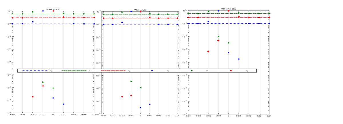
Figure 1: The distribution of ideal weights $d_{k}$ and non-linear weights $\omega_{k}$, $k=0,1,2$.

4.2 Linear advection test

Consider the linear advection equation (3.9) with the initial condition

$$u_{0}(x)=\begin{cases}\frac{1}{6}[G(x,z-\delta)+G(x,z)+4G(x,z+\delta)],&-0.8<x<0.2,\\ 1,&0.2\leq x\leq 0.8,\end{cases}$$ (4.2)

in a computational domain $[-1,1]$ where $G(x,z)=\exp(-\beta(x-z)^{2}),$ $z=-0.7$ and $\beta=\frac{\log(2)}{36\delta^{2}}$. This initial condition consists of Gaussian and square wave shapes. The numerical solution is displayed in Fig.2 for time $t=8$. From this, it is observed that WENO-UD5 schemes have the higher-resolution, better behavior in comparison to the WENO-LOC and WENO-JS5 schemes.

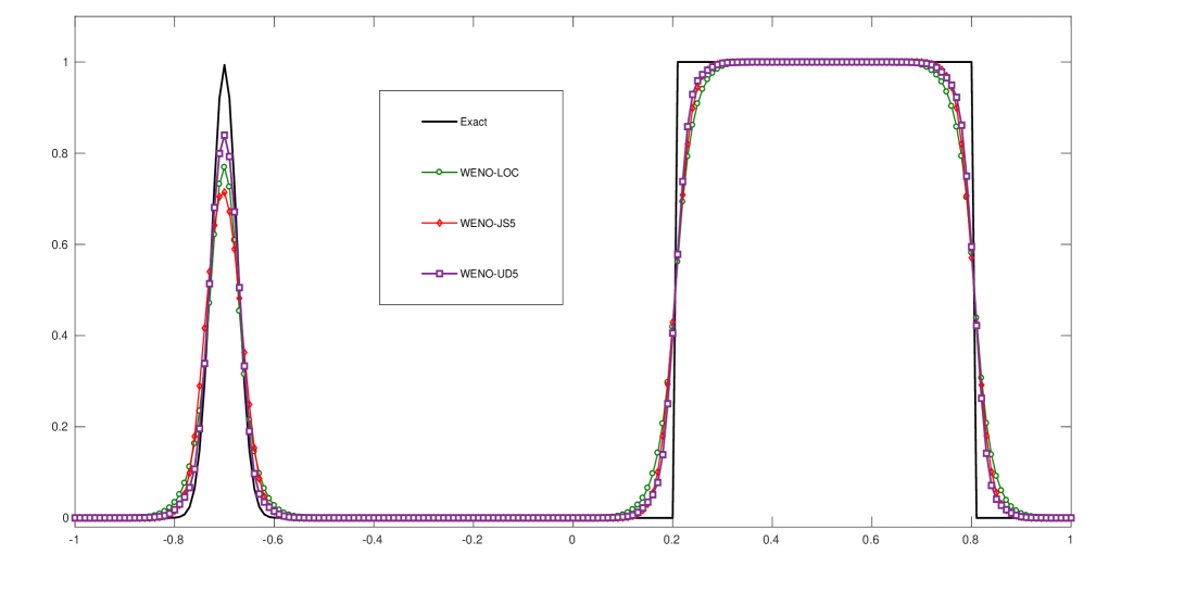
Figure 2: Numerical solution of (3.9) with initial condition (4.2)

4.3 One-dimensional Euler equations

The numerical simulations are performed on the one-dimensional Euler equations which are given by

$$\begin{pmatrix}\rho\\ \rho u\\ E\end{pmatrix}_{t}+\begin{pmatrix}\rho u\\ \rho u^{2}+p\\ u(E+p)\end{pmatrix}_{x}=0,$$ (4.3)

where $\rho,u,E,p$ are the density, velocity, total energy and pressure respectively. The system (4.3) represents the conservation of mass, momentum and energy. The total energy for an ideal polytropic gas is defined as

$$E=\frac{p}{\gamma-1}+\frac{1}{2}\rho u^{2},$$

and the eigenvalues of the Jacobian matrix $A(U)=\partial F/\partial U$ are

$$\lambda_{1}(u)=u-c,\quad\lambda_{2}(u)=u,\quad\lambda_{3}(u)=u+c,$$

where $U=\begin{pmatrix}\rho\\ \rho u\\ E\end{pmatrix}$, $F=\begin{pmatrix}\rho u\\ \rho u^{2}+p\\ u(E+p)\end{pmatrix}$ and $\gamma$ is the ratio of specific heats and its value is taken as $1.4$.

Remark: For the systems of conservation laws, such as one dimensional Euler equations, the reconstruction procedures are implemented in the local characteristic directions for the purpose of avoiding spurious oscillations. For the two dimensional problems, all of these reconstruction procedures are carried out in a dimension by dimension fashion.

4.3.1 Sod’s shock tube problem

We consider the one dimensional Euler system (4.3) with Riemann data [30]

$$(\rho,u,p)=\begin{cases}(1,0,1),&-5\leq x<0,\\ (0.125,0,0.1),&0\leq x\leq 5,\end{cases}$$

in the computational domain $-5\leq x\leq 5.$ The problem is initialized on the computational domain of $200$ points and is run up to time $t=1.3,$ by this time a right-going shock wave, a right traveling contact-wave and a left-sonic rarefaction wave establishes. The transmissive boundary conditions are taken for numerical evaluation. The numerical results of density profiles are displayed in the Fig.3. It is observed that the discontinuity is sharpened by WENO-UD$5$ schemes over WENO-LOC and WENO-JS5 schemes due to the efficient confinement of WENO dissipation right around the discontinuity.

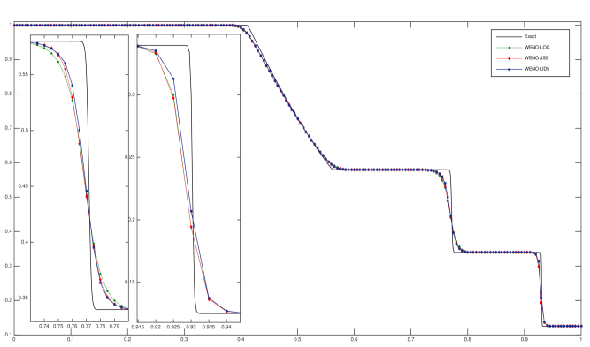
Figure 3: Sod problem: Density distribution for fifth-order WENO schemes

4.3.2 Lax’s shock tube problem

The initial condition

$$(\rho,u,p)=\begin{cases}(0.445,0.698,3.528),&-5\leq x<0,\\ (0.5,0,0.571),&0\leq x\leq 5,\end{cases}$$

is considered [31] to the one dimensional Euler system of equations (4.3). This shock test case is considered in the computational domain $-5\leq x\leq 5,$ and is run up to $t=1.3$ with the zero gradient boundary conditions. The numerical results of density profiles along with the reference solutions are displayed in the Fig.4. The observation from the figure reveals that the numerical solutions WENO-UD$5$ schemes have better resolution in comparison to WENO-LOC and WENO-JS5 schemes.

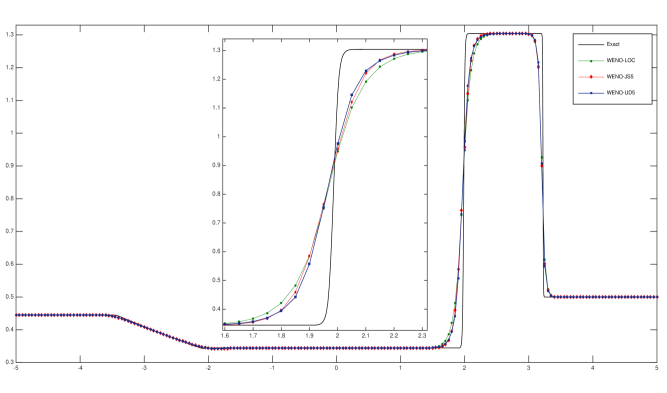
Figure 4: Lax problem: Density distribution for fifth-order WENO schemes

4.3.3 Mach 3 Shock entropy wave interaction test

For the system (4.3), consider the Riemann data

$$(\rho,u,p)=\begin{cases}(3.857143,2.629369,\frac{31}{3}),&-5\leq x<-4,\\ (1+0.2\sin(kx),0,1),&-4\leq x\leq 5,\end{cases}$$

on the spatial domain $x\in[-5,5]$ with $k=5.$ The solution of this problem [2] consists of a number of shocklets and fine scales structure, which are located behind a right going main shock. Fig.5 depicts the numerical results of WENO-LOC, WENO-JS5 and WENO-UD$5$ schemes for $N=200$ cells at time $t=1.8$ against the reference solution, computed by WENO-JS5 scheme with $N=2000$ points. We observed that WENO-UD$5$ capture more features of the solution than the WENO-LOC and WENO-JS5 particularly, at the high-frequency waves behind the shock at deeper valleys and higher pikes in the numerical solution.

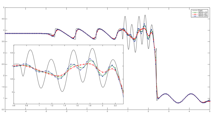
Figure 5: Solution of the Mach 3 shock density wave interaction with $k=5$ with $N=200$ points.

4.4 Two dimensional Euler system of equations

4.4.1 2D Riemann gas dynamics problem

The two-dimensional Riemann problem of gas dynamics [32] is defined by initial constant states which is divided by the lines $x=0.8$ and $y=0.8$ on the square as

$$(\rho,u,v,p) =\begin{cases}\begin{array}[]{lr}(1.5,0,0,1.5)&\text{if}\;0.8\leq x\leq 1,0.8\leq y\leq 1,\\ (0.5323,1.206,0,0.3)&\text{if}\;0\leq x<0.8,0.8\leq y\leq 1,\\ (0.138,1.206,1.206,0.029)&\text{if}\;0\leq x<0.8,0\leq y<0.8,\\ (0.5323,0,1.206,0.3)&\text{if}\;0.8<x\leq 1,0\leq y\leq 0.8,\end{array}\end{cases}$$

and the time evolution is governed by two-dimensional Euler equations,

$$\begin{pmatrix}\rho\\ \rho u\\ \rho v\\ p\end{pmatrix}_{t}+\begin{pmatrix}\rho u\\ P+\rho u^{2}\\ \rho uv\\ u(E+P)\end{pmatrix}_{x}+\begin{pmatrix}\rho v\\ \rho uv\\ P+\rho v^{2}\\ v(E+P)\end{pmatrix}_{y}=0.$$ (4.4)

The total energy $E$ and the pressure $p$ is defined by

$$p=(\gamma-1)(E-\frac{1}{2}\rho(u^{2}+v^{2})),$$

where $u$ and $v$ are $x$ and $y$-velocity components respectively. The numerical solution is computed on the computational domain $[0,1]\times[0,1]$ with Dirichlet boundary conditions on $400\times 400$ grid points. According to the initial conditions, four shocks come into being and produce a narrow jet. The numerical solution is calculated upto time $t=0.8$. The grid refinement results of WENO-LOC, WENO-JS5 and WENO-UD5 schemes are given in Fig.6 that contains the numerical solutions of WENO-LOC, WENO-JS5 and WENO-UD5 schemes. An examination of these results reveals that the WENO-UD$5$ scheme captures a better resolution of the fine structures in comparison to the schemes WENO-LOC and WENO-JS5 respectively.

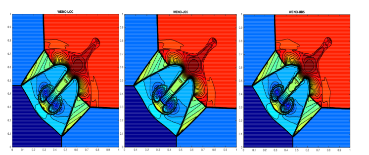
Figure 6: Density profile of 2D Riemann problem of gas dynamics

4.4.2 Double Mach reflection of a strong shock

For the Euler’s system (4.4), the two-dimensional double Mach reflection problem presented by Woodward and Colella in [33] is considered in this example on the domain of $[0,4]\times[0,1].$ The reflecting boundary conditions for $\frac{1}{6}\leq x\leq 4,y=0$ are taken. Initially, a right-moving Mach $10$ shock is positioned at $x=\frac{1}{6},y=0,$ and makes an angle of $60^{o}$ with the $x-$axis. For the bottom boundary $0\leq x<\frac{1}{6},y=0$, the exact post shock condition is imposed. The top boundary of our computational domain uses the exact motion of the Mach $10$ shock. Inflow and outflow boundary conditions are taken for the left and right boundaries. The unshocked fluid has a density $1.4$, pressure $1.$ and the ratio of specific heats $\gamma=1.4$. The numerical solution is computed up to time $t=0.2$ on a mesh $500\times 500.$ The results in the region $[0,4]\times[0,1]$ are displayed for WENO-LOC, WENO-JS5 and WENO-UD$5$ schemes are shown in Fig.9, 9 and 9 respectively. It can be clearly seen in Fig.10 that WENO-UD$5$ resolves the instabilities better around the Mach stem of the problem.

5 Conclusions

In this paper, we have constructed a new type of nonlinear weights for the fifth-order weighted essentially non-oscillatory scheme. These nonlinear weights have been developed by construction of a new global smoothness indicator using the linear combination of second-order derivative information of local stencils which resulted a sixth-order value on five point stencil. These nonlinear weights satisfies convexity, ENO property and achieves the optimal order of accuracy. The resulted numerical scheme achieved the desired fifth-order accuracy in the smooth regions and in presence of critical points. Further, we have analyzed the consistency analysis on the weight parameters and verified the ENO property theoretically as well as numerically. Numerical results resembled in scalar, system of one- and two-dimensional Euler equations for typical shock tube problems and double-Mach reflection of strong shock test cases.

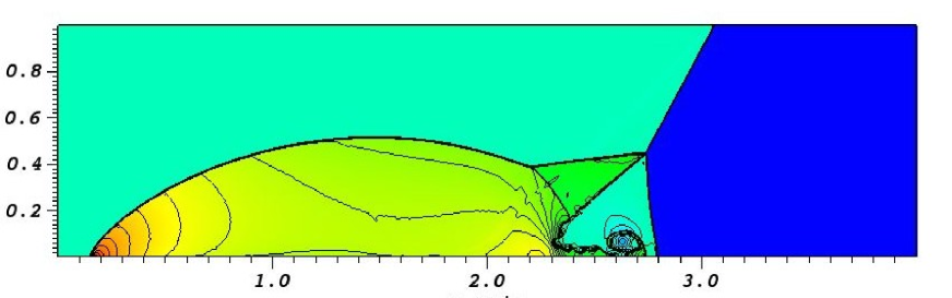
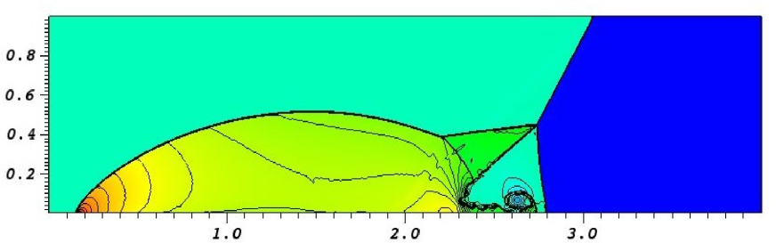
Figure 7: Density profile of double Mach reflection of a strong shock:WENO-LOC scheme

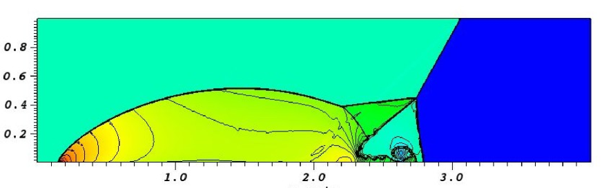
Figure 8: Density profile of double Mach reflection of a strong shock:WENO-JS5 scheme

Figure 9: Density profile of double Mach reflection of a strong shock:WENO-UD5 scheme

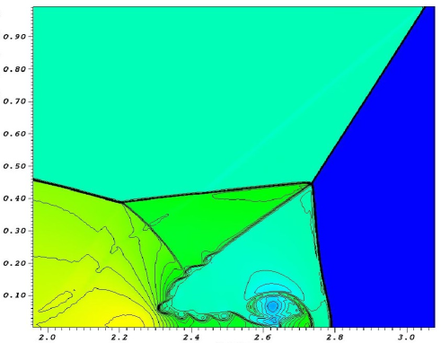
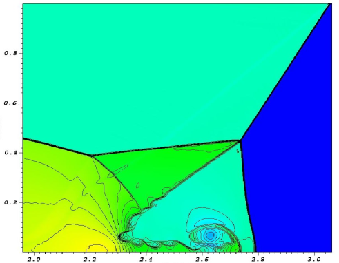
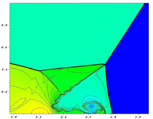
Figure 10: Density profile of double Mach reflection of a strong shock around Mach stem:WENO-LOC, JS5 and UD5 scheme

References

- [1] Harten, A., Engquist, B., Osher, S., Chakravarthy, S.R.: Uniformly high order accurate non-oscillatory schemes, III. J. Comput. Phys. 13, 13-47(1997).
- [2] Harten, A., Osher, S.: Uniformly high-order accurate non oscillatory schemes, I. SIAM J. Numer. Anal. 24, 279-309(1987).
- [3] Shu, C.W., Osher, S.: Efficient implementation of essentially non-oscillatory shock-capturing schemes. J. Comput. Phys. 77, 439-471(1998).
- [4] Shu, C.W., Osher, S.: Efficient implementation of essentially non-oscillatory shock-capturing schemes II. J. Comput. Phys. 83, 32-78( 1989).
- [5] Liu, X.D., Osher, S., Chan, T.: Weighted Essentially non-oscillatory schemes. J. Comput. Phys. 115, 200-212(1994).
- [6] Jiang, G.S., Shu, C.W.: Efficient implementation of Weighted ENO schemes. J. Comput. Phys. 126, 202-228(1996).
- [7] Balsara, D.S., Shu, C.W.: Monotonicity preserving weighted essentially non-oscillatory schemes with increasingly high order of accuracy. J. Comput. Phys. 160, 405-452(2000).
- [8] Gerolymos, G.A., Senechal, D., Vallet, I.: Very high order WENO schemes. J. Comput. Phys. 228, 8481-8524(2009).
- [9] Balsara, D.S., Rumpf, T., Dumbser, M., Munz, C.D.: Efficient, high-accuracy ADER-WENO schemes for hydrodynamics and divergence-free magnetohydro-dynamics. J. Comput. Phys. 228, 2480-2516(2009).
- [10] Balsara, D.S., Garain, S., Shu, C.W.: An efficient class of WENO schemes with adaptive order. J. Comput. Phys. 326, 780-804(2016).
- [11] Henrick, A.K., Aslam, T.D., Powers, J.M.: Mapped weighted essentially non-oscillatory schemes: Achieving optimal order near critical points. J. Comput. Phys. 207, 542-567(2005).
- [12] Borges, R., Carmona, M., Costa, B., Don, W.S.: An improved weighted essentially non-oscillatory scheme for hyperbolic conservation laws. J. Comput. Phys. 227, 3191-3211(2008).
- [13] Castro, M., Costa, B., Don, W.S.: High order weighted essentially nonoscillatory WENO-Z schemes for hyperbolic conservation laws. J. Comput. Phys. 230, 766-792(2011).
- [14] Ha, Y., Kim, C.H., Lee, Y.J., Yoon, J.: An improved weighted essentially non-oscillatory scheme with a new smoothness indicator. J. Comput. Phys. 232, 68-86(2013).
- [15] Kim, C.H., Ha, Y., Yoon, J.: Modified Non-linear Weights for Fifth-Order Weighted Essentially Non-oscillatory Schemes. J. Sci. Comput. 67, 299-323(2016).
- [16] Rathan, S., Raju, G.N.: A modified fifth-order WENO scheme for hyperbolic conservation laws, Comput. Math. Appl. 75, 1531-1549(2018).
- [17] Rathan, S., Raju, G.N.: An improved nonlinear weights for seventh-order weighted essentially non-oscillatory scheme. Comput. Fluids. 156, 496-514(2017).
- [18] Rathan, S., Raju, G.N.: Improved weighted ENO scheme based on parameters involved in nonlinear weights. Appl. Math. Comput. 331, 120-129(2018).
- [19] Serna, S., Marquina, A.: Power-ENO methods: a fifth-order accurate weighted power ENO method, J. Comput. Phys. 194, 632-658(2004).
- [20] Fan, P., Shen, Y., Tian, B., Yang, C.: A new smoothness indicator for improving the weighted essentially non-oscillatory scheme, J. Comput. Phys. 269, 329-354(2014).
- [21] Fan, P.: High order weighted essentially non oscillatory WENO-schemes for hyperbolic conservation laws, J. Comput. Phys. 269, 355-285(2014).
- [22] Feng, H., Hu, F.X., Wang, R.: A new mapped weighted essentially non-oscillatory scheme, J. Sci. Comput. 51, 449-473(2012).
- [23] Wang, R., Feng, H., Huang, C.: A new mapped weighted essentially non-oscillatory method with rational mapping function, J. Sci. Comput. 67, 540-580(2016).
- [24] Yamaleev, NK, Carpenter M.H.: A systematic methodology for constructing high-order energy stable WENO schemes, J. Comput. Phys. 228, 4248-4272(2009).
- [25] Biswas, B., Dubey, R. K.: Accuracy Preserving ENO and WENO Schemes using Novel Smoothness Measurement. arXiv preprint arXiv:1809.07956(2018).
- [26] Fu, L, Hu, X.Y., and Nikolaus A.: A family of high-order targeted ENO schemes for compressible-fluid simulations. J. Comput. Phys. 305, 333-359(2016):
- [27] Gottlieb, S.: On high order strong stability preserving Runge–Kutta and multi- step time discretizations. J. Sci. Comput. 25,105-128(2005).
- [28] Leveque, R.J.: Numerical Methods for Conservation Laws, Birkhauser Verlag, 1992(Lectures in Mathematics ETH Zurich).
- [29] Don, W.S., Borges, R.: Accuracy of the weighted essentially nonoscillatory WENO-Z scheme for hyperbolic conservation laws, J. Comput. Phys. 230, 766-792(2013).
- [30] Sod, G.A.: A survey of several finite difference methods for systems of nonlinear hyperbolic conservation laws. J. Comput. Phys. 107, 1-31( 1978).
- [31] Lax, P.D.: Weak solutions of nonlinear hyperbolic equations and their numerical computation. Commu. Pure. Appl. Math. 7, 159-193(1954).
- [32] Schulz-Rinne, C.W., Collins, J.P., Glaz, H.M.: Numerical solution of the Riemann problem for two-dimensional gas dynamics. SIAM J. Sci. Comput. 14, 1394-1414(1993).
- [33] Woodward, P., Colella, P.: The numerical simulation of two-dimensional fluid flow with strong shocks. J. Comput. Phys. 54, 115-173(1984).
- [34] Kumar, R., Chandrashekar, P.: Simple smoothness indicator and multi-level adaptive order WENO scheme for hyperbolic conservation laws. Journal of Computational Physics, 375, 1059-1090(2018).