Numerical approach to the semiclassical method of radiation emission for arbitrary electron spin and photon polarization

Abstract

We show how the semiclassical formulas for radiation emission of Baier, Katkov and Strakhovenko for arbitrary initial and final spins of the electron and arbitrary polarization of the emitted photon can be rewritten in a form which numerically converges quickly. We directly compare the method in the case of a background plane wave with the result obtained by using the Volkov state solution of the Dirac equation, and confirm that we obtain the same result. We then investigate the interaction of a circularly polarized short laser pulse scattering with GeV electrons and see that the finite duration of the pulse leads to a lower transfer of circular polarization than that predicted by the known formulas in the monochromatic case. We also see how the transfer of circular polarization from the laser beam to the gamma ray beam is gradually deteriorated as the laser intensity increases, entering the nonlinear regime. However, this is shown to be recovered if the scattered photon beam is collimated to only allow for passage of photons emitted with angles smaller than $1/\gamma$ with respect to the initial electron direction, where $\gamma$ is the approximately constant Lorentz factor of the electron. The obtained formulas also allow us to answer questions regarding radiative polarization of the emitting particles. In this respect we briefly discuss an application of the present approach to the case of a bent crystal and high-energy positrons.

I Introduction

The semiclassical formalism of Baier, Katkov and Strakhovenko allows for the approximate determination of the spectrum of emitted photons from an ultrarelativistic electron in a virtually arbitrary external electromagnetic field Baier et al. (1998). For numerical applications the formulation with a single time integration as found in Belkacem et al. (1985); Wistisen (2014) for the spin and polarization averaged result, is most useful. In this paper we show how the basic result of the semiclassical method with explicit electron spin and photon polarization can also be treated numerically in a similar fashion. We use the obtained formulas in the case of a background plane wave, as the Dirac equation then can be solved analytically Volkov (1935), to do a direct comparison with the spectrum obtained using the exact solution of the Dirac equation (Volkov states) Volkov (1935); Boca and Florescu (2010); Di Piazza (2018). This is the usual approach for such processes Ritus (1985); Seipt and Kämpfer (2012); Mackenroth and Di Piazza (2011); Dinu and Torgrimsson (2019); Boca and Florescu (2009); Seipt and Kämpfer (2011); Di Piazza et al. (2012); Harvey et al. (2009); Hu et al. (2010); Meuren et al. (2016); Ilderton (2011); Voroshilo et al. (2015); Krajewska and Kamiński (2012a, b); Seipt et al. (2018); Angioi et al. (2016). We consider the case of a short circularly polarized laser pulse, and find agreement, as expected. The advantage of the presented approach is the possibility of calculating the radiation emission under general circumstances, i.e. also for very complicated field configurations as one only needs the classical trajectory in the external field, which can easily be found numerically for a given field. The presented formulas allow to find the polarization properties of the radiation depending on the spin of the initial and final electron, which also allows to determine if the electrons become polarized. The latter would occur if the spin-flip radiation has a different yield for each of the possible initial spin states, see e.g. Jackson (1976), i.e. a generalization of the Sokolov-Ternov effect Sokolov and Ternov (1966) to fields other than that of a permanent magnetic field Del Sorbo et al. (2017); Li et al. (2019). We briefly demonstrate this in the case of positrons channeling in a bent germanium crystal where one has two kinds of motion superimposed, the oscillatory channeling motion between the bent planes, which in the unbent case would not lead to polarization, along with the motion along the bending arc which leads to transverse polarization of the positrons. When the crystal is strongly bent, i.e. close to the so-called Tsyganov radius Elishev et al. (1979); Tsyganov (1976), the polarization as in a magnetic field is obtained, while smaller bending radii lead to smaller degrees of polarization, which the presented method allows to predict.

Below, $e$ indicates the positron charge, and units are used, such that the fine-structure constant $\alpha$ is given by $e^{2}$, whereas the relativistic metric $+---$ is employed. We will use Feynman notation to write $\not{a}=a_{\mu}\gamma^{\mu}$, where $a^{\mu}$ is a generic 4-vector.

II Semiclassical approach

Below, we study the emission by an electron of a single photon in a given background electromagnetic field. The basic result of the semiclassical method of Baier et al. in its most general form for the single-photon radiation probability is expressed as Baier et al. (1998)

$$dP=\frac{\alpha\omega}{(2\pi)^{2}}\left|\int_{-\infty}^{\infty}R(t)e^{ik^{\prime}x}dt\right|^{2}d\Omega d\omega,$$ (1)

where $x^{\mu}=\{t,\boldsymbol{x}(t)\}$ is the electron 4-position as obtained by the Lorentz force equation in the external field, $k^{\prime\mu}=\omega^{\prime}\{1,\boldsymbol{n}\}$, $\omega^{\prime}=\frac{\varepsilon}{\varepsilon^{\prime}}\omega$, $\omega$ is the energy of the emitted photon, $\varepsilon^{\prime}=\varepsilon-\omega$, $\varepsilon$ the electron energy, $\boldsymbol{n}$ the direction of emission, and

$$R(t)=\phi_{f}^{\dagger}\left[A(t)+i\boldsymbol{\sigma}\cdot\boldsymbol{B}(t)\right]\phi_{i}.$$ (2)

Here, $\phi_{i}$ and $\phi_{f}$ are the spinors of the initial and final electron state (characterized by the electron 4-momentum and the electron spin in its asymptotic rest frame), $\boldsymbol{\sigma}$ denotes the vector of the Pauli spin matrices, and

$$A(t) =C\boldsymbol{\epsilon}^{*}\cdot\boldsymbol{v}(t),$$ (3)

$$\boldsymbol{B}(t) =\boldsymbol{\epsilon}^{*}\times\left[D_{1}\boldsymbol{v}(t)+D_{2}\boldsymbol{n}\right],$$ (4)

with $\boldsymbol{\epsilon}$ being the polarization vector of the emitted photon, $\boldsymbol{v}(t)=d\boldsymbol{x}(t)/dt$ being the electron velocity, and the constants being given by

$$C=\frac{\varepsilon}{2\sqrt{\varepsilon\varepsilon^{\prime}}}\left[\sqrt{\frac{\varepsilon^{\prime}+m}{\varepsilon+m}}+\sqrt{\frac{\varepsilon+m}{\varepsilon^{\prime}+m}}\right],$$ (5)

$$D_{1}=\frac{\varepsilon}{2\sqrt{\varepsilon\varepsilon^{\prime}}}\left[\sqrt{\frac{\varepsilon^{\prime}+m}{\varepsilon+m}}-\sqrt{\frac{\varepsilon+m}{\varepsilon^{\prime}+m}}\right],$$ (6)

$$D_{2}=\frac{\omega}{2\sqrt{\varepsilon\varepsilon^{\prime}}}\sqrt{\frac{\varepsilon+m}{\varepsilon^{\prime}+m}}.$$ (7)

To evaluate the quantity in Eq. (1) we need to carry out the two time integrals $\int\boldsymbol{v}(t)e^{ik^{\prime}x}dt$ and $\int e^{ik^{\prime}x}dt$. However, a direct computation of these integrals converges slowly, and integrations beyond times when the acceleration is different from zero must be included, as explained classically in Jackson (1991). From the relations shown in Wistisen (2014), and which are already used there in the case without polarization and spin averaging, it is quite easy to relate these quantities to the quantities whose integrands are proportional to the acceleration. By doing this, we have that

$$\int_{-\infty}^{\infty}\boldsymbol{v}(t)e^{ik^{\prime}x}dt=\frac{i}{\omega^{\prime}}\left(\boldsymbol{n}J-\boldsymbol{I}\right),$$ (8)

$$\int_{-\infty}^{\infty}e^{ik^{\prime}x}dt=\frac{i}{\omega^{\prime}}J,$$ (9)

where

$$\boldsymbol{I}=\int_{-\infty}^{\infty}\frac{\boldsymbol{n}\times\left[\left(\boldsymbol{n}-\boldsymbol{v}\right)\times\dot{\boldsymbol{v}}\right]}{\left(1-\boldsymbol{n}\cdot\boldsymbol{v}\right)^{2}}e^{ik^{\prime}x}dt,$$ (10)

$$J=\int_{-\infty}^{\infty}\frac{\boldsymbol{n}\cdot\dot{\boldsymbol{v}}}{\left(1-\boldsymbol{n}\cdot\boldsymbol{v}\right)^{2}}e^{ik^{\prime}x}dt.$$ (11)

In Wistisen (2014) it is shown in detail how to calculate the electron trajectory and the quantities $\boldsymbol{I}$ and $J$ numerically. In particular it is appropriate to analytically carry out the cancellations between large terms, as in e.g. $1-\boldsymbol{n}\cdot\boldsymbol{v}$ because $\boldsymbol{n}\cdot\boldsymbol{v}$ is close to $1$ for ultrarelativistic particles. Finally, we may write

$$\int_{-\infty}^{\infty}R(t)e^{ik^{\prime}x}dt$$

$$=-\frac{i}{\omega^{\prime}}\phi_{f}^{\dagger}\left[C\boldsymbol{\epsilon}^{*}\cdot\boldsymbol{I}\right.$$

$$\left.+i\boldsymbol{\sigma}\cdot\left(\boldsymbol{\epsilon}^{*}\times\left[\boldsymbol{I}D_{1}-(D_{1}+D_{2})\boldsymbol{n}J\right]\right)\right]\phi_{i},$$ (12)

and therefore we obtain the emission probability as

$$\frac{dP}{d\Omega} =\frac{\alpha}{(2\pi)^{2}}\frac{\omega}{\omega^{\prime 2}}$$

$$\times\left|\phi_{f}^{\dagger}\left[C\boldsymbol{\epsilon}^{*}\cdot\boldsymbol{I}\right.\right.$$

$$\left.+i\boldsymbol{\sigma}\cdot\left(\boldsymbol{\epsilon}^{*}\times\left[\boldsymbol{I}D_{1}-(D_{1}+D_{2})\boldsymbol{n}J\right]\right)\right]\phi_{i}\Big{|}^{2}$$ (13)

III Volkov-state approach

If the background field is a plane wave, i.e. if the 4-vector potential $A^{\mu}(\varphi)$ only depends on the phase $\varphi=k_{0}x$, where $k_{0}=(\omega_{0},\boldsymbol{k}_{0})$ is the 4-momentum associated with the photons of the plane wave, the corresponding Dirac equation

$$\left(i\not{\partial}+e\not{A}-m\right)\psi=0,$$ (14)

can be solved analytically Volkov (1935). Below we assume that the plane wave propagates along the negative $z$ direction and we choose 4-vector potential $A^{\mu}(\varphi)$ in the Lorenz gauge where $A^{0}(\varphi)=A^{3}(\varphi)=0$. The positive-energy solution reads

$$\psi(x)=\frac{1}{\sqrt{2\varepsilon}}\left(1-\frac{e\not{k}_{0}\not{A}}{2k_{0}p}\right)ue^{iS},$$ (15)

where $p$ is the asymptotic 4-momentum of the electron, (we have set the quantization volume equal to $1$), where

$$S=-px+\frac{e}{k_{0}p}\int^{\varphi}d\varphi^{\prime}\left[pA(\varphi^{\prime})+\frac{e}{2}A^{2}(\varphi^{\prime})\right]$$ (16)

is the classical action of the electron in the plane wave, and where $u$ is a short notation for the constant vacuum bispinor (which is characterized by the electron spin in the corresponding electron rest frame and by the electron 4-momentum $p$). The leading-order matrix element for single-photon emission is given by

$$S_{fi}=ie\sqrt{\frac{4\pi}{2\omega}}\int d^{4}x\bar{\psi}_{f}(x)\not{\epsilon}^{*}e^{ikx}\psi_{i}(x),$$ (17)

where $\psi_{i/f}(x)$ indicates the Volkov state corresponding to the initial/final electron state, and the differential probability of emission is then

$$dP=\left|S_{fi}\right|^{2}\frac{d^{3}p_{f}}{(2\pi)^{3}}\frac{d^{3}k}{(2\pi)^{3}}.$$ (18)

In the gauge we are working, the 4-potential can be written as

$$A^{\mu}(\varphi)=\sum_{j=1}^{2}a_{j}^{\mu}f_{j}(\varphi),$$ (19)

where $a_{j}^{\mu}$ are two 4-vectors such that $a_{j}k_{0}=0$ and $a_{1}a_{2}=0$ and where $f_{j}(\varphi)$ are two arbitrary (physically well-behaved) functions. By setting the arbitrary phase in the indefinite integrals in the phase of Volkov states to zero, we introduce the quantities

$$F_{j}(\varphi)=\int_{0}^{\varphi}f_{j}(\varphi^{\prime})d\varphi^{\prime},$$ (20)

$$G_{j}(\varphi)=\int_{0}^{\varphi}f_{j}^{2}(\varphi^{\prime})d\varphi^{\prime}.$$ (21)

Then, by inserting the expressions of Eqs. (15) and (19) into Eq. (17), we obtain that

$$S_{fi} =ie\sqrt{\frac{4\pi}{2\omega}}\frac{1}{\sqrt{4\varepsilon_{f}\varepsilon_{i}}}\int d^{4}x$$

$$\bar{u}_{f}\left(\not{\epsilon}^{*}+\sum_{j=1}^{2}\left[B_{j}f_{j}(\varphi)+C_{j}f_{j}(\varphi)^{2}\right]\right)u_{i}$$

$$\times e^{-i(p_{i}-p_{f}-k)x}e^{i\left(\sum_{j=1}^{2}\left[\alpha_{j}F_{j}(\varphi)+\beta_{j}G_{j}(\varphi)\right]\right)},$$ (22)

where we have defined

$$\alpha_{j}=e\left[\frac{p_{i}a_{j}}{k_{0}p_{i}}-\frac{p_{f}a_{j}}{k_{0}p_{f}}\right],$$ (23)

$$\beta_{j}=\frac{e^{2}a_{j}^{2}}{2}\left[\frac{1}{k_{0}p_{i}}-\frac{1}{k_{0}p_{f}}\right],$$ (24)

and

$$B_{j}=-\left[\frac{e\not{a}_{j}\not{k}_{0}}{2k_{0}p_{f}}\not{\epsilon}^{*}+\not{\epsilon}^{*}\frac{e\not{k}_{0}\not{a}_{j}}{2k_{0}p_{i}}\right],$$ (25)

$$C_{j} =\frac{e\not{a}_{j}\not{k}_{0}}{2k_{0}p_{f}}\not{\epsilon}^{*}\frac{e\not{k}_{0}\not{a}_{j}}{2k_{0}p_{i}}$$

$$=-\frac{e^{2}a_{j}^{2}}{2\left(k_{0}p_{f}\right)\left(k_{0}p_{i}\right)}\left(\epsilon^{*}k_{0}\right)\not{k}_{0},$$ (26)

with $j=1,2$ (we have set $\epsilon^{\mu}=(0,\boldsymbol{\epsilon})$). Now, we can write the functions in Eq. (22) as a Fourier transform

$$f_{j}^{n}(\varphi)e^{i\left(\sum_{j=1}^{2}\left[\alpha_{j}F_{j}(\varphi)+\beta_{j}G_{j}(\varphi)\right]\right)}$$

$$=\int_{-\infty}^{\infty}A_{n,j}(s,\alpha,\beta)e^{-is\varphi}ds,$$ (27)

where

$$A_{n,j}(s,\alpha,\beta)$$

$$=\frac{1}{2\pi}\int_{-\infty}^{\infty}d\varphi f_{j}^{n}(\varphi)e^{i\left(s\varphi+\sum_{j=1}^{2}\left[\alpha_{j}F_{j}(\varphi)+\beta_{j}G_{j}(\varphi)\right]\right)},$$ (28)

defined for $n=0,1,2$. When $n=0$, the $j$ subscript is superfluous and we will therefore denote this function as $A_{0}(s,\alpha,\beta)$. This function is however problematic as it diverges but it can be regularized by using the identity (see also Boca and Florescu (2009); Seipt and Kämpfer (2011); Mackenroth and Di Piazza (2011))

$$0 =\int_{-\infty}^{\infty}e^{ih(\varphi)}h^{\prime}(\varphi)d\varphi,$$ (29)

where

$$h(\varphi)=s\varphi+\sum_{j=1}^{2}\left[\alpha_{j}F_{j}(\varphi)+\beta_{j}G_{j}(\varphi)\right].$$ (30)

In this way, we obtain

$$A_{0}(s,\alpha,\beta) =$$

$$=\frac{1}{2\pi}\int_{-\infty}^{\infty}e^{i\left(s\varphi+\sum_{j=1}^{2}\left[\alpha_{j}F_{j}(\varphi)+\beta_{j}G_{j}(\varphi)\right]\right)}d\varphi$$

$$=-\frac{1}{s}\sum_{j=1}^{2}\left[\alpha_{j}A_{1,j}+\beta_{j}A_{2,j}\right].$$ (31)

By replacing these expressions in Eq. (22), and carrying out the integration over $d^{4}x$, we can write the amplitude in the form

$$S_{fi} =ie\sqrt{\frac{4\pi}{2\omega}}\frac{1}{\sqrt{4\varepsilon_{f}\varepsilon_{i}}}\int ds(2\pi)^{4}\delta^{4}(p_{i}-p_{f}-k+sk_{0})$$

$$\times\bar{u}_{f}\left(\not{\epsilon}^{*}A_{0}+\sum_{j=1}^{2}\left[B_{j}A_{1,j}+C_{j}A_{2,j}\right]\right)u_{i}.$$ (32)

Now we can use the energy delta function to fix $s$ such that

$$s_{0}=\frac{\varepsilon_{f}+\omega-\varepsilon_{i}}{\omega_{0}},$$ (33)

and the delta function can be transformed as $\delta(\varepsilon_{i}-\varepsilon_{f}-\omega+s\omega_{0})=\frac{1}{\omega_{0}}\delta(s-s_{0})$:

$$S_{fi}= ie\sqrt{\frac{4\pi}{2\omega}}\frac{1}{\sqrt{4\varepsilon_{f}\varepsilon_{i}}}(2\pi)^{4}\frac{1}{\omega_{0}}\delta^{3}(\boldsymbol{p}_{i}-\boldsymbol{p}_{f}-\boldsymbol{k}+s_{0}\boldsymbol{k}_{0})$$

$$\times\bar{u}_{f}\left(\not{\epsilon}^{*}A_{0}+\sum_{j=1}^{2}\left[B_{j}A_{1,j}+C_{j}A_{2,j}\right]\right)u_{i}.$$ (34)

At this point we would then take the norm-square to obtain the transition probability, however we are then faced with the problem of how to take the square of the delta-function which has the complication that $s_{0}$ is a function of the momenta. The correct way to do this, is to consider instead the more realistic case of an initial wave packet $\Psi_{i}(x)=\int\psi_{\boldsymbol{p}_{i}}(x)c(\boldsymbol{p}_{i})d^{3}\boldsymbol{p}_{i}$ where $\psi_{\boldsymbol{p}_{i}}(x)$ is the Volkov solution with momentum $\boldsymbol{p}_{i}$ and unindicated fixed spin quantum number. To preserve normalization we must have that $\int\left|c(\boldsymbol{p}_{i})\right|^{2}d^{3}\boldsymbol{p}_{i}=1/(2\pi)^{3}$. Then the momentum delta-function can be transformed as

$$\delta^{3}(\boldsymbol{p}_{i}-\boldsymbol{p}_{f}-\boldsymbol{k}+s_{0}(\boldsymbol{p}_{i})\boldsymbol{k}_{0})=\frac{1}{|\mathcal{J}_{i}|}\delta^{3}(\boldsymbol{p}_{i}-\boldsymbol{p}_{i,\text{sol}}),$$ (35)

where $\mathcal{J}_{i}=\partial\boldsymbol{g}/\partial\boldsymbol{p}_{i}=I-\frac{\boldsymbol{k}_{0}\boldsymbol{p}_{i}^{T}}{\omega_{0}\varepsilon_{i}}$, is the Jacobian matrix with $\boldsymbol{g}\left(\boldsymbol{p}_{i}\right)=\boldsymbol{p}_{i}-\boldsymbol{p}_{f}-\boldsymbol{k}+s_{0}(\boldsymbol{p}_{i})\boldsymbol{k}_{0}$, $\boldsymbol{g}(\boldsymbol{p}_{i,\text{sol}})=\boldsymbol{0}$ ($\boldsymbol{k}_{0}\boldsymbol{p}_{i}^{T}$ indicates the dyadic product between the vectors $\boldsymbol{k}_{0}$ and $\boldsymbol{p}_{i}$), and so using Sylvester’s determinant theorem we obtain

$$|\mathcal{J}_{i}|=\text{det}\left(I-\frac{\boldsymbol{k}_{0}\boldsymbol{p}_{i}^{T}}{\omega_{0}\varepsilon_{i}}\right)=1-\frac{\boldsymbol{k}_{0}\cdot\boldsymbol{p}_{i}}{\omega_{0}\varepsilon_{i}}=\frac{k_{0}p_{i}}{\omega_{0}\varepsilon_{i}}.$$ (36)

Therefore we finally write the transition amplitude in the form

$$S_{fi}= ie\sqrt{\frac{4\pi}{2\omega}}\frac{1}{\sqrt{4\varepsilon_{f}\varepsilon_{i}}}(2\pi)^{4}\frac{\varepsilon_{i}}{k_{0}p_{i}}$$

$$\times c(\boldsymbol{p}_{f}+\boldsymbol{k}-s_{0}(\boldsymbol{p}_{i,\text{sol}},\boldsymbol{p}_{f})\boldsymbol{k}_{0})$$ (37)

$$\times\bar{u}_{f}\left(\not{\epsilon}^{*}A_{0}+\sum_{j=1}^{2}\left[B_{j}A_{1,j}+C_{j}A_{2,j}\right]\right)u_{i}.$$ (38)

Now, in order to find the probability using Eq. (18) we take the norm-square of the above amplitude and, having in mind the case of a narrow wave packet Angioi et al. (2016), replace $\left|c(\boldsymbol{p}_{i})\right|^{2}=\delta^{3}(\boldsymbol{p}_{i}-\boldsymbol{p}_{i,0})/(2\pi)^{3}$. Analogously as above, we now have a delta-function which we can evaluate by integration over $d^{3}\boldsymbol{p}_{f}$ and the transformation of the delta-function yields a factor of $\frac{\omega_{0}\varepsilon_{f}}{k_{0}p_{f}}$. Finally, we then obtain the differential emission probability

$$dP =\left|\bar{u}_{f}\left(\not{\epsilon}^{*}A_{0}+\sum_{j=1}^{2}\left[B_{j}A_{1,j}+C_{j}A_{2,j}\right]\right)u_{i}\right|^{2}$$

$$\times\frac{e^{2}}{4}\frac{1}{\left(k_{0}p_{i}\right)\left(k_{0}p_{f}\right)}\omega d\omega d\Omega,$$ (39)

which can now be evaluated numerically. The bispinors in this expression are chosen as Berestetskii et al. (1971)

$$u=\sqrt{\varepsilon+m}\left(\begin{array}[]{c}\phi\\ \frac{\boldsymbol{\sigma}\cdot\boldsymbol{p}}{\varepsilon+m}\phi\end{array}\right),$$ (40)

where $\phi$ are spinors to be chosen as an orthonormal basis of eigenstates of $\boldsymbol{\sigma}\cdot\boldsymbol{s}$, with $\boldsymbol{s}$ being the direction of the otherwise arbitrary spin quantization axis in the rest frame of the electron.

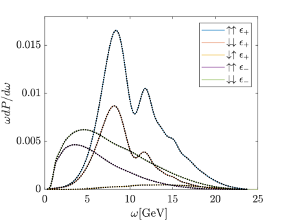
Figure 1: The intensity spectrum $\omega dP/d\omega$ according to the semiclassical approach is shown as solid lines corresponding to the different possibilities of initial and final spins and photon polarizations. The black dotted curves on top of the solid curves indicate the same quantities but calculated using the Volkov-states approach. We have not plotted the curve corresponding to $\uparrow\downarrow\boldsymbol{\epsilon}_{+}$ and $\downarrow\uparrow\boldsymbol{\epsilon}_{-}$ as the corresponding yields are much smaller than the others and the curves would not be visible. Also, we have not plotted $\uparrow\downarrow\boldsymbol{\epsilon}_{-}$ as it coincides with $\downarrow\uparrow\boldsymbol{\epsilon}_{+}$. In all these cases, the two approaches also agree.

IV Discussion of results

The above derivations were carried out without introducing a particular plane-wave pulse. We will now consider a particular choice of the 4-vector potential and carry out the corresponding numerical calculation using the semiclassical method and the Volkov-states method. We set $a_{1}^{\mu}=\{0,a_{x},0,0\}$, $a_{2}^{\mu}=\{0,0,a_{y},0\}$, $k^{\mu}=\{\omega_{0},0,0,-\omega_{0}\}$, and

$$f_{1}(\varphi)=d(\varphi)\text{cos}(\varphi),$$ (41)

$$f_{2}(\varphi)=d(\varphi)\text{sin}(\varphi),$$ (42)

$$d(\varphi) =\begin{cases}\text{sin}^{4}\left(\frac{\varphi}{2N}\right),&0<\varphi<2\pi N,\\ 0&\text{otherwise},\end{cases}$$ (43)

that is, we choose a pulse with envelope $d(\varphi)$ and negative helicity (right-handed) circular polarization .

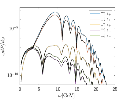
Figure 2: Integrated intensity of radiation as in Fig. (1) but with a collimation angle of $0.1/\gamma$, as explained in the text.

We define the polarizations of the outgoing light as

$$\boldsymbol{\epsilon}_{\pm}=\frac{1}{\sqrt{2}}\left(\boldsymbol{\epsilon}_{1}\pm i\boldsymbol{\epsilon}_{2}\right),$$ (44)

where

$$\boldsymbol{\epsilon}_{1}=\frac{\hat{\boldsymbol{y}}\times\boldsymbol{k}}{\left|\hat{\boldsymbol{y}}\times\boldsymbol{k}\right|},$$ (45)

with $\hat{\boldsymbol{y}}$ being the unit vector in the $y$ direction, and

$$\boldsymbol{\epsilon}_{2}=\frac{\boldsymbol{k}\times\boldsymbol{\epsilon}_{1}}{\left|\boldsymbol{k}\times\boldsymbol{\epsilon}_{1}\right|}.$$ (46)

According to this choice $\boldsymbol{\epsilon}_{1}$ and $\boldsymbol{\epsilon}_{2}$ are unit vectors orthogonal to each other and to $\boldsymbol{k}$ and such that, if $\boldsymbol{k}$ lies along the $z$ axis, they indicate the polarization along the $x$ and $y$ direction, respectively. The $\boldsymbol{\epsilon}_{\pm}$ basis corresponds to circular polarization with helicity of $\pm 1$. As the spin basis we have chosen quantization axis along the $z$ direction such that $\phi$ may be chosen as $\left(\begin{array}[]{cc}1&0\end{array}\right)^{T}$or $\left(\begin{array}[]{cc}0&1\end{array}\right)^{T}$, denoted by $\uparrow$ and $\downarrow$, respectively in the figures. We set $a_{x}=a_{y}=m\xi/e$, where $\xi$ is the classical nonlinearity parameter, which we have set $\xi=1$, $N=5$, and the electron energy $\varepsilon=30$ GeV for the Figs. (1), (2) and (3). Since the typical emission angles are small, we write $k_{x}=\omega\theta_{x}$ and $k_{y}=\omega\theta_{y}$ and then $d\Omega=d\theta_{x}d\theta_{y}$. In Fig. (1) we have restricted the angular integration such that $|\theta_{x}|<(\xi+3)/\gamma$, where $\gamma$ is the initial Lorentz factor of the electron, and the same for $\theta_{y}$ such that nearly all emitted radiation is included. In this figure we compare the semiclassical approach based on the formulas of Baier, Katkov and Strakhovenko and compare with the results obtained using the Volkov states. The results indicate nearly perfect agreement between the two approaches, which is expected since the motion in a plane wave is intrinsically semiclassical Ritus (1985). In Fig. (2) we do the same but restrict the emission angles over a smaller interval (collimation) i.e. $|\theta_{x}|<0.1/\gamma$ and the same for $\theta_{y}$. In this case the emitted radiation with negative helicity is highly suppressed and therefore we plotted the results on a logarithmic scale. This is expected due to angular momentum conservation along the $z$ axis. Since the electron flipping its spin is unlikely for ultrarelativistic electrons Berestetskii et al. (1971), the outgoing light must have opposite helicity as that of the laser field to conserve angular momentum. Finally, the agreement between the semiclassical method and the Volkov-state method in this case indicates an agreement of the two approaches also at the level of angularly resolved spectra.

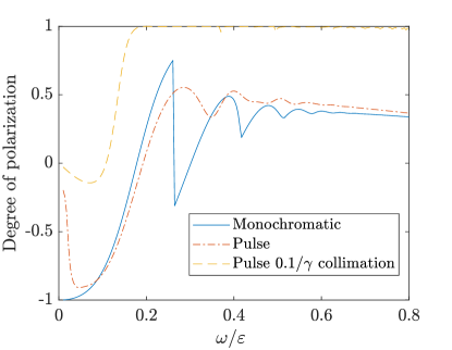
Figure 3: Degree of circular polarization of the Compton scattered radiation for nonlinear Compton scattering in a monochromatic wave without collimation, and in the short pulse described in the text with and without angular collimation.

In Fig. (3) we show how the collimation affects the degree of circular polarization, defined as

$$\mathcal{P}=\frac{\frac{dP^{+}}{d\omega}-\frac{dP^{-}}{d\omega}}{\frac{dP^{+}}{d\omega}+\frac{dP^{-}}{d\omega}}.$$ (47)

We compare with the result found in Ivanov et al. (2004), obtained in the case of the monochromatic wave, and see that in the short pulse one reaches a slightly smaller value. However, if one collimates the photon beam, one can achieve circular polarization to a degree close to unity. The method presented here is particularly useful as we require that $\xi$ is of the order of $1$ in such a way that the emission of high harmonics is suppressed. Moreover, at $\xi\sim 1$ the total probability of emission is of the order of $2\pi\alpha N$ Baier et al. (1998) such that the obtained results are valid even for relatively long pulses as long as multiple photon emission is negligible. At the same time, this also implies that in the situations discussed above one cannot use the often used local constant field approximation, and the semiclassical method presented here is a simple method to obtain accurate values of the degree of polarization which is valid also for external fields of complex spacetime structure [see also Refs. Di Piazza (2014, 2015, 2017) for an alternative applicable method].

V Polarization in a bent crystal

Bent crystals can be used to steer an electron or positron beam along a circular arc as investigated in e.g. Wienands et al. (2015); Wistisen et al. (2016, 2017); Mazzolari et al. (2014). Also, the possibility of polarizing an electron/positron beam as in a storage ring through synchrotron radiation was discussed in e.g. Baryshevskiĭ and Tikhomirov (1989), where it was assumed that the crystal was bent close to the so-called Tsyganov critical radius which we will define as

$$R_{c}=\frac{\varepsilon d_{p}}{2U_{0}},$$ (48)

where $d_{p}$ is the distance between two symmetry planes in the crystal and $U_{0}$ is the corresponding potential energy depth. This radius corresponds to the radius at which the strength of the force from the electric field between the planes, estimated as $2U_{0}/d_{p}$, can no longer provide the necessary centripetal force to sustain the circular motion. Below we consider the motion of a positron between two (110) planes in Germanium such that $d_{p}=2.0$ Å and $U_{0}=35.73$ eV. According to the above discussion, the Tsyganov critical radius is roughly the smallest bending radius at which channeling is still possible in the crystal. In this case the radiation and polarization characteristics are that of the constant magnetic field which produces the same bending radius of the trajectory, and therefore the largest possible polarization is given by $8/\left(5\sqrt{3}\right)$ Sokolov and Ternov (1966), when $\chi\ll 1$ Baier (1972). Conversely, when the bending radius becomes large, one must recover the case of the flat crystal, which does not produce any beam polarization. With the presented approach we demonstrate that one can predict the polarization properties for any bending radius $R$, and not only for the extreme case close to the critical radius. In an experiment the average polarization will depend on the angular distribution of particles when entering the crystal. Thus, we will only apply the approach in the case of a single particle starting with and angle of $0$ and a distance of $u_{0}=0.083$ Å from the plane (this value corresponds to the thermal vibrational amplitude of the nuclei in the crystal lattice). The maximum polarization that can be asymptotically obtained, $A$, is given by Baryshevskiĭ and Tikhomirov (1989); Jackson (1976)

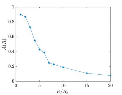
Figure 4: The maximum possible transverse polarization that can be obtained for a positron with the initial conditions mentioned in the text, depending on the bending radius $R$ of the crystal in units of the Tsyganov critical radius $R_{c}$.

$$A=\frac{W_{\uparrow\downarrow}-W_{\downarrow\uparrow}}{W_{\uparrow\downarrow}+W_{\downarrow\uparrow}},$$ (49)

where $W_{fi}$ denotes the total transition rate from state $i$ to state $f$. The quantity $W_{fi}$ for different initial and final spin quantum numbers can be found from Eq. (13) by integrating over angles and photon energies, and by summing over the photon polarization, using a finite piece of trajectory. This formula comes about if it is assumed that the positron has its energy replenished between each radiation emission, as is the case in a synchrotron. With crystals, this would require several thin crystals with accelerating structures in between. We integrated the Lorentz force equation of motion using the electric field obtained from the continuum potential Lindhard (1965); Baier et al. (1998), such that the electric field in the unbent crystal is along the $x$ direction. We then offset the plane along a circular arc in the $xz$ plane, which at the leading order in the small quantity $L/R$, where $L$ is the crystal length, means that the bending follows the curve $x=z^{2}/2R$. One may use this approximation as the total deflection angle $L/R$, is small in a realistic scenario. Due to symmetry, the electric field points along the radius of bending and using Gauss’ law one can show that as long as the distance to the plane is much smaller than the bending radius $R$, the electric field component along the radius of bending is the same as the electric field in the unbent case evaluated at the same distance from the plane. The non-zero components of the electric field are then

$$E_{x}(x,y,z)=E_{\text{cont}}\left(x-\frac{z^{2}}{2R}\right),$$ (50)

$$E_{z}(x,y,z)=-\frac{z}{R}E_{\text{cont}}\left(x-\frac{z^{2}}{2R}\right).$$ (51)

Here, $E_{\text{cont}}(x-z^{2}/2R)$ is the electric field obtained from the continuum potential, in the Doyle-Turner approximation Doyle and Turner (1968); Avakian et al. (1982); Møller (1995), which depends only on the coordinate transverse to the planes (the $x$ coordinate in the considered case). We used a piece of trajectory with roughly 10 periods of oscillation, which was adequate for convergence of the integrals. Moreover, we have integrated over an angular region such that $\boldsymbol{v}_{\bot}(t)$ is contained in the region, with an additional angle of $10/\gamma$ in each direction. This turned out numerically to be sufficient to cover all of the emitted radiation. In Fig. (4) we show the result for a 50 GeV positron with the mentioned initial conditions. It should be mentioned that this maximum polarization is only achievable under the same circumstances as in a storage ring, i.e. a short piece of crystal where radiation occurs, and subsequently a replenishment of the lost energy so that the particles have the nominal energy before entering a crystal again. It is seen that for a strong bending of the crystal, one approaches the value in the constant field of $8/\left(5\sqrt{3}\right)$. While we show only the example of a single trajectory, the method would allow to study radiation reaction in a bent crystal where the effects of polarization of the beam would be essential. We refer the reader to Refs. Wistisen et al. (2018, 2019) for recent experimental studies of radiation reaction in straight crystals.

VI Conclusion

In conclusion we have presented a method to rewrite the semiclassical formulas of Baier, Katkov and Strakhovenko, which facilities their numerical implementation for arbitrary discrete particles quantum numbers. This then allows for the calculation of radiation emission with arbitrary initial and final electron spins, and with arbitrary polarization of the emitted photon when knowing only the classical trajectory of the electron in the background field. In this way, one does not have to know the Dirac wave function in the background field, which is typically an impossible task for realistic field configurations.

First, we have compared the obtained formulas for a case where a solution of the Dirac equation is known, namely the plane-wave field, and find near perfect agreement between the two methods, corroborating the idea that the motion in a plane wave is intrinsically quasiclassical. As an example, we considered the case of the transfer of circular polarization of the radiation, when an electron beam head-on scatters on a short circularly polarized pulse, with the conclusion that the shortness of the pulse implies a slightly lower degree of polarization as compared to the monochromatic-field case. However, much higher degrees of polarization are observed for the photons emitted approximately along the initial direction of propagation of the electrons, in agreement with angular momentum conservation. Finally, we considered the case of a bent crystal and showed how one can calculate the degree of polarization of the positron beam for an arbitrary bending radius of the crystal.

VII Acknowledgements

For T. N. Wistisen this work was supported by the Alexander von Humboldt-Stiftung.

References

- Baier et al. (1998) V.N. Baier, V.M. Katkov, and V.M. Strakhovenko, Electromagnetic Processes at High Energies in Oriented Single Crystals (World Scientific, 1998).
- Belkacem et al. (1985) A. Belkacem, N. Cue, and J.C. Kimball, “Theory of crystal-assisted radiation and pair creation for imperfect alignment,” Phys. Lett. A 111, 86 – 90 (1985).
- Wistisen (2014) T. N. Wistisen, “Interference effect in nonlinear Compton scattering,” Phys. Rev. D 90, 125008 (2014).
- Volkov (1935) D.M. Volkov, “On a class of solutions of the dirac equation,” Z. Phys 94, 250–260 (1935).
- Boca and Florescu (2010) M. Boca and V. Florescu, Rom. J. Phys. 55, 511 (2010).
- Di Piazza (2018) A. Di Piazza, “Completeness and orthonormality of the Volkov states and the Volkov propagator in configuration space,” Phys. Rev. D 97, 056028 (2018).
- Ritus (1985) V.I. Ritus, “Quantum effects of the interaction of elementary particles with an intense electromagnetic field,” Journal of Soviet Laser Research 6, 497–617 (1985).
- Seipt and Kämpfer (2012) D. Seipt and B. Kämpfer, “Two-photon Compton process in pulsed intense laser fields,” Phys. Rev. D 85, 101701 (2012).
- Mackenroth and Di Piazza (2011) F. Mackenroth and A. Di Piazza, “Nonlinear Compton scattering in ultrashort laser pulses,” Phys. Rev. A 83, 032106 (2011).
- Dinu and Torgrimsson (2019) V. Dinu and G. Torgrimsson, “Single and double nonlinear Compton scattering,” Phys. Rev. D 99, 096018 (2019).
- Boca and Florescu (2009) M. Boca and V. Florescu, “Nonlinear Compton scattering with a laser pulse,” Phys. Rev. A 80, 053403 (2009).
- Seipt and Kämpfer (2011) D. Seipt and B. Kämpfer, “Nonlinear Compton scattering of ultrashort intense laser pulses,” Phys. Rev. A 83, 022101 (2011).
- Di Piazza et al. (2012) A. Di Piazza, C. Müller, K. Z. Hatsagortsyan, and C. H. Keitel, “Extremely high-intensity laser interactions with fundamental quantum systems,” Rev. Mod. Phys. 84, 1177–1228 (2012).
- Harvey et al. (2009) C. Harvey, T. Heinzl, and A. Ilderton, “Signatures of high-intensity Compton scattering,” Phys. Rev. A 79, 063407 (2009).
- Hu et al. (2010) H. Hu, C. Müller, and C. H. Keitel, “Complete QED Theory of Multiphoton Trident Pair Production in Strong Laser Fields,” Phys. Rev. Lett. 105, 080401 (2010).
- Meuren et al. (2016) S. Meuren, C. H. Keitel, and A. Di Piazza, “Semiclassical picture for electron-positron photoproduction in strong laser fields,” Phys. Rev. D 93, 085028 (2016).
- Ilderton (2011) Anton Ilderton, “Trident pair production in strong laser pulses,” Phys. Rev. Lett. 106, 020404 (2011).
- Voroshilo et al. (2015) A.I. Voroshilo, S.P. Roshchupkin, and V.N. Nedoreshta, “Parametric interference Compton effect in two pulsed laser waves,” Journal of Physics B: Atomic, Molecular and Optical Physics 48, 055401 (2015).
- Krajewska and Kamiński (2012a) K. Krajewska and J. Z. Kamiński, “Compton process in intense short laser pulses,” Phys. Rev. A 85, 062102 (2012a).
- Krajewska and Kamiński (2012b) K. Krajewska and J. Z. Kamiński, “Breit-Wheeler process in intense short laser pulses,” Phys. Rev. A 86, 052104 (2012b).
- Seipt et al. (2018) D. Seipt, D. Del Sorbo, C. P. Ridgers, and A. G. R. Thomas, “Theory of radiative electron polarization in strong laser fields,” Phys. Rev. A 98, 023417 (2018).
- Angioi et al. (2016) A. Angioi, F. Mackenroth, and A. Di Piazza, “Nonlinear single Compton scattering of an electron wave packet,” Phys. Rev. A 93, 052102 (2016).
- Jackson (1976) J. D. Jackson, “On understanding spin-flip synchrotron radiation and the transverse polarization of electrons in storage rings,” Rev. Mod. Phys. 48, 417–433 (1976).
- Sokolov and Ternov (1966) A.A. Sokolov and I.M. Ternov, “Synchrotron radiation (russian title: Sinkhrotronnoie izluchenie),” Akademia Nauk SSSR, Moskovskoie Obshchestvo Ispytatelei prirody. Sektsia Fiziki. Sinkhrotron Radiation 228, 1 (1966).
- Del Sorbo et al. (2017) D. Del Sorbo, D. Seipt, T. G. Blackburn, A. G. R. Thomas, C. D. Murphy, J. G. Kirk, and C. P. Ridgers, “Spin polarization of electrons by ultraintense lasers,” Phys. Rev. A 96, 043407 (2017).
- Li et al. (2019) Y. F. Li, R. Shaisultanov, K. Z. Hatsagortsyan, F. Wan, C. H. Keitel, and J.X. Li, “Ultrarelativistic electron-beam polarization in single-shot interaction with an ultraintense laser pulse,” Phys. Rev. Lett. 122, 154801 (2019).
- Elishev et al. (1979) A.F. Elishev, N.A. Filatova, V.M. Golovatyuk, I.M. Ivanchenko, R.B. Kadyrov, N.N. Karpenko, V.V. Korenkov, T.S. Nigmanov, V.D. Riabtsov, M.D. Shafranov, B. Sitar, A.E. Senner, B.M. Starchenko, V.A. Sutulin, I.A. Tyapkin, E.N. Tsyganov, D.V. Uralsky, A.S. Vodopianov, A. Forycki, Z. Guzik, J. Wojtkowska, R. Zelazny, I.A. Grishaev, G.D. Kovalenko, B.I. Shramenko, M.D. Bavizhev, N.K. Bulgakov, V.V. Avdeichikov, R.A. Carrigan, T.E. Toohig, W.M. Gibson, Ick-Joh Kim, J. Phelps, and C.R. Sun, “Steering of charged particle trajectories by a bent crystal,” Physics Letters B 88, 387 – 391 (1979).
- Tsyganov (1976) E. N. Tsyganov, “Estimates of cooling and bending processes for charged particle penetration through a mono crystal,” preprint Fermilab TM-684, Batavia USA (1976).
- Jackson (1991) J.D. Jackson, Classical Electrodynamics, 3rd ed. (John Wiley & Sons, Inc., New Jersey, USA, 1991).
- Berestetskii et al. (1971) V.B. Berestetskii, E.M. Lifshitz, and L.P. Pitaevskii, Relativistic Quantum Theory (Elsevier, 1971).
- Note (1) Due to the presence of the finite pulse shape the electric field of the wave is not, rigorously speaking, circularly polarized. For the sake of simplicity, however, in the numerical examples we choose sufficiently long pulses that we can ignore this subtlety.
- Ivanov et al. (2004) D. Yu. Ivanov, G. L. Kotkin, and V. G. Serbo, “Complete description of polarization effects in emission of a photon by an electron in the field of a strong laser wave,” The European Physical Journal C - Particles and Fields 36, 127–145 (2004).
- Di Piazza (2014) A. Di Piazza, “Ultrarelativistic electron states in a general background electromagnetic field,” Phys. Rev. Lett. 113, 040402 (2014).
- Di Piazza (2015) A. Di Piazza, “Analytical tools for investigating strong-field qed processes in tightly focused laser fields,” Phys. Rev. A 91, 042118 (2015).
- Di Piazza (2017) A. Di Piazza, “First-order strong-field QED processes in a tightly focused laser beam,” Phys. Rev. A 95, 032121 (2017).
- Wienands et al. (2015) U. Wienands, T. W. Markiewicz, J. Nelson, R. J. Noble, J. L. Turner, U. I. Uggerhøj, T. N. Wistisen, E. Bagli, L. Bandiera, G. Germogli, V. Guidi, A. Mazzolari, R. Holtzapple, and M. Miller, “Observation of Deflection of a Beam of Multi-GeV Electrons by a Thin Crystal,” Phys. Rev. Lett. 114, 074801 (2015).
- Wistisen et al. (2016) T. N. Wistisen, U. I. Uggerhøj, U. Wienands, T. W. Markiewicz, R. J. Noble, B. C. Benson, T. Smith, E. Bagli, L. Bandiera, G. Germogli, V. Guidi, A. Mazzolari, R. Holtzapple, and S. Tucker, “Channeling, volume reflection, and volume capture study of electrons in a bent silicon crystal,” Phys. Rev. Accel. Beams 19, 071001 (2016).
- Wistisen et al. (2017) T. N. Wistisen, R. E. Mikkelsen, U. I. Uggerhøj, U. Wienands, T. W. Markiewicz, S. Gessner, M. J. Hogan, R. J. Noble, R. Holtzapple, S. Tucker, V. Guidi, A. Mazzolari, E. Bagli, L. Bandiera, and A. Sytov (SLAC E-212 Collaboration), “Observation of quasichanneling oscillations,” Phys. Rev. Lett. 119, 024801 (2017).
- Mazzolari et al. (2014) A. Mazzolari, E. Bagli, L. Bandiera, V. Guidi, H. Backe, W. Lauth, V. Tikhomirov, A. Berra, D. Lietti, M. Prest, E. Vallazza, and D. De Salvador, “Steering of a Sub-GeV Electron Beam through Planar Channeling Enhanced by Rechanneling,” Phys. Rev. Lett. 112, 135503 (2014).
- Baryshevskiĭ and Tikhomirov (1989) V.G. Baryshevskiĭ and V.V. Tikhomirov, “Synchrotron-type radiation processes in crystals and polarization phenomena accompanying them,” Soviet Physics Uspekhi 32, 1013–1032 (1989).
- Baier (1972) V.N. Baier, “Radiative polarization of electrons in storage rings,” Soviet Physics Uspekhi 14, 695–714 (1972).
- Lindhard (1965) J. Lindhard, “Influence of crystal lattice on motion of energetic charged particles,” K. Dan. Vidensk. Selsk. Mat. Fys. Medd. 34, no. 14, 1–64 (1965).
- Doyle and Turner (1968) P. A. Doyle and P. S. Turner, “Relativistic Hartree–Fock X-ray and electron scattering factors,” Acta Crystallogr. A 24, 390–397 (1968).
- Avakian et al. (1982) A.L. Avakian, N.K. Zhevago, and S. Yan, “Emission of electrons and positrons in the axial semichanneling,” J. Exp. Theor. Phys. 82, 573–586 (1982).
- Møller (1995) S.P. Møller, “High-energy channeling - applications in beam bending and extraction,” Nucl. Instrum. Methods Phys. Res. A 361, 403 – 420 (1995).
- Wistisen et al. (2018) T. N. Wistisen, A. Di Piazza, H. V. Knudsen, and U. I. Uggerhøj, “Experimental evidence of quantum radiation reaction in aligned crystals,” Nat. Commun. 9, 795 (2018).
- Wistisen et al. (2019) T. N. Wistisen, A. Di Piazza, C. F. Nielsen, A. H. Sørensen, and U. I. Uggerhøj, “Quantum radiation reaction in aligned crystals beyond the local constant field approximation,” (2019), arXiv:1906.09144 [physics.plasm-ph] .