Dynamic Interference Management for UAV-Assisted Wireless Networks

Abstract

The deployment of unmanned aerial vehicles (UAVs) is proliferating as they are effective, flexible and cost-efficient devices for a variety of applications ranging from natural disaster recovery to delivery of goods. We investigate a transmission mechanism aiming to improve the data rate between a base station (BS) and a user equipment through deploying multiple relaying UAVs. We consider the effect of interference, which is incurred by the nodes of another established communication network. Our primary goal is to design the 3D trajectories and power allocation for the UAVs to maximize the data flow while the interference constraint is met. The UAVs can reconfigure their locations to evade the unintended/intended interference caused by reckless/smart interferers. We also consider the scenario in which smart jammers chase the UAVs to degrade the communication quality. In this case, we investigate the problem from the perspective of both UAV network and smart jammers. An alternating-maximization approach is proposed to address the joint 3D trajectory design and power allocation problem. We handle the 3D trajectory design by resorting to spectral graph theory and subsequently address the power allocation through convex optimization techniques. Finally, we demonstrate the efficacy of our proposed method through simulations.

I Introduction

The utilization of unmanned aerial vehicles (UAVs) has recently become a practical approach for a variety of mission-driven applications including border surveillance, natural disaster aftermath, monitoring, search and rescue, and purchase delivery [2, 3, 4, 5, 6, 7]. Owing to the low acquisition cost of UAVs as well as their fast deployment and efficient coverage capabilities, UAV-assisted wireless communications has attracted extensive interest recently [8, 9, 10, 11, 12, 13, 14]. Specifically, the 3D mobility feature of UAVs and the coexistence of relaying UAVs with other existing communication networks (e.g., cellular networks) have led to new design challenges and opportunities in these networks [15, 16], which are not investigated in the context of classic wireless sensor networks [17]. This fact has promoted an extensive literature dedicated to studying the unique design aspects of these networks, e.g., [18, 19, 20, 21, 22, 23, 24, 25, 26, 27, 28]. In current literature, the UAV-assisted relay communication is mainly studied in two different contexts, in which the network is assumed to be either static, i.e., the positions of the UAVs, transmitter, and receiver are fixed during the data transmission [29, 18, 19, 20, 21, 22], or dynamic [23, 24, 25, 26, 27, 28], where the positions of the transmitter and receiver are assumed to be fixed while the UAVs are typically assumed to be mobile.

In the context of static UAV-assisted wireless communications, in [29], considering an interference limited in band downlink cellular network, the authors studied the effects of scheduling criteria, mobility constraints, path loss models, backhaul constraints, and 3D antenna radiation pattern on trajectory optimization problem of an UAV. In [18], optimal deployment of a UAV in a wireless relay communication system is obtained in order to improve the quality of communications between two obstructed access points by maximizing the average data rate of the system, while limiting the symbol error rate below a threshold. In [19], a relay network is considered in the context of a four node channel setup consisting of a transmitter, a receiver, a UAV relay, and an eavesdropper, where the goal is to shed light on the application of UAV-enabled relaying in secure wireless communications. The secrecy rate maximization problem is formulated, which turns out to be non-convex, for which an iterative approach based on difference of concave (DC) programming is proposed. In [20], the UAVs are utilized to form an aerial backhaul network so as to enhance the performance of the ground network, which is measured through data rate and delay. The link configuration between the UAVs and the gateways, and among the UAVs, is formulated as a network formation game, which is solved through a myopic network formation algorithm. Considering multiple static UAVs, optimal UAV locations are derived in [21] through maximizing the data rate in single link multi-hop and multiple links dual-hop relaying schemes. In this work, it is assumed that the UAVs are hovering at an identical fixed altitude during the transmission. As a follow-up work for [21], in our recent work [22, 30], we studied the optimal position planning of UAV relays between the transmitter and the receiver, which coexist with a major interferer in the environment. In this work, we investigated the following two new problems: i) identifying the minimum required number of UAVs and their optimal positions to satisfy a given SIR of the system, ii) developing a distributed algorithm to maximize the SIR of the system requiring message exchange only between adjacent UAV relays.

In the context of dynamic UAV-assisted wireless communication, in [23], the joint optimization of propulsion and transmission energies for a UAV relay-assisted communication network is studied. A general optimal control problem is formulated for energy minimization based on dynamic models for both transmission and mobility. In [24], the optimum altitude of a UAV for both static and mobile relaying, which corresponds to the circular movements around the user, is considered so as to maximize the reliability of the system, which is measured through total power loss, the overall outage, and the overall bit error rate. It is shown that that decode-and-forward relaying is better than amplify-and-forward relaying in terms of reliability. In [25], a UAV-assisted relay communication network is proposed, where the UAV serves as a relay between a base station and a mobile device. The amplify-and-forward relaying scheme is used, for which the trajectory of UAV, the transmit power of both the UAV and the mobile device are obtained so as to minimize the outage probability of the system. In [26], assuming a source-destination pair and a UAV relay, an end-to-end throughput maximization problem is formulated to optimize the relay trajectory and the source/relay power allocations subject to practical constraints on the UAV speed, transmitting power of the transmitter and the UAV, etc. Afterward, an alternating optimization approach is proposed to jointly derive the optimal transmission power of the transmitter and the UAV, and the UAV trajectory. In [27], a wireless relay network model is considered, in which a fixed-wing UAV serves as a relay among the ground stations with disconnected communication links in the event of disasters. It is assumed that the UAV deploys the decode-and-forward relaying protocol. Considering the fact that in contrast to rotatory-wing UAVs, fixed-wing UAVs require circular movements to maintain their altitude, it is shown that the conventional fixed rate relaying will no longer be effective. To this end, a variable rate relaying approach is proposed to enhance the performance of the system measured through outage probability and information rate. In [28], UAVs are deployed in a wireless network in order to provide connectivity or boost the capacity for the ground users. A nested segmented propagation model is proposed for the air-to-ground channel, based on which they proposed an algorithm to search the optimal UAV position for establishing the best wireless relay link between a base station and a user in a dense urban area.

In this work, we consider the application of UAVs in a more complicated relay network structure, where the network consists of multiple ground/terrestrial nodes and aerial nodes, i.e., UAVs. The direction for the flow of information is assumed to be time varying and thus unknown a priori. In this context, each node is considered to be a transceiver. We aim to propose an analytical framework to enhance the current literature on the subject by incorporating the existence of interferers. We consider the mobility of UAVs during the data transmission to avoid/suppress the interference from multiple interferers.

The existence of multiple interferers in a 3D environment makes our methodology different from the current literature. We pursue two different design schemes considering two different interpretations for the interferers: (i) Reckless interferer and (ii) Smart interferer. Reckless interferers produce interference unintentionally, e.g., primary transmitters in the context of cognitive radio networks. In this case, we study the problem considering two scenarios; First, we assume that the UAV network and the co-existing network (which is referred to as primary network) can cooperate to mitigate the mutual interference; Second, these two networks are assumed to be non-cooperative. We consider both the interference from the primary network to the UAV network and vice versa as the satisfactory performance of both networks is of high importance. Smart interferers, on the other hand, generate interference by intention to interrupt or degrade the communication quality of the UAV network, e.g., mobile jammers, or malicious UAV users. Here, we consider the problem from the perspective of both the UAV network and the smart jammers. In this case, we only consider the interference from the smart jammers to the UAV network. We pursue the problem of joint power allocation and 3D trajectory design for UAVs to maximize the achievable data rate of the network.

I-A Summary of Contributions

• We investigate the UAV-assisted communication problem in the presence of interference based on graph theory. In particular, we formulate the optimization problem as a single commodity maximum flow problem. Considering an interference limited scenario, we deploy a modified signal to interference ratio (SIR) so as to guarantee the safety separation of the UAVs in the 3D trajectory design. We assume different interpretations for the interferers as (i) Reckless interferer (e.g. transmitters in the primary network) and (ii) Smart interferer (e.g. jammers).

• Assuming a reckless interferer, we propose a 3D trajectory design and power allocation scheme in order to improve the transmission flow in the UAV network while an interference constraint is met in the primary network. The 3D trajectory design is addressed using spectral graph theory in which the UAVs try to reconfigure their locations in order to evade the unwanted interference. The power allocation design is done using successive convex approximation (SCA) approach to make sure that the interference constraint on the primary network is satisfied.

• In the case of smart interferers, we approach the problem from both the UAV network and the smart interferers’ perspectives. We propose a 3D trajectory design for the legitimate UAVs in the relay network and the smart interferer. The novel idea for the UAVs in the relay network is to move in a direction to evade the interference caused by the smart interferers. On the other hand, from the smart interferer’s perspective, the smart UAVs aim to chase the legitimate UAVs in the relay network so as to increase the intended interference which leads to degradation of the communication flow between the BS to the user equipment (UE).

The rest of the paper is organized as follows. In Section II, the system model is presented. In Section III, the joint power allocation and 3D trajectory design is formulated and solved for reckless interferer. Section IV presents the formulation and the solution of the maximum flow problem for the case of smart interferers. Simulation results are presented in Section V and finally Section VI concludes the paper.

II System Model

In this section, we will describe the communications scenario and the channel models for the air-to-air (A2A) and air-to-ground (A2G) links.

II-A Communications Scenario

We consider a scenario where a terrestrial BS and a UE aim to engage in communication. The UE is either on the ground (e.g., a moving vehicle, pedestrian) or in the air (e.g., a UAV), as shown in Fig. 1. The channel condition of the direct link between the BS and the UE is not satisfactory for acceptable communication performance due to obstacles located in the line of sight (LoS) area or large distance [31]. To improve the data rate, we consider employing multiple UAVs relaying the signal between the BS and the UE. We also take into account the interference coming from the existing network (e.g., neighboring BSs, small cells, or malicious jammers), and describe the corresponding transmitters as interferers. We term the existing network as the primary network and its UEs as primary UEs. We assume that the interferers can be detected together with their transmission parameters using existing sensing methods in the literature (e.g., [32]). Moreover, we assume that the BS, the UE, the UAVs and the interferers are functioning as both transmitters and receivers, i.e., transceivers, and thus can involve in both uplink and downlink of their own networks. In addition to the communication-related applications, another use case for this scenario is the aerial wireless sensor networks comprised of UAVs equipped with sensors and radio devices, which fly over an area of interest to sense and collect data.

We adopt time-division multiple access (TDMA) to schedule the relaying UAVs so that their transmissions do not collide with each other. Our goal is to obtain the 3D trajectories of the relaying UAVs along with the power allocation to maximize the data rate between the BS and the UE, while the interference constraint on the primary network is met. As we consider a dynamic network, i.e., the nodes can move, designing 3D trajectories is critical since the UAVs should adaptively reconfigure their locations to avoid the interference and transmit their information simultaneously, more than just seeking the final locations to stop and transmit their information. Moreover, 3D trajectory design alone cannot guarantee that the interference threshold constraint is met for the primary network. Thus, a joint 3D trajectory design and power allocation is necessary to address such challenges.

In our setting, $\mathcal{N}$ describes the set of $N$ nodes in our network, which consists of the terrestrial BS (denoted by node $s$), the desired UE (denoted by node $d$), and the relaying UAVs. In addition, $\mathcal{M}$ stands for the set of $M$ separate interferers. The geometric location of any node in the UAV network is denoted by $\textbf{r}_{i}\,{=}\,(x_{i},y_{i},z_{i})\,{\in}\,\mathbb{R}^{3}$ such that $i\,{\in}\,\mathcal{N}$. For the interferer nodes, we have $\textbf{r}^{J}_{m}\,{=}\,(x^{J}_{m},y^{J}_{m},z^{J}_{m})\,{\in}\,\mathbb{R}^{3}$ such that $m\,{\in}\,\mathcal{M}$.

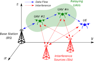
Figure 1: System model for the communications scenario where the desired UE is also a flying UAV. The interferers are assumed as reckless fixed interferers.

II-B A2A and A2G Channel Models

In this section, we discuss the A2A and the A2G channel models under consideration. In this work, we consider transmission through the line-of-sight (LoS) path only (e.g., [21]), and adopt a widely-used path-loss model provided by the International Telecommunication Union (ITU). The path-loss for the A2A link is therefore given (in dB scale) as

$$\textrm{PL}^{\textrm{A2A}}_{\textrm{dB}}(d_{i,j})=\alpha_{1}10\log_{10}d_{i,j}+\eta_{1},$$ (1)

where $\alpha_{1}$ is the path-loss exponent, $d_{i,j}$ is the Euclidean distance between the UAVs $i$ and $j$, and $\eta_{1}$ is the path loss associated with the reference LoS distance of $1\,\text{m}$. Similarly, the A2G channel between any terrestrial node and the aerial node can be described by the path-loss expression given by

$$\textrm{PL}^{\textrm{A2G}}_{\textrm{dB}}(d_{i,j})=\alpha_{2}10\log_{10}d_{i,j}+\eta_{2},$$ (2)

where $\alpha_{2}$ is the path-loss exponent, and $\eta_{2}$ is the path-loss at the reference distance. Note that in the free space, the path-loss exponents would be $\alpha_{\ell}\,{=}\,2$, and the path-loss at the reference distance would become $\eta_{\ell}\,{=}\,10\log_{10}\,(\frac{4\pi f_{\rm c}}{c})^{2}$, where $f_{\rm c}$ is the carrier frequency, $c\,{=}\,3\times 10^{8}\,\text{m/s}$ is the speed of light, and $\ell\,{\in}\,\{1,2\}$. As in [33], we consider a larger path-loss exponent for the A2G channels compared to the A2A channels, where these parameters are presented in Section V. Considering the impact of small-scale fading, the overall complex channel gain for nodes $i$ and $j$ involved in either the A2A or A2G communications becomes

$$h_{i,j}=\begin{cases}\displaystyle\frac{g_{i,j}}{\sqrt{\textrm{PL}^{\textrm{A2A}}(d_{i,j})}},&\textrm{if the link is A2A},\\ \displaystyle\frac{g_{i,j}}{\sqrt{\textrm{PL}^{\textrm{A2G}}(d_{i,j})}},&\textrm{if the link is A2G},\end{cases}$$ (3)

where $g_{i,j}$ is the small-scale fading gain, which is a zero-mean complex Gaussian random variable with unit variance. As a final remark, we assume perfect channel reciprocity for all the links under consideration so that the link $(i,j)$ from the node $i$ to node $j$ is equivalent to the link $(j,i)$ in the opposite direction.

II-C Graph Representation of the Network

We assume that the interference coming from the interferers is much stronger than the noise. We therefore take into account the SIR as the performance metric, which is defined at node $j$ for the transmission from node $i$ as follows:

$$\textrm{SIR}_{i,j}=\frac{P_{i}\,|h_{i,j}|^{2}}{\sum\limits_{m\in\mathcal{M}}{P}_{m}^{\textrm{J}}\,|h_{m,j}|^{2}+\chi\sum\limits_{k\in{\mathcal{Q}}_{i,j}}u(d_{j,k}/r_{\textrm{int}})},$$ (4)

where $\mathcal{Q}_{i,j}\,{=}\,\mathcal{N}\,{\backslash}\,\{i,j\}$, $P_{i}$ is the transmit power of UAV $i$ in the UAV network. and ${P}_{m}^{\textrm{J}}$ is the transmit power of interferer $m$ in the primary network (i.e., $m\,{\in}\,\mathcal{M}$). Let us define $\mathbf{P}=[P_{1},...,P_{N}]$ and $\mathbf{P}^{J}=[P_{1}^{J},...,P_{M}^{J}]$ in vector forms as well. The second term in the denominator of (4) is considered to guarantee a safety separation between any of the UAVs and other nodes in the UAV network (i.e., the BS, the desired UE, or the other UAVs) so as to preserve a proper flight performance [34]. In this representation, $\chi$ stands for the importance of this safety precaution, and $u$ is the smoothed step function given by [35]:

$$u(y)=\zeta\frac{\textrm{exp}(-\kappa y-\log y_{0})}{1+\textrm{exp}(-\kappa y-\log y_{0})},$$ (5)

where $y_{0}$ is an arbitrarily small positive number, and $\zeta$ and $\kappa$ are design parameters. We first define a directed flow graph $G\,{=}\,(\mathcal{N},\mathcal{E})$, in which $\mathcal{E}$ denotes the set of available edges in the network and each edge has the capacity $a_{i,j}$. We assume a line topology for the multi-hop relay network [21]. This is a reasonable assumption as the major information exchange happens between neighboring UAVs, not between the UAVs away by more than a single hop. We formulate the information exchange in this single-source and single-destination network as a single-commodity maximum flow problem, for which the task is to determine the maximum amount of flow, i.e., the maximum average transmission rate, between the BS and the desired UE.

The average transmission rate is defined as the arithmetic mean of the data rates in the forward and backward directions for each pair of nodes. The generalized adjacency matrix is accordingly defined as $\mathbf{A}\,{=}\,[a_{i,j}]_{\{i,j\}{=}1}^{N}$, where $a_{i,j}$ is the average transmission rate between nodes $i$ and $j$, given by:

$$a_{i,j}=\begin{cases}\frac{1}{2}{B}\Big{(}{\log_{2}(1{+}\textrm{SIR}_{i,j})}{+}{\log_{2}(1{+}\textrm{SIR}_{j,i})}\Big{)},&i{\neq}j,\\ 0,&i{=}j,\end{cases}$$ (6)

with ${B}$ the transmission bandwidth of the network. Note that $\textrm{SIR}_{i,j}$ is, in general, not equal to $\textrm{SIR}_{j,i}$, in part, due to the unbalanced deployment of interferer. We further define the generalized degree matrix of the network as $\mathbf{D}=\textrm{diag}\{\beta_{1},...,\beta_{N}\}$, where $\beta_{i}=\sum_{\{j|j\neq i\}}a_{i,j}$. Finally, the Laplacian matrix of the network graph is given by $\mathbf{L}\,{=}\,\mathbf{D}\,{-}\,\mathbf{A}$.

In the following two sections, we formulate the 3D trajectory and power allocation problem introduced in Section under two different types of interference source. In particular, we consider reckless and smart (i.e., intended) interferers in sequence, and propose a solution to the problem for each of these scnarios.

III Reckless Interferer

We first consider the reckless interference for which the primary role of the interferer is not to produce interference in our UAV-assisted network on purpose, but rather to transmit message signal to its desired UEs, as shown in Fig. 1. This type of interference is mainly caused by the transmitters within the existing network (e.g., neighbouring BSs, small cells), and hence is reckless. This type of interferer might be static or mobile, and its location is known to the UAVs. Note that any mobile interferer of this type is not moving intelligently so as to impair the communications in the UAV-assisted network.

In this scenario, since we assume that the UAVs are working in an already existing network, they must satisfy the interference constraint at primary receivers located on the ground. Thus, we need a constraint on the transmitted signal from the UAVs. On other other hand, for a reliable communication of the primary nodes, they need some order of protection as well. We assume that the interferers (which can serve as BSs in primary network) are serving a set of primary UEs. We denote the set of all primary UEs in the primary network by $\mathcal{R}$, where their locations are given by $\textbf{r}^{\mathcal{R}}_{u}\,{=}\,(x_{u},y_{u},z_{u})\,{\in}\,\mathbb{R}^{3}$ with $u\,{\in}\,\mathcal{R}$. Since the interferers in the reckless case can be assumed as co-existing BSs, we should guarantee that the quality of service (QoS) of its users is satisfied. The interferers can either cooperate with the UAV network or not. In the case of cooperation, the primary network can adjust its transmission power to avoid generating excessive interference to the UAV network while satisfying its own user’s QoS. In the absence of cooperation, the interferer in the primary network is not capable of adjusting its transmit power. We assume that the SINR at primary UEs on the ground is affected by the UAVs interference. The SINR at each UE $u\in\mathcal{R}$ from the transmitter $m\in\mathcal{M}$ while UAV $i$ transmits at the same time is given by

$$\textrm{SINR}_{m,u}=\frac{P_{m}^{J}\,|h_{m,u}|^{2}}{{P}_{i}\,|h_{i,u}|^{2}+\sigma^{2}},$$ (7)

where $\sigma^{2}$ is the noise variance and the first term in the denominator is the interference from the UAV transmitting at the corresponding time slot. The associated rate between the primary UE $u$ and interferer $m$ while the UAV $i$ is transmitting at the same time can therefore be obtained by $R_{m,u}(P_{i},P_{m}^{J})=B\log_{2}(1+\textrm{SINR}_{m,u})$. In order to guarantee the quality of service of the primary UEs, their transmission rates should be larger than a predefined threshold $R^{\rm{th}}$. Considering this assumption, if two networks cooperate, we can adjust the transmit power of the primary network as well to avoid producing more interference while the QoS of its network is guaranteed. In real scenarios, this assumption might not be able to be satisfied properly; however, it can provide some insights on the upper bound of the performance of the UAV network.

III-A Optimization Problem Formulation

Here, we formulate the optimization problem for the overall network, where the goal is to maximize the data flow $\textrm{R}_{\textrm{s}\leftrightarrow\textrm{d}}$ between the terrestrial BS and the desired UE with the help of relaying UAVs in the presence of interferers. The flow of the network can be assumed as a measure of average uplink/downlink transmission capability of the UAV network. For each link $(i,j)\,{\in}\,\mathcal{E}$, let $f_{i,j}$ be the associated flow such that $0\,{\leq}\,f_{i,j}\,{\leq}\,a_{i,j}$. The desired optimization problem is therefore given as follows:

$$\max_{\begin{subarray}{c}P_{i},\textbf{r}_{i}\forall i\in\mathcal{Q}_{s,d}\\ {P}_{m}^{\textrm{J}},\forall m\in\mathcal{M}\end{subarray}} \qquad\textrm{R}_{\textrm{s}\leftrightarrow\textrm{d}}\;\,{=}\,\!\!\!\sum\limits_{j:(s,j)\in\mathcal{E}}f_{s,j}$$ (8)

s.t. $$\!\!\!\sum\limits_{i:(i,j)\in\mathcal{E}}f_{i,j}-\!\!\!\sum\limits_{l:(j,l)\in\mathcal{E}}f_{j,l}\,{=}\,0,\;\forall j\in\mathcal{Q}_{s,d},$$ (9a)

$$0\leq f_{i,j}\leq a_{i,j},~{}\forall(i,j)\in\mathcal{E},$$ (10a)

$$P_{i}|h_{i,m}|^{2}\leq\textrm{I}^{\textrm{max}}_{m},\;\forall i\in\mathcal{N},m\in\mathcal{M},$$ (11a)

$$P_{i}\leq\textrm{P}_{\textrm{max}},\;\forall i\in\mathcal{N},$$ (12a)

$$R^{{\rm th}}\leq R^{i}_{u,m}(P_{i},P_{m}^{J}),~{}\forall m\in\mathcal{M},u\in\mathcal{R},i\in\mathcal{N},~{}~{}$$ (13a)

where $P_{i}$ stands for the power of the $i$th UAV, $\textrm{P}_{\textrm{max}}$ is the maximum transmit power of each UAV, and $\textrm{I}^{\textrm{max}}_{m}$ represents the predefined interference threshold for the $m$-th interferer. In addition, (9a) is due to the assumption of balanced flows for all the nodes except the source and the destination. Constraint (10a) ensures that the flow of each link is less than the maximum capacity. Moreover, (11a) satisfies the condition that the interference produced by each UAV at any interferer is always less than a predefined threshold $\textrm{I}^{\textrm{max}}_{m}$ for the $m$-th interferer. This can guarantee the performance of the primary network in uplink scenario. Constraint $\eqref{eqn:joint_opt_5}$ is imposed to limit the transmission power of the UAVs. Constraint (13a) is a QoS service consideration for the UEs in the primary network which guarantees the QoS of the primary users in downlink. By imposing this condition and adjusting the transmission power of the primary network interferers, the primary network stops generating stronger interference while satisfying the QoS constraints.

It is worth mentioning that given the UAVs’ transmission powers, there is no guarantee that the interference constraint is met at the co-existing primary network with the 3D trajectory design solely [36]. On the other hand, assuming fixed locations for UAVs, solely optimizing the UAV transmission powers leads to a poor performance at the UAV relay network. Thus, joint power allocation and 3D trajectory design is necessary to obtain the satisfactory performance for both networks, and it is therefore very complicated to obtain the optimal trajectory and UAVs’ transmit powers. In the following, we deploy to decompose the overall optimization of (8) into two sub-problems using the alternating-optimization approach [37]. In the proposed strategy, we first solve the problem of 3D trajectory optimization for a given set of transmit powers (i.e., $P_{i},\forall i\in\mathcal{N}$), and then the power allocation problem is solved for the given set of UAV locations computed beforehand. These recursions continue till a satisfactory level of performance is obtained.

III-B 3D Trajectory Optimization

We first attempt to solve the optimization problem in (8) to obtain 3D trajectories of the UAVs assuming an initial set of transmit power values is given. The optimization therefore reduces to a maximum flow problem with respect to the locations, which is given as

$$\max_{\begin{subarray}{c}\textbf{r}_{i}\\ \forall i\in\mathcal{Q}_{s,d}\end{subarray}} \qquad\textrm{R}_{\textrm{s}\leftrightarrow\textrm{d}}\;\,{=}\,\!\!\!\sum\limits_{j:(s,j)\in\mathcal{E}}f_{s,j}$$ (14)

s.t. $$\qquad\eqref{eqn:joint_opt_2},\eqref{eqn:joint_opt_3}.$$

Note that the maximum flow problem in (14) can be solved for a given UAV location using the well-known max-flow-min-cut theorem [38]. The achievable maximum flow of the network is equal to single flow min-cut of the underlying network given by

$$\textrm{R}^{\textrm{max}}_{\textrm{s}\leftrightarrow\textrm{d}}=\min_{\begin{subarray}{c}\{S:v_{s}\in S,v_{d}\in\bar{S}\}\end{subarray}}\sum\limits_{i\in S,j\in\bar{S}}a_{i,j}.$$ (15)

The maximum flow in (15) can be obtained by the Ford-Fulkerson algorithm [38]. The challenging task is to design the trajectories (i.e., moving directions) of each UAV in the 3D space so as to maximize the information flow between the BS and the desired UE.

In order to move towards the maximum flow trajectory, we use Cheeger constant or isoperimetric number of the graph, which provides numerical measure on how well-connected our multi-node primary wireless network is [39]. Assuming that $\mathcal{L}\,{=}\,\mathbf{D}^{-1/2}\mathbf{L}\mathbf{D}^{-1/2}$ is the normalized Laplacian matrix, the Cheeger constant is given as [39]

$$h(\mathcal{L})=\underset{S}{\text{min}}\frac{\sum_{i\in S,j\in\bar{S}}a_{i,j}}{\text{min}\{|S|,(|\bar{S}|)\}},$$ (16)

where $S\,{\subset}\,\mathcal{N}$ is a subset of the nodes, $\bar{S}\,{=}\,\mathcal{N}\,{-}\,S$, and $|S|$ is the cardinality of set $S$.

Note that the original definition of the Cheeger constant $h(\mathcal{L})$ considers all the nodes in the network with equal importance. Since the maximum flow of the network for a given source-destination pair depends on the individual link capacities, the weighted version of the Cheeger constant appears as a promising solution to overcome this drawback. In particular, the original Cheeger constant blindly aims at improving the weakest link in the network and may fail to emphasize the desired flow associated with a particular source-destination pair. We therefore need to distinguish between the BS and the desired UE from the UAV nodes, for which the weighted Cheeger constant comes as a remedy, and is given as [35]

$$h_{\mathbf{W}}(\mathcal{L})=\underset{S}{\text{min}}\frac{\sum_{i\in S,j\in\bar{S}}a_{i,j}}{\text{min}\{|S|_{\mathbf{W}}),(|\bar{S}|_{\mathbf{W}})\}},$$ (17)

where $|S|_{\mathbf{W}}\,{=}\,\sum_{i\in S}w_{i}$ is the weighted cardinality, and $w_{i}\,{\geq}\,0$ is the weight of the node $i$ which is adopted to emphasize any bottleneck along the flow from the BS to the desired UE. The weighted Laplacian matrix is accordingly given by

$$\mathcal{L}_{\mathbf{W}}=\mathbf{W}^{-1/2}\mathcal{L}\mathbf{W}^{-1/2},$$ (18)

where $\mathbf{W}\,{=}\,{\rm diag}\{w_{1},...,w_{n}\}$. Usually, the Cheeger constant is difficult to compute. To address this issue, algebraic connectivity can be considered as a suitable alternative. The weighted second smallest eigenvalue $\lambda_{2}({\mathcal{L}_{\mathbf{W}}})$ can be defined as

$$\lambda_{2}(\mathcal{L}_{\mathbf{W}})=\underset{\textbf{v}\neq\textbf{0},\textbf{v}\perp\mathbf{W}^{1/2}\textbf{1}}{\text{min}}\frac{\langle\mathcal{L}_{\mathbf{W}}\textbf{v},\textbf{v}\rangle}{\langle\textbf{v},\textbf{v}\rangle}.$$ (19)

It is shown in [35] that the following weighted Cheeger’s inequalities hold

$$\lambda_{2}(\mathcal{L}_{\mathbf{W}})/2\leq h_{\mathbf{W}}(\mathcal{L}_{\mathbf{W}})\leq\sqrt{2\delta_{\textrm{max}}\lambda_{2}(\mathcal{L}_{\mathbf{W}})/w_{\textrm{min}}}\,,$$ (20)

where $\delta_{\textrm{max}}$ is the maximum node degree, and $w_{\textrm{min}}=\min_{i}w_{i}$. As can be seen, when $\lambda_{2}(\mathcal{L}_{\mathbf{W}})$ gets larger values, the lower bound of the weighted Cheeger constant increases, which improves the connectivity of the overall network, and suppresses the formation of bottleneck. The UAVs can therefore adjust their geometric locations in order to maximize $\lambda_{2}({\mathcal{L}_{\mathbf{W}}})$, and hence $h_{\mathbf{W}}(\mathcal{L})$.

As a result, each UAV should move along the spatial gradient of the weighted algebraic connectivity $\lambda_{2}({\mathcal{L}_{\mathbf{W}}})$ to maximize it. Given the instantaneous location of the $i$th UAV, its spatial gradient along $x$-axis is given as follows:

$$\frac{\partial\lambda_{2}({\mathcal{L}_{\mathbf{W}}})}{\partial x_{i}} ={\mathbf{x}^{f}}^{T}\frac{\partial({{\mathcal{L}_{\mathbf{W}}}})}{\partial x_{i}}{\mathbf{x}^{f}}=\sum_{p=1}^{N}\sum_{q=1}^{N}\frac{v_{p}^{f}}{\sqrt{w_{p}}}\frac{v_{q}^{f}}{\sqrt{w_{q}}}\left[\frac{\partial\mathcal{L}}{\partial x_{i}}\right]_{p,q}$$ (21)

$$=\sum_{\{p,q:p\sim q\}}\left[\frac{v_{p}^{f}}{\sqrt{w_{p}}}-\frac{v_{q}^{f}}{\sqrt{w_{q}}}\right]^{2}\frac{\partial a_{p,q}}{\partial x_{i}},$$ (22)

where ${v}^{f}_{k}$ is the $k$th entry of $\mathbf{v}^{f}$ with $k\,{\in}\,\{p,q\}$, $\mathbf{v}^{f}$ is the Fiedler vector which is the eigenvector corresponding to the second smallest eigenvalue $\lambda_{2}({\mathcal{L}_{\mathbf{W}}})$, and $p\,{\sim}\,q$ means that the nodes $p$ and $q$ are connected. In (22), $\frac{\partial a_{p,q}}{\partial x_{i}}$ can be computed as

$$\frac{\partial a_{p,q}}{\partial x_{i}} =\textrm{B}\left[\frac{1}{1{+}\textrm{SIR}_{p,q}}\frac{\partial\textrm{SIR}_{p,q}}{\partial x_{i}}+\frac{1}{1{+}\textrm{SIR}_{q,p}}\frac{\partial\textrm{SIR}_{q,p}}{\partial x_{i}}\right],$$ (23)

which is $0$ for $p\,{=}\,q$, or $i\,{\notin}\,\{p,q\}$. The partial derivative of SIR with respect to $x_{i}$ in (23) can be computed using (4) together with the geometrical relations between $x_{i}$ and the complex channel gain $h_{i,j}$ presented in Section II. Assuming $p\,{=}\,i$ and $p\neq q$, we have

$$\frac{\partial\textrm{SIR}_{i,q}}{\partial x_{i}}=\frac{10^{-\eta_{l}/10}|g_{i,q}|^{2}\alpha_{l}d_{i,q}^{-\alpha_{l}-2}(x_{q}-x_{i})}{{\sum\limits_{m\in\mathcal{M}}{P}_{m}^{\textrm{J}}\,|h_{q,m}|^{2}+\chi\sum\limits_{k\in{\mathcal{Q}}_{i,j}}u(d_{q,k}/r_{\textrm{int}})}},$$ (24)

and

$$\frac{\partial\textrm{SIR}_{q,i}}{\partial x_{i}}= \frac{10^{-\eta_{l}/10}|g_{i,q}|^{2}\alpha_{l}d_{i,q}^{-\alpha_{l}-2}(x_{q}-x_{i})}{\Big{(}{\sum\limits_{m\in\mathcal{M}}{P}_{m}^{\textrm{J}}\,|h_{i,m}|^{2}+\chi\sum\limits_{k\in{\mathcal{Q}}_{i,j}}u(d_{i,k}/r_{\textrm{int}})}\Big{)}}$$

$$+ \frac{d^{-\alpha_{l}}_{i,m}10^{-\eta_{l}/10}\sum\limits_{m\in\mathcal{M}}|g_{i,m}|^{2}\alpha_{l}d_{i,m}^{-\alpha_{l}-2}(x_{i}-x_{m})}{\Big{(}{\sum\limits_{m\in\mathcal{M}}{P}_{m}^{\textrm{J}}\,|h_{i,m}|^{2}+\chi\sum\limits_{k\in{\mathcal{Q}}_{i,j}}u(d_{i,k}/r_{\textrm{int}})}\Big{)}^{2}}$$

$$+ \frac{d^{-\alpha_{l}}_{i,m}10^{-\eta_{l}/10}\sum\limits_{k\in{\mathcal{Q}}_{i,j}}u^{{}^{\prime}}(d_{i,k}/r_{\textrm{int}})\frac{x_{k}-x_{i}}{r_{\textrm{int}}d_{i,k}}}{\Big{(}{\sum\limits_{m\in\mathcal{M}}{P}_{m}^{\textrm{J}}\,|h_{i,m}|^{2}+\chi\sum\limits_{k\in{\mathcal{Q}}_{i,j}}u(d_{i,k}/r_{\textrm{int}})}\Big{)}^{2}},$$ (25)

where $u^{{}^{\prime}}(x)\,{=}\,{\rm{d}}u/{\rm{d}}x$. If $i\,{\notin}\,\{p,q\}$ and $p\,{\neq}\,q$, one can obtain

$$\frac{\partial\textrm{SIR}_{p,q}}{\partial x_{i}}= \frac{u^{{}^{\prime}}(d_{q,i}/r_{\textrm{int}})}{\Big{(}{\sum\limits_{m\in\mathcal{M}}{P}_{m}^{\textrm{J}}\,|h_{q,m}|^{2}+\chi\sum\limits_{k\in{\mathcal{Q}}_{i,j}}u(d_{q,k}/r_{\textrm{int}})}\Big{)}^{2}}\frac{x_{i}-x_{q}}{r_{\textrm{int}}d_{q,i}},$$ (26)

and ${\partial\textrm{SIR}_{q,p}}/{\partial x_{i}}$ can be obtained similar to (26) by changing the subscripts $p$ and $q$. The update in the location of the $i$th UAV along the $x-$axis is then given as

$$x_{i}(t+1)=x_{i}(t)+{\rm d}t\frac{\partial\lambda_{2}({\mathcal{L}_{\mathbf{W}}})}{\partial x_{i}(t)},$$ (27)

where $t$ stands for the discrete time, or, equivalently, the iteration number. A similar procedure can be pursued to find the spatial gradients of $\lambda_{2}({\mathcal{L}_{\mathbf{W}}})$ along the $y-$ and $z-$axis, and update the coordinates.

III-C Power Allocation Optimization

We now focus on the power allocation problem, and solve the optimization problem in (8) to find the optimal power allocation for a given set of the UAV locations. In this case, we consider the reckless interferer generating the unwanted interference. Here, we assume that the primary network and the UAV network can cooperate so as to mitigate the mutual interference. The UAVs try to mitigate the mutual unwanted interference between the primary co-existing network and the UAV network in order to improve their information flow between the source and the destination. However, 3D trajectory design solely can not guarantee that the interference threshold is met in the primary network. Thus, the power allocation should be done in order to guarantee the interference threshold constraint. The corresponding optimization becomes

$$\max_{\begin{subarray}{c}P_{i}\forall i\in\mathcal{Q}_{s,d}\\ {P}_{m}^{\textrm{J}},\forall m\in\mathcal{M}\end{subarray}} \qquad\textrm{R}_{\textrm{s}\leftrightarrow\textrm{d}}\;\,{=}\,\!\!\!\sum\limits_{j:(s,j)\in\mathcal{E}}f_{s,j}$$ (28)

s.t. $$\qquad\!\eqref{eqn:joint_opt_2},\eqref{eqn:joint_opt_3},\eqref{eqn:joint_opt_4},\eqref{eqn:joint_opt_5},\eqref{eqn:joint_opt_6}.$$

In this case, the maximum information exchange of the network is determined by the link with the minimum instantaneous rate. Hence, as we try to maximize the flow of the network, we equivalently maximize the information exchange of the hop with the minimum instantaneous rate. More specifically, the power allocation problem can be equivalently given by

$$\max_{\begin{subarray}{c}P_{i}\forall i\in\mathcal{Q}_{s,d}\\ {P}_{m}^{\textrm{J}},\forall m\in\mathcal{M}\end{subarray}}\;\min_{\begin{subarray}{c}\forall\,j\in\mathcal{Q}_{s,d}\end{subarray}} \qquad a_{i,j}$$ (29)

s.t. $$\qquad\eqref{eqn:joint_opt_4},\eqref{eqn:joint_opt_5},\eqref{eqn:joint_opt_6}.$$

In order to have a more tractable problem, (29) can be reformulated as follows:

$$\max_{\begin{subarray}{c}P_{i}\forall i\in\mathcal{Q}_{s,d}\\ {P}_{m}^{\textrm{J}},\forall m\in\mathcal{M}\end{subarray}} \qquad\eta$$ (30)

s.t. $$\qquad 0\leq\eta\leq a_{i,j},\,\forall j\in\mathcal{Q}_{s,d},$$

$$\qquad\eqref{eqn:joint_opt_4},\eqref{eqn:joint_opt_5},\eqref{eqn:joint_opt_6},$$

where $\eta$ is an auxiliary variable employed to facilitate the optimization. In this case, the objective is an affine function. However, the constraint on $a_{i,j}$ is not convex. $a_{i,j},$ $\forall\,i,j\in\mathcal{Q}_{s,d}$, can be recast as the difference of two concave functions, given by $a_{i,j}(P_{i},P_{j},\mathbf{P}^{J})=v(P_{i},P_{j},\mathbf{P}^{J})-r(\mathbf{P}^{J})$, where

$$v(P_{i},P_{j},\mathbf{P}^{J})=$$

$$\frac{1}{2}B\log_{2}\left({P_{i}\,|h_{i,j}|^{2}}+{\sum\limits_{m\in\mathcal{M}}{P}_{m}^{\textrm{J}}\,|h_{m,j}|^{2}+\chi\sum\limits_{k\in{\mathcal{Q}}_{i,j}}u(d_{j,k}/r_{\textrm{int}})}\right)+$$

$$\frac{1}{2}B\log_{2}\left({P_{j}\,|h_{j,i}|^{2}}+{\sum\limits_{m\in\mathcal{M}}{P}_{m}^{\textrm{J}}\,|h_{m,i}|^{2}+\chi\sum\limits_{k\in{\mathcal{Q}}_{i,j}}u(d_{i,k}/r_{\textrm{int}})}\right),$$ (32)

and

$$r(\mathbf{P}^{J})= \frac{1}{2}B\log_{2}\Big{(}{\sum\limits_{m\in\mathcal{M}}{P}_{m}^{\textrm{J}}\,|h_{m,j}|^{2}+\chi\sum\limits_{k\in{\mathcal{Q}}_{i,j}}u(d_{j,k}/r_{\textrm{int}})}\Big{)}$$

$$+ \frac{1}{2}B\log_{2}\Big{(}{\sum\limits_{m\in\mathcal{M}}{P}_{m}^{\textrm{J}}\,|h_{m,i}|^{2}+\chi\sum\limits_{k\in{\mathcal{Q}}_{i,j}}u(d_{i,k}/r_{\textrm{int}})}\Big{)}.$$ (33)

Algorithm 1 DC-based SCA Algorithm for Power Allocation

1:Initialization: Iteration number $t:=1$, locations $\textbf{r}_{i}$ $,\forall i\in\mathcal{N}$, feasible initial value for $P_{i}[0],~{}\forall i\in\mathcal{N}$ and $\mathbf{P}^{J}{[0]}$.

2:Calculate the value of $\tilde{a}_{i,j}(P_{i}[0],P_{j}[0],\mathbf{P}^{J}[0])$, $\forall i\in\mathcal{N}$ using (35).

3:while $|\eta[t]\,{-}\,\eta[t-1]|\,{>}\,\varepsilon$  do

4:     Compute the optimal power allocation $P_{i}[t],~{}\forall i\in\mathcal{N}$ and $\mathbf{P}^{J}{[t]}$ in (36) using CVX [40].

5:     Compute $\tilde{a}_{i,j}(P_{i}[t],P_{j}[t],\mathbf{P}^{J}[t])$, $\forall i\in\mathcal{N}$ using (35).

6:     $t\leftarrow t+1$

7:end while

In general, the difference of two concave functions is not a concave one [41]. In order to convexify this function at iteration $t$, we deploy first-order Taylor expansion to approximate $r(\mathbf{P}^{J})$ around a given point from the previous iteration $\mathbf{P}^{J}[t-1]$ as:

$$\tilde{r}(\mathbf{P}^{J})\approx r(\mathbf{P}^{J}[t-1])+(\nabla r(\mathbf{P}^{J}[t-1]))^{T}(\mathbf{P}^{J}-\mathbf{P}^{J}[t-1]).$$ (34)

Thus, we have the approximated version of $a_{i,j}(P_{i},P_{j},\mathbf{P}^{J})$ as

$$\tilde{a}_{i,j}(P_{i},P_{j},\mathbf{P}^{J})=v(P_{i},P_{j},\mathbf{P}^{J})-\tilde{r}(\mathbf{P}^{J}).$$ (35)

Using this approximation, one can see that $\tilde{a}_{i,j}(P_{i},P_{j},\mathbf{P}^{J})$ is a concave function. A similar approximation can be adopted for the constraint $\eqref{eqn:joint_opt_6}$ to make it convex as a new constraint ($\hat{\textrm{8e}}$). To do this, we can re-write the constraint $\eqref{eqn:joint_opt_6}$ as: Thus, the optimization problem in (30) can be recast as:

$$\max_{\begin{subarray}{c}P_{i}\forall i\in\mathcal{Q}_{s,d}\\ {P}_{m}^{\textrm{J}},\forall m\in\mathcal{M}\end{subarray}} \qquad\eta$$ (36)

s.t. $$\qquad 0\leq\eta\leq\tilde{a}_{i,j},\,\forall j\in\mathcal{Q}_{s,d},$$

$$\qquad\eqref{eqn:joint_opt_4},\eqref{eqn:joint_opt_5},(\hat{\textrm{8e}}).$$

After substituting the approximated versions of the constraints, in each iteration $l$, the above optimization problem is now convex, which can be solved efficiently using the interior point method [42]. This procedure, called successive convex approximation (SCA) [43], is described in Algorithm 1.

Proposition 1

Algorithm 1 generates a sequence of improved feasible points that converge to a point $(\mathbf{P}^{*},\mathbf{P}^{J*})$ satisfying the KKT conditions of the problem (30).

Proof

The proof is omitted due to brevity. Similar proof can be found in [44].

If the primary network does not cooperate with UAV network to adjust its transmission power so as to help improve the UAV transmission flow, the optimization can be done with respect to the UAVs’ transmit powers while the transmit powers of the existing network are fixed.

III-D The Joint Alternating-Optimization Algorithm

Given the transmit powers of the UAVs, the trajectory design problem can be solved based on the Cheeger constant in Section III-B. Given the locations of the UAVs, the power allocation can be obtained using the SCA method as in Algorithm 1 discussed in Section III-C. At each step of 3D trajectory design, we need to make sure that the interference threshold constraint is met in the primary network. Thus, at each iteration of 3D trajectory design, we compute new set of transmit powers for UAVs. The overall algorithm considering both the 3D trajectory and power allocation optimization is summarized in Algorithm 2.

Algorithm 2 Proposed Alternating-Optimization Algorithm

Initialization: Locations $\textbf{r}_{i}$ and power allocation $P_{i}$ for $i$th UAV for $\forall i\,{\in}\,\mathcal{N}\,{\cup}\,\mathcal{M}$, error tolerance $\varepsilon$

$t\leftarrow 1$, $\textrm{R}_{\textrm{s}\leftrightarrow\textrm{d}}({-}1)\leftarrow{-}\infty$, $\textrm{R}_{\textrm{s}\leftrightarrow\textrm{d}}(0)\leftarrow 0$

while  $|\textrm{R}_{\textrm{s}\leftrightarrow\textrm{d}}(t{-}1)\,{-}\,\textrm{R}_{\textrm{s}\leftrightarrow\textrm{d}}(t{-}2)|\,{>}\,\varepsilon$  do

     Compute $\frac{\partial\lambda_{2}({\mathcal{L}_{\mathbf{W}}})}{\partial x_{i}(t)}$, $\frac{\partial\lambda_{2}({\mathcal{L}_{\mathbf{W}}})}{\partial y_{i}(t)}$, $\frac{\partial\lambda_{2}({\mathcal{L}_{\mathbf{W}}})}{\partial z_{i}(t)}$ by (41)-(23)

     Update $\textbf{r}_{i}(t)$ in $\mathbb{R}^{3}$ as in (27)

     Compute optimal $\mathbf{P}$ and $\mathbf{P}^{J}$ using SCA algorithm given in Algorithm 1.

     Compute $\textrm{R}_{\textrm{s}\leftrightarrow\textrm{d}}(t)$ by Ford-Fulkerson algorithm [38]

     $t\leftarrow t+1$

end while

IV Smart Interferer

In this scenario, we assume that interferers are smart, as shown in Fig. 2. Smart interferers can move in order to decrease the flow of the UAV network. The moving smart interferers can be assumed as other UAVs trying to interrupt or at least degrade the quality of the communication link for the legitimate UAVs. In this case, the UAVs act selfishly to improve their own transmission quality which means the interference constraint is dropped. We consider the problem from both the UAV network and smart interferer’s perspective. The UAVs in the UAV network try to reconfigure their 3D locations to evade the interference caused by the smart interferers, while the smart interferers’ goal is to chase the UAVs to decrease the path-loss effect and hence increase the intended interference to the UAV network. In this case, the UAVs can transmit with maximum power. Hence, the optimization problem is only over trajectory design as

$$\max_{\begin{subarray}{c}\textbf{r}_{i}\forall i\in\mathcal{Q}_{s,d}\end{subarray}} \qquad\textrm{R}_{\textrm{s}\leftrightarrow\textrm{d}}\;\,{=}\,\!\!\!\sum\limits_{j:(s,j)\in\mathcal{E}}f_{s,j}$$ (38)

s.t. $$\qquad\!\!\!\sum\limits_{i:(i,j)\in\mathcal{E}}f_{i,j}-\!\!\!\sum\limits_{l:(j,l)\in\mathcal{E}}f_{j,l}\,{=}\,0,\;\forall j\in\mathcal{Q}_{s,d},$$ (39a)

$$\qquad 0\leq f_{i,j}\leq a_{i,j},~{}\forall(i,j)\in\mathcal{E}.$$ (40a)

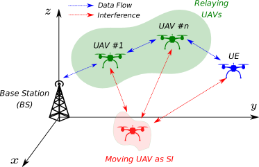
Figure 2: System model for the communications scenario where the interferer is a smart moving UAV.

The above optimization problem is over multiple UAVs. In the following, we address the problem from both the perspective of UAV network and smart jammers.

IV-A From UAV Network Perspective

In the UAV network, the UAVs try to evade the smart interferers’ interference. For the power allocation, since there are no constraints on the interference of the UAVs to smart jammers, the best strategy is to transmit with full power. In the 3D trajectory design, the UAVs deploy the Cheeger constant metric and move toward the spatial gradients of the algebraic connectivity so as to maximize the flow of the network as in (22).

IV-B From the Smart Interferers’ Perspective

Here, we consider the problem from the perspective of moving smart interferers which can be assumed as other UAVs aiming at decreasing the flow of the network. To do this, we assume that the smart UAVs transmit with their full power and move towards the opposite direction of spatial gradient of the algebraic connectivity of the UAV network weighted Laplacian matrix. Thus, the moving direction for the moving smart interferers can be given by:

$$\frac{\partial\lambda_{2}({\mathcal{L}_{\mathbf{W}}})}{\partial x^{J}_{m}} =-{\mathbf{x}^{f}}^{T}\frac{\partial({{\mathcal{L}_{\mathbf{W}}}})}{\partial x^{J}_{m}}{\mathbf{x}^{f}}=-\sum_{p=1}^{N}\sum_{q=1}^{N}\frac{v_{p}^{f}}{\sqrt{w_{p}}}\frac{v_{q}^{f}}{\sqrt{w_{q}}}\left[\frac{\partial\mathcal{L}}{\partial x_{m}^{J}}\right]_{p,q}$$ (41)

$$=-\sum_{\{p,q:p\sim q\}}\left[\frac{v_{p}^{f}}{\sqrt{w_{p}}}-\frac{v_{q}^{f}}{\sqrt{w_{q}}}\right]^{2}\frac{\partial a_{p,q}}{\partial x^{J}_{m}},~{}\forall~{}m\in\mathcal{M}.$$ (42)

By moving along the opposite direction of spatial gradient of the second smallest eigenvalue of the weighted Laplacian matrix of the UAV network, the moving smart interferers can decrease the maximum flow between the BS and the UE. The partial derivative with respect $x_{m}^{J},~{}\forall~{}m\in\mathcal{M}$ can be obtained similar to (23) as follows:

$$\frac{\partial\textrm{SIR}_{i,j}}{\partial x^{J}_{m}}= \frac{10^{-\eta_{l}/10}|g_{j,m}|^{2}\alpha_{l}d_{j,m}^{-\alpha_{l}-2}(x_{j}-x^{J}_{m})}{\Big{(}{\sum\limits_{m\in\mathcal{M}}{P}_{m}^{\textrm{J}}\,|h_{j,m}|^{2}+\chi\sum\limits_{k\in{\mathcal{Q}}_{i,j}}u(d_{j,k}/r_{\textrm{int}})}\Big{)}^{2}}P_{i}\,|h_{i,j}|^{2}.$$ (43)

For $y$-axis and $z$-axis, similar equations can be obtained. We consider a parameter $\tau$ so as to adjust the level of smartness of the smart UAV. That means the smart UAV interferer can move every $\tau$ iterations. Thus, by decreasing the value of $\tau$ the moving interferer will be smarter as it can chase the relay UAVs faster. It should be noted that we consider the static interferer as naive interferer in this scenario.

TABLE I: Simulation Parameters

Parameter	Value
Path-loss exponents $(\alpha_{1},\alpha_{2})$	$2.05,2.32$
Maximum transmit power of the UAVs $(\textrm{P}_{\textrm{max}})$	$20\,\text{dBm}$
Transmit power of the interferers $(\textrm{P}_{m}^{\textrm{J}}$, $\forall m\,{\in}\,\mathcal{M})$	$30\,\text{dBm}$
Bandwidth $(\textrm{B})$	$10\,\text{KHz}$
Interference threshold $(\textrm{I}^{\textrm{th}}_{m}$, $\forall m\,{\in}\,\mathcal{M})$	$[{-}50,{-}10]\,\text{dBm}$
Interference radius $(r_{\textrm{int}})$	$5\,\text{m}$
Carrier frequency $(f_{\rm c})$	$2~{}\text{GHz}$
Smoothed step-function parameters $(\zeta,\kappa,{\color[rgb]{0,0,0}y_{0}})$	$1,10,10^{-3}$
Safety precaution priority $(\chi)$	$1$

V Simulation Results

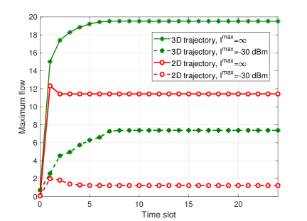
Figure 3: Convergence of the proposed alternating optimization problem.

In this section, we present numerical results based on extensive simulations, to evaluate the performance of the proposed joint 3D trajectory and power allocation optimization. In our simulation environment, the BS and the UE are assumed to be located at $(0,0,h^{\textrm{BS}})$ and $(200\,\text{m},0,h^{\textrm{UE}})$, respectively, in $\mathbb{R}^{3}$ with $h^{\textrm{BS}}\,{=}\,15\,\text{m}$. Moreover, the reckless interferers are located randomly in $xy-$plane with fixed altitude of $h^{\textrm{SI}}\,{=}\,20\,\text{m}$. The list of simulation parameters are given in Table I.

V-A Reckless Interferer

Here, we assume that the interferer acts as an reckless interferer which can be interpreted as a transceiver in the co-existing network.

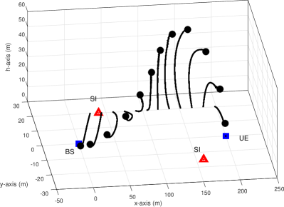
Figure 4: 3D trajectories of the UAVs in the presence of two reckless interferers (3D view).

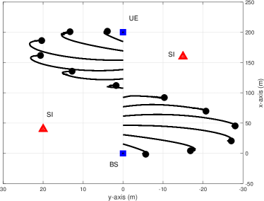
Figure 5: 3D trajectories of the UAVs in the presence of two reckless interferers (top view).

V-A1 Convergence of the Proposed Algorithm

In Fig. 3, the maximum flow of the network is depicted versus iterations. Each iteration is composed of solving one power allocation optimization problem and one trajectory design. We plotted the results for different value of $I^{\max}$, which determines the maximum value of tolerable interference form UAV network on the primary network. Apparently, the larger the $I^{\max}$, the larger data flow can be sent from the BS to UE as the UAVs can transmit with more power. We show the maximum flow of the network for 2D and 3D trajectory design approaches. For the $xy-$plane 2D trajectory design, we assume that each UAV can move in $xy-$plane and it can not move in $z$ direction (its height is assumed fixed). It can be seen that both algorithms converge in finite number of iterations, while the 3D trajectory design needs more time for convergence. However, 3D trajectory design significantly outperforms the 2D trajectory design and can double the transmission flow of the network. This performance improvement, which is one strong benefit of 3D trajectory design, is due to the fact that 3D space has more degrees of freedom as compared to 2D.

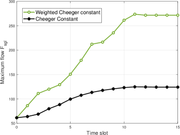
Figure 6: Maximum flow of the network for weighted and unweighted Cheeger constant.

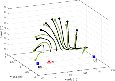
Figure 7: Different trajectories for weighted and unweighted Cheeger constant. Green and black trajectories are based on weighted and regular Cheeger constants, respectively.

In Fig. 4 and Fig. 5, the 3D trajectory of the UAVs are shown in 3D and top views, respectively, assuming 12 UAVs, 2 interferers, and a UE on the ground. We observe that the relaying UAVs adjust their locations in 3D space so as to evade from the interferers, and therefore improve the desired data flow between the BS and the UE.

V-A2 Impact of Weighted Cheeger Constant

We now look into the impact of using weighted version of Cheeger constant on the desired data flow and 3D trajectories. In Fig. 6, we depict the data flow for the conventional Cheeger constant and weighted Cheeger constant along with assuming 8 UAVs and a single SI. We observe that the weighted version is significantly superior to the conventional one with almost two times the desired data flow. We also exhibit the 3D UAV trajectories in Fig. 7. Interestingly, weighted Cheeger constant results in 3D trajectories ending up with final UAV locations closer to both the BS and UE. This may possibly be due to the fact that the bottleneck of the network flow occurs along with the closer links to both BS and UE considering the close proximity of the interferer located on the ground. The weighted Cheeger constant therefore adjusts the final UAV locations so as to make them as close to the BS and UE as possible.

V-A3 Interference Avoidance Capability

In Fig. 8, we depict the maximum flow against the interference threshold $\textrm{I}^{\textrm{th}}$ for the UE altitude of $h^{\textrm{UE}}\,{=}\,25\,\text{m}$, which may well represent a low-flying UAV as the desired UE. We consider 8 UAVs and one interferer on the ground. We observe that when the relaying UAVs are allowed to optimize their trajectories in 2D only (i.e., in $xy-$, $xz-$, or $yz-$ planes), their performances are always inferior to that of the 3D trajectory optimization. It can be seen that if the interferer transmit power is optimized, the UAV network performance can be further improved as the interferer will not produce stronger interference beyond satisfying the QoS constraint.

V-A4 Impact of the UE Altitude

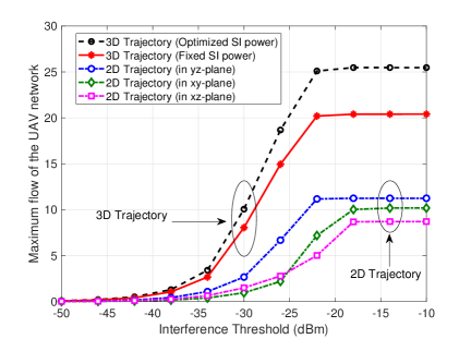
Figure 8: Maximum flow versus interference threshold for 2D and 3D trajectory optimization strategies along with optimal power allocation.

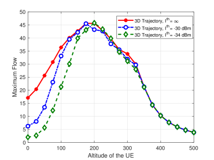
Figure 9: Maximum flow versus UE altitude for interference threshold of $\{{-}34,{-}30\}\,\text{dBm}$ as well as no interference (i.e., $\infty$) with 3D trajectories.

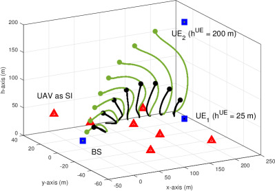
Figure 10: 3D trajectories for the results of Fig. 9 at UE altitudes of $\{25,200\}\,\text{m}$ (black trajectory is for 25 m and green trajectory is for 200 m.)

In Fig. 9, we present the maximum flow along with varying UE altitude of $h^{\textrm{UE}}\,{\in}\,[0,500]\,\text{m}$, which covers both on-ground and flying UEs. Interestingly, maximum flow improves with increasing altitude till $h^{\textrm{UE}}\,{=}\,200\,\text{m}$. To illustrate this situation, we depict the 3D trajectories of all the 8 UAVs in Fig. 10 for the UE altitudes of $h^{\textrm{UE}}\,{=}\,\{25,200\}\,\text{m}$. Moreover, the decrease in the maximum flow after $h^{\textrm{UE}}\,{=}\,200\,\text{m}$ is basically due to the increasing path loss, which now becomes more dominant over the interference (even though the interference is also decreasing due to the increasing distance).

V-B Smart Interferer

We finally consider a scenario involving two smart interferers, which are basically malicious UAVs, as discussed in Section IV-B. In order to evaluate its performance, we assume 12 UAVs and a UE at a height of 40 m (i.e., another UAV). The smart interferers starts its movement at $(100\,\text{m},0,20\,\text{m})$, and tries to impair the data flow of the UAV-assisted network as much as possible. This may equivalently be viewed as chasing the relaying UAVs. In Fig. 11 and Fig. 12, we depict the UAVs trajectories in 3D and 2D top view, respectively. We observe that while smart interferers are chasing the UAVs to decrease the data flow, the relaying UAVs adjust their locations to get away from the smart interferers.

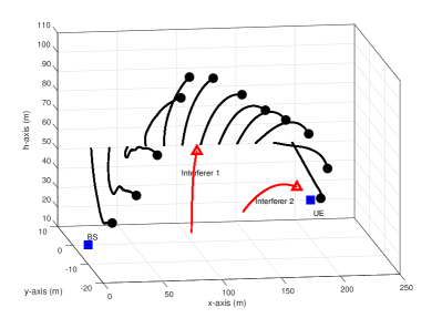
Figure 11: 3D trajectories of relaying UAVs, and the smart interferers acting as UAVs.

Note that we control the smartness of the interferer with the parameter $\tau$, which denotes the ability of the interferer to adjust its 3D location. The value of $\tau\,{=}\,1$ implies that the interferer can find its direction towards the “best” 3D location at the same speed of a relaying UAV. Considering a certain amount of time that the smart interferer needs to estimate the UAV-relaying parameters so as to decide the best strategy, we assume $\tau\,{>}\,1$ for more realistic situations. We assume $\tau\,{=}\,2$ for the 3D trajectories presented in Fig. 11 and Fig. 12. We also depict the data flow performance of the UAV-assisted network in Fig. 13 for smart interferers with $\tau\,{\in}\,\{1,2,6,10\}$ and the naive interferers which are not adjusting their locations. We observe that the data flow performance generally degrades as smart interferers become more capable in adjusting their locations (i.e., smaller $\tau$).

VI Conclusion

In this paper, we have considered the joint power and 3D trajectory design for a UAV-assisted relay network in the presence of an already existing network. A joint optimization solution for 3D trajectory design and power allocation is proposed based on spectral graph theory and convex optimization. Moreover, we considered the problem for both reckless and smart interferers. Simulation results show the effectiveness of the proposed algorithm in improving the maximum flow and interference mitigation. In particular, we have shown that the proposed 3D trajectory design can increase the UAV network maximum flow by more than two times while the interference threshold is satisfied on the primary existing network. Moreover, we have shown that there exists an optimal altitude for the UE as a UAV that maximizes the maximum flow of the UAV network. On the other hand, we observed that the UAVs can reconfigure their locations to evade the smart interferer, while smart interferers chase the UAVs so as to decrease the maximum flow of the network by increasing the interference resulted from decreasing the path loss effect.

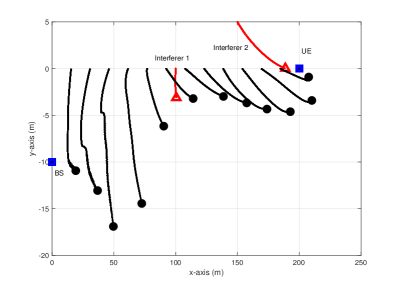
Figure 12: 3D trajectories for the UAVs trajectories moving while smart interferers as UAVs chasing them (top view).

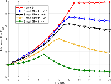
Figure 13: Maximum data flow of the UAV-assisted network with smart interferer, where decreasing $\tau$ corresponds to smarter interferer.

References

- [1] A. Rahmati, S. Hosseinalipour, Y. Yapici, X. He, I. Guvenc, H. Dai, and A. Bhuyan, “Interference avoidance in UAV-Assisted networks: Joint 3D trajectory design and power allocation,” in in Proc. IEEE Global Telecommun. Conf. (GLOBECOM), Big Island, HI, Dec. 2019, pp. 1–6.
- [2] S. Hayat, E. Yanmaz, and R. Muzaffar, “Survey on unmanned aerial vehicle networks for civil applications: A communications viewpoint,” IEEE Commun. Surveys Tuts., vol. 18, no. 4, pp. 2624–2661, 2016.
- [3] A. Rahmati, Y. Yapıcı, N. Rupasinghe, I. Guvenc, H. Dai, and A. Bhuyany, “Energy efficiency of RSMA and NOMA in cellular-connected mmWave UAV networks,” in Proc. IEEE ICC Workshops, Shanghai, China, May, 2019.
- [4] M. Erdelj, M. Król, and E. Natalizio, “Wireless sensor networks and multi-UAV systems for natural disaster management,” Computer Netw., vol. 124, pp. 72 – 86, 2017.
- [5] G. Ding, Q. Wu, L. Zhang, Y. Lin, T. A. Tsiftsis, and Y. Yao, “An amateur drone surveillance system based on the cognitive internet of things,” IEEE Commun. Mag., vol. 56, no. 1, pp. 29–35, Jan 2018.
- [6] B. Rabta, C. Wankmüller, and G. Reiner, “A drone fleet model for last-mile distribution in disaster relief operations,” Int. J. Disaster Risk Reduction, vol. 28, pp. 107–112, 2018.
- [7] N. Toorchi, F. Hu, E. Bentley, S. Pudlewski, and S. Kumar, “Volcano routing: a multi-pipe high-throughput routing protocol with hole avoidance for multi-beam directional mesh networks,” IEEE Transactions on Mobile Computing, pp. 1–1, 2019.
- [8] Y. Zeng, R. Zhang, and T. J. Lim, “Wireless communications with unmanned aerial vehicles: Opportunities and challenges,” IEEE Commun. Mag., vol. 54, no. 5, pp. 36–42, 2016.
- [9] A. Jaziri, R. Nasri, and T. Chahed, “Congestion mitigation in 5G networks using drone relays,” in Proc. IEEE Int. Wireless Commun. Mobile Comput. Conf. (IWCMC), Sep. 2016, pp. 233–238.
- [10] H. Baek and J. Lim, “Design of future UAV-relay tactical data link for reliable UAV control and situational awareness,” IEEE Commun. Mag., vol. 56, no. 10, pp. 144–150, 2018.
- [11] B. Li, Z. Fei, and Y. Zhang, “UAV communications for 5G and beyond: Recent advances and future trends,” IEEE Internet Things J., pp. 1–1, 2019.
- [12] M. Mozaffari, A. T. Z. Kasgari, W. Saad, M. Bennis, and M. Debbah, “Beyond 5G with UAVs: Foundations of a 3D wireless cellular network,” IEEE Trans. Wireless Commun., vol. 18, no. 1, pp. 357–372, 2019.
- [13] M. Mozaffari, W. Saad, M. Bennis, and M. Debbah, “Communications and control for wireless drone-based antenna array,” IEEE Trans. Commun., vol. 67, no. 1, pp. 820–834, Jan 2019.
- [14] A. Kumbhar, H. Binol, I. Guvenc, and K. Akkaya, “Interference coordination for aerial and terrestrial nodes in three-tier lte-advanced hetnet,” arXiv preprint arXiv:1809.00361, 2018.
- [15] Y. Zeng, J. Lyu, and R. Zhang, “Cellular-connected UAV: Potential, challenges, and promising technologies,” IEEE Wireless Commun., vol. 26, no. 1, pp. 120–127, February 2019.
- [16] S. Sekander, H. Tabassum, and E. Hossain, “Multi-tier drone architecture for 5G/B5G cellular networks: Challenges, trends, and prospects,” IEEE Commun. Mag., vol. 56, no. 3, pp. 96–103, March 2018.
- [17] M. Younis and K. Akkaya, “Strategies and techniques for node placement in wireless sensor networks: A survey,” Ad Hoc Networks, vol. 6, no. 4, pp. 621 – 655, 2008.
- [18] P. Zhan, K. Yu, and A. L. Swindlehurst, “Wireless relay communications using an unmanned aerial vehicle,” in Proc. IEEE 7th Workshop Signal Process. Advances Wireless Commun., Cannes, France, July, 2006.
- [19] Q. Wang, Z. Chen, W. Mei, and J. Fang, “Improving physical layer security using UAV-enabled mobile relaying,” IEEE Wireless Commun. Lett., vol. 6, no. 3, pp. 310–313, 2017.
- [20] U. Challita and W. Saad, “Network formation in the sky: Unmanned aerial vehicles for multi-hop wireless backhauling,” in Proc. IEEE Global Commun. Conf. (GLOBECOM), Singapore, Dec., 2017.
- [21] Y. Chen, N. Zhao, Z. Ding, and M. Alouini, “Multiple UAVs as relays: Multi-Hop single link versus multiple dual-hop links,” IEEE Trans. Wireless Commun., vol. 17, no. 9, pp. 6348–6359, Sep. 2018.
- [22] S. Hosseinalipour, A. Rahmati, and H. Dai, “Interference avoidance position planning in UAV-assisted wireless communication,” in Proc. IEEE Int. Conf. Commun. (ICC), Shanghai, China, May, 2019.
- [23] O. J. Faqir, Y. Nie, E. C. Kerrigan, and D. Gündüz, “Energy-efficient communication in mobile aerial relay-assisted networks using predictive control,” IFAC-PapersOnLine, vol. 51, no. 20, pp. 197–202, 2018.
- [24] Y. Chen, W. Feng, and G. Zheng, “Optimum placement of UAV as relays,” IEEE Commun. Lett., vol. 22, no. 2, pp. 248–251, Feb 2018.
- [25] S. Zhang, H. Zhang, Q. He, K. Bian, and L. Song, “Joint trajectory and power optimization for UAV relay networks,” IEEE Commun. Lett., vol. 22, no. 1, pp. 161–164, 2018.
- [26] Y. Zeng, R. Zhang, and T. J. Lim, “Throughput maximization for UAV-enabled mobile relaying systems,” IEEE Trans. Commun., vol. 64, no. 12, pp. 4983–4996, 2016.
- [27] F. Ono, H. Ochiai, and R. Miura, “A wireless relay network based on unmanned aircraft system with rate optimization,” IEEE Trans. Wireless Commun., vol. 15, no. 11, pp. 7699–7708, 2016.
- [28] J. Chen and D. Gesbert, “Local map-assisted positioning for flying wireless relays,” arXiv preprint arXiv:1801.03595, 2018.
- [29] M. M. U. Chowdhury, S. J. Maeng, E. Bulut, and I. Guvenc, “Effects of 3D antenna radiation and two-hop relaying on optimal UAV trajectory in cellular networks,” in Proc. IEEE Aerospace Conf., Big Sky, ID, Mar. 2019.
- [30] S. Hosseinalipour, A. Rahmati, and H. Dai, “Interference avoidance position planning in dual-hop and multi-hop UAV relay networks,” arXiv preprint arXiv:1907.01930, 2019.
- [31] S. Yin, J. Tan, and L. Li, “UAV-assisted cooperative communications with wireless information and power transfer,” arXiv preprint arXiv:1710.00174, 2017.
- [32] M. Tavana, A. Rahmati, V. Shah-Mansouri, and B. Maham, “Cooperative sensing with joint energy and correlation detection in cognitive radio networks,” IEEE Commun. Lett., vol. 21, no. 1, pp. 132–135, 2017.
- [33] N. Ahmed, S. S. Kanhere, and S. Jha, “On the importance of link characterization for aerial wireless sensor networks,” IEEE Commun. Mag., vol. 54, no. 5, pp. 52–57, 2016.
- [34] R. Weibel and R. J. Hansman, “Safety considerations for operation of different classes of UAVs in the NAS,” in AIAA 4th Aviation Technology, Integration and Operations (ATIO) Forum, 2004, p. 6244.
- [35] X. He, H. Dai, and P. Ning, “Dynamic adaptive anti-jamming via controlled mobility,” IEEE Trans. Wireless Commun., vol. 13, no. 8, pp. 4374–4388, Aug 2014.
- [36] A. Rahmati, X. He, I. Guvenc, and H. Dai, “Dynamic mobility-aware interference avoidance for aerial base stations in cognitive radio networks,” in Proc. IEEE INFOCOM, Paris, France, May 2019.
- [37] J. C. Bezdek and R. J. Hathaway, “Some notes on alternating optimization,” in AFSS Int. Conf. on Fuzzy Sys. Springer, 2002, pp. 288–300.
- [38] L. R. Ford Jr and D. R. Fulkerson, Flows in networks. Princeton University Press, 2015.
- [39] F. R. Chung and F. C. Graham, Spectral graph theory. American Mathematical Soc., 1997, no. 92.
- [40] M. Grant and S. Boyd, “CVX: Matlab software for disciplined convex programming, version 2.1,” 2014.
- [41] M. Chiang, C. W. Tan, D. P. Palomar, D. O’Neill, and D. Julian, “Power control by geometric programming,” Resource Allocation in Next Generation Wireless Networks, vol. 5, pp. 289–313, 2005.
- [42] S. Boyd and L. Vandenberghe, Convex optimization. Cambridge university press, 2004.
- [43] A. A. Nasir, D. T. Ngo, X. Zhou, R. A. Kennedy, and S. Durrani, “Joint resource optimization for multicell networks with wireless energy harvesting relays,” IEEE Trans. Vehi. Technol., vol. 65, no. 8, pp. 6168–6183, 2016.
- [44] B. Khamidehi, A. Rahmati, and M. Sabbaghian, “Joint sub-channel assignment and power allocation in heterogeneous networks: An efficient optimization method,” IEEE Commun. Lett., vol. 20, no. 12, pp. 2490–2493, 2016.