Device-independent certification of tensor products of quantum states using single-copy self-testing protocols

Ivan Šupić Affiliation: Département de Physique Appliquée, Université de Genève, 1211 Genève, Switzerland    Daniel Cavalcanti Affiliation: ICFO-Institut de Ciencies Fotoniques, The Barcelona Institute of Science and Technology, 08860 Castelldefels (Barcelona), Spain    Joseph Bowles Affiliation: ICFO-Institut de Ciencies Fotoniques, The Barcelona Institute of Science and Technology, 08860 Castelldefels (Barcelona), Spain
05.03.2021.
Abstract

Self-testing protocols are methods to determine the presence of shared entangled states in a device independent scenario, where no assumptions on the measurements involved in the protocol are made. A particular type of self-testing protocol, called parallel self-testing, can certify the presence of copies of a state, however such protocols typically suffer from the problem of requiring a number of measurements that increases with respect to the number of copies one aims to certify. Here we propose a procedure to transform single-copy self-testing protocols into a procedure that certifies the tensor product of an arbitrary number of (not necessarily equal) quantum states, without increasing the number of parties or measurement choices. Moreover, we prove that self-testing protocols that certify a state and rank-one measurements can always be parallelized to certify many copies of the state. Our results suggest a method to achieve device-independent unbounded randomness expansion with high-dimensional quantum states.

Introduction — Bell nonlocality describes measurement correlations which are rigidly incompatible with the notion of local determinism [Bel64, BCP+14]. Namely, all local deterministic theories satisfy bounds—called Bell inequalities—which limit the strength of the correlations between measurement outcomes of two spatially distant and non-communicating systems. Interestingly, it is possible to violate such Bell inequalities in quantum experiments [HBD+15, SMSC+15, GVW+15]. Such violating correlations, called nonlocal, are closely related to quantum resources such as entanglement and measurement incompatibility, essential for the development of modern day quantum technologies.

Bell nonlocality also plays a crucial role in so-called device-independent protocols. It turns out that the violation of a Bell inequality is a function of the observed correlations alone, regardless of the underlying physical realization. Thus, the sole observation of a Bell inequality violation witnesses the presence of both entanglement and incompatibility without having knowledge or making any assumptions about the underlying experimental implementation. Such an assumption-free verification is named device-independent and has a special significance in cryptographic scenarios [ABG+07, PAM+10].

The maximal violation of some Bell inequalities can even imply the precise form of the underlying state and measurements. This can be seen as a device-independent certification, and has received the name of self-testing [vB20, MY04]. The simplest example of such phenomenon is the maximal violation of the Clauser-Horn-Shimony-Holt (Bell) inequality [CHSH69], which can be used to self-test the maximally entangled pair of qubits and mutually unbiased local measurements [PR92, Tsi93, SW87].

There exist nonlocal correlations that self-test several copies of a quantum state, a process called parallel self-testing. These self-testing protocols have immediate applications in situations where high amounts of entanglement is needed, such as randomness expansion [CY14], parallel quantum key distribution [JMS20, Vid17], delegated quantum computing [RUV13, CGJV19], and universal entanglement certification [BŠCA18a]. One drawback of the first parallel self-testing protocols is that they require a number of local measurements that increases exponentially with the number of copies one wants to certify [WBMS16, Col17, CN16, McK17, BŠCA18b]. This fact increases the time-cost and the randomness consumption of the protocol (relevant for cryptographic applications). More recently, techniques to reduce the number of local measurements to poly(log(n)) and log(n) were found [NV17, NV18, CRSV18, OV16, BŠCA18b]. There exist protocols to self-test entangled states of arbitrary dimension with a constant number of three or four inputs per party [YN13, CGS17]. These protocols, when applied to copies of quantum states require making joint measurements between the local subsystems of each copy, making them challenging from an experimental perspective.

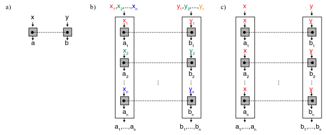
In this manuscript, we show a procedure to combine different self-testing protocols into a protocol that self tests tensor products of quantum states, without increasing the number of required measurements. The combined protocol has the advantage of not requiring joint measurements among the copies. As a key application, we show a way of self-testing nn copies of the two-qubit maximally entangled state using only two measurements per party (see Figure 1 c). This is the first self-testing protocol using the minimum number of local measurements possible for certifying an unbounded amount of entanglement. This procedure can therefore be used to convert one random bit into an arbitrary number of private random bits.

Figure 1: a) Standard Bell scenario, where local measurements labeled by xx and yy with outcomes aa and bb are performed on a shared state. b) Standard parallel self-testing protocol certifying nn copies of a quantum states. The measurement choice corresponds to a string of nn elements, each of them used to determine the measurement applied to each copy. Thus, the total number of local measurements increases exponentially with the number of copies one aims at certifying. c) The procedure we propose here (see Theorem 1) transforms a self-testing protocol for a single quantum state into a protocol for an arbitrary number of copies. Each party applies the same measurement to each copy and outputs each individual outcome.

Main idea of the method– For simplicity, we explain how our method can transform the self-testing based on the Clauser-Horn-Shimony-Holt (CHSH) game into a self-test for nn copies of a two-qubit maximally entangled state. The scenario consists of two space-like separated parties, Alice and Bob, making local measurements on a shared quantum system. Alice and Bob apply one of two measurements each, labeled x=0,1x=0,1 and y=0,1y=0,1 respectively, and their goal is to obtain outputs a=0,1a=0,1 and b=0,1b=0,1 such that ab=xya\oplus b=x\cdot y where \oplus is addition modulo 2. Their score is defined as ω=14x,yP(ab=xy|x,y)\omega=\frac{1}{4}\sum_{x,y}P(a\oplus b=x\cdot y|x,y), i.e. the probability of satisfying the winning condition averaged over a uniform choice of x,yx,y. Alice and Bob can use quantum resources to increase their score. In that case the inputs denote the measurement choices, while the outputs are simply measurement results. When they share quantum state ρAB\rho_{\mathrm{A}\mathrm{B}}, Alice performs measurements {𝖬a|x}a,x\{\mathsf{M}_{a|x}\}_{a,x}, and Bob {𝖭b|y}b,y\{\mathsf{N}_{b|y}\}_{b,y} the probabilities p(a,b|x,y)p(a,b|x,y) satisfy the Born rule p(a,b|x,y)=tr[𝖬a|x𝖭b|yρAB]p(a,b|x,y)=\operatorname{tr}\left[\mathsf{M}_{a|x}\otimes\mathsf{N}_{b|y}\rho_{\mathrm{A}\mathrm{B}}\right]. The measurement observables are defined as Ax=𝖬0|x𝖬1|x\mathrm{A}_{x}=\mathsf{M}_{0|x}-\mathsf{M}_{1|x} and By=𝖭0|y𝖭1|y\mathrm{B}_{y}=\mathsf{N}_{0|y}-\mathsf{N}_{1|y}. If Alice and Bob make use of classical resources (or separable states), the best score they can achieve is ω=34\omega=\frac{3}{4}, which is equivalent to satisfying the CHSH Bell inequality

A0B0+A0B1+A1B0A1B12,\displaystyle\langle\mathrm{A}_{0}\mathrm{B}_{0}\rangle+\langle\mathrm{A}_{0}\mathrm{B}_{1}\rangle+\langle\mathrm{A}_{1}\mathrm{B}_{0}\rangle-\langle\mathrm{A}_{1}\mathrm{B}_{1}\rangle\leq 2, (1)

where AxBy=ab(1)a+bP(a,b|x,y)\langle\mathrm{A}_{x}\mathrm{B}_{y}\rangle=\sum_{ab}(-1)^{a+b}P(a,b|x,y). On the other hand, if they share a maximally entangled pair of qubits |ϕ+=12[|00+|11]{\lvert\phi^{+}\rangle}=\frac{1}{\sqrt{2}}[{\lvert 00\rangle}+{\lvert 11\rangle}], Alice’s measurements correspond to the Pauli observables A0=σ𝖹\mathrm{A}_{0}=\sigma_{\mathsf{Z}} and A1=σ𝖷\mathrm{A}_{1}=\sigma_{\mathsf{X}} and Bob’s measurements to B0=(σ𝖹+σ𝖷)/2σ+\mathrm{B}_{0}=(\sigma_{\mathsf{Z}}+\sigma_{\mathsf{X}})/\sqrt{2}\equiv\sigma_{+} and B1=(σ𝖹σ𝖷)/2σ\mathrm{B}_{1}=(\sigma_{\mathsf{Z}}-\sigma_{\mathsf{X}})/\sqrt{2}\equiv\sigma_{-}, they can achieve the score ωq0.8536\omega_{q}\approx 0.8536. This strategy violates the CHSH Bell inequality to a value of 222\sqrt{2}, and is the largest violation possible in quantum theory. This maximum value is also known to self-test the state |ϕ+{\lvert\phi^{+}\rangle}. Thus, up to a possible local change of basis and extra unused degrees of freedom, the state |ϕ+{\lvert\phi^{+}\rangle} is the only state that achieves this value.

The CHSH inequality can also be used to self-test nn copies of |ϕ+n{\lvert\phi^{+}\rangle}^{\otimes n} via parallel self-testing [Col17, McK17]. For that purpose Alice and Bob in each round receive nn-bit inputs 𝐱=(x1,x2,,xn)\mathbf{x}=(x_{1},x_{2},\cdots,x_{n}) and 𝐲=(y1,y2,,yn)\mathbf{y}=(y_{1},y_{2},\cdots,y_{n}), and return nn-bit outputs 𝐚=(a1,a2,,an)\mathbf{a}=(a_{1},a_{2},\cdots,a_{n}) and 𝐛=(b1,b2,,bn)\mathbf{b}=(b_{1},b_{2},\cdots,b_{n}). To self-test the state, Alice measures σ𝖹\sigma_{\mathsf{Z}} or σ𝖷\sigma_{\mathsf{X}} on her local qubit ii depending on xi=0,1x_{i}=0,1, and Bob does similarly, measuring σ+\sigma_{+} or σ\sigma_{-} depending on yi=0,1y_{i}=0,1 and returning outcome bib_{i} (see Fig. 1b). The resulting correlations maximally violate nn CHSH inequalities in parallel and imply Alice and Bob share a tensor product of nn maximally entangled pairs of qubits.

We consider, in turn, a scenario in which each party has only two choices of measurements x=0,1x=0,1 and y=0,1y=0,1 (Fig. 1c). If x=0x=0 Alice measures all of her qubits in the σ𝖹\sigma_{\mathsf{Z}}-basis, whereas if x=1x=1 she measures all of them in the σ𝖷\sigma_{\mathsf{X}}-basis. In both cases she returns an output consisting of nn bits 𝐚=(a1,a2,,an)\mathbf{a}=(a_{1},a_{2},\cdots,a_{n}) corresponding to the outcomes of each of the nn measurements. Bob proceeds similarly, measuring all his qubits in σ+\sigma_{+} and σ\sigma_{-} bases and returning 𝐛=(b1,b2,,bn)\mathbf{b}=(b_{1},b_{2},\cdots,b_{n}). For any pair (ai,bi)(a_{i},b_{i}), the condition P(aibi=xy)=ωqP(a_{i}\oplus b_{i}=x\cdot y)=\omega_{q} is satisfied, and one might naively think that this information alone is enough to conclude that the state is |ϕ+n{\lvert\phi^{+}\rangle}^{\otimes n}. This would be a mistake however, as the following counter-example shows. Suppose Alice and Bob measure a single copy of |ϕ+{\lvert\phi^{+}\rangle}, obtaining outputs aa, bb such that P(ab=xy)=ωqP(a\oplus b=x\cdot y)=\omega_{q}. Then, they set ai=aa_{i}=a and bi=bb_{i}=b for all ii, leading to P(aibi=xy)=ωqP(a_{i}\oplus b_{i}=x\cdot y)=\omega_{q} for all ii. Thus, one can achieve P(aibi=xy)=ωqP(a_{i}\oplus b_{i}=x\cdot y)=\omega_{q} for all ii with only a single copy of |ϕ+{\lvert\phi^{+}\rangle}.

One thus needs to consider more information than just the CHSH score of each copy. One possibility is to consider the marginal statistics, since in the parallel nn-copy strategy one has p(𝐚|x)=1/2np(\mathbf{a}|x)=1/2^{n} whereas in the single-copy strategy the local output bits aia_{i} are always perfectly correlated (with a similar situation for Bob). However this will not work, since by using nn bits of pre-shared randomness (λ1,,λnCLOSE(\lambda_{1},\cdots,\lambda_{n}) and post-processing their outputs according to ai=a+λia_{i}=a+\lambda_{i} and bi=b+λib_{i}=b+\lambda_{i}, the local output bits of the single-copy strategy can be decorrelated without affecting the CHSH scores. Notice however, that there is still a crucial difference between the two strategies that remains: in each round of the single-copy strategy, if the first pair satisfies a1+b1=xya_{1}+b_{1}=x\cdot y, then all other pairs also satisfy ai+bi=xya_{i}+b_{i}=x\cdot y. This is not the case for the nn-copy strategy, where each pair has a probability ωq\omega_{q} to satisfy the condition in each round, independent of the other pairs. It is precisely this difference that we use as an inspiration to design our self-testing protocol.

The main result– Before stating our main result, let us define self-testing in a precise way. Consider a general bipartite Bell scenario, where x,y{0,1,,m1}x,y\in\{0,1,\cdots,m-1\} and a,b{0,1,,o1}{a},{b}\in\{0,1,\cdots,o-1\}. Alice and Bob share the state ρAB=trP[|ψψ|ABP]\rho_{\mathrm{A}\mathrm{B}}=\operatorname{tr}_{\mathrm{P}}\left[{\lvert\psi\rangle}{\langle\psi\rvert}_{\mathrm{A}\mathrm{B}\mathrm{P}}\right], with |ψABP{\lvert\psi\rangle}_{\mathrm{A}\mathrm{B}\mathrm{P}} being any purification of ρAB\rho_{\mathrm{A}\mathrm{B}}.

The probabilities of obtaining outputs aa and bb, when the inputs are xx and yy, respectively, are given by

p(a,b|x,y)=ψ|𝖬a|x𝖭b|y𝟙P|ψ,\displaystyle p(a,b|x,y)={\langle\psi\rvert}\mathsf{M}_{{a}|x}\otimes\mathsf{N}_{{b}|y}\otimes\mathbbm{1}_{\mathrm{P}}{\lvert\psi\rangle}, (2)

where {𝖬a|x}\{\mathsf{M}_{{a}|x}\} and {𝖭b|y}\{\mathsf{N}_{{b}|y}\} are Alice’s and Bob’s local measurement operators. We say that the probabilities {p(a,b|x,y)}\{p(a,b|x,y)\} self-test the reference experiment {|ψAB,𝖬a|x,𝖭b|y}\{{\lvert\psi^{\prime}\rangle}_{\mathrm{A}^{\prime}\mathrm{B}^{\prime}},\mathsf{M}^{\prime}_{{a}|x},\mathsf{N}^{\prime}_{{b}|y}\} if observing them in an experiment implies the existence of a local unitary transformation U=UAAVBB𝟙PU=U_{\mathrm{A}\mathrm{A}^{\prime}}\otimes V_{\mathrm{B}\mathrm{B}^{\prime}}\otimes\mathbbm{1}_{\mathrm{P}} such that

U[|ψABP|00AB]=|ξABP|ψAB;\displaystyle U\left[{\lvert\psi\rangle}_{\mathrm{A}\mathrm{B}\mathrm{P}}\otimes{\lvert 00\rangle}_{\mathrm{A}^{\prime}\mathrm{B}^{\prime}}\right]={\lvert\xi\rangle}_{\mathrm{A}\mathrm{B}\mathrm{P}}\otimes{\lvert\psi^{\prime}\rangle}_{\mathrm{A}^{\prime}\mathrm{B}^{\prime}};
U[𝖬a|x𝖭b|y𝟙P|ψABP|00AB]=\displaystyle U\left[{\mathsf{M}}_{{a}|x}\otimes{\mathsf{N}}_{{b}|y}\otimes\mathbbm{1}_{\mathrm{P}}{\lvert\psi\rangle}_{\mathrm{A}\mathrm{B}\mathrm{P}}\otimes{\lvert 00\rangle}_{\mathrm{A}^{\prime}\mathrm{B}^{\prime}}\right]= (3)
=|ξABP(𝖬a|x𝖭b|y|ψAB).\displaystyle\qquad\qquad\qquad={\lvert\xi\rangle}_{\mathrm{A}\mathrm{B}\mathrm{P}}\otimes\left({\mathsf{M}}^{\prime}_{{a}|x}\otimes{\mathsf{N}^{\prime}}_{{b}|y}{\lvert\psi^{\prime}\rangle}_{\mathrm{A}^{\prime}\mathrm{B}^{\prime}}\right).

These equations state that, up to ancillary degrees of freedom and local basis transformations, the state |ψ{\lvert\psi\rangle} is equivalent to |ψ{\lvert\psi^{\prime}\rangle}, and the measurements 𝖬a|x\mathsf{M}_{{a}|x} and 𝖭b|y\mathsf{N}_{{b}|y} act on |ψ{\lvert\psi\rangle} in the same way as 𝖬a|x\mathsf{M}^{\prime}_{{a}|x} and 𝖭b|y\mathsf{N}^{\prime}_{{b}|y} act on |ψ{\lvert\psi^{\prime}\rangle}. The state |ξ{\lvert\xi\rangle} is usually called the junk state and it can be seen as the state of additional degrees of freedom. Finally, let us define a Bell expression \mathcal{I}, as a linear combination of experimental probabilities =abxyba,bx,yp(a,b|x,y)\mathcal{I}=\sum_{abxy}b_{a,b}^{x,y}p(a,b|x,y), where ba,bx,yb_{a,b}^{x,y}\in\mathbb{R}.

Now we can state our main result:

Theorem 1.

Consider a Bell expression \mathcal{I} and {p(a,b|x,y)}\{p(a,b|x,y)\} for a scenario where Alice and Bob have mm inputs and oo outputs each, such that the value ({p(a,b|x,y)})=β\mathcal{I}(\{p(a,b|x,y)\})=\beta self-tests the reference experiment R={|ψ,𝖬a|x,𝖭b|y}R=\{{\lvert\psi^{\prime}\rangle},\mathsf{M}^{\prime}_{a|x},\mathsf{N}^{\prime}_{b|y}\}, where 𝖬a|x,𝖭b|y\mathsf{M}^{\prime}_{a|x},\mathsf{N}^{\prime}_{b|y} are rank-one projectors and p(a,b|x,y)>0a,bp(a,b|x,y)>0\penalty\ \forall\penalty\ a,b for each combination (x,y)(x,y) appearing in \mathcal{I}. Consider the scenario of Fig. 1b with mm inputs and ono^{n} outputs per party. Then, there exists a collection of nn non-linear Bell expressions 𝒥i\mathcal{J}^{i} (i=1,,ni=1,...,n) for this scenario that self-test the reference experiment Rn={|ψn,i=1n𝖬ai|x,i=1n𝖭bi|y}R_{n}=\{{\lvert\psi^{\prime}\rangle}^{\otimes n},\otimes_{i=1}^{n}\mathsf{M}^{\prime}_{a_{i}|x},\otimes_{i=1}^{n}\mathsf{N}^{\prime}_{b_{i}|y}\}.

The nonlinear Bell expressions 𝒥i\mathcal{J}^{i} in Theorem 1 are constructed as follows. Define 1=({p(a1,b1|x,y)})\mathcal{I}^{1}=\mathcal{I}(\{p(a_{1},b_{1}|x,y)\}) and the conditional Bell expressions for the pair i>1i>1 as

𝐚i1𝐛i1i=({p(ai,bi|x,y,𝐚i1,𝐛i1}),\displaystyle\mathcal{I}_{\mathbf{a}_{i-1}\mathbf{b}_{i-1}}^{i}=\mathcal{I}(\{p(a_{i},b_{i}|x,y,\mathbf{a}_{i-1},\mathbf{b}_{i-1}\}), (4)

where 𝐚i1=(a1,a2,,ai1)\mathbf{a}_{i-1}=(a_{1},a_{2},\cdots,a_{i-1}) and 𝐛i1=(b1,b2,,bi1)\mathbf{b}_{i-1}=(b_{1},b_{2},\cdots,b_{i-1}). 𝐚i1𝐛i1i\mathcal{I}_{\mathbf{a}_{i-1}\mathbf{b}_{i-1}}^{i} gives the value of \mathcal{I} for the pair ii conditioned on observing the particular values 𝐚i1=(a1,a2,,ai1)\mathbf{a}_{i-1}=(a_{1},a_{2},\cdots,a_{i-1}) and 𝐛i1=(b1,b2,,bi1)\mathbf{b}_{i-1}=(b_{1},b_{2},\cdots,b_{i-1}). Note that in order for these conditional Bell expressions to be well defined we require that p(𝐚i1,𝐛i1|x,y)>0𝐚i1,𝐛i1p(\mathbf{a}_{i-1},\mathbf{b}_{i-1}|x,y)>0\penalty\ \forall\penalty\ \mathbf{a}_{i-1},\mathbf{b}_{i-1} for each combination (x,y)(x,y) appearing in \mathcal{I}. This is automatically the case for the reference experiment RnR_{n} due to the properties of RR given in the statement of the theorem. The Bell expression 𝒥i\mathcal{J}^{i} is defined as

𝒥i=1o2(i1)𝐚i1𝐛i1𝐚i1𝐛i1i,\displaystyle\mathcal{J}^{i}=\frac{1}{o^{2(i-1)}}\sum_{\mathbf{a}_{i-1}\mathbf{b}_{i-1}}\mathcal{I}_{\mathbf{a}_{i-1}\mathbf{b}_{i-1}}^{i}, (5)

for i>1i>1 and 𝒥1=1\mathcal{J}^{1}=\mathcal{I}^{1}. The observation that 𝒥i=βi=1,,n\mathcal{J}^{i}=\beta\penalty\ \forall i=1,\cdots,n self tests RnR_{n}. The proof is inductive (given a self-test of kk copies, the value of 𝒥k+1\mathcal{J}^{k+1} self-tests an additional copy) and is given in the Appendix A. Here we provide some intuition behind the proof. As shown on the example of the CHSH inequality two ingredients are necessary to make a self-testing statement with the minimal number of inputs. First, all sets of probabilities p(ai,bi|x,y)p(a_{i},b_{i}|x,y) reach the maximum of \mathcal{I}, and the pairs of outputs (ai,bi)(a_{i},b_{i}) are mutually independent. If 𝒥i\mathcal{J}^{i} takes value β\beta for all ii, it means that all conditional Bell expressions 𝐚i1𝐛i1i\mathcal{I}_{\mathbf{a}_{i-1}\mathbf{b}_{i-1}}^{i} are also equal to β\beta. It can be shown that the maximal values of conditional Bell expressions imply that the outputs corresponding to different ii-s are mutually independent. In other words, conditioning on 𝐚i1,𝐛i1\mathbf{a}_{i-1},\mathbf{b}_{i-1} does not affect the values of aia_{i} and bib_{i}. Hence, β=(p(ai,bi|x,y,𝐚i1,𝐛i1)=(p(ai,bi|x,y)\beta=\mathcal{I}(p(a_{i},b_{i}|x,y,\mathbf{a}_{i-1},\mathbf{b}_{i-1})=\mathcal{I}(p(a_{i},b_{i}|x,y), for all ii-s, which means that both conditions for making a self-testing statement are met.

A direct consequence of Theorem 1 is the possibility of self-testing nn copies of the two-qubit maximally entangled state |ϕ+{\lvert\phi^{+}\rangle} (itself a maximally entangled state of local dimension 2n2^{n}) with only two measurement settings per party via the CHSH Bell inequality. More precisely, we have the following corollary:

Corollary 1.

Let 𝖬a|x,𝖭b|y\mathsf{M}_{a|x},\mathsf{N}_{b|y} (x,y{0,1},a,b{±1}x,y\in\{0,1\},a,b\in\{\pm 1\}) be the local measurements that lead to the maximal violation of the CHSH Bell inequality when applied to |ϕ+{\lvert\phi^{+}\rangle}. Then the correlations obtained by performing the experiment R={|ϕ+,𝖬a|x,𝖭b|y}R=\{{\lvert\phi^{+}\rangle},\mathsf{M}_{a|x},\mathsf{N}_{b|y}\} in the parallel scheme of Fig. 1c self-test the reference experiment {|ϕ+n,𝖬a|xn,𝖭b|yn}\{{\lvert\phi^{+}\rangle}^{\otimes n},\mathsf{M}_{a|x}^{\otimes n},\mathsf{N}_{b|y}^{\otimes n}\}

In particular, this means that an unbounded amount of entanglement can be certified in a device-independent manner with the minimum number of local measurements possible.

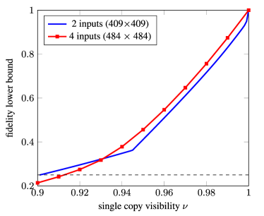
Although Theorem 1 holds only for the case of perfect statistics, one can investigate the robustness to noise of Corollary 1 for the case n=2n=2, via the technique propsed in [BNS+15, YVB+14]. The precise noise model we consider is one in which each copy of the state is subject to the same level of white noise. That is, the observed correlations are generated using the same measurement strategy on the state ρνρν\rho_{\nu}\otimes\rho_{\nu} where

ρν=ν|ϕ+ϕ+|+(1ν)𝟙/4.\displaystyle\rho_{\nu}=\nu{\lvert\phi^{+}\rangle\!\langle\phi^{+}\rvert}+(1-\nu)\mathbbm{1}/4. (6)

In [BNS+15, YVB+14] a semi-definite program is given that calculates a value ff, such that for any state ρAB\rho_{\mathrm{A}\mathrm{B}} leading to the observed correlations, there exists a local transformation mapping ρAB\rho_{\mathrm{A}\mathrm{B}} to a state that has fidelity at least ff with the reference state (in this case |ϕ+|ϕ+){\lvert\phi^{+}\rangle}\otimes{\lvert\phi^{+}\rangle}). In the case of perfect self-testing (Device-independent certification of tensor products of quantum states using single-copy self-testing protocols), one has f=1f=1, which then decreases as a function of the noise parameter. Fig. 2 shows the values of ff obtained as a function of ν\nu for this noise model.

Figure 2: Lower bounds to the self-tested fidelity with the state |ϕ+|ϕ+{\lvert\phi^{+}\rangle}\otimes{\lvert\phi^{+}\rangle} obtained via the method proposed in Refs. [BNS+15, YVB+14], using correlations obtained from two copies of the isotropic state ν|ϕ+ϕ+|+(1ν)𝟙/4\nu{\lvert\phi^{+}\rangle\!\langle\phi^{+}\rvert}+(1-\nu)\mathbbm{1}/4. The blue curve is obtained using two inputs per party, using the parallel scheme of Fig. 1c. The red curve is data taken from [WBMS16] using the strategy of Fig. 1b with four inputs per party. The legend gives the size of the matrices used in the corresponding SDP optimization. The dashed line corresponds to the trivial fidelity between the target state and the separable state |00{\lvert 00\rangle} of 0.25.

Extensions – Theorem 1 is defined for bipartite Bell inequalities that feature an equal number of inputs per party. Here we present some more general extensions to this result that either do not require the knowledge of a specific Bell inequality, or allow one to self-test tensor products of different bipartite states.

Parallel self-testing protocols from full statistics—While Theorem 1 refers to self-tests based on the maximal violation of some Bell inequality, it is worth noting that similar claims can be made for self-testing protocols based on the observation of a particular set of correlations. More precisely, we have the following result.

Theorem 2.

Assume that the correlations {p(a,b|x,y)}\{p(a,b|x,y)\} self-test the reference state |ψ{\lvert\psi^{\prime}\rangle}, such that p(a,b|x,y)>0p(a,b|x,y)>0 for all a,b,x,ya,b,x,y. Then the correlations {p(𝐚,𝐛|x,y)}\{p(\mathbf{a},\mathbf{b}|x,y)\} obtained by performing the reference experiment nn times in the parallel scheme of Fig. 1c self-test the corresponding tensor product |ψn{\lvert\psi^{\prime}\rangle}^{\otimes n}.

In Appendix B we give an example of this technique that self-tests tensor products of the maximally entangled two-qubit state based on the correlations presented in [WWS16].

Combining self-testing protocols—The previous results show how it is possible to self-test a tensor product |ψn{\lvert\psi^{\prime}\rangle}^{\otimes n} of the same state |ψ{\lvert\psi^{\prime}\rangle}, starting from a given protocol to self-test the state |ψ{\lvert\psi^{\prime}\rangle}. In fact, the following describes how our construction can also be used to generate self-testing protocols for a tensor product of different states i|ψi\bigotimes_{i}{\lvert\psi_{i}^{\prime}\rangle}.

Theorem 3.

Consider a set of states {|ψi}\{{\lvert\psi_{i}^{\prime}\rangle}\}, each of which is self-tested through the maximal value of a corresponding Bell expression i\mathcal{I}_{i}, where each i\mathcal{I}_{i} features the same number of inputs for each party. Then the correlations {p(𝐚,𝐛|x,y)}\{p(\mathbf{a},\mathbf{b}|x,y)\} obtained by performing the reference experiments nn times in the parallel scheme of Fig. 1c self-test the state i|ψi\bigotimes_{i}{\lvert\psi_{i}^{\prime}\rangle}.

The proof of this is almost identical to the proof of Theorem 1, instead now in (4) the Bell expressions i\mathcal{I}_{i} are different for each ii; see Appendix C for more details. One implication of this is the possibility to self-test a tensor product of different partially entangled pairs of qubits with two inputs for each party, which can be achieved through the use of different tilted CHSH inequalities [BP15].

All self-testing protocols can be paralellized— Here we discuss conditions for parallel self-testing without aiming to keep the number of inputs constant. As mentioned in the introduction, a number of schemes to parallel self-test certain classes of states are known (see [Col17, McK17, CN16, KM18, BKM19]), where the number of inputs scales exponentially with the number of copies to be self-tested. Given these examples, one interesting question is thus whether any self-testing protocol for a state |ψ{\lvert\psi\rangle} can be ‘parallelized’ to self-test the tensor product |ψn{\lvert\psi\rangle}^{\otimes n}, at the expense of having exponentially many inputs. We give a positive answer to this question, answering an even a more general question of self-testing a tensor product i|ψi\bigotimes_{i}{\lvert\psi_{i}\rangle} of different states, given that there are self-tests for the individual states |ψi{\lvert\psi_{i}\rangle}. Note that unlike the previous results, no restrictions are needed on the reference correlations (i.e. some probabilities can be zero).

Theorem 4.

Consider a set of nn bipartite Bell expressions {i}\{\mathcal{I}_{i}\} characterised by mim_{i} inputs and oio_{i} outputs, respectively, such that the value i({p(ai,bi|xi,yi)})=βi\mathcal{I}_{i}(\{p(a_{i},b_{i}|x_{i},y_{i})\})=\beta_{i} self-tests the reference experiment Ri={|ψi,𝖬ai|xi,𝖭bi|yi}R_{i}=\{{\lvert\psi_{i}^{\prime}\rangle},\mathsf{M}^{\prime}_{a_{i}|x_{i}},\mathsf{N}^{\prime}_{b_{i}|y_{i}}\}, where 𝖬ai|xi,𝖭bi|yi\mathsf{M}^{\prime}_{a_{i}|x_{i}},\mathsf{N}^{\prime}_{b_{i}|y_{i}} are rank-one projectors for each ii. Then, the correlations obtained by performing the RiR_{i}’s in parallel as in Fig. 1b self-test the reference experiment Rn={i=1|ψi,i𝖬ai|x,i=1n𝖭bi|y}R_{n}=\{\bigotimes_{i=1}{\lvert\psi_{i}^{\prime}\rangle},\bigotimes_{i}\mathsf{M}^{\prime}_{a_{i}|x},\otimes_{i=1}^{n}\mathsf{N}^{\prime}_{b_{i}|y}\}.

The result is proven by constructing a single Bell expression whose maximal value self-tests RnR_{n}. For each pair ii define the Bell value conditioned on particular choice of other inputs xj,yjx_{j},y_{j}, jij\neq i:

𝐱(i)𝐲(i)i=𝐚(i),𝐛(i)i(p(𝐚,𝐛|𝐱,𝐲))\mathcal{I}^{i}_{\mathbf{x}_{(i)}\mathbf{y}_{(i)}}=\sum_{\mathbf{a}_{(i)},\mathbf{b}_{(i)}}\mathcal{I}_{i}(p(\mathbf{a},\mathbf{b}|\mathbf{x},\mathbf{y})) (7)

where 𝐚(i)={a1,ai1,ai+1,,an}\mathbf{a}_{(i)}=\{a_{1},\cdots a_{i-1},a_{i+1},\cdots,a_{n}\} and similarly for 𝐛(i)\mathbf{b}_{(i)}, 𝐱(i)\mathbf{x}_{(i)} and 𝐲(i)\mathbf{y}_{(i)}. The Bell expression i\mathcal{I}_{i} averaged over all other inputs 𝐱(i)\mathbf{x}_{(i)} and 𝐲(i)\mathbf{y}_{(i)} is

𝒥i=1jimj2𝐱(i)𝐲(i)𝐱(i)𝐲(i)i.\mathcal{J}^{i}=\frac{1}{\prod_{j\neq i}m_{j}^{2}}\sum_{\mathbf{x}_{(i)}\mathbf{y}_{(i)}}\mathcal{I}^{i}_{\mathbf{x}_{(i)}\mathbf{y}_{(i)}}. (8)

If 𝒥i\mathcal{J}^{i} achieves its maximal value, it means that for for every 𝐱i\mathbf{x}_{i} and 𝐲i\mathbf{y}_{i} 𝐱i𝐲ii\mathcal{I}^{i}_{\mathbf{x}_{i}\mathbf{y}_{i}} also achieves the maximal value, which is enough to prove self-testing of the reference experiment RnR_{n}. The proof of the theorem is given in Appendix D.

Application: unbounded randomness expansion.– Self-testing is intrinsically related to device-independent randomness expansion [CY14, CK11, LLR+21]. This is because, once we certify that the system is in the state |ψ{\lvert\psi\rangle}, we can also conclude that any external system is uncorrelated to it. Thus, an external observer can not predict the outcomes of the measurements applied to the system of interest, i.e. the outcomes are random. In particular, if the state is maximally entangled of local dimension dd, and the measurements applied to it are rank-one projective, the amount of random bits obtained per round is log2(d)\log_{2}(d). Notice, however, that in a Bell test some initial amount of randomness must be consumed in the choice of inputs. Thus, the efficiency of the randomness generation protocol is typically given by the the trade-off between the initial randomness consumed and the final randomness obtained. Our Theorem 1 applied to the CHSH inequality and self-testing nn copies of a maximally entangled state shows that the best trade-off can be achieved from the noiseless correlations, where only one bit of randomness is used to generate log2(d)\log_{2}(d) bits or randomness per round. We thus suspect that our results could improve extraction rates of practical device-independent randomness expansion protocols, although this would require a closer look at issues of noise robustness.

Discussion–In this manuscript we introduced a new procedure useful in parallel self-testing. It allows to self-test highly entangled quantum states with a constant number of measurements. Such schemes are important in protocols for randomness expansion: a small amount of randomness can be expanded to a string of unbounded length. At the heart of our construction lies an interesting insight: independent Bell violations can be used to ensure independence of sources even when the measurements are perfectly correlated. There are several directions for future research on the topic. It would be interesting to explore noise robustness of our scheme. Furthermore, the condition for self-testing can be seen as the maximal violation of a non-linear Bell inequality. One might try to understand if this can be achieved using a single linear Bell inequality.

Note– While working on this project we became aware of the work [SSKA19] exploring self-testing of quantum systems of arbitrary local dimension with minimal number of measurements.

Acknowledgements— We thank Jean-Daniel Bancal for sharing numerical data, to Jed Kaniewski and Yeong-Cherng Liang for useful comments and suggestions and to the anonymous referee for many useful comments. We acknowledge funding from SNSF (grant DIAQ), Ramon y Cajal fellowship, the Government of Spain (FIS2020-TRANQI, Retos Quspin and Severo Ochoa CEX2019-000910-S), Fundació Cellex, Fundació Mir-Puig, Generalitat de Catalunya (CERCA, AGAUR SGR 1381),ERC AdG CERQUTE and the AXA Chair in Quantum Information Science.

References

  • [ABG+07] Antonio Acín, Nicolas Brunner, Nicolas Gisin, Serge Massar, Stefano Pironio, and Valerio Scarani. Device-independent security of quantum cryptography against collective attacks. Physical Review Letters, 98(23):230501, 2007. doi:10.1103/PhysRevLett.98.230501.
  • [BCP+14] Nicolas Brunner, Daniel Cavalcanti, Stefano Pironio, Valerio Scarani, and Stephanie Wehner. Bell nonlocality. Rev. Mod. Phys., 86:419–478, Apr 2014. doi:10.1103/RevModPhys.86.419.
  • [Bel64] John Stewart Bell. On the Einstein-Podolsky-Rosen paradox. Physics, 1:195–200, 1964. URL: https://cds.cern.ch/record/111654.
  • [BKM19] Spencer Breiner, Amir Kalev, and Carl A. Miller. Parallel self-testing of the GHZ state with a proof by diagrams. In Peter Selinger and Giulio Chiribella, editors, Proceedings of the 15th International Conference on Quantum Physics and Logic, Halifax, Canada, 3-7th June 2018, volume 287 of Electronic Proceedings in Theoretical Computer Science, pages 43–66. Open Publishing Association, 2019. doi:10.4204/EPTCS.287.3.
  • [BNS+15] Jean-Daniel Bancal, Miguel Navascués, Valerio Scarani, Tamás Vértesi, and Tzyh Haur Yang. Physical characterization of quantum devices from nonlocal correlations. Phys. Rev. A, 91:022115, Feb 2015. doi:10.1103/PhysRevA.91.022115.
  • [BP15] Cédric Bamps and Stefano Pironio. Sum-of-squares decompositions for a family of Clauser-Horne-Shimony-Holt-like inequalities and their application to self-testing. Phys. Rev. A, 91:052111, May 2015. doi:10.1103/PhysRevA.91.052111.
  • [BŠCA18a] Joseph Bowles, Ivan Šupić, Daniel Cavalcanti, and Antonio Acín. Device-independent entanglement certification of all entangled states. Phys. Rev. Lett., 121:180503, Oct 2018. doi:10.1103/PhysRevLett.121.180503.
  • [BŠCA18b] Joseph Bowles, Ivan Šupić, Daniel Cavalcanti, and Antonio Acín. Self-testing of Pauli observables for device-independent entanglement certification. Phys. Rev. A, 98:042336, Oct 2018. doi:10.1103/PhysRevA.98.042336.
  • [CGJV19] Andrea Coladangelo, Alex B Grilo, Stacey Jeffery, and Thomas Vidick. Verifier-on-a-leash: new schemes for verifiable delegated quantum computation, with quasilinear resources. In Annual International Conference on the Theory and Applications of Cryptographic Techniques, pages 247–277. Springer, 2019. doi:10.1007/978-3-030-17659-4_9.
  • [CGS17] Andrea Coladangelo, Koon Tong Goh, and Valerio Scarani. All pure bipartite entangled states can be self-tested. Nature Communications, 8:15485, may 2017. doi:10.1038/ncomms15485.
  • [CHSH69] John F. Clauser, Michael A. Horne, Abner Shimony, and Richard A. Holt. Proposed experiment to test local hidden-variable theories. Phys. Rev. Lett., 23:880–884, Oct 1969. doi:10.1103/PhysRevLett.23.880.
  • [CK11] Roger Colbeck and Adrian Kent. Private randomness expansion with untrusted devices. Journal of Physics A: Mathematical and Theoretical, 44(9):095305, 2011. doi:10.1088/1751-8113/44/9/095305.
  • [CN16] Matthew Coudron and Anand Natarajan. The parallel-repeated magic square game is rigid, 2016. arXiv:1609.06306. URL: https://arxiv.org/abs/1609.06306.
  • [Col17] Andrea Coladangelo. Parallel self-testing of (tilted) EPR pairs via copies of (tilted) CHSH and the magic square game. Quantum Information and Computation, 17(9-10):831–865, 2017. doi:10.26421/QIC17.9-10-6.
  • [CRSV18] Rui Chao, Ben W. Reichardt, Chris Sutherland, and Thomas Vidick. Test for a large amount of entanglement, using few measurements. Quantum, 2:92, September 2018. doi:10.22331/q-2018-09-03-92.
  • [CY14] Matthew Coudron and Henry Yuen. Infinite randomness expansion with a constant number of devices. In Proceedings of the Forty-sixth Annual ACM Symposium on Theory of Computing, STOC ’14, pages 427–436, New York, NY, USA, 2014. ACM. doi:10.1145/2591796.2591873.
  • [GVW+15] Marissa Giustina, Marijn A. M. Versteegh, Sören Wengerowsky, Johannes Handsteiner, Armin Hochrainer, Kevin Phelan, Fabian Steinlechner, Johannes Kofler, Jan-Åke Larsson, Carlos Abellán, Waldimar Amaya, Valerio Pruneri, Morgan W. Mitchell, Jörn Beyer, Thomas Gerrits, Adriana E. Lita, Lynden K. Shalm, Sae Woo Nam, Thomas Scheidl, Rupert Ursin, Bernhard Wittmann, and Anton Zeilinger. Significant-loophole-free test of bell’s theorem with entangled photons. Phys. Rev. Lett., 115:250401, Dec 2015. doi:10.1103/PhysRevLett.115.250401.
  • [HBD+15] B. Hensen, H. Bernien, A. E. Dréau, A. Reiserer, N. Kalb, M. S. Blok, J. Ruitenberg, R. F. L. Vermeulen, R. N. Schouten, C. Abellán, and et al. Loophole-free bell inequality violation using electron spins separated by 1.3 kilometres. Nature, 526(7575):682–686, 2015. doi:10.1038/nature15759.
  • [JMS20] Rahul Jain, Carl A. Miller, and Yaoyun Shi. Parallel device-independent quantum key distribution. IEEE Transactions on Information Theory, 66(9):5567–5584, Sep 2020. doi:10.1109/tit.2020.2986740.
  • [KM18] Amir Kalev and Carl A Miller. Rigidity of the magic pentagram game. Quantum Science and Technology, 3(1):015002, 2018. doi:10.1088/1367-2630/18/2/025021.
  • [LLR+21] Wen-Zhao Liu, Ming-Han Li, Sammy Ragy, Si-Ran Zhao, Bing Bai, Yang Liu, Peter J Brown, Jun Zhang, Roger Colbeck, Jingyun Fan, et al. Device-independent randomness expansion against quantum side information. Nature Physics, pages 1–4, 2021. doi:10.1038/s41567-020-01147-2.
  • [McK17] Matthew McKague. Self-testing in parallel with CHSH. Quantum, 1:1, April 2017. doi:10.22331/q-2017-04-25-1.
  • [MY04] Dominic Mayers and Andrew Yao. Self testing quantum apparatus. Quantum Info. Comput., 4:273, 2004. doi:10.26421/QIC4.4-3.
  • [NPA07] Miguel Navascués, Stefano Pironio, and Antonio Acín. Bounding the set of quantum correlations. Phys. Rev. Lett., 98:010401, Jan 2007. doi:10.1103/PhysRevLett.98.010401.
  • [NPA08] Miguel Navascués, Stefano Pironio, and Antonio Acín. A convergent hierarchy of semidefinite programs characterizing the set of quantum correlations. New Journal of Physics, 10(7):073013, 2008. doi:10.1088/1367-2630/10/7/073013.
  • [NV17] Anand Natarajan and Thomas Vidick. A quantum linearity test for robustly verifying entanglement. In Proceedings of the 49th Annual ACM SIGACT Symposium on Theory of Computing, STOC 2017, pages 1003–1015, New York, NY, USA, 2017. ACM. doi:10.1145/3055399.3055468.
  • [NV18] Anand Natarajan and Thomas Vidick. Low-degree testing for quantum states, and a quantum entangled games pcp for qma. In 2018 IEEE 59th Annual Symposium on Foundations of Computer Science (FOCS), pages 731–742, Oct 2018. doi:10.1109/FOCS.2018.00075.
  • [OV16] Dimiter Ostrev and Thomas Vidick. The structure of nearly-optimal quantum strategies for the CHSH (n) XOR games. Quantum Information & Computation, 16(13-14), pp.(13-14):1191–1211, 2016. doi:10.26421/QIC16.13-14-6.
  • [PAM+10] Stefano Pironio, Antonio Acín, Serge Massar, A Boyer de La Giroday, Dzimitry N Matsukevich, Peter Maunz, Steven Olmschenk, David Hayes, Le Luo, T Andrew Manning, et al. Random numbers certified by Bell’s theorem. Nature, 464(7291):1021–1024, 2010. doi:10.1038/nature09008.
  • [PR92] Sandu Popescu and Daniel Rohrlich. Which states violate Bell’s inequality maximally? Physics Letters A, 169(6):411–414, 1992. doi:10.1016/0375-9601(92)90819-8.
  • [RUV13] Ben W. Reichardt, Falk Unger, and Umesh Vazirani. Classical command of quantum systems. Nature, 496:456, 2013. doi:10.1038/nature12035.
  • [SMSC+15] Lynden K. Shalm, Evan Meyer-Scott, Bradley G. Christensen, Peter Bierhorst, Michael A. Wayne, Martin J. Stevens, Thomas Gerrits, Scott Glancy, Deny R. Hamel, Michael S. Allman, Kevin J. Coakley, Shellee D. Dyer, Carson Hodge, Adriana E. Lita, Varun B. Verma, Camilla Lambrocco, Edward Tortorici, Alan L. Migdall, Yanbao Zhang, Daniel R. Kumor, William H. Farr, Francesco Marsili, Matthew D. Shaw, Jeffrey A. Stern, Carlos Abellán, Waldimar Amaya, Valerio Pruneri, Thomas Jennewein, Morgan W. Mitchell, Paul G. Kwiat, Joshua C. Bienfang, Richard P. Mirin, Emanuel Knill, and Sae Woo Nam. Strong loophole-free test of local realism. Phys. Rev. Lett., 115:250402, Dec 2015. doi:10.1103/PhysRevLett.115.250402.
  • [SSKA19] Shubhayan Sarkar, Debashis Saha, Jedrzej Kaniewski, and Remigiusz Augusiak. Self-testing quantum systems of arbitrary local dimension with the minimal number of measurements, 2019. arXiv:1909.12722.
  • [SW87] Stephen J. Summers and Reinhard F. Werner. Maximal violation of Bell’s inequalities is generic in quantum field theory. Communications in Mathematical Physics, 110(2):247–259, 1987. doi:10.1007/BF01207366.
  • [Tsi93] Boris Tsirelson. Some results and problems on quantum Bell-type inequalities. Hadronis Journal Supplement, 8:329–45, 1993. URL: https://ci.nii.ac.jp/naid/10026857475/en/.
  • [vB20] Ivan Šupić and Joseph Bowles. Self-testing of quantum systems: a review. Quantum, 4:337, Sep 2020. doi:10.22331/q-2020-09-30-337.
  • [Vid17] Thomas Vidick. Parallel DIQKD from parallel repetition, 2017. arXiv:1703.08508.
  • [WBMS16] Xingyao Wu, Jean-Daniel Bancal, Matthew McKague, and Valerio Scarani. Device-independent parallel self-testing of two singlets. Phys. Rev. A, 93:062121, 2016. doi:10.1103/PhysRevA.93.062121.
  • [WWS16] Yukun Wang, Xingyao Wu, and Valerio Scarani. All the self-testings of the singlet for two binary measurements. New Journal of Physics, 18(2):025021, 2016. doi:10.1088/1367-2630/18/2/025021.
  • [YN13] Tzyh Haur Yang and Miguel Navascués. Robust self-testing of unknown quantum systems into any entangled two-qubit states. Phys. Rev. A, 87:050102, May 2013. doi:10.1103/PhysRevA.87.050102.
  • [YVB+14] Tzyh Haur Yang, Tamás Vértesi, Jean-Daniel Bancal, Valerio Scarani, and Miguel Navascués. Robust and versatile black-box certification of quantum devices. Phys. Rev. Lett., 113:040401, Jul 2014. doi:10.1103/PhysRevLett.113.040401.

v

Appendix A Proof of Theorem 1

Before starting the proofs let us introduce some useful notation. The probabilities to observe outcomes 𝐚=(a1,,an)\mathbf{a}=(a_{1},\cdots,a_{n}) and 𝐛=(b1,,bn)\mathbf{b}=(b_{1},\cdots,b_{n}) when the inputs are xx and yy are given by the Born rule:

p(𝐚,𝐛|x,y)=tr[𝖬𝐚|x𝖭𝐛|yρAB].p(\mathbf{a},\mathbf{b}|x,y)=\operatorname{tr}[\mathsf{M}_{\mathbf{a}|x}\otimes\mathsf{N}_{\mathbf{b}|y}\rho^{\mathrm{A}\mathrm{B}}]. (A1)

Let us introduce further auxilliary measurement operators

𝖬a|x(i)=𝐚,ai=a𝖬𝐚|x𝖭b|y(i)=𝐛,bi=b𝖭𝐛|y.\mathsf{M}_{a|x}^{(i)}=\sum_{\mathbf{a},a_{i}=a}\mathsf{M}_{\mathbf{a}|x}\qquad\mathsf{N}_{b|y}^{(i)}=\sum_{\mathbf{b},b_{i}=b}\mathsf{N}_{\mathbf{b}|y}. (A2)

With 𝖬a|x\mathsf{M}^{\prime}_{a|x} we simply denote the reference single qudit measurements. Since we extract the tensor product of the reference state into the ancillary Hilbert space, to ease keeping track of the number of the extracted reference states we denote the Hilbert spaces of ancillary systems with Aj\mathrm{A}_{j} and Bj\mathrm{B}_{j} (instead of A\mathrm{A}^{\prime} and B\mathrm{B}^{\prime} in the main text). In order to relax the notation when writing measurement operators we omit the Hilbert space notation. Thus, we employ the following notation: 𝖬a|x(i)𝖬a|x(i)A\mathsf{M}_{a|x}^{(i)}\equiv{\mathsf{M}_{a|x}^{(i)}}^{\mathrm{A}}, 𝖬𝐚|x𝖬𝐚|xA\mathsf{M}_{\mathbf{a}|x}\equiv\mathsf{M}_{\mathbf{a}|x}^{\mathrm{A}}, 𝖭b|y(i)𝖭b|y(i)B\mathsf{N}_{b|y}^{(i)}\equiv{\mathsf{N}_{b|y}^{(i)}}^{\mathrm{B}}, 𝖭𝐛|y𝖭𝐛|yB\mathsf{N}_{\mathbf{b}|y}\equiv\mathsf{N}_{\mathbf{b}|y}^{\mathrm{B}} for physical measurements and 𝖬a|x𝖬a|xAj\mathsf{M}^{\prime}_{a|x}\equiv{\mathsf{M}^{\prime}}_{a|x}^{\mathrm{A}_{j}}, 𝖭b|y𝖭b|yBj\mathsf{N}^{\prime}_{b|y}\equiv{\mathsf{N}^{\prime}}_{b|y}^{\mathrm{B}_{j}} for reference measurements.

We prove the theorem by using mathematical induction. In the first step we prove the base case, i.e. that the theorem holds when n=1n=1. In the second step we prove the so-called inductive step, saying that if the theorem holds for some natural number ii it also holds for i+1i+1. The whole theorem is proven by demonstrating the correctness of the base and the inductive step. The validity of the base step holds trivially since the theorem assumes that the Bell inequality under consideration is self-testing. The condition 1=β\mathcal{I}_{1}=\beta implies the existence of the local unitary U1=UAA1UBB1𝟙PU_{1}=U_{\mathrm{A}\mathrm{A}_{1}}\otimes U_{\mathrm{B}\mathrm{B}_{1}}\otimes\mathbbm{1}_{\mathrm{P}} such that

U1|ψABP|00A1B1\displaystyle U_{1}{\lvert\psi\rangle}^{\mathrm{A}\mathrm{B}\mathrm{P}}\otimes{\lvert 00\rangle}^{\mathrm{A}_{1}\mathrm{B}_{1}} =|ξ1ABP|ψA1B1\displaystyle={\lvert\xi_{1}\rangle}^{\mathrm{A}\mathrm{B}\mathrm{P}}\otimes{\lvert\psi^{\prime}\rangle}^{\mathrm{A}_{1}\mathrm{B}_{1}} (A3)
U1𝖬a|x(1)𝖭b|y(1)|ψABP|00A1B1\displaystyle U_{1}{\mathsf{M}}_{a|x}^{(1)}\otimes{\mathsf{N}}_{b|y}^{(1)}{\lvert\psi\rangle}^{\mathrm{A}\mathrm{B}\mathrm{P}}\otimes{\lvert 00\rangle}^{\mathrm{A}_{1}\mathrm{B}_{1}} =|ξ1ABP(𝖬a|xA1𝖭b|yB1)|ψA1B1\displaystyle={\lvert\xi_{1}\rangle}^{\mathrm{A}\mathrm{B}\mathrm{P}}\otimes\left({{\mathsf{M}}^{\prime}}_{a|x}^{\mathrm{A}_{1}}\otimes{{\mathsf{N}}^{\prime}}_{b|y}^{\mathrm{B}_{1}}\right){\lvert\psi^{\prime}\rangle}^{\mathrm{A}_{1}\mathrm{B}_{1}} (A4)

To start the inductive step assume that the theorem holds for ii, i.e. that 𝐚i1𝐛i1𝐚i1𝐛i1i=o2(i1)β\sum_{\mathbf{a}_{i-1}\mathbf{b}_{i-1}}\mathcal{I}_{\mathbf{a}_{i-1}\mathbf{b}_{i-1}}^{i}=o^{2(i-1)}\beta implies there exist the local unitary Ui=UAA1AiUBB1Bi𝟙PU_{i}=U_{\mathrm{A}\mathrm{A}_{1}\cdots\mathrm{A}_{i}}\otimes U_{\mathrm{B}\mathrm{B}_{1}\cdots\mathrm{B}_{i}}\otimes\mathbbm{1}_{\mathrm{P}} such that

Ui|ψABP|00A1B1|00AiBi\displaystyle U_{i}{\lvert\psi\rangle}^{\mathrm{A}\mathrm{B}\mathrm{P}}\otimes{\lvert 00\rangle}^{\mathrm{A}_{1}\mathrm{B}_{1}}\cdots\otimes{\lvert 00\rangle}^{\mathrm{A}_{i}\mathrm{B}_{i}} =|ξiABP|ψA1B1|ψAiBi,\displaystyle={\lvert\xi_{i}\rangle}^{\mathrm{A}\mathrm{B}\mathrm{P}}\otimes{\lvert\psi^{\prime}\rangle}^{\mathrm{A}_{1}\mathrm{B}_{1}}\otimes\cdots\otimes{\lvert\psi^{\prime}\rangle}^{\mathrm{A}_{i}\mathrm{B}_{i}}, (A5)
Ui𝖬𝐚i|x𝖭𝐛i|y|ψABP|00A1B1|00AiBi\displaystyle U_{i}\mathsf{M}_{\mathbf{a}_{i}|x}\otimes\mathsf{N}_{\mathbf{b}_{i}|y}{\lvert\psi\rangle}^{\mathrm{A}\mathrm{B}\mathrm{P}}\otimes{\lvert 00\rangle}^{\mathrm{A}_{1}\mathrm{B}_{1}}\cdots\otimes{\lvert 00\rangle}^{\mathrm{A}_{i}\mathrm{B}_{i}} =|ξiABPj=1i𝖬aj|x𝖭bj|y|ψAjBj.\displaystyle={\lvert\xi_{i}\rangle}^{\mathrm{A}\mathrm{B}\mathrm{P}}\bigotimes_{j=1}^{i}\mathsf{M}^{\prime}_{a_{j}|x}\otimes\mathsf{N}^{\prime}_{b_{j}|y}{\lvert\psi^{\prime}\rangle}^{\mathrm{A}_{j}\mathrm{B}_{j}}. (A6)

By summing (A6) over 𝐛i\mathbf{b}_{i} and using the completeness relation 𝐛i𝖭𝐛i|y=𝟙\sum_{\mathbf{b}_{i}}{\mathsf{N}}_{{\mathbf{b}_{i}}|y}=\mathbbm{1} we obtain

Ui𝖬𝐚i|x|ψABP|00A1B1|00AiBi=|ξiABPj=1i𝖬aj|x𝟙Bj|ψAjBj,U_{i}\mathsf{M}_{\mathbf{a}_{i}|x}{\lvert\psi\rangle}^{\mathrm{A}\mathrm{B}\mathrm{P}}\otimes{\lvert 00\rangle}^{\mathrm{A}_{1}\mathrm{B}_{1}}\cdots\otimes{\lvert 00\rangle}^{\mathrm{A}_{i}\mathrm{B}_{i}}={\lvert\xi_{i}\rangle}^{\mathrm{A}\mathrm{B}\mathrm{P}}\bigotimes_{j=1}^{i}\mathsf{M}^{\prime}_{a_{j}|x}\otimes\mathbbm{1}^{\mathrm{B}_{j}}{\lvert\psi^{\prime}\rangle}^{\mathrm{A}_{j}\mathrm{B}_{j}},

which can be rewritten as

(UAA1Ai𝖬𝐚i|x𝟙A1AiUAA1Ai)Ui|ψABP|00A1B1|00AiBi==|ξiABPj=1i𝖬aj|x𝟙Bj|ψAjBj.\left(U_{\mathrm{A}\mathrm{A}_{1}\cdots\mathrm{A}_{i}}\mathsf{M}_{\mathbf{a}_{i}|x}\otimes\mathbbm{1}^{\mathrm{A}_{1}\cdots\mathrm{A}_{i}}U_{\mathrm{A}\mathrm{A}_{1}\cdots\mathrm{A}_{i}}^{\dagger}\right)U_{i}{\lvert\psi\rangle}^{\mathrm{A}\mathrm{B}\mathrm{P}}\otimes{\lvert 00\rangle}^{\mathrm{A}_{1}\mathrm{B}_{1}}\cdots\otimes{\lvert 00\rangle}^{\mathrm{A}_{i}\mathrm{B}_{i}}=\\ ={\lvert\xi_{i}\rangle}^{\mathrm{A}\mathrm{B}\mathrm{P}}\bigotimes_{j=1}^{i}\mathsf{M}^{\prime}_{a_{j}|x}\otimes\mathbbm{1}^{\mathrm{B}_{j}}{\lvert\psi^{\prime}\rangle}^{\mathrm{A}_{j}\mathrm{B}_{j}}. (A7)

By comparing (A7) and (A5) we obtain

UAA1Ai𝖬𝐚i|x𝟙A1AiUAA1Ai=S𝐚i|xA𝖬𝐚i|xA1AiU_{\mathrm{A}\mathrm{A}_{1}\cdots\mathrm{A}_{i}}\mathsf{M}_{\mathbf{a}_{i}|x}\otimes\mathbbm{1}^{\mathrm{A}_{1}\cdots\mathrm{A}_{i}}U_{\mathrm{A}\mathrm{A}_{1}\cdots\mathrm{A}_{i}}^{\dagger}=S_{\mathbf{a}_{i}|x}^{\mathrm{A}}\otimes{\mathsf{M}^{\prime}}_{\mathbf{a}_{i}|x}^{\mathrm{A}_{1}\cdots\mathrm{A}_{i}} (A8)

where S𝐚i|x|ξi=|ξiS_{\mathbf{a}_{i}|x}{\lvert\xi_{i}\rangle}={\lvert\xi_{i}\rangle} for all 𝐚i\mathbf{a}_{i} and xx. Note that A8 is correct in case trB1Bi|ψψ|\operatorname{tr}_{B_{1}\cdots B_{i}}{\lvert\psi^{\prime}\rangle\!\langle\psi^{\prime}\rvert} is full rank. We make assumption that this is indeed the case, which is a standard assumption in the self-testing scenarios. Since UAA1AiU_{\mathrm{A}\mathrm{A}_{1}\cdots\mathrm{A}_{i}} preserves the identity the condition

𝐚iS𝐚i|xA𝖬𝐚i|xA1Ai=𝟙A𝟙A1Ai\sum_{\mathbf{a}_{i}}S_{\mathbf{a}_{i}|x}^{\mathrm{A}}\otimes{\mathsf{M}^{\prime}}_{\mathbf{a}_{i}|x}^{\mathrm{A}_{1}\cdots\mathrm{A}_{i}}=\mathbbm{1}^{\mathrm{A}}\otimes\mathbbm{1}^{\mathrm{A}_{1}\cdots\mathrm{A}_{i}} (A9)

must be satisfied. Since 𝐚i𝖬𝐚i|x=𝟙\sum_{\mathbf{a}_{i}}\mathsf{M}^{\prime}_{\mathbf{a}_{i}|x}=\mathbbm{1}, the condition is satisfied if and only if S𝐚i|x=𝟙S_{\mathbf{a}_{i}|x}=\mathbbm{1} for all 𝐚i\mathbf{a}_{i} and xx. This can be seen through the simple reasoning. Ui,AUAA1AiU_{i,\mathrm{A}}\equiv U_{\mathrm{A}\mathrm{A}_{1}\cdots\mathrm{A}_{i}} is unitary and thus 𝟙S𝐚i|xA𝖬𝐚i|xA1Ai0\mathbbm{1}\geq S_{\mathbf{a}_{i}|x}^{\mathrm{A}}\otimes{\mathsf{M}^{\prime}}_{\mathbf{a}_{i}|x}^{\mathrm{A}_{1}\cdots\mathrm{A}_{i}}\geq 0. Hence, for arbitrary quantum states ρA{\rho}^{\mathrm{A}} and τA1Ai{\tau}^{\mathrm{A}_{1}\cdots\mathrm{A}_{i}} it holds tr(S𝐚i|xAρ)=αi\operatorname{tr}(S_{\mathbf{a}_{i}|x}^{\mathrm{A}}\rho)=\alpha_{i} and tr(𝖬𝐚i|xτ)=βi\operatorname{tr}(\mathsf{M}^{\prime}_{\mathbf{a}_{i}|x}\tau)=\beta_{i} where 0αi,βi10\leq\alpha_{i},\beta_{i}\leq 1. Eq. (A9) implies iαiβi=1\sum_{i}\alpha_{i}\beta_{i}=1 and the completeness of 𝖬𝐚i|x\mathsf{M}^{\prime}_{\mathbf{a}_{i}|x} implies iβi=1\sum_{i}\beta_{i}=1. Thus, it also holds i(1αi)βi=0\sum_{i}(1-\alpha_{i})\beta_{i}=0. The sum of nonnegative numbers is equal to zero if and only if each of them is equal to zero. Since the argumentation must hold for all states it implies S𝐚i|x=𝟙S_{\mathbf{a}_{i}|x}=\mathbbm{1} for all 𝐚i\mathbf{a}_{i} and xx. Eq. (A8) reduces to

UAA1Ai𝖬𝐚i|x𝟙A1AiUAA1Ai=𝟙A𝖬𝐚i|xA1AiU_{\mathrm{A}\mathrm{A}_{1}\cdots\mathrm{A}_{i}}\mathsf{M}_{\mathbf{a}_{i}|x}\otimes\mathbbm{1}^{\mathrm{A}_{1}\cdots\mathrm{A}_{i}}U_{\mathrm{A}\mathrm{A}_{1}\cdots\mathrm{A}_{i}}^{\dagger}=\mathbbm{1}^{\mathrm{A}}\otimes{\mathsf{M}^{\prime}}_{\mathbf{a}_{i}|x}^{\mathrm{A}_{1}\cdots\mathrm{A}_{i}} (A10)

for all 𝐚i\mathbf{a}_{i} and xx. Analogous conclusion can be obtained for Bob’s operators

UBB1Bi𝖭𝐛i|x𝟙B1BiUBB1Bi=𝟙B𝖭𝐛i|xB1BiU_{\mathrm{B}\mathrm{B}_{1}\cdots\mathrm{B}_{i}}\mathsf{N}_{\mathbf{b}_{i}|x}\otimes\mathbbm{1}^{\mathrm{B}_{1}\cdots\mathrm{B}_{i}}U_{\mathrm{B}\mathrm{B}_{1}\cdots\mathrm{B}_{i}}^{\dagger}=\mathbbm{1}^{\mathrm{B}}\otimes{\mathsf{N}^{\prime}}_{\mathbf{b}_{i}|x}^{\mathrm{B}_{1}\cdots\mathrm{B}_{i}} (A11)

for all 𝐛i\mathbf{b}_{i} and yy. Note now that 𝖬𝐚i|x=ai+1𝖬𝐚i,ai+1|x{\mathsf{M}}_{\mathbf{a}_{i}|x}=\sum_{a_{i+1}}{\mathsf{M}}_{\mathbf{a}_{i},a_{i+1}|x}, where 𝐚i,ai+1\mathbf{a}_{i},a_{i+1} is just a different way to write 𝐚i+1\mathbf{a}_{i+1}, where (i+1)(i+1)-th output is separately written, as to be able to keep track of it. Similar eq. holds for Bob and thus eqs. (A10) and (A11) imply:

UAA1Ai𝖬𝐚i,ai+1|xA𝟙A1AiUAA1Ai\displaystyle U_{\mathrm{A}\mathrm{A}_{1}\cdots\mathrm{A}_{i}}{\mathsf{M}}_{\mathbf{a}_{i},a_{i+1}|x}^{\mathrm{A}}\otimes\mathbbm{1}^{\mathrm{A}_{1}\cdots\mathrm{A}_{i}}U_{\mathrm{A}\mathrm{A}_{1}\cdots\mathrm{A}_{i}}^{\dagger} =𝖪𝐚i,ai+1|xA𝖬𝐚i|xA1Ai,\displaystyle=\mathsf{K}_{\mathbf{a}_{i},a_{i+1}|x}^{\mathrm{A}}\otimes{\mathsf{M}^{\prime}}_{\mathbf{a}_{i}|x}^{\mathrm{A}_{1}\cdots\mathrm{A}_{i}}, (A12)
UBB1Bi𝖭𝐛i,bi+1|yB𝟙B1BiUBB1Bi\displaystyle U_{\mathrm{B}\mathrm{B}_{1}\cdots\mathrm{B}_{i}}{\mathsf{N}}_{\mathbf{b}_{i},b_{i+1}|y}^{\mathrm{B}}\otimes\mathbbm{1}^{\mathrm{B}_{1}\cdots\mathrm{B}_{i}}U_{\mathrm{B}\mathrm{B}_{1}\cdots\mathrm{B}_{i}}^{\dagger} =𝖫𝐛i,bi+1|yB𝖭𝐛i|yB1Bi,\displaystyle=\mathsf{L}_{\mathbf{b}_{i},b_{i+1}|y}^{\mathrm{B}}\otimes{\mathsf{N}^{\prime}}_{\mathbf{b}_{i}|y}^{\mathrm{B}_{1}\cdots\mathrm{B}_{i}}, (A13)

where operators 𝖪𝐚i,ai+1|x\mathsf{K}_{\mathbf{a}_{i},a_{i+1}|x} and 𝖫𝐛i,bi+1\mathsf{L}_{\mathbf{b}_{i},b_{i+1}} satisfy

ai+1𝖪𝐚i,ai+1|x=𝟙,bi+1𝖫𝐛i,bi+1|y=𝟙.\sum_{a_{i+1}}\mathsf{K}_{\mathbf{a}_{i},a_{i+1}|x}=\mathbbm{1},\qquad\sum_{b_{i+1}}\mathsf{L}_{\mathbf{b}_{i},b_{i+1}|y}=\mathbbm{1}. (A14)

We prove that the operators on the r.h.s. of equalities (A12) and (A13) have the tensor product structure by reductio ab absurdum. Assume UAA1Ai𝖬𝐚i,ai+1|xA𝟙A1AiUAA1AiK~𝐚i+1AA1AiU_{\mathrm{A}\mathrm{A}_{1}\cdots\mathrm{A}_{i}}{\mathsf{M}}_{\mathbf{a}_{i},a_{i+1}|x}^{\mathrm{A}}\otimes\mathbbm{1}^{\mathrm{A}_{1}\cdots\mathrm{A}_{i}}U_{\mathrm{A}\mathrm{A}_{1}\cdots\mathrm{A}_{i}}^{\dagger}\equiv\tilde{K}_{\mathbf{a}_{i+1}}^{\mathrm{A}\mathrm{A}_{1}\cdots\mathrm{A}_{i}} are entangled across the bipartition A|A1Ai\mathrm{A}|\mathrm{A}_{1}\cdots\mathrm{A}_{i}. Then the following equation holds:

ai+1K~𝐚i+1AA1Ai=𝟙A𝖬𝐚i|xA1Ai\sum_{a_{i+1}}\tilde{K}_{\mathbf{a}_{i+1}}^{\mathrm{A}\mathrm{A}_{1}\cdots\mathrm{A}_{i}}=\mathbbm{1}^{\mathrm{A}}\otimes{\mathsf{M}^{\prime}}_{\mathbf{a}_{i}|x}^{\mathrm{A}_{1}\cdots\mathrm{A}_{i}} (A15)

Let us denote trA[K~𝐚i+1AA1Ai]=kai+1K¯𝐚i+1A1Ai\operatorname{tr}_{\mathrm{A}}\left[\tilde{K}_{\mathbf{a}_{i+1}}^{\mathrm{A}\mathrm{A}_{1}\cdots\mathrm{A}_{i}}\right]=k_{a_{i+1}}\bar{K}_{\mathbf{a}_{i+1}}^{\mathrm{A}_{1}\cdots\mathrm{A}_{i}}, where K¯𝐚i+1A1Ai0\bar{K}_{\mathbf{a}_{i+1}}^{\mathrm{A}_{1}\cdots\mathrm{A}_{i}}\geq 0. Given that K~𝐚i+1AA1Ai\tilde{K}_{\mathbf{a}_{i+1}}^{\mathrm{A}\mathrm{A}_{1}\cdots\mathrm{A}_{i}} is positive for all 𝐚i+1\mathbf{a}_{i+1}, we have that kai+10k_{a_{i+1}}\geq 0 for all ai+1a_{i+1}. By tracing out the Hilbert space A\mathrm{A} in eq. (A15) we obtain

ai+1kai+1DK¯𝐚i+1A1Ai=𝖬𝐚i|xA1Ai,\sum_{a_{i+1}}\frac{k_{a_{i+1}}}{D}\bar{K}_{\mathbf{a}_{i+1}}^{\mathrm{A}_{1}\cdots\mathrm{A}_{i}}={\mathsf{M}^{\prime}}_{\mathbf{a}_{i}|x}^{\mathrm{A}_{1}\cdots\mathrm{A}_{i}}, (A16)

where DD is the dimension of Hilbert space A\mathcal{H}_{\mathrm{A}}. Since 𝖬𝐚i|xA1Ai{\mathsf{M}^{\prime}}_{\mathbf{a}_{i}|x}^{\mathrm{A}_{1}\cdots\mathrm{A}_{i}} is, by assumption, a tensor product of rank-one projectors, eq. (A16) implies K¯𝐚i+1A1Ai=𝖬𝐚i|xA1Ai\bar{K}_{\mathbf{a}_{i+1}}^{\mathrm{A}_{1}\cdots\mathrm{A}_{i}}={\mathsf{M}^{\prime}}_{\mathbf{a}_{i}|x}^{\mathrm{A}_{1}\cdots\mathrm{A}_{i}} for all 𝐚i\mathbf{a}_{i}. Henceforth, we have trA[K~𝐚i+1AA1Ai]=kai+1𝖬𝐚i+1A1Ai\operatorname{tr}_{\mathrm{A}}\left[\tilde{K}_{\mathbf{a}_{i+1}}^{\mathrm{A}\mathrm{A}_{1}\cdots\mathrm{A}_{i}}\right]=k_{a_{i+1}}{\mathsf{M}^{\prime}}_{\mathbf{a}_{i+1}}^{\mathrm{A}_{1}\cdots\mathrm{A}_{i}}, and as 𝖬𝐚i+1A1Ai{\mathsf{M}^{\prime}}_{\mathbf{a}_{i+1}}^{\mathrm{A}_{1}\cdots\mathrm{A}_{i}} is a rank-one projector, there cannot be entanglement in K~𝐚i+1AA1Ai\tilde{K}_{\mathbf{a}_{i+1}}^{\mathrm{A}\mathrm{A}_{1}\cdots\mathrm{A}_{i}} across the bipartition A|A1Ai\mathrm{A}|\mathrm{A}_{1}\cdots\mathrm{A}_{i}, which justifies the form of eq. (A12). Similar argument holds for (A13).

Let us now write down the expression for the conditional Bell value

𝐚i,𝐛ii+1=ai+1bi+1xybai+1bi+1xyp(𝐚i,𝐛i|xy)tr[(𝖬𝐚i,ai+1|x𝖭𝐛i,bi+1|y)ρAB|0000|A1B1AiBi],\mathcal{I}_{\mathbf{a}_{i},\mathbf{b}_{i}}^{i+1}=\sum_{a_{i+1}b_{i+1}xy}\frac{b_{a_{i+1}b_{i+1}}^{xy}}{p(\mathbf{a}_{i},\mathbf{b}_{i}|xy)}\operatorname{tr}\left[\left({\mathsf{M}}_{\mathbf{a}_{i},a_{i+1}|x}\otimes{\mathsf{N}}_{\mathbf{b}_{i},b_{i+1}|y}\right)\rho_{\mathrm{A}\mathrm{B}}\otimes{\lvert 00\rangle\!\langle 00\rvert}^{\mathrm{A}_{1}\mathrm{B}_{1}\cdots\mathrm{A}_{i}\mathrm{B}_{i}}\right], (A17)

where bai+1bi+1xyb_{a_{i+1}b_{i+1}}^{xy} are the coefficients from the original Bell inequality corresponding to the probability p(ai+1bi+1|xy)p(a_{i+1}b_{i+1}|xy). Given the self-testing statements (A5),(A12),(A13) it can be rewritten in the following way

𝐚i,𝐛ii+1=ai+1bi+1xybai+1bi+1xyp(𝐚i,𝐛i|xy)tr[(𝖪𝐚i,ai+1|x𝖫𝐛ibi+1|y)|ξiξi|ABPj=1i((𝖬𝐚i|x𝖭𝐛i|y)|ψψ|AjBj)].\displaystyle\mathcal{I}_{\mathbf{a}_{i},\mathbf{b}_{i}}^{i+1}=\sum_{a_{i+1}b_{i+1}xy}\frac{b_{a_{i+1}b_{i+1}}^{xy}}{p(\mathbf{a}_{i},\mathbf{b}_{i}|xy)}\operatorname{tr}\left[\left({\mathsf{K}}_{\mathbf{a}_{i},a_{i+1}|x}\otimes{\mathsf{L}}_{\mathbf{b}_{i}b_{i+1}|y}\right){\lvert\xi_{i}\rangle\!\langle\xi_{i}\rvert}^{\mathrm{A}\mathrm{B}\mathrm{P}}\bigotimes_{j=1}^{i}\left(\left({\mathsf{M}^{\prime}}_{\mathbf{a}_{i}|x}\otimes{\mathsf{N}^{\prime}}_{\mathbf{b}_{i}|y}\right){\lvert\psi^{\prime}\rangle\!\langle\psi^{\prime}\rvert}^{\mathrm{A}_{j}\mathrm{B}_{j}}\right)\right]. (A18)

The expression can be further simplified

𝐚i,𝐛ii+1\displaystyle\mathcal{I}_{\mathbf{a}_{i},\mathbf{b}_{i}}^{i+1} =ai+1bi+1xybai+1bi+1xyp(𝐚i,𝐛i|xy)tr[(𝖪𝐚i,ai+1|x𝖫𝐛i,bi+1|y)|ξiξi|ABP]j=1itr[(𝖬aj|x𝖭bj|y)|ψψ|AjBj]\displaystyle=\sum_{a_{i+1}b_{i+1}xy}\frac{b_{a_{i+1}b_{i+1}}^{xy}}{p(\mathbf{a}_{i},\mathbf{b}_{i}|xy)}\operatorname{tr}\left[\left({\mathsf{K}}_{\mathbf{a}_{i},a_{i+1}|x}\otimes{\mathsf{L}}_{\mathbf{b}_{i},b_{i+1}|y}\right){\lvert\xi_{i}\rangle\!\langle\xi_{i}\rvert}^{\mathrm{A}\mathrm{B}\mathrm{P}}\right]\prod_{j=1}^{i}\operatorname{tr}\left[\left({\mathsf{M}^{\prime}}_{a_{j}|x}\otimes{\mathsf{N}^{\prime}}_{b_{j}|y}\right){\lvert\psi^{\prime}\rangle\!\langle\psi^{\prime}\rvert}^{\mathrm{A}_{j}\mathrm{B}_{j}}\right] (A19)
=ai+1bi+1xybai+1bi+1xytr[(𝖪𝐚i,ai+1|x𝖫𝐛i,bi+1|y)|ξiξi|ABP].\displaystyle=\sum_{a_{i+1}b_{i+1}xy}b_{a_{i+1}b_{i+1}}^{xy}\operatorname{tr}\left[\left({\mathsf{K}}_{\mathbf{a}_{i},a_{i+1}|x}\otimes{\mathsf{L}}_{\mathbf{b}_{i},b_{i+1}|y}\right){\lvert\xi_{i}\rangle\!\langle\xi_{i}\rvert}^{\mathrm{A}\mathrm{B}\mathrm{P}}\right]. (A20)

The equalities come from the property of trace tr(AB)=tr(A)tr(B)\operatorname{tr}(A\otimes B)=\operatorname{tr}(A)\operatorname{tr}(B) and observing that p(𝐚i,𝐛i|xy)=j=1itr[(𝖬aj|x𝖭bj|y)|ψψ|AjBj]p(\mathbf{a}_{i},\mathbf{b}_{i}|xy)=\prod_{j=1}^{i}\operatorname{tr}\left[\left({\mathsf{M}^{\prime}}_{a_{j}|x}\otimes{\mathsf{N}^{\prime}}_{b_{j}|y}\right){\lvert\psi^{\prime}\rangle\!\langle\psi^{\prime}\rvert}^{\mathrm{A}_{j}\mathrm{B}_{j}}\right]. Let us now sum different conditional Bell values

𝐚i𝐛i𝐚i𝐛ii+1\displaystyle\sum_{\mathbf{a}_{i}\mathbf{b}_{i}}\mathcal{I}_{\mathbf{a}_{i}\mathbf{b}_{i}}^{i+1} =𝐚i𝐛iai+1bi+1xybai+1bi+1xytr[(𝖪𝐚i,ai+1|x𝖫𝐛i,bi+1|y)|ξiξi|ABP]\displaystyle=\sum_{\mathbf{a}_{i}\mathbf{b}_{i}a_{i+1}b_{i+1}xy}b_{a_{i+1}b_{i+1}}^{xy}\operatorname{tr}\left[\left({\mathsf{K}}_{\mathbf{a}_{i},a_{i+1}|x}\otimes{\mathsf{L}}_{\mathbf{b}_{i},b_{i+1}|y}\right){\lvert\xi_{i}\rangle\!\langle\xi_{i}\rvert}^{\mathrm{A}\mathrm{B}\mathrm{P}}\right]
=o2iai+1bi+1xybai+1bi+1xytr[(𝖪ai+1|x(i+1)𝖫bi+1|y(i+1))|ξiξi|ABP],\displaystyle=o^{2i}\sum_{a_{i+1}b_{i+1}xy}b_{a_{i+1}b_{i+1}}^{xy}\operatorname{tr}\left[\left({\mathsf{K}}^{(i+1)}_{a_{i+1}|x}\otimes{\mathsf{L}}^{(i+1)}_{b_{i+1}|y}\right){\lvert\xi_{i}\rangle\!\langle\xi_{i}\rvert}^{\mathrm{A}\mathrm{B}\mathrm{P}}\right], (A21)

where we introduced new operators

oi𝖪ai+1|x(i+1)=𝐚i𝖪𝐚i,ai+1|x,oi𝖫bi+1|y(i+1)=𝐛i𝖫𝐛i,bi+1|y.o^{i}{\mathsf{K}}^{(i+1)}_{a_{i+1}|x}=\sum_{\mathbf{a}_{i}}{\mathsf{K}}_{\mathbf{a}_{i},a_{i+1}|x},\qquad o^{i}{\mathsf{L}}^{(i+1)}_{b_{i+1}|y}=\sum_{\mathbf{b}_{i}}{\mathsf{L}}_{\mathbf{b}_{i},b_{i+1}|y}. (A22)

Note that 𝖪ai+1|x(i+1){\mathsf{K}}^{(i+1)}_{a_{i+1}|x} and 𝖫bi+1|y(i+1){\mathsf{L}}^{(i+1)}_{b_{i+1}|y} are positive and satisfy the completeness relations ai+1𝖪ai+1|x(i+1)=𝟙\sum_{a_{i+1}}{\mathsf{K}}^{(i+1)}_{a_{i+1}|x}=\mathbbm{1} and bi+1𝖫bi+1|y(i+1)=𝟙\sum_{b_{i+1}}{\mathsf{L}}^{(i+1)}_{b_{i+1}|y}=\mathbbm{1} (see eq. (A14) ). Hence they represent valid quantum measurements. The condition for self-testing is 𝒥i=β\mathcal{J}^{i}=\beta for all ii, which through the definition of 𝒥i\mathcal{J}^{i} given in eq. (5) implies 𝐚i𝐛i𝐚i𝐛ii+1=o2iβ\sum_{\mathbf{a}_{i}\mathbf{b}_{i}}\mathcal{I}_{\mathbf{a}_{i}\mathbf{b}_{i}}^{i+1}=o^{2i}\beta, or equivalently

ai+1bi+1xybai+1bi+1xytr[(𝖪ai+1|x(i+1)𝖫bi+1|y(i+1))|ξiξi|ABP]=β.\sum_{a_{i+1}b_{i+1}xy}b_{a_{i+1}b_{i+1}}^{xy}\operatorname{tr}\left[\left({\mathsf{K}}^{(i+1)}_{a_{i+1}|x}\otimes{\mathsf{L}}^{(i+1)}_{b_{i+1}|y}\right){\lvert\xi_{i}\rangle\!\langle\xi_{i}\rvert}^{\mathrm{A}\mathrm{B}\mathrm{P}}\right]=\beta. (A23)

Since the Bell inequality is self-testing the reference experiment the eq. (A23) implies the existence of the local unitary transformation Ui+1=UAAi+1UBBi+1𝟙PU^{\prime}_{i+1}=U^{\prime}_{\mathrm{A}\mathrm{A}_{i+1}}\otimes U^{\prime}_{\mathrm{B}\mathrm{B}_{i+1}}\otimes\mathbbm{1}_{\mathrm{P}} such that

Ui+1|ξiABP|00Ai+1Bi+1\displaystyle U^{\prime}_{i+1}{\lvert\xi_{i}\rangle}^{\mathrm{A}\mathrm{B}\mathrm{P}}\otimes{\lvert 00\rangle}^{\mathrm{A}_{i+1}\mathrm{B}_{i+1}} =|ξi+1ABP|ψAi+1Bi+1\displaystyle={\lvert\xi_{i+1}\rangle}^{\mathrm{A}\mathrm{B}\mathrm{P}}\otimes{\lvert\psi^{\prime}\rangle}^{\mathrm{A}_{i+1}\mathrm{B}_{i+1}} (A24)
Ui+1[𝖪ai+1|x(i+1)𝖫bi+1|y(i+1)|ξiABP|00Ai+1Bi+1]\displaystyle U^{\prime}_{i+1}\left[{\mathsf{K}}_{a_{i+1}|x}^{(i+1)}\otimes{\mathsf{L}}_{b_{i+1}|y}^{(i+1)}{\lvert\xi_{i}\rangle}^{\mathrm{A}\mathrm{B}\mathrm{P}}\otimes{\lvert 00\rangle}^{\mathrm{A}_{i+1}\mathrm{B}_{i+1}}\right] =|ξi+1ABP(𝖬ai+1|xAi+1𝖭bi+1|yBi+1)|ψAi+1Bi+1\displaystyle={\lvert\xi_{i+1}\rangle}^{\mathrm{A}\mathrm{B}\mathrm{P}}\otimes\left({\mathsf{M}^{\prime}}_{a_{i+1}|x}^{\mathrm{A}_{i+1}}\otimes{\mathsf{N}^{\prime}}_{b_{i+1}|y}^{\mathrm{B}_{i+1}}\right){\lvert\psi^{\prime}\rangle}^{\mathrm{A}_{i+1}\mathrm{B}_{i+1}} (A25)

Combining eqs (A24)-(A25) with (A5)-(A6) leads to the parallel self-testing of j=1i+1|ψ\bigotimes_{j=1}^{i+1}{\lvert\psi^{\prime}\rangle}:

Ui+1[Ui[|ψABP|00A1B1AiBi]|00Ai+1Bi+1]\displaystyle U^{\prime}_{i+1}\left[U_{i}\left[{\lvert\psi\rangle}^{\mathrm{A}\mathrm{B}\mathrm{P}}\otimes{\lvert 00\rangle}^{\mathrm{A}_{1}\mathrm{B}_{1}\cdots\mathrm{A}_{i}\mathrm{B}_{i}}\right]\otimes{\lvert 00\rangle}^{\mathrm{A}_{i+1}\mathrm{B}_{i+1}}\right] =|ξi+1ABPj=1i+1|ψAjBj\displaystyle={\lvert\xi_{i+1}\rangle}^{\mathrm{A}\mathrm{B}\mathrm{P}}\bigotimes_{j=1}^{i+1}{\lvert\psi^{\prime}\rangle}^{\mathrm{A}_{j}\mathrm{B}_{j}} (A26)
Ui+1[Ui[𝖬𝐚i|x𝖭𝐛i|y|ψABP|00A1B1AiBi]|00Ai+1Bi+1]\displaystyle U^{\prime}_{i+1}\left[U_{i}\left[{\mathsf{M}}_{\mathbf{a}_{i}|x}\otimes{\mathsf{N}}_{\mathbf{b}_{i}|y}{\lvert\psi\rangle}^{\mathrm{A}\mathrm{B}\mathrm{P}}\otimes{\lvert 00\rangle}^{\mathrm{A}_{1}\mathrm{B}_{1}\cdots\mathrm{A}_{i}\mathrm{B}_{i}}\right]\otimes{\lvert 00\rangle}^{\mathrm{A}_{i+1}\mathrm{B}_{i+1}}\right] =|ξi+1ABP(𝖬𝐚i|x𝖭𝐛i|yj=1i|ψAjBj)|ψAi+1Bi+1\displaystyle={\lvert\xi_{i+1}\rangle}^{\mathrm{A}\mathrm{B}\mathrm{P}}\otimes\left({\mathsf{M}^{\prime}}_{\mathbf{a}_{i}|x}\otimes{\mathsf{N}^{\prime}}_{\mathbf{b}_{i}|y}\bigotimes_{j=1}^{i}{\lvert\psi^{\prime}\rangle}^{\mathrm{A}_{j}\mathrm{B}_{j}}\right)\otimes{\lvert\psi^{\prime}\rangle}^{\mathrm{A}_{i+1}\mathrm{B}_{i+1}} (A27)

Now the aim is to self-test the action of measurements 𝖬𝐚i+1|x\mathsf{M}_{\mathbf{a}_{i+1}|x} and 𝖭𝐛i+1|y\mathsf{N}_{\mathbf{b}_{i+1}|y}. Let us verify how the isometry Ui+1UiU^{\prime}_{i+1}\circ U_{i} acts on these measurements. By using eqs. (A5), (A6),(A12) and (A13) we obtain:

Ui+1[Ui[𝖬𝐚i+1|x𝖭𝐛i+1|y|ψABP|00A1B1AiBi]|00Ai+1Bi+1]=\displaystyle U^{\prime}_{i+1}\left[U_{i}\left[{\mathsf{M}}_{\mathbf{a}_{i+1}|x}\otimes{\mathsf{N}}_{\mathbf{b}_{i+1}|y}{\lvert\psi\rangle}^{\mathrm{A}\mathrm{B}\mathrm{P}}\otimes{\lvert 00\rangle}^{\mathrm{A}_{1}\mathrm{B}_{1}\cdots\mathrm{A}_{i}\mathrm{B}_{i}}\right]\otimes{\lvert 00\rangle}^{\mathrm{A}_{i+1}\mathrm{B}_{i+1}}\right]= (A28)
=Ui+1[(𝖪𝐚i+1|x𝖫𝐛i+1|y|ξiAB)(𝖬𝐚i|x𝖭𝐛i|yj=1i|ψAjBj)|00Ai+1Bi+1]\displaystyle\qquad=U^{\prime}_{i+1}\left[\left(\mathsf{K}_{\mathbf{a}_{i+1}|x}\otimes\mathsf{L}_{\mathbf{b}_{i+1}|y}{\lvert\xi_{i}\rangle}^{\mathrm{A}\mathrm{B}}\right)\otimes\left({\mathsf{M}^{\prime}}_{\mathbf{a}_{i}|x}\otimes{\mathsf{N}^{\prime}}_{\mathbf{b}_{i}|y}\bigotimes_{j=1}^{i}{\lvert\psi^{\prime}\rangle}^{\mathrm{A}_{j}\mathrm{B}_{j}}\right)\otimes{\lvert 00\rangle}^{\mathrm{A}_{i+1}\mathrm{B}_{i+1}}\right]

Eq. (A25) implies UAAi+1[𝖪ai+1|x(i+1)𝟙Ai+1]UAAi+1=𝟙A𝖬ai+1|xAi+1U^{\prime}_{\mathrm{A}\mathrm{A}_{i+1}}\left[\mathsf{K}_{a_{i+1}|x}^{(i+1)}\otimes\mathbbm{1}^{\mathrm{A}_{i+1}}\right]{U^{\prime}}_{\mathrm{A}\mathrm{A}_{i+1}}^{\dagger}=\mathbbm{1}^{\mathrm{A}}\otimes{\mathsf{M}^{\prime}}_{a_{i+1}|x}^{\mathrm{A}_{i+1}}, similarly to the derivation of eq. (A10). Following the procedure used to prove eq. (A12), this implies UAAi+1[𝖪𝐚i+1|x𝟙Ai+1]UAAi+1=𝖪¯𝐚i+1|xA𝖬ai+1|xAi+1U^{\prime}_{\mathrm{A}\mathrm{A}_{i+1}}\left[\mathsf{K}_{\mathbf{a}_{i+1}|x}\otimes\mathbbm{1}^{\mathrm{A}_{i+1}}\right]{U^{\prime}}_{\mathrm{A}\mathrm{A}_{i+1}}^{\dagger}={\bar{\mathsf{K}}}_{\mathbf{a}_{i+1}|x}^{\mathrm{A}}\otimes{\mathsf{M}^{\prime}}_{a_{i+1}|x}^{\mathrm{A}_{i+1}} and UBBi+1[𝖫𝐛i+1|y𝟙Bi+1]UBBi+1=𝖫¯𝐛i+1|yB𝖭bi+1|yBi+1U^{\prime}_{\mathrm{B}\mathrm{B}_{i+1}}\left[\mathsf{L}_{\mathbf{b}_{i+1}|y}\otimes\mathbbm{1}^{\mathrm{B}_{i+1}}\right]{U^{\prime}}_{\mathrm{B}\mathrm{B}_{i+1}}^{\dagger}={\bar{\mathsf{L}}}_{\mathbf{b}_{i+1}|y}^{\mathrm{B}}\otimes{\mathsf{N}^{\prime}}_{b_{i+1}|y}^{\mathrm{B}_{i+1}}, where K¯𝐚i+1|x\bar{K}_{\mathbf{a}_{i+1}|x} and 𝖫¯𝐛i+1|y{\bar{\mathsf{L}}}_{\mathbf{b}_{i+1}|y} are positive operators. The eq. (A27) can be rewritten as

Ui+1Ui\displaystyle U^{\prime}_{i+1}\circ U_{i} [𝖬𝐚i|x𝖭𝐛i|y|ψABP|00A1B1Ai+1Bi+1]=Ui+1Ui[(ai+1𝖬𝐚iai+1|xbi+1𝖭𝐛ibi+1|y|ψABP)|00A1B1Ai+1Bi+1]\displaystyle\left[{\mathsf{M}}_{\mathbf{a}_{i}|x}\otimes{\mathsf{N}}_{\mathbf{b}_{i}|y}{\lvert\psi\rangle}^{\mathrm{A}\mathrm{B}\mathrm{P}}\otimes{\lvert 00\rangle}^{\mathrm{A}_{1}\mathrm{B}_{1}\cdots\mathrm{A}_{i+1}\mathrm{B}_{i+1}}\right]=U^{\prime}_{i+1}\circ U_{i}\left[\left(\sum_{a_{i+1}}{\mathsf{M}}_{\mathbf{a}_{i}a_{i+1}|x}\otimes\sum_{b_{i+1}}{\mathsf{N}}_{\mathbf{b}_{i}b_{i+1}|y}{\lvert\psi\rangle}^{\mathrm{A}\mathrm{B}\mathrm{P}}\right)\otimes{\lvert 00\rangle}^{\mathrm{A}_{1}\mathrm{B}_{1}\cdots\mathrm{A}_{i+1}\mathrm{B}_{i+1}}\right]
=Ui+1[(ai+1𝖪𝐚iai+1|xbi+1𝖫𝐛ibi+1|y|ξiABP)(𝖬𝐚i|x𝖭𝐛i|yj=1i|ψAjBj)|00Ai+1Bi+1]\displaystyle=U^{\prime}_{i+1}\left[\left(\sum_{a_{i+1}}{\mathsf{K}}_{\mathbf{a}_{i}a_{i+1}|x}\otimes\sum_{b_{i+1}}{\mathsf{L}}_{\mathbf{b}_{i}b_{i+1}|y}{\lvert\xi_{i}\rangle}^{\mathrm{A}\mathrm{B}\mathrm{P}}\right)\otimes\left({\mathsf{M}^{\prime}}_{\mathbf{a}_{i}|x}\otimes{\mathsf{N}^{\prime}}_{\mathbf{b}_{i}|y}\bigotimes_{j=1}^{i}{\lvert\psi^{\prime}\rangle}^{\mathrm{A}_{j}\mathrm{B}_{j}}\right)\otimes{\lvert 00\rangle}^{\mathrm{A}_{i+1}\mathrm{B}_{i+1}}\right]
=ai+1,bi+1(𝖪¯𝐚i,ai+1|x𝖫¯𝐛i,bi+1|y|ξi+1ABP)(𝖬𝐚i|x𝖭𝐛i|yj=1i|ψAjBj)(𝖬ai+1|x𝖭bi+1|y|ψAi+1Bi+1)\displaystyle=\sum_{a_{i+1},b_{i+1}}\left(\bar{\mathsf{K}}_{\mathbf{a}_{i},a_{i+1}|x}\otimes\bar{\mathsf{L}}_{\mathbf{b}_{i},b_{i+1}|y}{\lvert\xi_{i+1}\rangle}^{\mathrm{A}\mathrm{B}\mathrm{P}}\right)\otimes\left({\mathsf{M}^{\prime}}_{\mathbf{a}_{i}|x}\otimes{\mathsf{N}^{\prime}}_{\mathbf{b}_{i}|y}\bigotimes_{j=1}^{i}{\lvert\psi^{\prime}\rangle}^{\mathrm{A}_{j}\mathrm{B}_{j}}\right)\otimes\left({\mathsf{M}^{\prime}}_{a_{i+1}|x}\otimes{\mathsf{N}^{\prime}}_{b_{i+1}|y}{\lvert\psi^{\prime}\rangle}^{\mathrm{A}_{i+1}\mathrm{B}_{i+1}}\right)

The second equality is the consequence of eqs. (A5), (A12) and (A13), while the third equality comes from UAAi+1[𝖪𝐚i+1|x1Ai+1]UAAi+1=𝖪¯𝐚i+1|xA𝖬ai+1|xAi+1U^{\prime}_{\mathrm{A}\mathrm{A}_{i+1}}[\mathsf{K}_{{\mathbf{a}}_{i+1}|x}\otimes 1^{\mathrm{A}_{i+1}}]{U^{\prime}}_{\mathrm{A}\mathrm{A}_{i+1}}^{\dagger}=\bar{\mathsf{K}}^{\mathrm{A}}_{\mathbf{a}_{i+1}|x}\otimes{\mathsf{M}^{\prime}}_{a_{i+1}|x}^{\mathrm{A}_{i+1}} and analogously for 𝖫𝐛i+1|y\mathsf{L}_{{\mathbf{b}}_{i+1}|y}. The final equation is equivalent to (A27) if and only if K¯𝐚i,ai+1|x=𝖫¯𝐛i,bi+1|y=𝟙\bar{K}_{\mathbf{a}_{i},a_{i+1}|x}=\bar{\mathsf{L}}_{\mathbf{b}_{i},b_{i+1}|y}=\mathbbm{1} for all 𝐚i+1,𝐛i+1,x,y\mathbf{a}_{i+1},\mathbf{b}_{i+1},x,y. This can be proven by using the same argumentation used after eq. (A9) given that 0K¯𝐚i,ai+1|x,𝖫¯𝐛i,bi+1|y10\leq\bar{K}_{\mathbf{a}_{i},a_{i+1}|x},\bar{\mathsf{L}}_{\mathbf{b}_{i},b_{i+1}|y}\leq 1 and ai+1𝖬ai+1|x=𝟙,bi+1𝖭bi+1|y=𝟙\sum_{a_{i+1}}{\mathsf{M}^{\prime}}_{a_{i+1}|x}=\mathbbm{1},\quad\sum_{b_{i+1}}{\mathsf{N}^{\prime}}_{b_{i+1}|y}=\mathbbm{1}.

Hence, by denoting Ui+1=Ui+1UiU_{i+1}=U^{\prime}_{i+1}\circ U_{i}, we reduce eq. (A28) to

Ui+1[𝖬𝐚i+1|x𝖭𝐛i+1|y|ψABP|00A1B1Ai+1Bi+1]=|ξi+1ABP(j=1i+1𝖬aj|x𝖭bj|y|ψAjBj)\displaystyle U_{i+1}\left[{\mathsf{M}}_{\mathbf{a}_{i+1}|x}\otimes{\mathsf{N}}_{\mathbf{b}_{i+1}|y}{\lvert\psi\rangle}^{\mathrm{A}\mathrm{B}\mathrm{P}}\otimes{\lvert 00\rangle}^{\mathrm{A}_{1}\mathrm{B}_{1}\cdots\mathrm{A}_{i+1}\mathrm{B}_{i+1}}\right]={\lvert\xi_{i+1}\rangle}^{\mathrm{A}\mathrm{B}\mathrm{P}}\otimes\left(\bigotimes_{j=1}^{i+1}{\mathsf{M}^{\prime}}_{a_{j}|x}\otimes{\mathsf{N}^{\prime}}_{b_{j}|y}{\lvert\psi^{\prime}\rangle}^{\mathrm{A}_{j}\mathrm{B}_{j}}\right) (A29)

With this we have proved the inductive step, and with it completed the theorem proof.

Appendix B Example: parallel self-testing beyond Bell inequalities

In this section we give example of lifting the self-testing protocol which is based not on the maximal violation of a Bell inequality but reproduction of the whole set of correlations. For the sake of simplicity we chose the self-testing protocol in the simplest scenario with two parties, each performing two binary measurements ((2,2,2) scenario). The self-testing correlations are

ψ|A0B0|ψ=cosγ,\displaystyle{\langle\psi\rvert}\mathrm{A}_{0}\otimes\mathrm{B}_{0}{\lvert\psi\rangle}=\cos{\gamma}, ψ|A0B1|ψ=cosδ,\displaystyle\qquad{\langle\psi\rvert}\mathrm{A}_{0}\otimes\mathrm{B}_{1}{\lvert\psi\rangle}=-\cos{\delta}, (B30)
ψ|A1B0|ψ=sinγ,\displaystyle{\langle\psi\rvert}\mathrm{A}_{1}\otimes\mathrm{B}_{0}{\lvert\psi\rangle}=\sin{\gamma}, ψ|A1B1|ψ=sinδ,\displaystyle\qquad{\langle\psi\rvert}\mathrm{A}_{1}\otimes\mathrm{B}_{1}{\lvert\psi\rangle}=\sin{\delta}, (B31)

for γδ\gamma\neq\delta and γ,δ(0,π/4]\gamma,\delta\in(0,\pi/4]. Ai\mathrm{A}_{i} and Bj\mathrm{B}_{j} are observables defined as Ai=𝖬0|i𝖬1|i\mathrm{A}_{i}={\mathsf{M}}_{0|i}-{\mathsf{M}}_{1|i} and Bi=𝖭0|i𝖭1|i\mathrm{B}_{i}={\mathsf{N}}_{0|i}-{\mathsf{N}}_{1|i}. In [WWS16] it is proven that this set of correlations self-tests the maximally entangled pair of qubits. The reference measurement observables are

A0=σ𝖹,\displaystyle\mathrm{A}^{\prime}_{0}=\sigma_{\mathsf{Z}}, A1=σ𝖷,\displaystyle\qquad\mathrm{A}^{\prime}_{1}=\sigma_{\mathsf{X}},
B0=cosγσ𝖹+sinγσ𝖷,\displaystyle\mathrm{B}^{\prime}_{0}=\cos{\gamma}\sigma_{\mathsf{Z}}+\sin{\gamma}\sigma_{\mathsf{X}}, B1=cosδσ𝖹sinδσ𝖷.\displaystyle\qquad\mathrm{B}^{\prime}_{1}=\cos{\delta}\sigma_{\mathsf{Z}}-\sin{\delta}\sigma_{\mathsf{X}}.

We omit the self-testing proof here and direct reader’s attention to [WWS16]. The isometry used in the proof is the Swap isometry UU and physical experiment reproducing correlations (B30)-(B31) satisfies the following equations

U[|ψABP|00A1B1]\displaystyle U\left[{\lvert\psi\rangle}^{\mathrm{A}\mathrm{B}\mathrm{P}}\otimes{\lvert 00\rangle}^{\mathrm{A}_{1}\mathrm{B}_{1}}\right] =|ξABP|ϕ+A1B1,\displaystyle={\lvert\xi\rangle}^{\mathrm{A}\mathrm{B}\mathrm{P}}\otimes{\lvert\phi^{+}\rangle}^{\mathrm{A}_{1}\mathrm{B}_{1}}, (B32)
U[(𝖬a|x𝖭b|y|ψABP)|00A1B1]\displaystyle U\left[(\mathsf{M}_{a|x}\otimes\mathsf{N}_{b|y}{\lvert\psi\rangle}^{\mathrm{A}\mathrm{B}\mathrm{P}})\otimes{\lvert 00\rangle}^{\mathrm{A}_{1}\mathrm{B}_{1}}\right] =|ξABP(𝖬a|x𝖭b|y|ϕ+A1B1).\displaystyle={\lvert\xi\rangle}^{\mathrm{A}\mathrm{B}\mathrm{P}}\otimes(\mathsf{M}^{\prime}_{a|x}\otimes\mathsf{N}^{\prime}_{b|y}{\lvert\phi^{+}\rangle}^{\mathrm{A}_{1}\mathrm{B}_{1}}). (B33)

Note that one might show that correlations (B30)-(B31) maximally violate some Bell inequality and the procedure corresponding to the Theorem 1 can be applied to build a self-testing protocol for a tensor product of nn maximally entangled qubit pairs. However, we still find it useful to show how to deal with a self-testing protocol based on the reproduction of the whole set of correlations. In (2,2,2)(2,2,2) case one can use standard methods to find the Bell inequality maximally violated by some extremal point of the set of quantum correlations (for example NPA hierarchy methods [NPA07, NPA08]), but in more complicated scenarios this might not be an easy task. Furthermore, most of the known self-testing protocols for multipartite states are not based on the maximal Bell inequality violation.

In what follows we show how to use the above given self-test to build another self-test, using the same number of measurement choices, certifying |ϕ+|ϕ+{\lvert\phi^{+}\rangle}\otimes{\lvert\phi^{+}\rangle}. Let us introduce the following notation

Ax(k)=𝐚(1)ak𝖬𝐚|x,\displaystyle\mathrm{A}_{x}^{(k)}=\sum_{\mathbf{a}}(-1)^{a_{k}}\mathsf{M}_{\mathbf{a}|x}, By(k)=𝐛(1)bk𝖭𝐛|y,fork=1,2.\displaystyle\qquad\mathrm{B}_{y}^{(k)}=\sum_{\mathbf{b}}(-1)^{b_{k}}\mathsf{N}_{\mathbf{b}|y},\qquad\textrm{for}\quad k=1,2. (B34)

The condition for self-testing in this case is reproduction of the following correlations:

ψ|A0(1)B0(1)|ψ=cosγ,ψ|A0(1)B1(1)|ψ=cosδ,\displaystyle{\langle\psi\rvert}\mathrm{A}_{0}^{(1)}\otimes\mathrm{B}_{0}^{(1)}{\lvert\psi\rangle}=\cos{\gamma},\qquad{\langle\psi\rvert}\mathrm{A}^{(1)}_{0}\otimes\mathrm{B}^{(1)}_{1}{\lvert\psi\rangle}=-\cos{\delta}, (B35)
ψ|A1(1)B0(1)|ψ=sinγ,ψ|A1(1)B1(1)|ψ=sinδ\displaystyle{\langle\psi\rvert}\mathrm{A}^{(1)}_{1}\otimes\mathrm{B}^{(1)}_{0}{\lvert\psi\rangle}=\sin{\gamma},\qquad{\langle\psi\rvert}\mathrm{A}^{(1)}_{1}\otimes\mathrm{B}^{(1)}_{1}{\lvert\psi\rangle}=\sin{\delta} (B36)
1p(a1=a,b1=b|00)\displaystyle\frac{1}{p(a_{1}=a,b_{1}=b|00)} ψ|(𝖬a|0(1)𝖭b|0(1))(A0(2)B0(2))(𝖬a|0(1)𝖭b|0(1))|ψ=cosγ,a,b\displaystyle{\langle\psi\rvert}({\mathsf{M}}^{(1)}_{a|0}\otimes{\mathsf{N}}^{(1)}_{b|0})(\mathrm{A}^{(2)}_{0}\otimes\mathrm{B}^{(2)}_{0})({\mathsf{M}}^{(1)}_{a|0}\otimes{\mathsf{N}}^{(1)}_{b|0}){\lvert\psi\rangle}=\cos{\gamma},\qquad\forall a,b (B37)
1p(a1=a,b1=b|01)\displaystyle\frac{1}{p(a_{1}=a,b_{1}=b|01)} ψ|(𝖬a|0(1)𝖭b|1(1))(A0(2)B1(2))(𝖬a|0(1)𝖭b|1(1))|ψ=cosδ,a,b\displaystyle{\langle\psi\rvert}({\mathsf{M}}^{(1)}_{a|0}\otimes{\mathsf{N}}^{(1)}_{b|1})(\mathrm{A}^{(2)}_{0}\otimes\mathrm{B}^{(2)}_{1})({\mathsf{M}}^{(1)}_{a|0}\otimes{\mathsf{N}}^{(1)}_{b|1}){\lvert\psi\rangle}=-\cos{\delta},\qquad\forall a,b (B38)
1p(a1=a,b1=b|10)\displaystyle\frac{1}{p(a_{1}=a,b_{1}=b|10)} ψ|(𝖬a|1(1)𝖭b|0(1))(A1(2)B0(2))(𝖬a|1(1)𝖭b|0(1))|ψ=sinγ,a,b\displaystyle{\langle\psi\rvert}({\mathsf{M}}^{(1)}_{a|1}\otimes{\mathsf{N}}^{(1)}_{b|0})(\mathrm{A}^{(2)}_{1}\otimes\mathrm{B}^{(2)}_{0})({\mathsf{M}}^{(1)}_{a|1}\otimes{\mathsf{N}}^{(1)}_{b|0}){\lvert\psi\rangle}=\sin{\gamma},\qquad\forall a,b (B39)
1p(a1=a,b1=b|11)\displaystyle\frac{1}{p(a_{1}=a,b_{1}=b|11)} ψ|(𝖬a|1(1)𝖭b|1(1))(A1(2)B1(2))(𝖬a|1(1)𝖭b|1(1))|ψ=sinδ,a,b.\displaystyle{\langle\psi\rvert}({\mathsf{M}}^{(1)}_{a|1}\otimes{\mathsf{N}}^{(1)}_{b|1})(\mathrm{A}^{(2)}_{1}\otimes\mathrm{B}^{(2)}_{1})({\mathsf{M}}^{(1)}_{a|1}\otimes{\mathsf{N}}^{(1)}_{b|1}){\lvert\psi\rangle}=\sin{\delta},\qquad\forall a,b. (B40)

In terms just of the observed probabilities the set of conditions (B35)-(B40) can be written as

p(a1=b1|00)p(a1b1|00)=cosγ,\displaystyle p(a_{1}=b_{1}|00)-p(a_{1}\neq b_{1}|00)=\cos\gamma, p(a1=b1|01)p(a1b1|01)=cosδ,\displaystyle\qquad p(a_{1}=b_{1}|01)-p(a_{1}\neq b_{1}|01)=-\cos\delta, (B41)
p(a1=b1|10)p(a1b1|10)=sinγ,\displaystyle p(a_{1}=b_{1}|10)-p(a_{1}\neq b_{1}|10)=\sin\gamma, p(a1=b1|11)p(a1b1|11)=cosδ,\displaystyle\qquad p(a_{1}=b_{1}|11)-p(a_{1}\neq b_{1}|11)=\cos\delta, (B42)
(p(a2=b2|x=0,y=0,a1=a,b1=b)CLOSE\displaystyle(p(a_{2}=b_{2}|x=0,y=0,a_{1}=a,b_{1}=b) OPENp(a2b2|x=0,y=0,a1=a,b1=b))=cosγ,a,b\displaystyle-p(a_{2}\neq b_{2}|x=0,y=0,a_{1}=a,b_{1}=b))=\cos\gamma,\qquad\forall a,b (B43)
(p(a2=b2|x=0,y=1,a1=a,b1=b)CLOSE\displaystyle(p(a_{2}=b_{2}|x=0,y=1,a_{1}=a,b_{1}=b) OPENp(a2b2|x=0,y=1,a1=a,b1=b))=cosδ,a,b\displaystyle-p(a_{2}\neq b_{2}|x=0,y=1,a_{1}=a,b_{1}=b))=-\cos\delta,\qquad\forall a,b (B44)
(p(a2=b2|x=1,y=0,a1=a,b1=b)CLOSE\displaystyle(p(a_{2}=b_{2}|x=1,y=0,a_{1}=a,b_{1}=b) OPENp(a2b2|x=1,y=0,a1=a,b1=b))=sinγ,a,b\displaystyle-p(a_{2}\neq b_{2}|x=1,y=0,a_{1}=a,b_{1}=b))=\sin\gamma,\qquad\forall a,b (B45)
(p(a2=b2|x=1,y=1,a1=a,b1=b)CLOSE\displaystyle(p(a_{2}=b_{2}|x=1,y=1,a_{1}=a,b_{1}=b) OPENp(a2b2|x=1,y=1,a1=a,b1=b))=sinδ,a,b.\displaystyle-p(a_{2}\neq b_{2}|x=1,y=1,a_{1}=a,b_{1}=b))=\sin\delta,\qquad\forall a,b. (B46)

The proof goes along the same line as the proof of Theorem 1. Equations (B35)-(B36) imply the existence of the isometry U1=UAA1UBB1𝟙PU_{1}=U_{\mathrm{A}\mathrm{A}_{1}}\otimes U_{\mathrm{B}\mathrm{B}_{1}}\otimes\mathbbm{1}_{\mathrm{P}} such that

U1(|ψABP|00A1B1)\displaystyle U_{1}\left({\lvert\psi\rangle}^{\mathrm{A}\mathrm{B}\mathrm{P}}\otimes{\lvert 00\rangle}^{\mathrm{A}_{1}\mathrm{B}_{1}}\right) =|ξ1ABP|ϕ+A1B1,\displaystyle={\lvert\xi_{1}\rangle}^{\mathrm{A}\mathrm{B}\mathrm{P}}\otimes{\lvert\phi^{+}\rangle}^{\mathrm{A}_{1}\mathrm{B}_{1}}, (B47)
U1((𝖬a|x(1)𝖭b|y(1)|ψABP)|00A1B1)\displaystyle U_{1}\left(\left(\mathsf{M}^{(1)}_{a|x}\otimes\mathsf{N}^{(1)}_{b|y}{\lvert\psi\rangle}^{\mathrm{A}\mathrm{B}\mathrm{P}}\right)\otimes{\lvert 00\rangle}^{\mathrm{A}_{1}\mathrm{B}_{1}}\right) =|ξ1ABP(𝖬a|x𝖭b|y|ϕ+A1B1).\displaystyle={\lvert\xi_{1}\rangle}^{\mathrm{A}\mathrm{B}\mathrm{P}}\otimes\left(\mathsf{M}^{\prime}_{a|x}\otimes\mathsf{N}^{\prime}_{b|y}{\lvert\phi^{+}\rangle}^{\mathrm{A}_{1}\mathrm{B}_{1}}\right). (B48)

These two equations imply the following set of equations

UAA1(𝖬a|x(1)𝟙A1)UAA1=𝟙A𝖬a|xA1,\displaystyle U_{\mathrm{A}\mathrm{A}_{1}}\left(\mathsf{M}^{(1)}_{a|x}\otimes\mathbbm{1}^{\mathrm{A}_{1}}\right)U_{\mathrm{A}\mathrm{A}_{1}}^{\dagger}=\mathbbm{1}^{\mathrm{A}}\otimes{\mathsf{M}^{\prime}}_{a|x}^{\mathrm{A}_{1}}, UBB1(𝖭b|y(1)𝟙B1)UBB1=𝟙B𝖭b|yB1,\displaystyle\qquad U_{\mathrm{B}\mathrm{B}_{1}}\left(\mathsf{N}^{(1)}_{b|y}\otimes\mathbbm{1}^{\mathrm{B}_{1}}\right)U_{\mathrm{B}\mathrm{B}_{1}}^{\dagger}=\mathbbm{1}^{\mathrm{B}}\otimes{\mathsf{N}^{\prime}}_{b|y}^{\mathrm{B}_{1}}, (B49)
UAA1(𝖬a1,a2|x𝟙A1)UAA1=𝖪a1,a2|xA𝖬a1|xA1,\displaystyle U_{\mathrm{A}\mathrm{A}_{1}}\left(\mathsf{M}_{a_{1},a_{2}|x}\otimes\mathbbm{1}^{\mathrm{A}_{1}}\right)U_{\mathrm{A}\mathrm{A}_{1}}^{\dagger}={\mathsf{K}}_{a_{1},a_{2}|x}^{\mathrm{A}}\otimes{\mathsf{M}^{\prime}}_{a_{1}|x}^{\mathrm{A}_{1}}, UBB1(𝖭b1,b2|y𝟙B1)UBB1=𝖫b1,b2|yB𝖭b1|yB1,\displaystyle\qquad U_{\mathrm{B}\mathrm{B}_{1}}\left({\mathsf{N}}_{b_{1},b_{2}|y}\otimes\mathbbm{1}^{\mathrm{B}_{1}}\right)U_{\mathrm{B}\mathrm{B}_{1}}^{\dagger}={\mathsf{L}}_{b_{1},b_{2}|y}^{\mathrm{B}}\otimes{\mathsf{N}^{\prime}}_{b_{1}|y}^{\mathrm{B}_{1}}, (B50)

where the operators 𝖪a1,a2|x{\mathsf{K}}_{a_{1},a_{2}|x}, 𝖫b1,b2|y{\mathsf{L}}_{b_{1},b_{2}|y} are positive semidefinite and satisfy

a2𝖪a1,a2|x=𝟙,b2𝖫b1,b2|x=𝟙\sum_{a_{2}}{\mathsf{K}}_{a_{1},a_{2}|x}=\mathbbm{1},\qquad\sum_{b_{2}}{\mathsf{L}}_{b_{1},b_{2}|x}=\mathbbm{1} (B51)

Given all these equations the first expression from (B37) can be rewritten as

1p(a1=a,b1=b|00)\displaystyle\frac{1}{p(a_{1}=a,b_{1}=b|00)} tr[(A0(2)B0(2))(𝖬a|0(1)𝖭b|0(1)|ψψ|𝖬a|0(1)𝖭b|0(1))]=\displaystyle\operatorname{tr}\left[(\mathrm{A}^{(2)}_{0}\otimes\mathrm{B}^{(2)}_{0})({\mathsf{M}}^{(1)}_{a|0}\otimes{\mathsf{N}}^{(1)}_{b|0}{\lvert\psi\rangle\!\langle\psi\rvert}{\mathsf{M}}^{(1)}_{a|0}\otimes{\mathsf{N}}^{(1)}_{b|0})\right]=
=1p(a1=a,b1=b|00)tr[U(A0(2)B0(2))U|ξ1ξ1|ABP(𝖬a|0𝖭b|0|ϕ+ϕ+|A1B1𝖬a|0𝖭b|0)]\displaystyle=\frac{1}{p(a_{1}=a,b_{1}=b|00)}\operatorname{tr}\left[U\left(\mathrm{A}^{(2)}_{0}\otimes\mathrm{B}^{(2)}_{0}\right)U^{\dagger}{\lvert\xi_{1}\rangle\!\langle\xi_{1}\rvert}^{\mathrm{A}\mathrm{B}\mathrm{P}}\otimes(\mathsf{M}^{\prime}_{a|0}\otimes\mathsf{N}^{\prime}_{b|0}{\lvert\phi^{+}\rangle\!\langle\phi^{+}\rvert}^{\mathrm{A}_{1}\mathrm{B}_{1}}\mathsf{M}^{\prime}_{a|0}\otimes\mathsf{N}^{\prime}_{b|0})\right] (B52)
=1p1(a1=a,b1=b|00)a2b2(1)a2+b2tr[(𝖪a,a2|0𝖫b,b2|0)|ξ1ξ1|ABP(𝖬a|0𝖭b|0|ϕ+ϕ+|A1B1𝖬a|0𝖭b|0]\displaystyle=\frac{1}{p_{1}(a_{1}=a,b_{1}=b|00)}\sum_{a_{2}b_{2}}(-1)^{a_{2}+b_{2}}\operatorname{tr}\left[(\mathsf{K}_{a,a_{2}|0}\otimes\mathsf{L}_{b,b_{2}|0}){\lvert\xi_{1}\rangle\!\langle\xi_{1}\rvert}^{\mathrm{A}\mathrm{B}\mathrm{P}}\otimes(\mathsf{M}^{\prime}_{a|0}\otimes\mathsf{N}^{\prime}_{b|0}{\lvert\phi^{+}\rangle\!\langle\phi^{+}\rvert}^{\mathrm{A}_{1}\mathrm{B}_{1}}\mathsf{M}^{\prime}_{a|0}\otimes\mathsf{N}^{\prime}_{b|0}\right]
=1p(a1=a,b1=b|00)a2b2(1)a2+b2tr[(𝖪a,a2|0𝖫b,b2|0)|ξ1ξ1|ABP]tr[(𝖬a|0𝖭b|0)|ϕ+ϕ+|A1B1]\displaystyle=\frac{1}{p(a_{1}=a,b_{1}=b|00)}\sum_{a_{2}b_{2}}(-1)^{a_{2}+b_{2}}\operatorname{tr}\left[(\mathsf{K}_{a,a_{2}|0}\otimes\mathsf{L}_{b,b_{2}|0}){\lvert\xi_{1}\rangle\!\langle\xi_{1}\rvert}^{\mathrm{A}\mathrm{B}\mathrm{P}}\right]\operatorname{tr}\left[(\mathsf{M}^{\prime}_{a|0}\otimes\mathsf{N}^{\prime}_{b|0}){\lvert\phi^{+}\rangle\!\langle\phi^{+}\rvert}^{\mathrm{A}_{1}\mathrm{B}_{1}}\right]
=a2b2(1)a2+b2tr[(𝖪a,a2|0𝖫b,b2|0)|ξ1ξ1|ABP]=cosγ.\displaystyle=\sum_{a_{2}b_{2}}(-1)^{a_{2}+b_{2}}\operatorname{tr}\left[(\mathsf{K}_{a,a_{2}|0}\otimes\mathsf{L}_{b,b_{2}|0}){\lvert\xi_{1}\rangle\!\langle\xi_{1}\rvert}^{\mathrm{A}\mathrm{B}\mathrm{P}}\right]=\cos{\gamma}. (B53)

This equation holds for all a,b0,1a,b\in{0,1}. Analogous equations can be obtain starting from the other three relations from (B37)-(B39):

a2b2(1)a2+b2tr[(𝖪a,a2|0𝖫b,b2|1)|ξ1ξ1|ABP]\displaystyle\sum_{a_{2}b_{2}}(-1)^{a_{2}+b_{2}}\operatorname{tr}\left[(\mathsf{K}_{a,a_{2}|0}\otimes\mathsf{L}_{b,b_{2}|1}){\lvert\xi_{1}\rangle\!\langle\xi_{1}\rvert}^{\mathrm{A}\mathrm{B}\mathrm{P}}\right] =cosδ\displaystyle=-\cos{\delta} (B54)
a2b2(1)a2+b2tr[(𝖪a,a2|1𝖫b,b2|0)|ξ1ξ1|ABP]\displaystyle\sum_{a_{2}b_{2}}(-1)^{a_{2}+b_{2}}\operatorname{tr}\left[(\mathsf{K}_{a,a_{2}|1}\otimes\mathsf{L}_{b,b_{2}|0}){\lvert\xi_{1}\rangle\!\langle\xi_{1}\rvert}^{\mathrm{A}\mathrm{B}\mathrm{P}}\right] =sinγ\displaystyle=\sin{\gamma} (B55)
a2b2(1)a2+b2tr[(𝖪a,a2|1𝖫b,b2|1)|ξ1ξ1|ABP]\displaystyle\sum_{a_{2}b_{2}}(-1)^{a_{2}+b_{2}}\operatorname{tr}\left[(\mathsf{K}_{a,a_{2}|1}\otimes\mathsf{L}_{b,b_{2}|1}){\lvert\xi_{1}\rangle\!\langle\xi_{1}\rvert}^{\mathrm{A}\mathrm{B}\mathrm{P}}\right] =sinδ.\displaystyle=\sin{\delta}. (B56)

Let us now introduce new operators

2A¯x=a1,a2(1)a2𝖪a1,a2|x,2B¯y=b1,b2(1)b2𝖫b1,b2|y2\bar{\mathrm{A}}_{x}=\sum_{a_{1},a_{2}}(-1)^{a_{2}}\mathsf{K}_{a_{1},a_{2}|x},\qquad 2\bar{\mathrm{B}}_{y}=\sum_{b_{1},b_{2}}(-1)^{b_{2}}\mathsf{L}_{b_{1},b_{2}|y} (B57)

which are valid measurements observables (cf. (B51)). Since eqs. (B53), (B54), (B55) and (B56) hold for all values of aa and bb by summing over all the different values we obtain

ξ1|A¯0B¯0|ξ1=cosγ,\displaystyle{\langle\xi_{1}\rvert}\bar{\mathrm{A}}_{0}\otimes\bar{\mathrm{B}}_{0}{\lvert\xi_{1}\rangle}=\cos{\gamma}, ξ1|A¯0B¯1|ξ1=cosδ,\displaystyle\qquad{\langle\xi_{1}\rvert}\bar{\mathrm{A}}_{0}\otimes\bar{\mathrm{B}}_{1}{\lvert\xi_{1}\rangle}=-\cos{\delta}, (B58)
ξ1|A¯1B¯0|ξ1=sinγ,\displaystyle{\langle\xi_{1}\rvert}\bar{\mathrm{A}}_{1}\otimes\bar{\mathrm{B}}_{0}{\lvert\xi_{1}\rangle}=\sin{\gamma}, ξ1|A¯1B¯1|ξ1=sinδ\displaystyle\qquad{\langle\xi_{1}\rvert}\bar{\mathrm{A}}_{1}\otimes\bar{\mathrm{B}}_{1}{\lvert\xi_{1}\rangle}=\sin{\delta} (B59)

These relations are exactly self-testing ones and they imply the existence of a local unitary U2=UAA2UBB2𝟙PU_{2}=U_{\mathrm{A}\mathrm{A}_{2}}\otimes U_{\mathrm{B}\mathrm{B}_{2}}\otimes\mathbbm{1}_{\mathrm{P}} such that

U2[|ξ1ABP|00A2B2]=|ξABP|ϕ+A2B2U_{2}\left[{\lvert\xi_{1}\rangle}^{\mathrm{A}\mathrm{B}\mathrm{P}}\otimes{\lvert 00\rangle}^{\mathrm{A}_{2}\mathrm{B}_{2}}\right]={\lvert\xi\rangle}^{\mathrm{A}\mathrm{B}\mathrm{P}}\otimes{\lvert\phi^{+}\rangle}^{\mathrm{A}_{2}\mathrm{B}_{2}} (B60)

Combining this equation with (B47) we obtain

U2U1[|ψABP|0000A1A2B1B2]=|ξABP|ϕ+A1B1|ϕ+A2B2.U_{2}\circ U_{1}\left[{\lvert\psi\rangle}^{\mathrm{A}\mathrm{B}\mathrm{P}}\otimes{\lvert 0000\rangle}^{\mathrm{A}_{1}\mathrm{A}_{2}\mathrm{B}_{1}\mathrm{B}_{2}}\right]={\lvert\xi\rangle}^{\mathrm{A}\mathrm{B}\mathrm{P}}\otimes{\lvert\phi^{+}\rangle}^{\mathrm{A}_{1}\mathrm{B}_{1}}\otimes{\lvert\phi^{+}\rangle}^{\mathrm{A}_{2}\mathrm{B}_{2}}. (B61)

The proof for self-testing of measurements can be done in the same way as it is done in the proof of Theorem 1.

Appendix C Combining self-testing protocols to test a tensor product of different quantum states

Let us introduce the notion of compatible self-testing protocols, as those using the same number of inputs to self-tests the corresponding reference states. Here we outline how one can build a self-testing protocol certifying a tensor product of nn different states, which can be independently self-tested by using compatible self-testing protocols.

Namely, the aim is to self-test a state of the form i|ψi\bigotimes_{i}{\lvert\psi^{\prime}_{i}\rangle}, knowing that every |ψi{\lvert\psi^{\prime}_{i}\rangle} can be self-tested through observing the maximal violation βi\beta_{i} of the inequality

iai,bi=0oi1x,y=0m1bi,aibixypi(aibi|xy)βi\mathcal{I}_{i}\equiv\sum_{a_{i},b_{i}=0}^{o_{i}-1}\sum_{x,y=0}^{m-1}b_{i,a_{i}b_{i}}^{xy}p_{i}(a_{i}b_{i}|xy)\leq\beta_{i} (C62)

Let us introduce the generalized conditional Bell value:

𝐚i𝐛ii+1=ai+1bi+1xybi+1,ai+1bi+1xyp(𝐚i𝐛i|xy)tr[(𝖬𝐚i,ai+1|x𝖭𝐛i,bi+1|y)ρAB|0000|A1B1AiBi].\displaystyle\mathcal{I}_{\mathbf{a}_{i}\mathbf{b}_{i}}^{i+1}=\sum_{a_{i+1}b_{i+1}xy}\frac{b_{i+1,a_{i+1}b_{i+1}}^{xy}}{p(\mathbf{a}_{i}\mathbf{b}_{i}|xy)}\operatorname{tr}\left[\left({\mathsf{M}}_{\mathbf{a}_{i},a_{i+1}|x}\otimes{\mathsf{N}}_{\mathbf{b}_{i},b_{i+1}|y}\right)\rho_{\mathrm{A}\mathrm{B}}\otimes{\lvert 00\rangle\!\langle 00\rvert}^{\mathrm{A}_{1}\mathrm{B}_{1}\cdots\mathrm{A}_{i}\mathrm{B}_{i}}\right]. (C63)

The conditions for self-testing i|ψi\bigotimes_{i}{\lvert\psi^{\prime}_{i}\rangle} by using only mm different inputs per party are the following

  • 1=β1\mathcal{I}_{1}=\beta_{1},

  • 𝐚i𝐛i𝐚i𝐛ii+1=(j=1imj)2βi+1\sum_{\mathbf{a}_{i}\mathbf{b}_{i}}\mathcal{I}_{\mathbf{a}_{i}\mathbf{b}_{i}}^{i+1}=\left(\prod_{j=1}^{i}m_{j}\right)^{2}\beta_{i+1}.

The self-testing proof goes along the same lines as the proof for Theorem 1. The only difference is that for every ii the second condition corresponds to the maximal violation of i\mathcal{I}_{i} by the junk state appearing in the self-testing statement for i1i-1.

Appendix D Proof of Theorem 4

In this section we give a proof of Theorem 4 which deals with combining two or more incompatible self-tests, i.e. self-tests corresponding to the scenarios with different inputs and/or output size. The general scenario is as follows: the protocol 𝒮i\mathcal{S}_{i} can be used to self-test the state |ψi{\lvert\psi^{\prime}_{i}\rangle} in the scenario where each party has mim_{i} inputs denoted with xi,yix_{i},y_{i} and oio_{i} outputs denoted as ai,bia_{i},b_{i}. If the correlations pi(aibi|xiyi)p_{i}(a_{i}b_{i}|x_{i}y_{i}) satisfy the self-testing conditions given by the protocol 𝒮i\mathcal{S}_{i} for each ii then there is isometry mapping the physical state to the i|ψi\bigotimes_{i}{\lvert\psi^{\prime}_{i}\rangle}. This can be seen as a generalization of parallel self-testing, where usually the reference state is an nn-fold tensor product of some state.

According to the theorem conditions the state |ψi{\lvert\psi^{\prime}_{i}\rangle}, for i{1,,n}i\in\{1,\cdots,n\}, is self-tested through achieving the maximal violation of the Bell inequality i\mathcal{I}_{i}, evaluated as

iaibixiyibi,aibixiyipi(aibi|xiyi)=βi.\mathcal{I}_{i}\equiv\sum_{a_{i}b_{i}x_{i}y_{i}}b_{i,a_{i}b_{i}}^{x_{i}y_{i}}p_{i}(a_{i}b_{i}|x_{i}y_{i})=\beta_{i}. (D64)

The self-testing scenario is as follows: in every round Alice and Bob receive nn classical inputs each, denoted with 𝐱={x1,,xn},𝐲={y1,,yn}\mathbf{x}=\{x_{1},\cdots,x_{n}\},\mathbf{y}=\{y_{1},\cdots,y_{n}\}, where xi,yi{0,1,,mi1}x_{i},y_{i}\in\{0,1,\cdots,m_{i}-1\}. They return strings 𝐚={a1,,an},𝐛={b1,,bn}\mathbf{a}=\{a_{1},\cdots,a_{n}\},\mathbf{b}=\{b_{1},\cdots,b_{n}\}, where ai,bi{0,1,,oi1}a_{i},b_{i}\in\{0,1,\cdots,o_{i}-1\}. The measurement operators are denoted by 𝖬𝐚|𝐱\mathsf{M}_{\mathbf{a}|\mathbf{x}} for Alice and 𝖭𝐛|𝐲\mathsf{N}_{\mathbf{b}|\mathbf{y}} for Bob. Let us introduce the following notation

𝖬ai|xi=1j|jimi𝐚(i),𝐱(i)𝖬𝐚|𝐱,𝖭bi|yi=1j|jimi𝐛(i),𝐲(i)𝖭𝐛|𝐲\displaystyle{\mathsf{M}}_{a_{i}|x_{i}}=\frac{1}{\prod_{j|j\neq i}m_{i}}\sum_{\mathbf{a}_{(i)},\mathbf{x}_{(i)}}\mathsf{M}_{\mathbf{a}|\mathbf{x}},\qquad{\mathsf{N}}_{b_{i}|y_{i}}=\frac{1}{\prod_{j|j\neq i}m_{i}}\sum_{\mathbf{b}_{(i)},\mathbf{y}_{(i)}}\mathsf{N}_{\mathbf{b}|\mathbf{y}} (D65)

These operators are valid measurement operators, as a sum of positive operators they are positive and they satisfy completeness relations ai𝖬ai|xi=𝟙\sum_{a_{i}}{\mathsf{M}}_{a_{i}|x_{i}}=\mathbbm{1} and bj𝖭bj|yj=𝟙\sum_{b_{j}}{\mathsf{N}}_{b_{j}|y_{j}}=\mathbbm{1}, for all xix_{i} and yjy_{j}. Let us define Bell-like expressions

𝐱(i)𝐲(i)i=𝐚,𝐛,xi,yibi,aibixiyipi(𝐚𝐛|𝐱,𝐲)\mathcal{I}^{i}_{\mathbf{x}_{(i)}\mathbf{y}_{(i)}}=\sum_{\mathbf{a},\mathbf{b},x_{i},y_{i}}b_{i,a_{i}b_{i}}^{x_{i}y_{i}}p_{i}(\mathbf{a}\mathbf{b}|\mathbf{x},\mathbf{y}) (D66)

The Bell violation for the ii-th inequality is a normalized sum of values given in D66:

𝒥i=1j|jimj2𝐱(i),𝐲(i)𝐱(i),𝐲(i)i,\mathcal{J}^{i}=\frac{1}{\prod_{j|j\neq i}m_{j}^{2}}\sum_{\mathbf{x}_{(i)},\mathbf{y}_{(i)}}\mathcal{I}^{i}_{\mathbf{x}_{(i)},\mathbf{y}_{(i)}}, (D67)

Let us set i=1i=1. The Bell violation 𝒥1\mathcal{J}^{1} can be modelled as

𝒥1=a1,b1,x1,y1b1,a1b1x1y1ψ|𝖬a1|x1𝖭b1|y1|ψ\mathcal{J}^{1}=\sum_{a_{1},b_{1},x_{1},y_{1}}b_{1,a_{1}b_{1}}^{x_{1}y_{1}}{\langle\psi\rvert}{\mathsf{M}}_{a_{1}|x_{1}}\otimes{\mathsf{N}}_{b_{1}|y_{1}}{\lvert\psi\rangle} (D68)

If the inequality 𝒥1\mathcal{J}^{1} is maximally violated there exist a local unitary U1=UAA1UBB1𝟙PU_{1}=U_{\mathrm{A}\mathrm{A}_{1}}\otimes U_{\mathrm{B}\mathrm{B}_{1}}\otimes\mathbbm{1}_{\mathrm{P}} such that

U1[|ψABP|00A1B1]\displaystyle U_{1}\left[{\lvert\psi\rangle}^{\mathrm{A}\mathrm{B}\mathrm{P}}\otimes{\lvert 00\rangle}^{\mathrm{A}_{1}\mathrm{B}_{1}}\right] =|ξ1ABP|ψ1A1B1\displaystyle={\lvert\xi_{1}\rangle}^{\mathrm{A}\mathrm{B}\mathrm{P}}\otimes{\lvert\psi^{\prime}_{1}\rangle}^{\mathrm{A}_{1}\mathrm{B}_{1}} (D69)
U1[(𝖬a1|x1𝖭b1|y1𝟙P|ψABP)|00A1B1]\displaystyle U_{1}\left[\left({\mathsf{M}}_{a_{1}|x_{1}}\otimes{\mathsf{N}}_{b_{1}|y_{1}}\otimes\mathbbm{1}_{\mathrm{P}}{\lvert\psi\rangle}^{\mathrm{A}\mathrm{B}\mathrm{P}}\right)\otimes{\lvert 00\rangle}^{\mathrm{A}_{1}\mathrm{B}_{1}}\right] =|ξ1ABP(𝖬a1|x1𝖭b1|y1|ψ1A1B1).\displaystyle={\lvert\xi_{1}\rangle}^{\mathrm{A}\mathrm{B}\mathrm{P}}\otimes\left(\mathsf{M}^{\prime}_{a_{1}|x_{1}}\otimes\mathsf{N}^{\prime}_{b_{1}|y_{1}}{\lvert\psi^{\prime}_{1}\rangle}^{\mathrm{A}_{1}\mathrm{B}_{1}}\right). (D70)

This implies the following relations

UAA1[𝖬a1|x1𝟙A1]UAA1=𝟙A𝖬a1|x1A1,\displaystyle U_{\mathrm{A}\mathrm{A}_{1}}\left[{\mathsf{M}}_{a_{1}|x_{1}}\otimes\mathbbm{1}^{\mathrm{A}_{1}}\right]U_{\mathrm{A}\mathrm{A}_{1}}^{\dagger}=\mathbbm{1}^{\mathrm{A}}\otimes{\mathsf{M}^{\prime}}_{a_{1}|x_{1}}^{\mathrm{A}_{1}}, UBB1[𝖭b1|y1𝟙B1]UBB1=𝟙B𝖭b1|y1B1,\displaystyle\quad U_{\mathrm{B}\mathrm{B}_{1}}\left[{\mathsf{N}}_{b_{1}|y_{1}}\otimes\mathbbm{1}^{\mathrm{B}_{1}}\right]U_{\mathrm{B}\mathrm{B}_{1}}^{\dagger}=\mathbbm{1}^{\mathrm{B}}\otimes{\mathsf{N}^{\prime}}_{b_{1}|y_{1}}^{\mathrm{B}_{1}}, (D71)
UAA1[𝖬a1,a2|x1,x2𝟙A1]UAA1=𝖪a1,a2|x1,x2A𝖬a1|x1A1,\displaystyle U_{\mathrm{A}\mathrm{A}_{1}}\left[{\mathsf{M}}_{a_{1},a_{2}|x_{1},x_{2}}\otimes\mathbbm{1}^{\mathrm{A}_{1}}\right]U_{\mathrm{A}\mathrm{A}_{1}}^{\dagger}={\mathsf{K}}_{a_{1},a_{2}|x_{1},x_{2}}^{\mathrm{A}}\otimes{\mathsf{M}^{\prime}}_{a_{1}|x_{1}}^{\mathrm{A}_{1}}, UBB1[𝖭b1,b2|y1,y2𝟙B1]UBB1=𝖫b1,b2|y1,y2B𝖭b1|y1B1\displaystyle\quad U_{\mathrm{B}\mathrm{B}_{1}}\left[{\mathsf{N}}_{b_{1},b_{2}|y_{1},y_{2}}\otimes\mathbbm{1}^{\mathrm{B}_{1}}\right]U_{\mathrm{B}\mathrm{B}_{1}}^{\dagger}={\mathsf{L}}_{b_{1},b_{2}|y_{1},y_{2}}^{\mathrm{B}}\otimes{\mathsf{N}^{\prime}}_{b_{1}|y_{1}}^{\mathrm{B}_{1}} (D72)

where

𝖬a1,a2|x1,x2=1m3m4mna3,a4,,anx3,x4,,xn𝖬𝐚|𝐱𝖭b1,b2|y1,y2=1m3m4mnb3,b4,,bny3,y3,,yn𝖭𝐛|𝐲{\mathsf{M}}_{a_{1},a_{2}|x_{1},x_{2}}=\frac{1}{m_{3}m_{4}\cdots m_{n}}\sum_{\begin{subarray}{c}a_{3},a_{4},\cdots,a_{n}\\ x_{3},x_{4},\cdots,x_{n}\end{subarray}}\mathsf{M}_{\mathbf{a}|\mathbf{x}}\qquad{\mathsf{N}}_{b_{1},b_{2}|y_{1},y_{2}}=\frac{1}{m_{3}m_{4}\cdots m_{n}}\sum_{\begin{subarray}{c}b_{3},b_{4},\cdots,b_{n}\\ y_{3},y_{3},\cdots,y_{n}\end{subarray}}\mathsf{N}_{\mathbf{b}|\mathbf{y}} (D73)

and 𝖪a1,a2|x1,x2{\mathsf{K}}_{a_{1},a_{2}|x_{1},x_{2}} and 𝖫b1,b2|y1,y2{\mathsf{L}}_{b_{1},b_{2}|y_{1},y_{2}} are positive operators satisfying

a2𝖪a1,a2|x1,x2=𝟙,b2𝖫b1,b2|y1,y2=𝟙,forallx2,y2,x1,y1,a1,b1\sum_{a_{2}}{\mathsf{K}}_{a_{1},a_{2}|x_{1},x_{2}}=\mathbbm{1},\quad\sum_{b_{2}}{\mathsf{L}}_{b_{1},b_{2}|y_{1},y_{2}}=\mathbbm{1},\qquad\textrm{for}\;\textrm{all}\quad x_{2},y_{2},x_{1},y_{1},a_{1},b_{1} (D74)

In the second step the maximal violation of the inequality 𝒥2\mathcal{J}^{2} can be modelled as

𝒥2\displaystyle\mathcal{J}^{2} =1m12a1,a2,b1,b2x1,x2,y1,y2b2,a2b2x2y2ψ|𝖬a1,a2|x1,x2𝖭b1,b2|y1,y2|ψ\displaystyle=\frac{1}{m_{1}^{2}}\sum_{\begin{subarray}{c}a_{1},a_{2},b_{1},b_{2}\\ x_{1},x_{2},y_{1},y_{2}\end{subarray}}b_{2,a_{2}b_{2}}^{x_{2}y_{2}}{\langle\psi\rvert}{\mathsf{M}}_{a_{1},a_{2}|x_{1},x_{2}}\otimes{\mathsf{N}}_{b_{1},b_{2}|y_{1},y_{2}}{\lvert\psi\rangle} (D75)
=1m12a1,a2,b1,b2x1,x2,y1,y2b2,a2b2x2y2ξ1|𝖪a1,a2|x1,x2𝖫b1,b2|y1,y2|ξ1ψ1|𝖬a1|x1𝖭b1|y1|ψ1\displaystyle=\frac{1}{m_{1}^{2}}\sum_{\begin{subarray}{c}a_{1},a_{2},b_{1},b_{2}\\ x_{1},x_{2},y_{1},y_{2}\end{subarray}}b_{2,a_{2}b_{2}}^{x_{2}y_{2}}{\langle\xi_{1}\rvert}{\mathsf{K}}_{a_{1},a_{2}|x_{1},x_{2}}\otimes{\mathsf{L}}_{b_{1},b_{2}|y_{1},y_{2}}{\lvert\xi_{1}\rangle}{\langle\psi^{\prime}_{1}\rvert}{\mathsf{M}^{\prime}}_{a_{1}|x_{1}}\otimes{\mathsf{N}^{\prime}}_{b_{1}|y_{1}}{\lvert\psi^{\prime}_{1}\rangle} (D76)
=1m12a1,b1,x1,y1ψ1|𝖬a1|x1𝖭b1|y1|ψ1a2,b2,x2,y2b2,a2b2x2y2ξ1|𝖪a1,a2|x1,x2𝖫b1,b2|y1,y2|ξ1\displaystyle=\frac{1}{m_{1}^{2}}\sum_{a_{1},b_{1},x_{1},y_{1}}{\langle\psi^{\prime}_{1}\rvert}{\mathsf{M}^{\prime}}_{a_{1}|x_{1}}\otimes{\mathsf{N}^{\prime}}_{b_{1}|y_{1}}{\lvert\psi^{\prime}_{1}\rangle}\sum_{a_{2},b_{2},x_{2},y_{2}}b_{2,a_{2}b_{2}}^{x_{2}y_{2}}{\langle\xi_{1}\rvert}{\mathsf{K}}_{a_{1},a_{2}|x_{1},x_{2}}\otimes{\mathsf{L}}_{b_{1},b_{2}|y_{1},y_{2}}{\lvert\xi_{1}\rangle} (D77)
=a1,b1,x1,y1p1(a1,b1|x1,y1)m12a2,b2,x2,y2b2,a2b2x2y2ξ1|𝖪a1,a2|x1,x2𝖫b1,b2|y1,y2|ξ1\displaystyle=\sum_{a_{1},b_{1},x_{1},y_{1}}\frac{p_{1}(a_{1},b_{1}|x_{1},y_{1})}{m_{1}^{2}}\sum_{a_{2},b_{2},x_{2},y_{2}}b_{2,a_{2}b_{2}}^{x_{2}y_{2}}{\langle\xi_{1}\rvert}{\mathsf{K}}_{a_{1},a_{2}|x_{1},x_{2}}\otimes{\mathsf{L}}_{b_{1},b_{2}|y_{1},y_{2}}{\lvert\xi_{1}\rangle} (D78)

Since numbers p1(a1b1|x1y1)/m12p_{1}(a_{1}b_{1}|x_{1}y_{1})/m_{1}^{2} are positive and sum to one, and all 𝖪a1,a2|x1,x2{\mathsf{K}}_{a_{1},a_{2}|x_{1},x_{2}} and 𝖫b1,b2|y1,y2{\mathsf{L}}_{b_{1},b_{2}|y_{1},y_{2}} are valid measurement operators the observation 𝒥2=β2\mathcal{J}^{2}=\beta_{2} implies that

a2,b2,x2,y2b2,a2b2x2y2ξ1|𝖪a1,a2|x1,x2𝖫b1,b2|y1,y2|ξ1=β2\sum_{a_{2},b_{2},x_{2},y_{2}}b_{2,a_{2}b_{2}}^{x_{2}y_{2}}{\langle\xi_{1}\rvert}{\mathsf{K}}_{a_{1},a_{2}|x_{1},x_{2}}\otimes{\mathsf{L}}_{b_{1},b_{2}|y_{1},y_{2}}{\lvert\xi_{1}\rangle}=\beta_{2} (D79)

for all a1,b1,x1,y1a_{1},b_{1},x_{1},y_{1}. Let us define operators

𝖪a2|x2(2)=1m1a1,x1𝖪a1,a2|x1,x2,𝖫b2|y2(2)=1m1b1,y1𝖫b1,b2|y1,y2\displaystyle\mathsf{K}_{a_{2}|x_{2}}^{(2)}=\frac{1}{m_{1}}\sum_{a_{1},x_{1}}{\mathsf{K}}_{a_{1},a_{2}|x_{1},x_{2}},\qquad{\mathsf{L}}_{b_{2}|y_{2}}^{(2)}=\frac{1}{m_{1}}\sum_{b_{1},y_{1}}{\mathsf{L}}_{b_{1},b_{2}|y_{1},y_{2}} (D80)

These operators are valid measurement operators, and they satisfy

a2,b2,x2,y2b2,a2b2x2y2ξ1|𝖪a2|x2(2)𝖫b2|y2(2)|ξ1=β2.\sum_{a_{2},b_{2},x_{2},y_{2}}b_{2,a_{2}b_{2}}^{x_{2}y_{2}}{\langle\xi_{1}\rvert}{\mathsf{K}}_{a_{2}|x_{2}}^{(2)}\otimes{\mathsf{L}}_{b_{2}|y_{2}}^{(2)}{\lvert\xi_{1}\rangle}=\beta_{2}. (D81)

The maximal violation 𝒥2\mathcal{J}^{2} implies that there exists a local unitary U2=UAA2UBB2𝟙PU_{2}=U_{\mathrm{A}\mathrm{A}_{2}}\otimes U_{\mathrm{B}\mathrm{B}_{2}}\otimes\mathbbm{1}_{\mathrm{P}} such that

U2[|ξ1AB|00A2B2]\displaystyle U_{2}\left[{\lvert\xi_{1}\rangle}^{\mathrm{A}\mathrm{B}}\otimes{\lvert 00\rangle}^{\mathrm{A}_{2}\mathrm{B}_{2}}\right] =|ξ2AB|ψ2A2B2\displaystyle={\lvert\xi_{2}\rangle}^{\mathrm{A}\mathrm{B}}\otimes{\lvert\psi^{\prime}_{2}\rangle}^{\mathrm{A}_{2}\mathrm{B}_{2}} (D82)
U2[(𝖪a2|x2(2)𝖫b2|y2(2)|ξ1AB)|00A2B2]\displaystyle U_{2}\left[({\mathsf{K}}_{a_{2}|x_{2}}^{(2)}\otimes{\mathsf{L}}_{b_{2}|y_{2}}^{(2)}{\lvert\xi_{1}\rangle}^{\mathrm{A}\mathrm{B}})\otimes{\lvert 00\rangle}^{\mathrm{A}_{2}\mathrm{B}_{2}}\right] =|ξ2AB(𝖬a2|x2𝖭b2|y2|ψ2A2B2).\displaystyle={\lvert\xi_{2}\rangle}^{\mathrm{A}\mathrm{B}}\otimes(\mathsf{M}^{\prime}_{a_{2}|x_{2}}\otimes\mathsf{N}^{\prime}_{b_{2}|y_{2}}{\lvert\psi^{\prime}_{2}\rangle}^{\mathrm{A}_{2}\mathrm{B}_{2}}). (D83)

Combining (D69) and (D82) we get a self-testing statement for a tensor product of two different states

U2U1[|ψABP|0000A1A2B1B2]=|ξ2ABP|ψ1A1B1|ψ2A2B2.U_{2}\circ U_{1}\left[{\lvert\psi\rangle}^{\mathrm{A}\mathrm{B}\mathrm{P}}\otimes{\lvert 0000\rangle}^{\mathrm{A}_{1}\mathrm{A}_{2}\mathrm{B}_{1}\mathrm{B}_{2}}\right]={\lvert\xi_{2}\rangle}^{\mathrm{A}\mathrm{B}\mathrm{P}}\otimes{\lvert\psi^{\prime}_{1}\rangle}^{\mathrm{A}_{1}\mathrm{B}_{1}}\otimes{\lvert\psi^{\prime}_{2}\rangle}^{\mathrm{A}_{2}\mathrm{B}_{2}}. (D84)

The process can be further repeated for i=3i=3 to i=ni=n, reaching the final statement

UnU1[|ψABP|0000A1AnB1Bn]=|ξnABP|ψ1A1B1|ψnAnBn.U_{n}\circ\cdots\circ U_{1}\left[{\lvert\psi\rangle}^{\mathrm{A}\mathrm{B}\mathrm{P}}\otimes{\lvert 0000\rangle}^{\mathrm{A}_{1}\cdots\mathrm{A}_{n}\mathrm{B}_{1}\cdots\mathrm{B}_{n}}\right]={\lvert\xi_{n}\rangle}^{\mathrm{A}\mathrm{B}\mathrm{P}}\otimes{\lvert\psi^{\prime}_{1}\rangle}^{\mathrm{A}_{1}\mathrm{B}_{1}}\otimes\cdots\otimes{\lvert\psi^{\prime}_{n}\rangle}^{\mathrm{A}_{n}\mathrm{B}_{n}}. (D85)