Convergence of adaptive
discontinuous Galerkin methods
(corrected version of [Math. Comp. 87 (2018), no. 314, 2611–2640])

Abstract.

We develop a general convergence theory for adaptive discontinuous Galerkin methods for elliptic PDEs covering the popular SIPG, NIPG and LDG schemes as well as all practically relevant marking strategies. Another key feature of the presented result is, that it holds for penalty parameters only necessary for the standard analysis of the respective scheme. The analysis is based on a quasi interpolation into a newly developed limit space of the adaptively created non-conforming discrete spaces, which enables to generalise the basic convergence result for conforming adaptive finite element methods by Morin, Siebert, and Veeser [A basic convergence result for conforming adaptive finite elements, Math. Models Methods Appl. Sci., 2008, 18(5), 707–737].

1. Introduction

Discontinuous Galerkin finite element methods (DGFEM) have enjoyed considerable attention during the last two decades, especially in the context of adaptive algorithms (ADGMs): the absence of any conformity requirements across element interfaces characterizing DGFEM approximations allows for extremely general adaptive meshes and/or an easy implementation of variable local polynomial degrees in the finite element spaces. There has been a substantial activity in recent years for the derivation of a posteriori bounds for discontinuous Galerkin methods for elliptic problems [KP03, BHL03, Ain07, HSW07, CGJ09, EV09, ESV10, ZGHS11, DPE12]. Such a posteriori estimates are an essential building block in the context of adaptive algorithms, which typically consist of a loop

(1.1) $$\textsf{SOLVE $\rightarrow$ ESTIMATE $\rightarrow$ MARK $\rightarrow$ REFINE}.$$

The convergence theory, however, for the ‘extreme’ non-conformity case of ADGMs had been a particularly challenging problem due to the presence of a negative power of the mesh-size $h$ stemming from the discontinuity-penalization term. As a consequence, the error is not necessarily monotone under refinement. Indeed, consulting the unprecedented developments of convergence and optimality theory of conforming adaptive finite element methods (AFEMs) during the last two decades, the strict reduction of some error quantity appears to be fundamental for most of the results. In fact, Dörfler’s marking strategy typically ensures that the error is uniformly reduced in each iteration [Dör96, MNS00, MNS02] and leads to optimal convergence rates [Ste07, CKNS08, KS11, DK08, BDK12]; compare also with the monographs [NSV09, CFP14] and the references therein. Showing that the error reduction is proportional to the estimator on the refined elements, instance optimality of an adaptive finite element method was shown recently for an AFEM with modified marking strategy in [DKS16, KS16]. A different approach was, however, taken in [MSV08, Sie11], where convergence of the AFEM is proved, exploiting that the approximations converge to a solution in the closure of the adaptively created finite element spaces in the trial space together with standard properties of the a posteriori bounds. The result covers a large class of inf-sup stable PDEs and all practically relevant marking strategies without yielding convergence rates though.

Karakashian and Pascal [KP07] gave the first proof of convergence for an adaptive DGFEM based on a symmetric interior penalty scheme (SIPG) with Dörfler marking for Poisson’s problem. Their proof addresses the challenge of negative power of $h$ in the estimator, by showing that the discontinuity-penalization term can be controlled by the element and jump residuals only, provided that the DGFEM discontinuity-penalisation parameter, henceforth denoted by $\sigma$, is chosen to be sufficiently large; the element and jump residuals involve only positive powers of $h$ and, therefore, can be controlled similarly as for conforming methods. The optimality of the adaptive SIPG was shown in [BN10]; see also [HKW09].

The standard error analysis of the SIPG requires that $\sigma$ is sufficiently large for the respective bilinear from to be coercive with respect to an energy-like norm. It is not known in general, however, whether the choice of $\sigma$ required for coercivity of the interior penalty DGFEM bilinear form is large enough to ensure that the discontinuity-penalization term can be controlled by the element and jump residuals only. Therefore, the convergence of SIPG is still open for values of $\sigma$ large enough for coercivity but, perhaps, not large enough for the crucial result from [KP07] to hold. To the best of our knowledge, the only result in this direction is the proof of convergence of a weakly overpenalized ADGM for linear elements [GG14], utilizing the intimate relation between this method and the lowest order Crouzeix-Raviart elements.

This work is concerned with proving that the ADGM converges for all values of $\sigma$ for which the method is coercive, thereby settling the above discrepancy between the magnitude of $\sigma$ required for coercivity and the, typically much larger, values required for proof of convergence of ADGM. Apart from settling this open problem theoretically, this new result has some important consequences in practical computations: it is well known that as $\sigma$ grows, the condition number of the respective stiffness matrix also grows. Therefore, the magnitude of the discontinuity-penalization parameter $\sigma$ affects the performance of iterative linear solvers, whose complexity is also typically included in algorithmic optimality discussions of adaptive finite elements. In addition, the theory presented here includes a large class of practically relevant marking strategies and covers popular discontinuous Galerkin methods like the local discontinuous Galerkin method (LDG) and even the nonsymmetric interior penalty method (NIPG), which are coercive for any $\sigma>0$. Moreover, we expect that it can be generalised to non-conforming discretisations for a number of other problems like the Stokes equations or fourth order elliptic problems. However, as for the conforming counterpart [MSV08], no convergence rates are guaranteed.

The proof of convergence of the ADGM, discussed below, is motivated by the basic convergence for the conforming adaptive finite element framework of Morin, Siebert and Veeser [MSV08]. More specifically, we extend considerably the ideas from [MSV08] and [Gud10] to be able to address the crucial challenge that the limits of DGFEM solutions, constructed by the adaptive algorithm, do not necessarily belong to the energy space of the boundary value problem as well as to conclude convergence from a perturbed best approximation result.

To highlight the key theoretical developments without the need to resort to complicated notation, we prefer to focus on the simple setting of the Poisson problem with essential homogeneous boundary conditions and conforming shape regular triangulations. We believe, however, that the results presented below are valid for general elliptic PDEs including convection and reaction phenomena as well as for some classes of non conforming meshes; compare with [BN10].

The remainder of this work is structured as follows. In Section 2 we shall introduce the ADGM framework for Poisson’s equation and state the main result, which is then proved in Section 5 after some auxiliary results, needed to generalise [MSV08], are provided in Sections 3 and 4. In particular, in Section 3 a space is presented, which is generated from limits of discrete discontinuous functions in the sequence of discontinuous Galerkin spaces constructed by ADGM. Section 4 is then concerned with proving that the sequence of discontinuous Galerkin solutions produced by ADGM converges indeed to a generalised Galerkin solution in this limit space. This follows from an (almost) best-approximation property, generalising the ideas in [Gud10].

2. The ADGM and the main result

Let a measurable set $\omega$ and a $m\in\mathbb{N}$. We consider the Lebesgue space $L^{2}(\omega;\mathbb{R}^{m})$ of square integrable functions over $\omega$ with values in $\mathbb{R}^{m}$, with inner product $\left\langle\cdot,\,\cdot\right\rangle_{\omega}$ and associated norm $\left\|\cdot\right\|_{\omega}$. We also set $L^{2}(\omega):=L^{2}(\omega;\mathbb{R})$. The Sobolev space $H^{1}(\omega)$ is the space of all functions in $L^{2}(\omega)$ whose weak gradient is in $L^{2}(\omega;\mathbb{R}^{d})$, for $d\in\mathbb{N}$. Thanks to the Poincaré-Friedrichs’ inequality, the closure $H_{0}^{1}(\omega)$ of $C_{0}^{\infty}(\omega)$ in $H^{1}(\omega)$ is a Hilbert space with inner product $\left\langle\nabla\cdot,\,\nabla\cdot\right\rangle_{\omega}$ and norm $\left\|\nabla\cdot\right\|_{\omega}$. Also, we denote the dual space $H^{-1}(\omega)$ of $H_{0}^{1}(\omega)$, with the norm $\left\|\lf{v}\right\|_{H^{-1}(\omega)}:=\sup_{w\in H_{0}^{1}(\omega)}\frac{\left\langle\lf{v},\,w\right\rangle}{\left\|\nabla w\right\|_{\omega}}$, $\lf{v}\in H^{-1}(\omega)$, with dual brackets defined by $\left\langle\lf{v},\,w\right\rangle:=\lf{v}(w)$, for $w\in H^{1}_{0}(\omega)$.

Let $\Omega\subset\mathbb{R}^{d}$, $d=2,3$, be a bounded polygonal ($d=2$) or polyhedral ($d=3$) Lipschitz domain. We consider the Poisson problem

(2.1) $$-\Delta u=f\quad\text{in}\quad\Omega,\qquad u=0\quad\text{on}\quad\partial\Omega,$$

with $f\in L^{2}(\Omega)$. The weak formulation of (2.1) reads: find $u\in H^{1}_{0}(\Omega)$, such that

(2.2) $$\left\langle\nabla u,\,\nabla v\right\rangle_{\Omega}=\left\langle f,\,v\right\rangle_{\Omega}\qquad\text{for all}\leavevmode\nobreak\ v\in H_{0}^{1}(\Omega).$$

From the Riesz representation theorem, it follows that the solution $u$ exists and is unique.

2.1. Discontinuous Galerkin method

Let $\mathcal{G}$ be a conforming (that is, not containing any hanging nodes) subdivision of $\Omega$ into disjoint closed simplicial elements $E$ so that $\bar{\Omega}=\bigcup\{E:E\in\mathcal{G}\}$ and set $h_{E}:=|{E}|^{1/d}$. Let $\mathcal{S}=\mathcal{S}(\mathcal{G})$ be the set of $(d-1)$-dimensional element faces $S$ associated with the subdivision $\mathcal{G}$ including $\partial\Omega$, and let $\mathring{\mathcal{S}}=\mathring{\mathcal{S}}(\mathcal{G})\subset\mathcal{S}$ by the subset of interior faces only. We also introduce the mesh size function $h_{\mathcal{G}}:\Omega\to\mathbb{R}$, defined by $h_{\mathcal{G}}(x):=h_{E}$, if $x\in E\backslash\partial E$ and $h_{\mathcal{G}}(x)=h_{S}:=|S|^{1/(d-1)}$, if $x\in S\in\mathcal{S}$ and set $\Gamma=\Gamma(\mathcal{G})=\bigcup\{S:S\in\mathcal{S}\}$ and $\mathring{\Gamma}=\mathring{\Gamma}(\mathcal{G})=\bigcup\{S:S\in\mathring{\mathcal{S}}\}$. We assume that $\mathcal{G}$ is derived by iterative or recursive newest vertex bisection of an initial conforming mesh $\mathcal{G}_{0}$; see [Bän91, Kos94, Mau95, Tra97]. We denote by $\mathbb{G}$ the family of shape regular triangulations consisting of such subdivisions of $\mathcal{G}_{0}$.

Let $\mathcal{P}_{r}({E})$ denote the the space of all polynomials on ${E}$ of degree at most $r\in\mathbb{N}$, we define the discontinuous finite element space

(2.3) $$\mathbb{V}(\mathcal{G}):=\prod_{E\in\mathcal{G}}\mathbb{P}_{r}(E)\subset\prod_{E\in\mathcal{G}}W^{1,p}(E)=:W^{1,p}(\mathcal{G}),\quad 1\leq p\leq\infty,$$

and $H^{1}(\mathcal{G}):=W^{1,2}(\mathcal{G})$. Let $\mathcal{N}=\mathcal{N}(\mathcal{G})$ be the set of Lagrange nodes of $\mathbb{V}(\mathcal{G})$ and define the neighbourhood of a node $z\in\mathcal{N}(\mathcal{G})$ by ${N}_{\mathcal{G}}(z):=\{E^{\prime}\in\mathcal{G}:z\in E^{\prime}\}$, and the union of its elements by $\omega_{\mathcal{G}}(z)=\bigcup\{E^{\prime}\in\mathcal{G}:z\in E^{\prime}\}$. We also define the corresponding neighbourhoods for all elements $E\in\mathcal{G}$ by ${N}_{\mathcal{G}}(E):=\{E^{\prime}\in\mathcal{G}:E\cap E^{\prime}\neq\emptyset\}$ and $\omega_{\mathcal{G}}(E)=\bigcup\{E^{\prime}\in\mathcal{G}:E^{\prime}\cap E\neq\emptyset\}=\bigcup\{\omega_{\mathcal{G}}(z):z\in\mathcal{N}(E)\cap E\}$, respectively, and set $\omega_{\mathcal{G}}(S):=\bigcup\{E\in\mathcal{G}:S\subset E\}$; compare with Figure 1. The numbers of neighbours $\#{N}_{\mathcal{G}}(z)$ and $\#{N}_{\mathcal{G}}(E)$ are uniformly bounded for all $z\in\mathcal{N}$, respectively $E\in\mathcal{G}$, depending on the shape regularity of $\mathcal{G}$ and, thus, on $\mathcal{G}_{0}$.

Figure 1. The neighbourhood ${N}_{\mathcal{G}}(E)$ of some $E\in\mathcal{G}$.

Let $E^{+}$, $E^{-}$ be two generic elements sharing a face $S:=E^{+}\cap E^{-}\in\mathring{\mathcal{S}}$ and let $\boldsymbol{n}^{+}$ and $\boldsymbol{n}^{-}$ the outward normal vectors of $E^{+}$ respectively $E^{-}$ on $S$. For $q:\Omega\to\mathbb{R}$ and $\boldsymbol{\phi}:\Omega\to\mathbb{R}^{d}$, let $q^{\pm}:=q|_{S\cap\partial E^{\pm}}$ and $\boldsymbol{\phi}^{\pm}:=\boldsymbol{\phi}|_{S\cap\partial E^{\pm}}$, and set

$$\{\kern-4.55244pt\{q\}\kern-4.55244pt\}|_{S} :=\frac{1}{2}(q^{+}+q^{-}),\ \qquad\{\kern-4.55244pt\{\boldsymbol{\phi}\}\kern-4.55244pt\}|_{S} :=\frac{1}{2}(\boldsymbol{\phi}^{+}+\boldsymbol{\phi}^{-}),$$

$$\left[\negthinspace\left[{q}\right]\negthinspace\right]|_{S} :=q^{+}\boldsymbol{n}^{+}+q^{-}\boldsymbol{n}^{-},\ \qquad\left[\negthinspace\left[{\boldsymbol{\phi}}\right]\negthinspace\right]|_{S} :=\boldsymbol{\phi}^{+}\cdot\boldsymbol{n}^{+}+\boldsymbol{\phi}^{-}\cdot\boldsymbol{n}^{-};$$

if $S\subset\partial E\cap\partial\Omega$, we set $\{\kern-4.55244pt\{\boldsymbol{\phi}\}\kern-4.55244pt\}|_{S}:=\boldsymbol{\phi}^{+}$ and $\left[\negthinspace\left[{q}\right]\negthinspace\right]|_{S}:=q^{+}\boldsymbol{n}^{+}$.

In order to define the discontinuous Galerkin schemes, we introduce the following local lifting operators. For $S\in\mathcal{S}$, we define $R_{\mathcal{G}}^{S}:L^{2}(S)^{d}\to\prod_{E\in\mathcal{G}}\mathbb{P}_{\ell}(E)^{d}$ and $L_{\mathcal{G}}^{S}:L^{2}(S)\to\prod_{E\in\mathcal{G}}\mathbb{P}_{\ell}(E)^{d}$ by

(2.4a) $$\int_{\Omega}R_{\mathcal{G}}^{S}(\boldsymbol{\phi})\cdot\boldsymbol{\tau}\,\mathrm{d}x =\int_{S}\boldsymbol{\phi}\cdot\{\kern-4.55244pt\{\boldsymbol{\tau}\}\kern-4.55244pt\}\,\mathrm{d}s\qquad\forall\boldsymbol{\tau}\in\prod_{E\in\mathcal{G}}\mathbb{P}_{\ell}(E)^{d}$$

and

(2.4b) $$\int_{\Omega}L_{\mathcal{G}}^{S}(q)\cdot\boldsymbol{\tau}\,\mathrm{d}x =\int_{S}q\left[\negthinspace\left[{\boldsymbol{\tau}}\right]\negthinspace\right]\,\mathrm{d}s\qquad\forall\boldsymbol{\tau}\in\prod_{E\in\mathcal{G}}\mathbb{P}_{\ell}(E)^{d},$$

with $$\ell\in\{r,r+1\} L_{\mathcal{G}}^{S}(q) R_{\mathcal{G}}^{S}(\boldsymbol{\phi}) \omega_{\mathcal{G}}(S) \boldsymbol{\phi}\in\mathbb{P}_{r}(S)^{d} q\in\mathbb{P}_{r}(S)$$. Note that and vanish outside . Moreover, using the local definition and the boundedness of the lifting operators in a reference situation together with standard scaling arguments, we have for and that

(2.4c) $$\left\|L_{\mathcal{G}}^{S}(\boldsymbol{\phi})\right\|_{\Omega}\lesssim\left\|h_{\mathcal{G}}^{-1/2}\boldsymbol{\phi}\right\|_{S}\quad\text{and}\quad\left\|R_{\mathcal{G}}^{S}(q)\right\|_{\Omega}\lesssim\left\|h_{\mathcal{G}}^{-1/2}q\right\|_{S};$$

compare with [ABCM02]. Also, here and below we write $a\lesssim b$ when $a\leq Cb$ for a constant $C$ not depending on the local mesh size of $\mathcal{G}$ or other essential quantities for the arguments presented below. Observing that the sets $\omega_{\mathcal{G}}(S)$, $S\in\mathcal{S}$ do overlap at most $d+1$ times, we have for the global lifting operators $R_{\mathcal{G}}:L^{2}(\Gamma)^{d}\to\mathbb{V}(\mathcal{G})^{d}$ and $L_{\mathcal{G}}:L^{2}(\mathring{\Gamma})\to\mathbb{V}(\mathcal{G})^{d}$ defined by

$$R_{\mathcal{G}}(\boldsymbol{\phi}):=\sum_{S\in\mathcal{S}}R_{\mathcal{G}}^{S}(\boldsymbol{\phi})\qquad\text{and}\qquad L_{\mathcal{G}}(q):=\sum_{S\in\mathring{\mathcal{S}}}R_{\mathcal{G}}^{S}(q),$$

that

$$\left\|R_{\mathcal{G}}(\left[\negthinspace\left[{v}\right]\negthinspace\right])\right\|_{\Omega}\lesssim\left\|h_{\mathcal{G}}^{-1/2}v\right\|_{\Gamma}\quad\text{and}\quad\left\|L_{\mathcal{G}}(\boldsymbol{\beta}\cdot\left[\negthinspace\left[{v}\right]\negthinspace\right])\right\|_{\Omega}\lesssim\left|\boldsymbol{\beta}\right|\left\|h_{\mathcal{G}}^{-1/2}v\right\|_{\mathring{\Gamma}}$$

for all $v\in\mathbb{V}(\mathcal{G})$ and $\boldsymbol{\beta}\in\mathbb{R}^{d}$.

We define the bilinear form $\mathfrak{B}_{\mathcal{G}}[\cdot,\,\cdot]:\mathbb{V}(\mathcal{G})\times\mathbb{V}(\mathcal{G})\to\mathbb{R}$ by

(2.5) $$\begin{aligned} \mathfrak{B}_{\mathcal{G}}[w,\,v]&:=\int_{\mathcal{G}}\nabla w\cdot\nabla v\,\mathrm{d}x-\int_{\mathcal{S}}\big{(}\{\kern-4.55244pt\{\nabla w\}\kern-4.55244pt\}\cdot\left[\negthinspace\left[{v}\right]\negthinspace\right]+\theta\{\kern-4.55244pt\{\nabla v\}\kern-4.55244pt\}\cdot\left[\negthinspace\left[{w}\right]\negthinspace\right]\big{)}\,\mathrm{d}s\\ &\quad+\int_{\mathring{\mathcal{S}}}\big{(}\boldsymbol{\beta}\cdot\left[\negthinspace\left[{w}\right]\negthinspace\right]\left[\negthinspace\left[{\nabla v}\right]\negthinspace\right]+\left[\negthinspace\left[{\nabla w}\right]\negthinspace\right]\boldsymbol{\beta}\cdot\left[\negthinspace\left[{v}\right]\negthinspace\right]\big{)}\,\mathrm{d}s\\ &\quad+\int_{\Omega}\gamma\big{(}R_{\mathcal{G}}(\left[\negthinspace\left[{w}\right]\negthinspace\right])+L_{\mathcal{G}}(\boldsymbol{\beta}\cdot\left[\negthinspace\left[{w}\right]\negthinspace\right])\big{)}\cdot\big{(}R_{\mathcal{G}}(\left[\negthinspace\left[{v}\right]\negthinspace\right])+L_{\mathcal{G}}(\boldsymbol{\beta}\cdot\left[\negthinspace\left[{v}\right]\negthinspace\right])\big{)}\,\mathrm{d}x\\ &\quad+\int_{\mathcal{S}}\frac{\sigma}{h_{\mathcal{G}}}\left[\negthinspace\left[{w}\right]\negthinspace\right]\cdot\left[\negthinspace\left[{v}\right]\negthinspace\right]\,\mathrm{d}s;\end{aligned}$$

for $\theta\in\{\pm 1\}$, $\gamma\in\{0,1\}$, $\boldsymbol{\beta}\in\mathbb{R}^{d}$ and $\sigma\geq 0$. Here we have used the short-hand notation

$$\int_{\mathcal{G}}\cdot\,\mathrm{d}x:=\sum_{E\in\mathcal{G}}\int_{E}\cdot\,\mathrm{d}x\qquad\text{and}\qquad\int_{\mathcal{S}}\cdot\,\mathrm{d}s:=\sum_{S\in\mathcal{S}}\int_{S}\cdot\,\mathrm{d}s.$$

We consider the choices $\theta=1$, $\boldsymbol{\beta}=\boldsymbol{0}$, and $\gamma=0$ yielding the symmetric interior penalty method (SIPG) [DD76], $\theta=-1$, $\boldsymbol{\beta}=\boldsymbol{0}$, and $\gamma=0$ which gives the nonsymmetric interior penalty methods (NIPG) [RWG99], and $\theta=1$, $\boldsymbol{\beta}\in\mathbb{R}^{d}$, and $\gamma=1$ which yields the local discontinuous Galerkin method (LDG) [CS98]; compare also with [ABCM02] and [JNS16].

In all three cases, the corresponding discontinuous Galerkin finite element method (DGFEM) then reads: find $u_{\mathcal{G}}\in\mathbb{V}(\mathcal{G})$ such that

(2.6) $$\mathfrak{B}_{\mathcal{G}}[u_{\mathcal{G}},\,v_{\mathcal{G}}]=\int_{\Omega}fv_{\mathcal{G}}\,\mathrm{d}x=:l(v_{\mathcal{G}}),\quad\text{for all }\ v_{\mathcal{G}}\in\mathbb{V}(\mathcal{G}).$$

Upon denoting by $\nabla_{\!\texttt{pw}}v$ the piecewise gradient $\nabla_{\!\texttt{pw}}v|_{E}=\nabla v|_{E}$ for all $E\in\mathcal{G}$, the corresponding energy norm $\left|\negthinspace\left|\negthinspace\left|{\cdot}\right|\negthinspace\right|\negthinspace\right|_{\mathcal{G}}$ is defined by

$$\left|\negthinspace\left|\negthinspace\left|{w}\right|\negthinspace\right|\negthinspace\right|_{\mathcal{G}} :=\Big{(}\left\|\nabla_{\!\texttt{pw}}w\right\|_{\Omega}^{2}+\bar{\sigma}\left\|h_{\mathcal{G}}^{-1/2}\left[\negthinspace\left[{w}\right]\negthinspace\right]\right\|_{\Gamma}^{2}\Big{)}^{1/2},$$

for $w|_{E}\in H^{1}(E)$, $E\in\mathcal{G}$. Here $\bar{\sigma}:=\max\{1,\sigma\}$. Also, for some subset $\mathcal{M}\subset\mathcal{G}$ with $\omega=\bigcup\{E\mid E\in\mathcal{M}\}$, we define

$$\left|\negthinspace\left|\negthinspace\left|{w}\right|\negthinspace\right|\negthinspace\right|_{\mathcal{M}} :=\Big{(}\left\|\nabla_{\!\texttt{pw}}w\right\|_{\omega}^{2}+\bar{\sigma}\left\|h_{\mathcal{G}}^{-1/2}\left[\negthinspace\left[{w}\right]\negthinspace\right]\right\|_{\Gamma(\mathcal{M})}^{2}\Big{)}^{1/2}.$$

If for SIPG we have $\sigma:=C_{\sigma}r^{2}$ for some constant $C_{\sigma}>0$ sufficiently large, $\sigma>0$ for NIPG and for LDG $\sigma>0$ when $\ell=r$ and $\sigma=0$ when $\ell=r+1$ ([JNS16]), then there exists $\alpha=\alpha(\sigma)>0$, such that

(2.7) $$\alpha\left|\negthinspace\left|\negthinspace\left|{w}\right|\negthinspace\right|\negthinspace\right|_{\mathcal{G}}^{2}\leq\mathfrak{B}_{\mathcal{G}}[w,\,w]\qquad\forall w\in H^{1}(\mathcal{G}),$$

i.e. all three DGFEMs are coercive in $\mathbb{V}(\mathcal{G})$. Note that coercivity (2.7) holds true also for functions in $H^{1}(\mathcal{G})$ after extending the discrete bilinear form using some liftings; see, e.g., [Arn82, ABCM02, JNS16] for details. The choice $\bar{\sigma}=\max\{1,\sigma\}$ accounts for the fact that we can have $\sigma=0$ for the LDG in [JNS16].

From standard scaling arguments, we conclude the following local Poincaré-Friedrichs inequality from [Bre03, BO09].

Proposition 1 (Poincaré-$\mathbb{V}(\mathcal{G})$).

Let $\mathcal{G}$ be a triangulation of $\Omega$ and $\mathcal{G}_{\star}$ some refinement of $\mathcal{G}$. Then, for $v\in\mathbb{V}(\mathcal{G}_{\star})$, $E\in\mathcal{G}$ and $v_{E}:=|\omega_{\mathcal{G}}(E)|^{-1}\int_{\omega_{\mathcal{G}}(E)}v\,\mathrm{d}x$, we have

$$\left\|v-v_{E}\right\|_{\omega_{\mathcal{G}}(E)}^{2}\lesssim\int_{\omega_{\mathcal{G}}(E)}h_{\mathcal{G}}^{2}|\nabla_{\!\texttt{pw}}v|^{2}\,\mathrm{d}x+\int_{S\in\mathcal{S}_{\star},S\subset\omega_{\mathcal{G}}(E)}h_{\mathcal{G}}^{2}h_{\mathcal{G}_{\star}}^{-1}\left[\negthinspace\left[{v}\right]\negthinspace\right]^{2}\,\mathrm{d}s,$$

where $\mathcal{S}_{\star}=\mathcal{S}(\mathcal{G}_{\star})$ and the hidden constant depends on $d$ and on the shape regularity of ${N}_{\mathcal{G}}(E)$.

The next important result from [KP03, Theorem 2.2] (compare also with [BN10, Lemma 6.9] and [BO09, Theorem 3.1]) quantifies the local distance of a discrete non-conforming function to the conforming subspace with the help of the of the scaled jump terms.

Proposition 2.

For $\mathcal{G}\in\mathbb{G}$, there exists an interpolation operator $\mathcal{I}_{\mathcal{G}}:H^{1}(\mathcal{G})\to\mathbb{V}(\mathcal{G})\cap H_{0}^{1}(\Omega)$, such that we have

$$\left\|h_{\mathcal{G}}^{-1/2}(v-\mathcal{I}_{\mathcal{G}}v)\right\|_{E}^{2}+\left\|\nabla(v-\mathcal{I}_{\mathcal{G}}v)\right\|_{E}^{2}\lesssim\int_{\partial E}h_{\mathcal{G}}^{-1}\left[\negthinspace\left[{v}\right]\negthinspace\right]^{2}\,\mathrm{d}s,$$

for all $E\in\mathcal{G}$ and $v\in\mathbb{V}(\mathcal{G})$.

From this, we can easily deduce the following broken Friedrichs type inequality; compare also with [BO09, (4.5)].

Corollary 3 (Friedrichs-$\mathbb{V}(\mathcal{G})$).

Let $\mathcal{G}\in\mathbb{G}$, then

$$\left\|v\right\|_{\Omega}\lesssim\left|\negthinspace\left|\negthinspace\left|{v}\right|\negthinspace\right|\negthinspace\right|_{\mathcal{G}}\quad\text{for all}\leavevmode\nobreak\ v\in\mathbb{V}(\mathcal{G}).$$

Let $BV(\Omega)$ denote the Banach space of functions with bounded variation equiped with the norm

$$\left\|v\right\|_{BV(\Omega)}=\left\|v\right\|_{L^{1}(\Omega)}+|Dv|(\Omega),$$

where $Dv$ is the measure representing the distributional derivative of $v$ with total variation

$$|Dv|(\Omega)=\sup_{\phi\in C_{0}^{1}(\Omega)^{d},\left\|\phi\right\|_{L^{\infty(\Omega)\leq 1}}}\int_{\Omega}v\operatorname{div}\phi\,\mathrm{d}x.$$

Here the supremum is taken over the space $C_{0}^{1}(\Omega)^{d}$ of all vector valued continuously differentiable functions with compact support in $\Omega$.

Another crucial result [BO09, Lemma 2] states then that the total variation of the distributional derivative of broken Sobolev functions is bounded by the discontiuous Galerkin norm.

Proposition 4.

For $\mathcal{G}\in\mathbb{G}$ we have that

$$|Dv|(\Omega)\lesssim\left\|v\right\|_{L^{1}(\Omega)}+\int_{\mathcal{S}}\left|\left[\negthinspace\left[{v}\right]\negthinspace\right]\right|\,\mathrm{d}s\lesssim\left|\negthinspace\left|\negthinspace\left|{v}\right|\negthinspace\right|\negthinspace\right|_{\mathcal{G}}\quad\text{for all}\leavevmode\nobreak\ v\in H^{1}(\mathcal{G}).$$

2.2. A posteriori error bound

We recall the a posteriori results from [KP03, BN10, BGC05, BHL03]; compare also with [CGJ09].

For $v\in\mathbb{V}(\mathcal{G})$, we define the local error indicators for $E\in\mathcal{G}$ by

$$\mathcal{E}_{\mathcal{G}}(v,E):=\Big{(}\int_{E}h_{\mathcal{G}}^{2}|f+\Delta v|^{2}\,\mathrm{d}x+\int_{\partial E\cap\Omega}h_{\mathcal{G}}\left[\negthinspace\left[{\nabla v}\right]\negthinspace\right]^{2}\,\mathrm{d}s+\sigma\int_{\partial E}h_{\mathcal{G}}^{-1}\left[\negthinspace\left[{v}\right]\negthinspace\right]^{2}\,\mathrm{d}s\Big{)}^{1/2};$$

when $v=u_{\mathcal{G}}$, we shall write $\mathcal{E}_{\mathcal{G}}(E):=\mathcal{E}_{\mathcal{G}}(u_{\mathcal{G}},E)$. Also, for $\mathcal{M}\subset\mathcal{G}$, we set

$$\mathcal{E}_{\mathcal{G}}(v,\mathcal{M}):=\Big{(}\sum_{E\in\mathcal{M}}\mathcal{E}(v,E)^{2}\Big{)}^{1/2}.$$

Proposition 5.

Let $u\in H_{0}^{1}(\Omega)$ be the solution of (2.2) and $u_{\mathcal{G}}\in\mathbb{V}(\mathcal{G})$ its respective DGFEM approximation (2.6) on the grid $\mathcal{G}\in\mathbb{G}$. Then,

$$\left|\negthinspace\left|\negthinspace\left|{u-u_{\mathcal{G}}}\right|\negthinspace\right|\negthinspace\right|_{\mathcal{G}}^{2}\lesssim\sum_{E\in\mathcal{G}}\mathcal{E}_{\mathcal{G}}(E)^{2}.$$

The efficiency of the estimator follows with the standard bubble function technique of Verfürth [Ver96, Ver13]; compare also with [KP03, Theorem 3.2], [Gud10, Lemma 4.1] and Proposition 23 below.

Proposition 6.

Let $u\in H_{0}^{1}(\Omega)$ be the solution of (2.2) and let $\mathcal{G}\in\mathbb{G}$. Then, for all $v\in\mathbb{V}(\mathcal{G})$ and $E\in\mathcal{G}$, we have

$$\int_{E}h_{\mathcal{G}}^{2}|f+\Delta v|^{2}\,\mathrm{d}x+\int_{\partial E\cap\Omega}h_{\mathcal{G}}\left[\negthinspace\left[{\nabla v}\right]\negthinspace\right]^{2}\,\mathrm{d}s\\ \lesssim\left\|u-v\right\|_{\omega_{\mathcal{G}}(E)}^{2}+\left\|\nabla_{\!\texttt{pw}}(u-v)\right\|_{\omega_{\mathcal{G}}(E)}^{2}+\operatorname{osc}({N}_{\mathcal{G}}(E),f)^{2},$$

with data-oscillation defined by

$$\operatorname{osc}(\mathcal{M},f):=\Big{(}\sum_{E^{\prime}\in\mathcal{M}}\operatorname{osc}(E,f)^{2}\Big{)}^{1/2},\quad\text{where}\quad\operatorname{osc}(E,f):=\inf_{f_{E}\in\mathbb{P}_{r-1}}\left\|h_{\mathcal{G}}(f-f_{E})\right\|_{E},$$

for all $\mathcal{M}\subset\mathcal{G}$. In particular, this implies

$$\mathcal{E}_{\mathcal{G}}(v,E)\lesssim\left|\negthinspace\left|\negthinspace\left|{v-u}\right|\negthinspace\right|\negthinspace\right|_{{N}_{\mathcal{G}}(E)}+\operatorname{osc}({N}_{\mathcal{G}}(E),f).$$

Remark 7.

Note that the presented theory obviously applies to all locally equivalent estimators as well; compare e.g. with [KP03, BN10, BGC05, BHL03, CGJ09]. For the sake of a unified presentation, we restrict ourselves to the above representation.

2.3. Adaptive discontinuous Galerin finite element method (ADGM)

The adaptive algorithm, whose convergence will be shown below, reads as follows.

Algorithm 8 (ADGM).

Starting from an initial triangulation $\mathcal{G}_{0}$, the adaptive algorithm is an iteration of the following form

1. $u_{k}=\textsf{SOLVE}(\mathbb{V}(\mathcal{G}_{k}))$;

2. $\{\mathcal{E}_{k}(E)\}_{E\in\mathcal{G}_{k}}=\textsf{ESTIMATE}(u_{k},\mathcal{G}_{k})$;

3. $\mathcal{M}_{k}=\textsf{MARK}\big{(}\{\mathcal{E}_{k}(E)\}_{E\in\mathcal{G}_{k}},\mathcal{G}_{k}\big{)}$;

4. $\mathcal{G}_{k+1}=\textsf{REFINE}(\mathcal{G}_{k},\mathcal{M}_{k})$; increment $k$.

Here we have used the notation $\mathcal{E}_{k}(E):=\mathcal{E}_{\mathcal{G}_{k}}(E)$, for brevity.

SOLVE

We assume that the output

$$u_{\mathcal{G}}=\textsf{SOLVE}(\mathbb{V}(\mathcal{G}))$$

is the DGFEM approximation (2.6) of $u$ with respect to $\mathbb{V}(\mathcal{G})$.

ESTIMATE

We suppose that

$$\{\mathcal{E}_{\mathcal{G}}(E)\}_{E\in\mathcal{G}}:=\textsf{ESTIMATE}(u_{\mathcal{G}},\mathcal{G})$$

computes the error indicators from Section 2.2.

MARK

We assume that the output

$$\mathcal{M}:=\textsf{MARK}(\{\mathcal{E}_{\mathcal{G}}(E)\}_{E\in\mathcal{G}},\mathcal{G})$$

of marked elements satisfies

(2.8) $$\mathcal{E}_{\mathcal{G}}(E)\leq g(\mathcal{E}_{\mathcal{G}}(\mathcal{M})),\qquad\text{for all}\leavevmode\nobreak\ E\in\mathcal{G}\setminus\mathcal{M}.$$

Here $g:\mathbb{R}_{0}^{+}\to\mathbb{R}_{0}^{+}$ is a fixed function, which is continuous in $0$ with $g(0)=0$, i.e. $\lim_{\epsilon\to 0}g(\epsilon)=0$.

REFINE

We assume for $\mathcal{M}\subset\mathcal{G}\in\mathbb{G}$, that for the refined grid

$$\tilde{\mathcal{G}}:=\textsf{REFINE}(\mathcal{G},\mathcal{M})$$

we have

(2.9) $$E\in\mathcal{M}\quad\Rightarrow\quad E\in\mathcal{G}\setminus\tilde{\mathcal{G}},$$

i.e., each marked element is refined at least once.

2.4. The main result

The main result of this work states that the sequence of discontinuous Galerkin approxiations, produced by ADGM, converges to the exact solution of (2.1).

Theorem 9.

We have that

$$\mathcal{E}_{k}(\mathcal{G}_{k})\to 0\quad\text{as}\leavevmode\nobreak\ k\to\infty.$$

In particular, this implies that

$$\left|\negthinspace\left|\negthinspace\left|{u-u_{k}}\right|\negthinspace\right|\negthinspace\right|_{k}\to 0\quad\text{as}\leavevmode\nobreak\ k\to\infty.$$

3. A limit space and quasi-interpolation

In this section we shall first introduce a new limit space $\mathbb{V}_{\infty}$ of the sequence of adaptively constructed discontinuous finite element spaces $\{\mathbb{V}(\mathcal{G}_{k})\}_{k\in\mathbb{N}}$. A new quasi-interpolation operator is then introduced in Section 3.3 in order to to prove that there exists a unique Galerkin solution $u_{\infty}$ of a generalised discontinuous Galerkin problem in $\mathbb{V}_{\infty}$.

3.1. Sequence of partitions

The ADGM produces a sequence $\{\mathcal{G}_{k}\}_{k\in\mathbb{N}_{0}}$ of nested admissible partitions of $\Omega$. Following [MSV08], we define

$$\mathcal{G}^{+}:=\bigcup_{k\geq 0}\bigcap_{j\geq k}\mathcal{G}_{j},\qquad\text{and}\qquad\Omega^{+}:=\Omega(\mathcal{G}^{+})$$

to be the set and domain of all elements, respectively, which eventually will not be refined any more; here $\Omega(X):=\operatorname{interior}\left(\bigcup\{E:E\in X\}\right)$ for a collection of elements $X$. We also define the complementary domain $\Omega^{-}\mathrel{:=}\Omega\setminus\Omega^{+}$. For the ease of presentation, in what follows, we shall replace subscripts $\mathcal{G}_{k}$ by $k$ to indicate the underlying triangulation, e.g. we write ${N}_{k}(E)$ instead of ${N}_{\mathcal{G}_{k}}(E)$.

The following result states that neighbours of elements in $\mathcal{G}^{+}$ are eventually also elements of $\mathcal{G}^{+}$; cf., [MSV08, Lemma 4.1].

Lemma 10.

For $E\in\mathcal{G}^{+}$ there exists a constant $K=K(E)\in\mathbb{N}_{0}$, such that

$${N}_{k}(E)={N}_{K}(E)\qquad\text{for all}\leavevmode\nobreak\ k\geq K,$$

i.e., we have ${N}_{k}(E)\subset\mathcal{G}^{+}$ for all $k\geq K$.

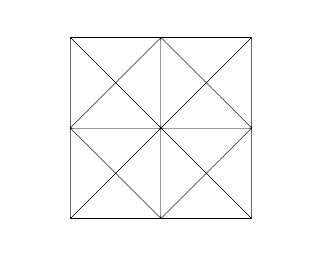
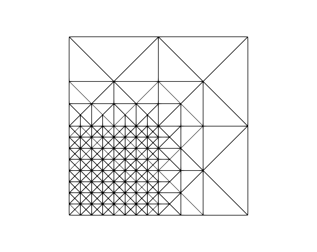
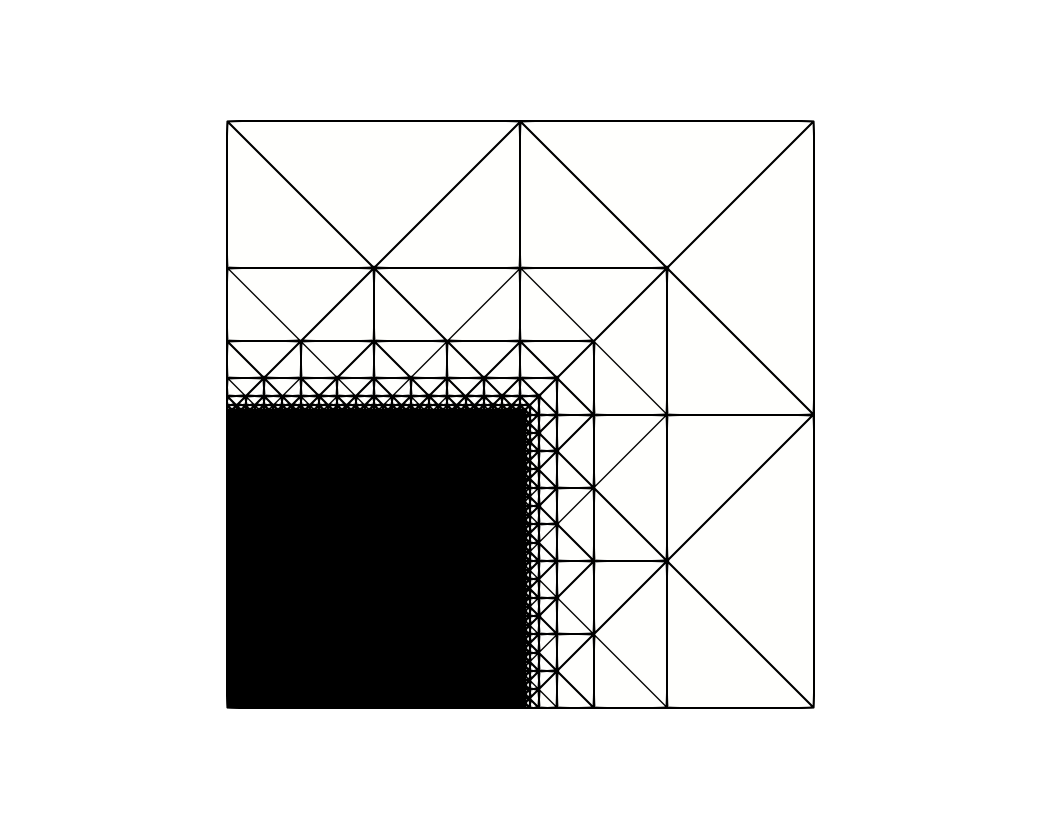
Figure 2. Selection of a sequence of triangulations of $\Omega=(0,1)^{2}$, where in each iteration the elements in $\Omega^{-}=[0,0.5]\times[0,0.5]$ are marked for refinement. The elements $\mathcal{G}^{+}$ in the remaining domain $\Omega\setminus\Omega^{-}$ are, after some iteration, not refined anymore. Moreover, after some iteration, their whole neighbourhood is not refined anymore.

Next, for a fixed $k\in\mathbb{N}_{0}$, we set

$$\mathcal{G}_{k}^{+} :=\mathcal{G}_{k}\cap\mathcal{G}^{+}, \qquad\Omega_{k}^{+} :=\Omega(\mathcal{G}_{k}^{+}),$$

$$\mathcal{G}_{k}^{++} :=\{E\in\mathcal{G}_{k}\colon{N}_{k}(E)\subset\mathcal{G}^{+}\}, \qquad\Omega_{k}^{++} :=\Omega(\mathcal{G}_{k}^{++}),$$

$$\mathcal{G}_{k}^{-} :=\mathcal{G}_{k}\setminus\mathcal{G}_{k}^{++} \qquad\Omega_{k}^{-} :=\Omega(\mathcal{G}_{k}^{-});$$

compare also with Figure 2. This notation is also adopted for the corresponding faces, e.g., we denote $\mathcal{S}_{k}^{+}:=\mathcal{S}(\mathcal{G}_{k}^{+})$ and $\mathring{\mathcal{S}}_{k}^{+}:=\mathring{\mathcal{S}}(\mathcal{G}_{k}^{+})$ and correspondingly for all other above sub-triangulations of $\mathcal{G}_{k}$.

The next lemma states that the meshsize of elements in $\mathcal{G}_{k}^{-}$ converges uniformly to zero; compare also with [MSV08, (4.15) and Corollary 4.1] and [Sie11, Corollary 3.3].

Lemma 11.

We have that $\lim_{k\to\infty}\|h_{k}\chi_{\Omega_{k}^{-}}\|_{L^{\infty}(\Omega)}=0$, with $\chi_{\Omega_{k}^{-}}$ denoting the characteristic function of $\Omega_{k}^{-}$.

In particular, this implies that $\lim_{k\to\infty}|\Omega({N}_{k}(\mathcal{G}^{-}_{k}))\setminus\Omega^{-}|=\lim_{k\to\infty}|\Omega_{k}^{-}\setminus\Omega^{-}|=0$.

Proof.

The first claim is proved in [Sie11, Corollary 3.3].

In order to prove the second claim, we first observe that

$$|\Omega_{k}^{-}\setminus\Omega^{-}|=|\Omega(\mathcal{G}^{+}\setminus\mathcal{G}_{k}^{++})|.$$

For $\ell\in\mathbb{N}$, it follows from Lemma 10 and $\#\mathcal{G}_{\ell}^{+}<\infty$, that there exists $K(\ell)$, such that $\mathcal{G}_{\ell}^{+}\subset\mathcal{G}_{K(\ell)}^{++}$ and thus

(3.1) $$|\Omega(\mathcal{G}^{+}\setminus\mathcal{G}_{K(\ell)}^{++})|\leq|\Omega(\mathcal{G}^{+}\setminus\mathcal{G}_{\ell}^{+})|\to 0\qquad\text{as}\leavevmode\nobreak\ \ell\to\infty,$$

i.e. a subsequence of $\{|\Omega(\mathcal{G}^{+}\setminus\mathcal{G}_{k}^{++})|\}_{k}$ vanishes. However, since the sequence is monotone decreasing, it must vanish as a whole. To conclude, we first realise that $|\Omega({N}_{k}(\mathcal{G}^{-}_{k}))\setminus\Omega^{-}|\leq|\Omega_{k}^{-}\setminus\Omega^{-}|+|\Omega({N}_{k}(\mathcal{G}^{-}_{k})\setminus\mathcal{G}_{k}^{-})|$; it remains to prove that the latter term vanishes as $k\to\infty$. To this end, we observe that

$${N}_{k}(\mathcal{G}^{-}_{k})\setminus\mathcal{G}_{k}^{-}\subset\mathcal{G}_{k}^{++}\setminus\mathcal{G}_{k}^{3+},$$

with $\mathcal{G}_{k}^{3+}=\{E\in\mathcal{G}_{k}\colon{N}_{k}(E)\in\mathcal{G}_{k}^{++}\}$. Indeed, assume that $E\in\mathcal{G}_{k}^{3+}\cap{N}_{k}(\mathcal{G}_{k}^{-})$, then there exists $E^{\prime}\in{N}_{k}(E)$ with $E^{\prime}\in\mathcal{G}_{k}^{++}\cap\mathcal{G}_{k}^{-}$; this is a contradiction. Consequently, we have

$$|\Omega({N}_{k}(\mathcal{G}^{-}_{k})\setminus\mathcal{G}_{k}^{-})|\leq|\Omega(\mathcal{G}_{k}^{++}\setminus\mathcal{G}_{k}^{3+})|\leq|\Omega(\mathcal{G}^{+}\setminus\mathcal{G}_{k}^{3+})|\to 0\quad\text{as}\leavevmode\nobreak\ k\to\infty,$$

where the last limit follows by iterating the reasoning from (3.1). ∎

3.2. The limit space

In this section, we shall investigate the limit of the finite element spaces $\mathbb{V}_{k}:=\mathbb{V}(\mathcal{G}_{k})$, $k\in\mathbb{N}$. To this end, we define

$$\mathbb{V}_{\infty}:=\big{\{}v\in BV(\Omega) :v|_{\Omega^{-}}\in H^{1}_{\partial\Omega\cap\partial\Omega^{-}}(\Omega^{-})\leavevmode\nobreak\ \text{and}\leavevmode\nobreak\ v|_{E}\in\mathbb{P}_{r}\leavevmode\nobreak\ \forall E\in\mathcal{G}^{+}$$

$$\quad\text{such that}\leavevmode\nobreak\ \exists\{v_{k}\}_{k\in\mathbb{N}},v_{k}\in\mathbb{V}_{k}\leavevmode\nobreak\ \text{with}\leavevmode\nobreak\ \limsup_{k\to\infty}\left|\negthinspace\left|\negthinspace\left|{v_{k}}\right|\negthinspace\right|\negthinspace\right|_{k}<\infty$$

$$\quad\text{and}\leavevmode\nobreak\ \lim_{k\to\infty}\left|\negthinspace\left|\negthinspace\left|{v-v_{k}}\right|\negthinspace\right|\negthinspace\right|_{k}+\left\|v-v_{k}\right\|_{\Omega}=0\big{\}};$$

here $H^{1}_{\partial\Omega\cap\partial\Omega^{-}}(\Omega^{-})$ denotes the space of functions from $H_{0}^{1}(\Omega)$ restricted to $\Omega^{-}$. Moreover, we have extended the definition of the piece-wise gradient to

(3.2) $$\nabla_{\!\texttt{pw}}v\in L^{2}(\Omega)^{d}:\quad\nabla_{\!\texttt{pw}}v|_{\Omega^{-}}=\nabla v|_{\Omega^{-}}\quad\text{and}\quad\nabla_{\!\texttt{pw}}v|_{E}=\nabla v|_{E}\leavevmode\nobreak\ \forall E\in\mathcal{G}^{+}.$$

Note that for $v\in BV(\Omega)$ there exists the $L^{1}$-trace of $v$ on $\Gamma_{k}=\bigcup\{S:S\in\mathcal{S}_{k}\}$; compare e.g. with the trace theorem [BO09, Theorem 4.2]. In other words, $v$ is measurable with respect to the $(d-1)$-dimensional Hausdorff measure on $\mathcal{S}_{k}$ and, therefore, the term $\left|\negthinspace\left|\negthinspace\left|{v}\right|\negthinspace\right|\negthinspace\right|_{k}$, $v\in\mathbb{V}_{\infty}$, makes sense. Obviously, we have $\mathbb{V}_{k}\cap C(\Omega)\subset\mathbb{V}_{\infty}$ for all $k\in\mathbb{N}$ and, thus, $\mathbb{V}_{\infty}$ is not empty.

Setting $h_{+}:=h_{\mathcal{G}^{+}}$ and $\mathcal{S}^{+}:=\mathcal{S}(\mathcal{G}^{+})$, we define

$$\left\langle v,\,w\right\rangle_{\infty} :=\int_{\Omega}\nabla_{\!\texttt{pw}}v\cdot\nabla_{\!\texttt{pw}}w\,\mathrm{d}x+\bar{\sigma}\int_{\mathcal{S}^{+}}h_{+}^{-1}\left[\negthinspace\left[{v}\right]\negthinspace\right]\left[\negthinspace\left[{w}\right]\negthinspace\right]\,\mathrm{d}s,$$

and $\left|\negthinspace\left|\negthinspace\left|{v}\right|\negthinspace\right|\negthinspace\right|_{\infty}:=\left\langle v,\,v\right\rangle_{\infty}^{1/2}$, for all $v,w\in\mathbb{V}_{\infty}$.

We shall next list some basic properties of the space $\mathbb{V}_{\infty}$.

Proposition 12.

For $v\in\mathbb{V}_{\infty}$, we have

$$\left|\negthinspace\left|\negthinspace\left|{v}\right|\negthinspace\right|\negthinspace\right|_{k}\nearrow\left|\negthinspace\left|\negthinspace\left|{v}\right|\negthinspace\right|\negthinspace\right|_{\infty}<\infty\quad\text{ as}\leavevmode\nobreak\ k\to\infty.$$

In particular, for fixed $\ell\in\mathbb{N}$, let $E\in\mathcal{G}_{\ell}$; then, we have

$$\int_{\{S\in\mathcal{S}_{k}:S\subset E\}}h_{k}^{-1}\left[\negthinspace\left[{v}\right]\negthinspace\right]^{2}\,\mathrm{d}s\nearrow\int_{\{S\in\mathcal{S}^{+}:S\subset E\}}h_{+}^{-1}\left[\negthinspace\left[{v}\right]\negthinspace\right]^{2}\,\mathrm{d}s,\quad\text{as}\leavevmode\nobreak\ k\to\infty.$$

Proof.

Since $v\in\mathbb{V}_{\infty}$, there exists $\{v_{k}\}_{k\in\mathbb{N}},v_{k}\in\mathbb{V}_{k}$ with $\lim_{k\to\infty}\left|\negthinspace\left|\negthinspace\left|{v-v_{k}}\right|\negthinspace\right|\negthinspace\right|_{k}=0$ and $\limsup_{k\to\infty}\left|\negthinspace\left|\negthinspace\left|{v_{k}}\right|\negthinspace\right|\negthinspace\right|_{k}<\infty$. We first observe that

$$\left|\negthinspace\left|\negthinspace\left|{v}\right|\negthinspace\right|\negthinspace\right|_{k}\leq\left|\negthinspace\left|\negthinspace\left|{v-v_{k}}\right|\negthinspace\right|\negthinspace\right|_{k}+\left|\negthinspace\left|\negthinspace\left|{v_{k}}\right|\negthinspace\right|\negthinspace\right|_{k}<\infty$$

uniformly in $k$. Thanks to the mesh-size reduction, i.e. $h_{m}\leq h_{k}$ for all $m\geq k$, we conclude that

$$\int_{\mathcal{S}_{k}}h_{k}^{-1}\left[\negthinspace\left[{v}\right]\negthinspace\right]^{2}\,\mathrm{d}s\leq\int_{\mathcal{S}_{k}}h_{m}^{-1}\left[\negthinspace\left[{v}\right]\negthinspace\right]^{2}\,\mathrm{d}s\leq\int_{\mathcal{S}_{m}}h_{m}^{-1}\left[\negthinspace\left[{v}\right]\negthinspace\right]^{2}\,\mathrm{d}s,$$

thanks to the inclusion $\bigcup_{\mathcal{S}\in\mathcal{S}_{k}}S\subset\bigcup_{\mathcal{S}\in\mathcal{S}_{m}}S$.

Therefore, we have $\left|\negthinspace\left|\negthinspace\left|{v}\right|\negthinspace\right|\negthinspace\right|_{k}\leq\left|\negthinspace\left|\negthinspace\left|{v}\right|\negthinspace\right|\negthinspace\right|_{m}$ for all $m\geq k$ and, thus, $\{\left|\negthinspace\left|\negthinspace\left|{v}\right|\negthinspace\right|\negthinspace\right|_{k}\}_{k\in\mathbb{N}}$ converges. Consequently, for $\epsilon>0$ there exists $K=K(\epsilon)$, such that for all $k\geq K$ and $m>k$ large enough, we have

$$\epsilon>|\left|\negthinspace\left|\negthinspace\left|{v}\right|\negthinspace\right|\negthinspace\right|_{m}^{2}-\left|\negthinspace\left|\negthinspace\left|{v}\right|\negthinspace\right|\negthinspace\right|_{k}^{2}| =\bar{\sigma}\int_{\mathcal{S}_{m}\setminus(\mathcal{S}_{m}\cap\mathcal{S}_{k})}h_{m}^{-1}\left[\negthinspace\left[{v}\right]\negthinspace\right]^{2}\,\mathrm{d}s-\bar{\sigma}\int_{\mathcal{S}_{k}\setminus(\mathcal{S}_{m}\cap\mathcal{S}_{k})}h_{k}^{-1}\left[\negthinspace\left[{v}\right]\negthinspace\right]^{2}\,\mathrm{d}s$$

$$\geq(2^{1/(d-1)}-1)\,\bar{\sigma}\int_{\mathcal{S}_{k}\setminus(\mathcal{S}_{m}\cap\mathcal{S}_{k})}h_{k}^{-1}\left[\negthinspace\left[{v}\right]\negthinspace\right]^{2}\,\mathrm{d}s$$

$$\geq(2^{1/(d-1)}-1)\,\bar{\sigma}\int_{\mathcal{S}_{k}\setminus\mathcal{S}_{k}^{+}}h_{k}^{-1}\left[\negthinspace\left[{v}\right]\negthinspace\right]^{2}\,\mathrm{d}s.$$

This follows from the fact that $h_{m}|_{S}\leq 2^{-1/(d-1)}h_{k}|_{S}$ for all $S\in\mathcal{S}_{k}\setminus(\mathcal{S}_{m}\cap\mathcal{S}_{k})$ together with $\mathcal{S}_{k}^{+}=\mathcal{S}_{m}\cap\mathcal{S}_{k}$ for sufficiently large $m>k$.

Therefore, we have $\int_{\mathcal{S}_{k}\setminus\mathcal{S}_{k}^{+}}h_{k}^{-1}\left[\negthinspace\left[{v}\right]\negthinspace\right]^{2}\,\mathrm{d}s\to 0$ as $k\to\infty$ and, thus,

$$\left|\negthinspace\left|\negthinspace\left|{v}\right|\negthinspace\right|\negthinspace\right|_{k}^{2} =\int_{\Omega}|\nabla_{\!\texttt{pw}}v|^{2}\,\mathrm{d}x+\bar{\sigma}\int_{\mathcal{S}_{k}^{+}}h_{k}^{-1}\left[\negthinspace\left[{v}\right]\negthinspace\right]^{2}\,\mathrm{d}s+\bar{\sigma}\int_{\mathcal{S}_{k}\setminus\mathcal{S}_{k}^{+}}h_{k}^{-1}\left[\negthinspace\left[{v}\right]\negthinspace\right]^{2}\,\mathrm{d}s\to\left|\negthinspace\left|\negthinspace\left|{v}\right|\negthinspace\right|\negthinspace\right|_{\infty}^{2}+0.$$

This proves the first claim. The second claim is a localised version and follows completely analogously. ∎

As a consequence, we have that Friedrichs and Poincaré inequalities are inherited to $\mathbb{V}_{\infty}$.

Corollary 13 (Friedrichs-$\mathbb{V}_{\infty}$).

We have

$$\left\|v\right\|_{\Omega}\lesssim\left|\negthinspace\left|\negthinspace\left|{v}\right|\negthinspace\right|\negthinspace\right|_{\infty}\quad\text{for all}\leavevmode\nobreak\ v\in\mathbb{V}_{\infty}.$$

Proof.

Since $v\in\mathbb{V}_{\infty}$, there exists $\{v_{k}\}_{k\in\mathbb{N}},v_{k}\in\mathbb{V}_{k}$ with $\limsup_{k\to\infty}\left|\negthinspace\left|\negthinspace\left|{v_{k}}\right|\negthinspace\right|\negthinspace\right|_{k}<\infty$ and $\lim_{k\to\infty}\left|\negthinspace\left|\negthinspace\left|{v-v_{k}}\right|\negthinspace\right|\negthinspace\right|_{k}+\left\|v-v_{k}\right\|_{\Omega}=0$. It thus follows from Corollary 3 and Proposition 12 that

$$\left\|v\right\|_{\Omega}=\lim_{k\to\infty}\left\|v_{k}\right\|_{\Omega}\lesssim\lim_{k\to\infty}\left|\negthinspace\left|\negthinspace\left|{v_{k}}\right|\negthinspace\right|\negthinspace\right|_{k}=\left|\negthinspace\left|\negthinspace\left|{v}\right|\negthinspace\right|\negthinspace\right|_{\infty}.$$

This is the assertion. ∎

Lemma 14 (Poincaré-$\mathbb{V}_{\infty}$).

Fix $k\in\mathbb{N}$ and let $E\in\mathcal{G}_{k}$. Then for $v\in\mathbb{V}_{\infty}$ and $v_{E}:=\frac{1}{|\omega_{k}(E)|}\int_{\omega_{k}(E)}v\,\mathrm{d}x$, we have

$$\left\|v-v_{E}\right\|_{\omega_{k}(E)}^{2}\lesssim\left\|h_{k}\nabla_{\!\texttt{pw}}v\right\|_{\omega_{k}(E)}^{2}+\int_{\{S\in\mathcal{S}^{+}:S\subset\omega_{k}(E)\}}h_{k}^{2}h_{+}^{-1}\left[\negthinspace\left[{v}\right]\negthinspace\right]^{2}\,\mathrm{d}s.$$

Proof.

By the definition of $\mathbb{V}_{\infty}$, there exists $v_{\ell}\in\mathbb{V}_{\ell}$, $\ell\in\mathbb{N}_{0}$, with $\lim_{\ell\to\infty}\left|\negthinspace\left|\negthinspace\left|{v-v_{\ell}}\right|\negthinspace\right|\negthinspace\right|_{\ell}+\left\|v-v_{\ell}\right\|_{\Omega}=0$ and $\limsup_{\ell\to\infty}\left|\negthinspace\left|\negthinspace\left|{v_{\ell}}\right|\negthinspace\right|\negthinspace\right|_{\ell}<\infty$. Therefore, we have

$$\left\|\nabla_{\!\texttt{pw}}v_{\ell}\right\|_{\omega_{k}(E)}^{2}+\int_{\{S\in\mathcal{S}_{\ell}:S\subset\omega_{k}(E)\}}h_{\ell}^{-1}\left[\negthinspace\left[{v_{\ell}}\right]\negthinspace\right]^{2}\,\mathrm{d}s\\ \to\left\|\nabla_{\!\texttt{pw}}v\right\|_{\omega_{k}(E)}^{2}+\int_{\{S\in\mathcal{S}^{+}:S\subset\omega_{k}(E)\}}h_{+}^{-1}\left[\negthinspace\left[{v}\right]\negthinspace\right]^{2}\,\mathrm{d}s\quad\text{as}\leavevmode\nobreak\ \ell\to\infty;$$

see Proposition 12. Moreover, we have

$$\left\|v_{E}-v_{\ell,E}\right\|_{\omega_{k}(E)}\leq\left\|v-v_{\ell}\right\|_{\omega_{k}(E)}\leq\left\|v-v_{\ell}\right\|_{\Omega}\to 0\quad\text{as}\leavevmode\nobreak\ \ell\to\infty,$$

where $v_{\ell,E}:=\frac{1}{|\omega_{k}(E)|}\int_{\omega_{k}(E)}v_{\ell}\,\mathrm{d}x$. We conclude with Proposition 1 that

$$\left\|v-v_{E}\right\|_{\omega_{k}(E)}^{2} \leftarrow\left\|v_{\ell}-v_{\ell,E}\right\|_{\omega_{k}(E)}^{2}$$

$$\lesssim\left\|h_{k}\nabla_{\!\texttt{pw}}v_{\ell}\right\|_{\omega_{k}(E)}^{2}+\int_{\{S\in\mathcal{S}_{\ell}:S\subset\omega_{k}(E)\}}h_{k}^{2}h_{\ell}^{-1}\left[\negthinspace\left[{v_{\ell}}\right]\negthinspace\right]^{2}\,\mathrm{d}s$$

$$\to\left\|h_{k}\nabla_{\!\texttt{pw}}v\right\|_{\omega_{k}(E)}^{2}+\int_{\{S\in\mathcal{S}^{+}:S\subset\omega_{k}(E)\}}h_{k}^{2}h_{+}^{-1}\left[\negthinspace\left[{v}\right]\negthinspace\right]^{2}\,\mathrm{d}s,$$

as $\ell\to\infty$. ∎

In order to extend the dG bilinear form (2.5) to $\mathbb{V}_{\infty}$, we need to define appropriate lifting operators. For each $S\in\mathcal{S}^{+}$, there exists $\ell=\ell(S)\in\mathbb{N}$, such that $S\in\mathcal{S}_{\ell}^{++}$. We define the local lifting operators $R_{\infty}^{S}:L^{2}(S)^{d}\to L^{2}(\Omega)^{d}$ and $L_{\infty}^{S}:L^{2}(S)\to L^{2}(\Omega)^{d}$ by

(3.3) $$R_{\infty}^{S}=R_{\ell}^{S}:=R_{\mathcal{G}_{\ell}}^{S}\qquad\text{and}\qquad L_{\infty}^{S}=L_{\ell}^{S}:=L_{\mathcal{G}_{\ell}}^{S}.$$

From (2.4) it is easy to see, that $R_{\ell}^{S}$ and $L_{\ell}^{S}$ depend only on $S$ and the at most two adjacent elements $E,E^{\prime}\in\mathcal{G}_{\ell}^{+}$ with $S\subset E\cap E^{\prime}$. Therefore, and thanks to the fact that the $\mathcal{G}_{k}^{+}$ are nested, we have that $R_{\ell}^{S}=R_{k}^{S}$ for all $k\geq\ell$ and, thus, the definition is unique. We formally define the global lifting operators by

$$R_{\infty}:=\sum_{S\in\mathcal{S}^{+}}R_{\infty}^{S}\qquad\text{and}\qquad L_{\infty}:=\sum_{S\in\mathring{\mathcal{S}}^{+}}L_{\infty}^{S};$$

here $\mathring{\mathcal{S}}^{+}:=\{S\in\mathcal{S}^{+}:S\not\in\partial\Omega\}$.

Moreover, from the local estimates (2.4c), it is easy to see that for $v\in\mathbb{V}_{\infty}$ and $\boldsymbol{\beta}\in\mathbb{R}^{d}$, we have that $\sum_{S\in\mathcal{S}_{k}^{+}}R_{\infty}^{S}(\left[\negthinspace\left[{v}\right]\negthinspace\right])$ and $\sum_{S\in\mathring{\mathcal{S}}_{k}^{+}}L_{\infty}^{S}(\boldsymbol{\beta}\cdot\left[\negthinspace\left[{v}\right]\negthinspace\right])$ are Cauchy sequences in $L^{2}(\Omega)^{d}$. Consequently, $R_{\infty}(\left[\negthinspace\left[{v}\right]\negthinspace\right]),L_{\infty}(\boldsymbol{\beta}\cdot\left[\negthinspace\left[{v}\right]\negthinspace\right])\in L^{2}(\Omega)$ are well posed and we have

(3.4) $$\left\|R_{\infty}(\left[\negthinspace\left[{v}\right]\negthinspace\right])\right\|_{\Omega}\lesssim\left\|h_{+}^{-1/2}v\right\|_{\Gamma^{+}}\quad\text{and}\quad\left\|L_{\infty}(\boldsymbol{\beta}\cdot\left[\negthinspace\left[{v}\right]\negthinspace\right])\right\|_{\Omega}\lesssim\left|\boldsymbol{\beta}\right|\left\|h_{+}^{-1/2}v\right\|_{\mathring{\Gamma}^{+}},$$

where $\Gamma^{+}=\bigcup\{S:S\in\mathcal{S}^{+}\}$ and $\mathring{\Gamma}^{+}=\bigcup\{S:S\in\mathring{\mathcal{S}}^{+}\}$. This enables us to generalise the discontinuous Galerkin bilinear form to $\mathbb{V}_{\infty}$ setting

$$\mathfrak{B}_{\infty}[w,\,v] :=\int_{\Omega}\nabla_{\!\texttt{pw}}w\cdot\nabla_{\!\texttt{pw}}v\,\mathrm{d}x-\int_{\mathcal{S}^{+}}\big{(}\{\kern-4.55244pt\{\nabla w\}\kern-4.55244pt\}\cdot\left[\negthinspace\left[{v}\right]\negthinspace\right]+\theta\{\kern-4.55244pt\{\nabla v\}\kern-4.55244pt\}\cdot\left[\negthinspace\left[{w}\right]\negthinspace\right]\big{)}\,\mathrm{d}s$$

$$\quad+\int_{\mathring{\mathcal{S}}^{+}}\big{(}\boldsymbol{\beta}\cdot\left[\negthinspace\left[{w}\right]\negthinspace\right]\left[\negthinspace\left[{\nabla v}\right]\negthinspace\right]+\left[\negthinspace\left[{\nabla w}\right]\negthinspace\right]\boldsymbol{\beta}\cdot\left[\negthinspace\left[{v}\right]\negthinspace\right]\big{)}\,\mathrm{d}s$$

$$\quad+\int_{\Omega}\gamma\big{(}R_{\infty}(\left[\negthinspace\left[{w}\right]\negthinspace\right])+L_{\infty}(\boldsymbol{\beta}\cdot\left[\negthinspace\left[{w}\right]\negthinspace\right])\big{)}\cdot\big{(}R_{\infty}(\left[\negthinspace\left[{v}\right]\negthinspace\right])+L_{\infty}(\boldsymbol{\beta}\cdot\left[\negthinspace\left[{v}\right]\negthinspace\right])\big{)}\,\mathrm{d}x$$

$$\quad+\int_{\mathcal{S}^{+}}\frac{\sigma}{h_{+}}\left[\negthinspace\left[{w}\right]\negthinspace\right]\cdot\left[\negthinspace\left[{v}\right]\negthinspace\right]\,\mathrm{d}s,$$

for $v,w\in\mathbb{V}_{\infty}$.

Lemma 15.

The space $\big{(}\mathbb{V}_{\infty},\left\langle\cdot,\,\cdot\right\rangle_{\infty}\big{)}$ is a Hilbert space.

Corollary 16.

There exists a unique $u_{\infty}\in\mathbb{V}_{\infty}$, such that

(3.5) $$\mathfrak{B}_{\infty}[u_{\infty},\,v]=\int_{\Omega}fv\,\mathrm{d}x\qquad\text{for all}\leavevmode\nobreak\ v\in\mathbb{V}_{\infty}.$$

In order to prove the last two statements, we introduce a new quasi-interpolation, which is designed in due consideration of the future refinements. The proofs of Lemma 15 and Corollary 16 are postponed to the end of Section 3.3.

3.3. Quasi-interpolation

We shall now define a quasi-interpolation operator $\Pi_{k}$, which maps into $\mathbb{V}_{\infty}\cap\mathbb{V}_{k}$; this will be a key technical tool in the analysis. On the one hand, membership in $\mathbb{V}_{\infty}\cap\mathbb{V}_{k}$ suggests to use some Clément type interpolation since the mapped functions need to be continuous in $\Omega^{-}$. On the other hand, the fact that the ADGM may leave some elements (namely $\mathcal{G}_{k}^{+}\supset\mathcal{G}_{k}^{++}$) unrefined, suggests to define $\Pi_{k}$ to be the identity on these elements. Note that the quasi-interpolation operator from [CGS13] is motivated by a similar idea in order to map from one Crouzeix-Raviart space into its intersection with a finer one.

For fixed $k\in\mathbb{N}$, let $\{\Phi_{z}^{E}:E\in\mathcal{G}_{k},\leavevmode\nobreak\ z\in\mathcal{N}_{k}(E)\}$ be the Lagrange basis of $\mathbb{V}_{k}:=\mathbb{V}(\mathcal{G}_{k})$, i.e., $\Phi_{z}^{E}$ is a piecewise polynomial of degree $r$ with $\operatorname{supp}(\Phi_{z}^{E})=E$ and

$$\Phi_{z}^{E}(y)=\delta_{zy}\qquad\text{for all}\leavevmode\nobreak\ z,y\in\mathcal{N}_{k}.$$

Its dual basis is then the set $\{\Psi_{z}^{E}:E\in\mathcal{G}_{k},\leavevmode\nobreak\ z\in\mathcal{N}_{k}(E)\}$ of piecewise polynomials of degree $r$, such that $\operatorname{supp}(\Psi_{z}^{E})=E$ and

$$\left\langle\Psi_{y}^{E},\,\Phi_{z}^{E}\right\rangle_{\Omega}=\delta_{zy}\qquad\text{for all}\leavevmode\nobreak\ z,y\in\mathcal{N}_{k}(E).$$

For all $\ell\geq k$, we define $\Pi_{k}:L^{1}(\Omega)\to L^{1}(\Omega)$ by

(3.6) $$\Pi_{k}v:=\sum_{E\in\mathcal{G}_{k}}\sum_{z\in\mathcal{N}_{k}(E)}(\Pi_{k}v)|_{E}(z)\,\Phi_{z}^{E},$$

where for $z\in\mathcal{N}_{k}(E)$ we have that

(3.7) $$(\Pi_{k}v)|_{E}(z):=\begin{cases}\int_{E}v\Psi_{z}^{E}\,\mathrm{d}x,\quad&\text{if}\leavevmode\nobreak\ {N}_{k}(z)\cap\mathcal{G}_{k}^{++}\neq\emptyset\\ 0,\quad&\text{else if}\leavevmode\nobreak\ z\in\partial\Omega\\ \sum_{E^{\prime}\in{N}_{k}(z)}\frac{|E^{\prime}|}{|\omega_{k}(z)|}\int_{E^{\prime}}v\Psi_{z}^{E^{\prime}}\,\mathrm{d}x,\quad&\text{else.}\end{cases}$$

Beyond standard stability and interpolation estimates for $H_{0}^{1}(\Omega)$ functions [SZ90, DG12], we list the following properties related to our setting.

Lemma 17 (Properties of $\Pi_{k}$).

The operator $\Pi_{k}:L^{1}(\Omega)\to L^{1}(\Omega)$ defined in (3.6) has the following properties:

1. $\Pi_{k}:L^{p}(\Omega)\to L^{p}(\Omega)$ is a linear and bounded projection for all $1\leq p\leq\infty$. In particular, we have that

   $$\left\|\Pi_{k}v\right\|_{L^{p}(E)}\lesssim\left\|v\right\|_{L^{p}(\omega_{k}(E))},$$

   where the constant solely depends on $p$, $r$, $d$, and the shape regularity of $\mathcal{G}_{0}$.

2. $\Pi_{k}v\in\mathbb{V}_{k}$ for all $v\in L^{1}(\Omega)$;

3. $\Pi_{k}v|_{E}=v|_{E}$, if $E\in\mathcal{G}_{k}$ and $v|_{\omega_{k}(E)}\in\mathbb{P}_{r}(\omega_{k}(E))$;

4. $\Pi_{k}v|_{E}=v|_{E}$, if $E\in\mathcal{G}_{k}^{++}$ and $v|_{E}\in\mathbb{P}_{r}(E)$; if moreover $v\in\mathbb{V}_{k}$, then also $\left[\negthinspace\left[{v-\Pi_{k}v}\right]\negthinspace\right]|_{S}\equiv 0$ for all $S\in\mathcal{S}_{k}^{++}$.

5. $\Pi_{k}v|_{\Omega\setminus\Omega_{k}^{+}}\in C(\overline{\Omega\setminus\Omega_{k}^{+}})$ and $\left[\negthinspace\left[{\Pi_{k}v}\right]\negthinspace\right]=0$ on $\partial(\Omega\setminus\Omega^{+}_{k})$;

6. $\Pi_{k}v=v$, for all $v\in\mathbb{V}_{k}$ with $v|_{\Omega\setminus\Omega_{k}^{++}}\in C(\Omega\setminus\Omega_{k}^{++})$;

7. $\Pi_{k}v\in\mathbb{V}_{\infty}$, and we have $\left|\negthinspace\left|\negthinspace\left|{\Pi_{k}v}\right|\negthinspace\right|\negthinspace\right|_{k}=\left|\negthinspace\left|\negthinspace\left|{\Pi_{k}v}\right|\negthinspace\right|\negthinspace\right|_{\infty}$.

Proof.

Claims (1)–(3) follow by standard estimates for the Scott-Zhang operator [SZ90, DG12].

Assertion (4) is a consequence of the definition (3.7) of $\Pi_{k}$ since $E\in\mathcal{G}_{k}^{++}$ implies that ${N}_{k}(E)\cap\mathcal{G}_{k}^{++}={N}_{k}(E)$. Note that $v\in\mathbb{V}(\mathcal{G})$ implies $v|_{E}\in\mathbb{P}_{r}(E)$ for all $E\in\mathcal{G}_{k}$ and thus $(\Pi_{k}v)|_{E}(z)=v|_{E}(z)$ for all $E\in{N}_{k}(z)$ if ${N}_{k}(z)\cap\mathcal{G}_{k}^{++}\neq\emptyset$. This is in particular the case when $z\in S\cap\mathcal{N}_{k}$ with $S\in\mathcal{S}_{k}^{++}$.

For $E\in\mathcal{G}_{k}\setminus\mathcal{G}_{k}^{+}$, we have that ${N}_{k}(z)\cap\mathcal{G}_{k}^{++}=\emptyset$ since otherwise there exists $E^{\prime}\in{N}_{k}(E)\cap\mathcal{G}_{k}^{++}$ and thus $E\in{N}_{k}(E^{\prime})$, which implies $E\in\mathcal{G}_{k}^{+}$, thanks to the definition of $\mathcal{G}_{k}^{++}$. Therefore, (3.7) implies that $\Pi_{k}v$ is continuous on $\Omega\setminus\Omega_{k}^{+}$. Moreover, for $z\in\mathcal{N}_{k}(E)\cap\Omega\setminus\Omega^{+}_{k}$, definition (3.7) is independent of $E$ and thus $\Pi_{k}v$ does not jump across the boundary $\Omega\setminus\Omega_{k}^{+}$. This completes the proof of (5).

On the one hand, if $v\in\mathbb{V}_{k}$ with $v|_{\Omega\setminus\Omega_{k}^{+}}\in C(\overline{\Omega\setminus\Omega_{k}^{++}})$ then we have clearly $\Pi_{k}v|_{\Omega\setminus\Omega_{k}^{+}}=v|_{\Omega\setminus\Omega_{k}^{+}}$. On the other hand, we can conclude $\Pi_{k}v|_{\Omega_{k}^{++}}=v|_{\Omega_{k}^{++}}$ from (4). This yields (6).

The claim (7) is an immediate consequence of (5). ∎

Lemma 18 (Stability).

Let $v\in\mathbb{V}_{\ell}$ for some $k\leq\ell\in\mathbb{N}_{0}\cup\{\infty\}$. Then for all $E\in\mathcal{G}_{k}$, we have

$$\int_{E}\left|\nabla\Pi_{k}v\right|^{2}\,\mathrm{d}x+\int_{\partial E}h_{k}^{-1}\left[\negthinspace\left[{\Pi_{k}v}\right]\negthinspace\right]^{2}\,\mathrm{d}s\\ \lesssim\int_{\omega_{k}(E)}\left|\nabla_{\!\texttt{pw}}v\right|^{2}\,\mathrm{d}x+\sum_{E^{\prime}\in\mathcal{G}_{\ell},E^{\prime}\subset\omega_{k}(E)}\int_{\partial E^{\prime}}h_{\ell}^{-1}\left[\negthinspace\left[{v}\right]\negthinspace\right]^{2}\,\mathrm{d}s,$$

setting $\mathcal{G}_{\ell}:=\mathcal{G}^{+}$ and $h_{\ell}:=h_{+}$, when $\ell=\infty$. In particular, we have $\left|\negthinspace\left|\negthinspace\left|{\Pi_{k}v}\right|\negthinspace\right|\negthinspace\right|_{k}\lesssim\left|\negthinspace\left|\negthinspace\left|{v}\right|\negthinspace\right|\negthinspace\right|_{\ell}$.

Proof.

We begin by noting that, summing over all elements in $\mathcal{G}_{k}$ and accounting for the finite overlap of the domains $\omega_{k}(E)$, $E\in\mathcal{G}_{k}$, the global stability estimate is an immediate consequence of the corresponding local one.

We first assume $\ell<\infty$. Let $E\in\mathcal{G}_{k}^{++}\subset\mathcal{G}_{\ell}^{++}$. Then, thanks to Lemma 17(4), we have $\Pi_{k}v|_{E}=v|_{E}$. Moreover, let $E^{\prime}\in\mathcal{G}_{k}$ such that $E\cap E^{\prime}\in\mathcal{S}_{k}$; then ${N}_{k}(z)\ni E\in\mathcal{G}_{k}^{++}$ and thus $(\Pi_{k}v)|_{E^{\prime}}(z)=v|_{E^{\prime}}(z)$, for all $z\in\mathcal{N}_{k}(E)\cap\mathcal{N}_{k}(E^{\prime})$. Consequently, we have $\left[\negthinspace\left[{\Pi_{k}v}\right]\negthinspace\right]=\left[\negthinspace\left[{v}\right]\negthinspace\right]$ on $\partial E$, in other words

(3.8) $$\int_{E}\left|\nabla\Pi_{k}v\right|^{2}\,\mathrm{d}x+\int_{\partial E}h_{k}^{-1}\left[\negthinspace\left[{\Pi_{k}v}\right]\negthinspace\right]^{2}\,\mathrm{d}s=\int_{E}\left|\nabla v\right|^{2}\,\mathrm{d}x+\int_{\partial E}h_{k}^{-1}\left[\negthinspace\left[{v}\right]\negthinspace\right]^{2}\,\mathrm{d}s.$$

Let now $E\in\mathcal{G}_{k}$ be arbitrary. Then, an inverse estimate and the local stability (Lemma 17 (1) and (3)) for $v_{E}:=\frac{1}{|\omega_{k}(E)|}\int_{\omega_{k}(E)}v\,\mathrm{d}x\in\mathbb{R}$, imply

(3.9) $$\begin{aligned} \int_{E}\left|\nabla\Pi_{k}v\right|^{2}\,\mathrm{d}x&\lesssim\int_{E}h_{k}^{-2}\left|\Pi_{k}(v-v_{E})\right|^{2}\,\mathrm{d}x\lesssim\int_{\omega_{k}(E)}h_{k}^{-2}\left|v-v_{E}\right|^{2}\,\mathrm{d}x\\ &\lesssim\sum_{E^{\prime}\subset\omega_{k}(E),E^{\prime}\in\mathcal{G}_{\ell}}\int_{E^{\prime}}\left|\nabla v\right|^{2}\,\mathrm{d}x+\int_{\partial E^{\prime}}h_{\ell}^{-1}\left[\negthinspace\left[{v}\right]\negthinspace\right]^{2}\,\mathrm{d}s;\end{aligned}$$

here the last estimate follows from the broken Poincaré inequality, Proposition 1.

If now for all $E^{\prime}\in\mathcal{G}_{k}$, with $E^{\prime}\subset\omega_{k}(E)$, we have $E^{\prime}\not\in\mathcal{G}_{k}^{++}$, which implies $E\in\mathcal{G}_{k}\setminus\mathcal{G}_{k}^{++}$. Then, thanks to Lemma 17(5), we have that $\Pi_{k}v$ is continuous across $\partial E$, i.e., $\left[\negthinspace\left[{\Pi_{k}v}\right]\negthinspace\right]|_{\partial E}=0$. On the contrary, assuming that there exists $E^{\prime}\in\mathcal{G}_{k}^{++}$, with $E^{\prime}\in{N}_{k}(E)$, we conclude that $E\in{N}_{k}(E^{\prime})$ and thus $E\in\mathcal{G}^{+}$. From the local quasi uniformity, we thus have for all $E^{\prime\prime}\in\mathcal{G}_{\ell}$ with $E^{\prime\prime}\cap E\neq\emptyset$ that $|E^{\prime\prime}|\eqsim|E|$. Let $z\in\mathcal{N}_{k}(E)$; then, according to (3.7), we have that

$$\left[\negthinspace\left[{\Pi_{k}v}\right]\negthinspace\right]|_{\partial E}(z)=\begin{cases}\left[\negthinspace\left[{v}\right]\negthinspace\right]|_{\partial E}(z),\quad&\text{if}\leavevmode\nobreak\ \exists E^{\prime}\in{N}_{k}(z)\cap\mathcal{G}_{k}^{++};\\ 0,&\text{else.}\end{cases}$$

Using standard scaling arguments, this implies

$$\int_{\partial E}\left[\negthinspace\left[{\Pi_{k}v}\right]\negthinspace\right]^{2}\,\mathrm{d}s \eqsim|\partial E|\sum_{z\in\mathcal{N}_{k}\cap\partial E}\big{(}\left[\negthinspace\left[{\Pi_{k}v}\right]\negthinspace\right]|_{\partial E}(z)\big{)}^{2}=|\partial E|\sum_{z\in\mathcal{N}_{k}\cap\partial E}\big{(}\left[\negthinspace\left[{v}\right]\negthinspace\right]|_{\partial E}(z)\big{)}^{2}$$

$$\leq|\partial E|\sum_{z\in\mathcal{N}_{\ell}\cap\partial E}\big{(}\left[\negthinspace\left[{v}\right]\negthinspace\right]|_{\partial E}(z)\big{)}^{2}\eqsim\int_{\partial E}\left[\negthinspace\left[{v}\right]\negthinspace\right]^{2}\,\mathrm{d}s.$$

Combining this with (3.9) proves the local bound in the case $\ell<\infty$.

For $\ell=\infty$, we observe that a bound similar to (3.9) can be obtained with Lemma 14 instead of Proposition 1. The local bound follows then by arguing as in the case $\ell<\infty$. ∎

Corollary 19 (Interpolation estimate).

For $v\in\mathbb{V}_{\ell}$, $k\leq\ell\in\mathbb{N}\cup\{\infty\}$, we have that

$$\int_{E}|\nabla_{\!\texttt{pw}}v-\nabla_{\!\texttt{pw}}\Pi_{k}v|^{2}\,\mathrm{d}x+\int_{E}h_{k}^{-2}|v-\Pi_{k}v|^{2}+\int_{\partial E}h_{k}^{-1}\left[\negthinspace\left[{v-\Pi_{k}v}\right]\negthinspace\right]^{2}\\ \lesssim\int_{\omega_{k}(E)}|\nabla_{\!\texttt{pw}}v|^{2}\,\mathrm{d}x+\sum_{S\in\mathcal{S}_{\ell},S\subset\omega_{k}(E)}\int_{S}h_{k}^{-1}\left[\negthinspace\left[{v}\right]\negthinspace\right]^{2},$$

where we set $\mathcal{G}_{\ell}:=\mathcal{G}^{+}$ and $h_{\ell}:=h_{+}$, when $\ell=\infty$. The constant depends only on $d$, $r$ and the shape regularity of $\mathcal{G}_{0}$.

Proof.

The claim follows from Lemma 17(3), together with the stability Lemma 18 and the local Poincaré inequality from Proposition 1, respectively, Lemma 14. ∎

The next result concerns the convergence of the quasi-interpolation.

Lemma 20.

Let $v\in\mathbb{V}_{\infty}$; then,

$$\left|\negthinspace\left|\negthinspace\left|{v-\Pi_{k}v}\right|\negthinspace\right|\negthinspace\right|_{k}\to 0\qquad\text{and}\qquad\left|\negthinspace\left|\negthinspace\left|{v-\Pi_{k}v}\right|\negthinspace\right|\negthinspace\right|_{\infty}\to 0$$

as $k\to\infty$.

Proof.

For brevity, set $v_{k}:=\Pi_{k}v\in\mathbb{V}_{k}$. Thanks to Lemma 14 and Lemma 17(4) and (5), we have that

$$\left|\negthinspace\left|\negthinspace\left|{v-v_{k}}\right|\negthinspace\right|\negthinspace\right|_{k}^{2} \lesssim\int_{\mathcal{G}_{k}\setminus\mathcal{G}_{k}^{++}}|\nabla_{\!\texttt{pw}}v-\nabla_{\!\texttt{pw}}v_{k}|^{2}\,\mathrm{d}x+\int_{\mathcal{S}_{k}\setminus\mathcal{S}_{k}^{++}}h_{k}^{-1}\left|\left[\negthinspace\left[{v-v_{k}}\right]\negthinspace\right]\right|^{2}\,\mathrm{d}s$$

$$\leq\int_{\mathcal{G}_{k}^{-}}|\nabla_{\!\texttt{pw}}v-\nabla_{\!\texttt{pw}}v_{k}|^{2}\,\mathrm{d}x+\int_{\mathcal{S}_{k}^{-}}h_{k}^{-1}\left|\left[\negthinspace\left[{v-v_{k}}\right]\negthinspace\right]\right|^{2}\,\mathrm{d}s$$

$$=I^{-}_{k}+II^{-}_{k}.$$

We conclude from Lemma 18 that

$$II^{-}_{k} =\int_{\mathcal{S}_{k}^{-}}h_{k}^{-1}\left|\left[\negthinspace\left[{v-v_{k}}\right]\negthinspace\right]\right|^{2}\,\mathrm{d}s\lesssim\sum_{E\in\mathcal{G}_{k}^{-}}\sum_{E^{\prime}\in\mathcal{G}^{+},E^{\prime}\subset\omega_{k}(E)}\leavevmode\nobreak\ \int_{\partial E^{\prime}}h_{+}^{-1}\left[\negthinspace\left[{v}\right]\negthinspace\right]^{2}\,\mathrm{d}s$$

$$\lesssim\int_{\mathcal{S}^{+}\setminus\mathcal{S}_{k}^{++}}h_{+}^{-1}\left[\negthinspace\left[{v}\right]\negthinspace\right]^{2}\,\mathrm{d}s.$$

The term on the right hand side is the tail of a convergent series, since it is bounded thanks to $\left|\negthinspace\left|\negthinspace\left|{v}\right|\negthinspace\right|\negthinspace\right|_{\infty}<\infty$ and all of its summands are positive. Therefore, $II_{k}^{-}\to 0$ as $k\to\infty$.

Thus, it remains to prove that $I_{k}^{-}\to 0$ as $k\to\infty$. To this end, we recall that thanks to the definition of $H^{1}_{\partial\Omega\cap\partial\Omega^{-}}(\Omega^{-})$ we have that $v|_{\Omega^{-}}=\tilde{v}|_{\Omega^{-}}$ for some function $\tilde{v}\in H_{0}^{1}(\Omega)$. Since $H_{0}^{2}(\Omega)$ is dense in $H_{0}^{1}(\Omega)$, for $\epsilon>0$, there exists $v_{\epsilon}\in H^{2}_{0}(\Omega)$ such that $\|\tilde{v}-v_{\epsilon}\|_{H^{1}(\Omega^{-})}\leq\|\tilde{v}-v_{\epsilon}\|_{H^{1}(\Omega)}<\epsilon$. Combining Lemma 17(3) and (1) with standard estimates [SZ90, DG12] for $H_{0}^{1}(\Omega)$ functions, with the Bramble-Hilbert Lemma (see, e.g., [BS02]), we obtain

$$\int_{\mathcal{G}_{k}^{-}}|\nabla_{\!\texttt{pw}}v-\nabla v_{k}|^{2}\,\mathrm{d}x\\ \begin{aligned} &\lesssim\int_{\mathcal{G}_{k}^{-}}|\nabla v_{\epsilon}-\nabla\Pi_{k}v_{\epsilon}|^{2}+|\nabla_{\!\texttt{pw}}(v-v_{\epsilon})-\nabla\Pi_{k}(v-v_{\epsilon})|^{2}\,\mathrm{d}x\\ &\lesssim\int_{{N}_{k}(\mathcal{G}_{k}^{-})}h_{k}^{2}\sum_{|\alpha|=2}|D^{\alpha}v_{\epsilon}|^{2}\,\mathrm{d}x+\int_{{N}_{k}(\mathcal{G}_{k}^{-})}|\nabla_{\!\texttt{pw}}(v-v_{\epsilon})|^{2}\,\mathrm{d}x\\ &\lesssim\|h_{k}\chi_{\Omega_{k}^{-}}\|_{L^{\infty}(\Omega)}^{2}\int_{\Omega}\sum_{|\alpha|=2}|D^{\alpha}v_{\epsilon}|^{2}\,\mathrm{d}x+\int_{{N}_{k}(\mathcal{G}_{k}^{-})}|\nabla_{\!\texttt{pw}}(v-v_{\epsilon})|^{2}\,\mathrm{d}x,\end{aligned}$$

where we have used that $\|h_{k}\|_{L^{\infty}(\Omega({N}_{k}(\mathcal{G}_{k}^{-})))}\lesssim\|h_{k}\chi_{\Omega_{k}^{-}}\|_{L^{\infty}(\Omega)}\to 0$ as $k\to\infty$, thanks to the local quasi-uniformity of $\mathcal{G}_{k}$ and Lemma 11. Moreover, we conclude $\int_{{N}_{k}(\mathcal{G}_{k}^{-})}|\nabla_{\!\texttt{pw}}(v-v_{\epsilon})|^{2}\,\mathrm{d}x\rightarrow\int_{\Omega^{-}}|\nabla(v-v_{\epsilon})|^{2}\,\mathrm{d}x<\epsilon$ from Lemma 11 and the absolute continuity of the Lebesgue integral. Consequently, $\lim_{k\to\infty}I^{-}_{k}\lesssim\epsilon$, which completes the proof of the first claim, since $\epsilon>0$ is arbitrary.

The second claim follows similarly by replacing $\mathcal{S}_{k}$ by $\mathcal{S}^{+}$ and noting that $\left|\negthinspace\left|\negthinspace\left|{\Pi_{k}v}\right|\negthinspace\right|\negthinspace\right|_{k}=\left|\negthinspace\left|\negthinspace\left|{\Pi_{k}v}\right|\negthinspace\right|\negthinspace\right|_{\infty}$, since $\Pi_{k}v$ is continuous in $\Omega\setminus\Omega^{+}$. ∎

Proof of Lemma 15.

The positivity of $\left|\negthinspace\left|\negthinspace\left|{\cdot}\right|\negthinspace\right|\negthinspace\right|_{\infty}$ on $\mathbb{V}_{\infty}$ follows from Lemma 20 together with Corollary 13.

In order to prove that $\mathbb{V}_{\infty}$ is complete with respect to $\left|\negthinspace\left|\negthinspace\left|{\cdot}\right|\negthinspace\right|\negthinspace\right|_{\infty}$, let $\{v^{\ell}\}_{\ell\in\mathbb{N}}\subset\mathbb{V}_{\infty}$ be a Cauchy sequence with respect to $\left|\negthinspace\left|\negthinspace\left|{\cdot}\right|\negthinspace\right|\negthinspace\right|_{\infty}$. Note that thanks to the Friedrichs inequality (Corollary 13), there exists the limit $v^{\ell}\to v\in L^{2}(\Omega)$; this is the candidate for the limit of $v^{\ell}$ in $\mathbb{V}_{\infty}$.

We first observe that, since $v^{\ell}|_{E}\in\mathbb{P}_{r}$ for all $E\in\mathcal{G}^{+}$, it follows from the definition of $\left|\negthinspace\left|\negthinspace\left|{\cdot}\right|\negthinspace\right|\negthinspace\right|_{\infty}$ that $v|_{E}\in\mathbb{P}_{r}$ for all $E\in\mathcal{G}^{+}$. Moreover, Propositions 4 and 20 imply that $\{v^{\ell}\}_{\ell\in\mathbb{N}}$ is also a Cauchy Sequence in $BV(\Omega)$ and thus $v\in BV(\Omega)$. Therefore, $v$ has $L^{1}$-traces on each $\partial E$, $E\in\mathcal{G}_{k}$, $k\in\mathbb{N}$.

Next, we deal with the jump terms. To this end, we first observe that, for $k\in\mathbb{N}$, $\{v^{\ell}\}_{\ell\in\mathbb{N}}$ is also a Cauchy sequence with respect to the $\left|\negthinspace\left|\negthinspace\left|{\cdot}\right|\negthinspace\right|\negthinspace\right|_{k}$-norm and uniqueness of limits imply $\left[\negthinspace\left[{v^{\ell}}\right]\negthinspace\right]|_{S}\to\left[\negthinspace\left[{v}\right]\negthinspace\right]|_{S}$ in $L^{2}(S)$ as $\ell\to\infty$, for all $S\in\mathcal{S}_{k}$, in the sense of traces. Let $\epsilon>0$ arbitrary fixed, then there exists $L=L(\epsilon)$, such that $\left|\negthinspace\left|\negthinspace\left|{v^{j}-v^{\ell}}\right|\negthinspace\right|\negthinspace\right|_{k}\leq\left|\negthinspace\left|\negthinspace\left|{v^{j}-v^{\ell}}\right|\negthinspace\right|\negthinspace\right|_{\infty}\leq\epsilon$ for all $j\geq\ell\geq L$. Fix $\ell\geq L$, then thanks to Proposition 12, there exists $K\equiv K(\epsilon,L)$, such that for all $k\geq K$, we have

$$\int_{\mathcal{S}_{k}\setminus\mathcal{S}_{k}^{+}}h_{+}^{-1}\left[\negthinspace\left[{v^{L}}\right]\negthinspace\right]^{2}\,\mathrm{d}s\leq\epsilon^{2}.$$

Consequently, we have

$$\begin{aligned} \int_{\mathcal{S}_{k}}h_{k}^{-1}\left[\negthinspace\left[{v}\right]\negthinspace\right]^{2}\,\mathrm{d}s&=\int_{\mathcal{S}_{k}\setminus\mathcal{S}_{k}^{+}}h_{k}^{-1}\left[\negthinspace\left[{v}\right]\negthinspace\right]^{2}\,\mathrm{d}s+\int_{\mathcal{S}_{k}^{+}}h_{k}^{-1}\left[\negthinspace\left[{v}\right]\negthinspace\right]^{2}\,\mathrm{d}s\\ &=\lim_{\ell\to\infty}\int_{\mathcal{S}_{k}\setminus\mathcal{S}_{k}^{+}}h_{k}^{-1}\left[\negthinspace\left[{v^{\ell}}\right]\negthinspace\right]^{2}\,\mathrm{d}s+\int_{\mathcal{S}_{k}^{+}}h_{k}^{-1}\left[\negthinspace\left[{v}\right]\negthinspace\right]^{2}\,\mathrm{d}s.\end{aligned}$$

Thus, it follows from

(3.10) $$\int_{\mathcal{S}_{k}\setminus\mathcal{S}_{k}^{+}}h_{k}^{-1}\left[\negthinspace\left[{v^{\ell}}\right]\negthinspace\right]^{2}\,\mathrm{d}s\leq 2\left|\negthinspace\left|\negthinspace\left|{v^{\ell}-v^{L}}\right|\negthinspace\right|\negthinspace\right|_{k}^{2}+2\int_{\mathcal{S}_{k}\setminus\mathcal{S}_{k}^{+}}h_{k}^{-1}\left[\negthinspace\left[{v^{L}}\right]\negthinspace\right]^{2}\,\mathrm{d}s\leq 4\epsilon^{2},$$

for $\ell\geq L$, that

(3.11) $$\int_{\mathcal{S}_{k}}h_{k}^{-1}\left[\negthinspace\left[{v}\right]\negthinspace\right]^{2}\,\mathrm{d}s\to\int_{\mathcal{S}^{+}}h_{+}^{-1}\left[\negthinspace\left[{v}\right]\negthinspace\right]^{2}\,\mathrm{d}s\qquad\text{as}\leavevmode\nobreak\ k\to\infty,$$

since $\epsilon>0$ is arbitrary.

We next verify that $v|_{\Omega^{-}}\in H^{1}_{\partial\Omega\cap\partial\Omega^{-}}(\Omega^{-})$, i.e., that $v$ is a restriction of a function from $H_{0}^{1}(\Omega)$ to $\Omega^{-}$. To this end, for each $\ell,m\in\mathbb{N}$, we define $v^{\ell}_{m}:=\Pi_{m}v^{\ell}\in\mathbb{V}_{m}$ for $\ell\geq m\in\mathbb{N}$ and since $v^{\ell}_{m}\in C(\Omega\setminus\Omega^{+}_{k})\subset C(\Omega\setminus\Omega^{+}_{m})$ (see Lemma 17(5)) for $k\geq m$, we have that $\left|\negthinspace\left|\negthinspace\left|{v_{m}^{\ell}}\right|\negthinspace\right|\negthinspace\right|_{m}=\left|\negthinspace\left|\negthinspace\left|{v_{m}^{\ell}}\right|\negthinspace\right|\negthinspace\right|_{k}=\left|\negthinspace\left|\negthinspace\left|{v_{m}^{\ell}}\right|\negthinspace\right|\negthinspace\right|_{\infty}$. Thanks to Lemma 20, for each $\ell\in\mathbb{N}$, there exists a monotone sequence $\{m_{\ell}\}_{\ell}\in\mathbb{N}$, such that $\left|\negthinspace\left|\negthinspace\left|{v^{\ell}-v^{\ell}_{m_{\ell}}}\right|\negthinspace\right|\negthinspace\right|_{\infty}\leq\frac{1}{\ell}$ and thus

$$\left|\negthinspace\left|\negthinspace\left|{v_{m_{\ell}}^{\ell}}\right|\negthinspace\right|\negthinspace\right|_{m_{\ell}}=\left|\negthinspace\left|\negthinspace\left|{v_{m_{\ell}}^{\ell}}\right|\negthinspace\right|\negthinspace\right|_{\infty}\leq\left|\negthinspace\left|\negthinspace\left|{v^{\ell}-v_{m_{\ell}}^{\ell}}\right|\negthinspace\right|\negthinspace\right|_{\infty}+\left|\negthinspace\left|\negthinspace\left|{v^{\ell}}\right|\negthinspace\right|\negthinspace\right|_{\infty}<\frac{1}{\ell}+\left|\negthinspace\left|\negthinspace\left|{v^{\ell}}\right|\negthinspace\right|\negthinspace\right|_{\infty}<\infty$$

Consequently, the conforming interpolation $\mathcal{I}_{m_{\ell}}v_{m_{\ell}}^{\ell}\in\mathbb{V}_{m_{\ell}}\cap H_{0}^{1}(\Omega)$ from Proposition 2 is bounded uniformly in $H_{0}^{1}(\Omega)$ and thus there exists a weak limit $\tilde{v}\in H_{0}^{1}(\Omega)$ of a subsequence, which for convenience we denote with the same label. Moreover, again from Proposition 2, we have

(3.12) $$\begin{aligned} \left\|v-\mathcal{I}_{m_{\ell}}v^{\ell}_{m_{\ell}}\right\|_{\Omega^{-}}&\leq\left\|v-v^{\ell}\right\|_{\Omega}+\left\|v^{\ell}-v^{\ell}_{m_{\ell}}\right\|_{\Omega}+\left\|v^{\ell}_{m_{\ell}}-\mathcal{I}_{m_{\ell}}v^{\ell}_{m_{\ell}}\right\|_{\Omega^{-}}\\ &\lesssim\left\|v-v^{\ell}\right\|_{\Omega}+\frac{1}{\ell}+\int_{\mathcal{S}(\mathcal{G}_{m_{\ell}}\setminus\mathcal{G}_{m_{\ell}}^{+})}\left[\negthinspace\left[{v^{\ell}_{m_{\ell}}}\right]\negthinspace\right]^{2}\,\mathrm{d}s\\ &\leq\left\|v-v^{\ell}\right\|_{\Omega}+\frac{2}{\ell}+\left\|\chi_{\Omega_{m_{\ell}}^{-}}h_{m_{\ell}}\right\|_{L^{\infty}(\Omega)}\left|\negthinspace\left|\negthinspace\left|{v^{\ell}}\right|\negthinspace\right|\negthinspace\right|_{m_{\ell}}^{2},\end{aligned}$$

which vanishes as $\ell\to\infty$ thanks to the Friedrichs inequality (Corollary 13) and Lemma 11. Therefore, $v|_{\Omega^{-}}=\tilde{v}|_{\Omega^{-}}$ and we can define the piecewise gradient of $v$ as in (3.2).

We shall next show that $\left|\negthinspace\left|\negthinspace\left|{v-v^{\ell}}\right|\negthinspace\right|\negthinspace\right|_{\infty}\to 0$ as $\ell\to\infty$. Arguing similar as for (3.11), we have

$$\int_{\mathcal{S}^{+}}h_{+}^{-1}\left[\negthinspace\left[{v-v^{\ell}}\right]\negthinspace\right]^{2}\,\mathrm{d}s\to 0\quad\text{as}\leavevmode\nobreak\ \ell\to\infty.$$

Consequently, it remains to show that $\left\|\nabla_{\!\texttt{pw}}v-\nabla_{\!\texttt{pw}}v^{\ell}\right\|_{\Omega}\to 0$ as $\ell\to\infty$. To this end, we observe that $\{\nabla_{\!\texttt{pw}}v^{\ell}\}_{\ell}$ is a Cauchy Sequence in $L^{2}(\Omega)^{d}$ and thus there exists $\boldsymbol{d}\in L^{2}(\Omega)^{d}$ with $\left\|\nabla_{\!\texttt{pw}}v^{\ell}-\boldsymbol{d}\right\|_{\Omega}\to 0$ as $\ell\to\infty$ and it thus suffices to prove $\boldsymbol{d}=\nabla_{\!\texttt{pw}}v$. Let $\phi\in C_{0}^{\infty}(\Omega)$, then we have from Lemma 20 for the distributional derivative on the one hand, that

$$\langle Dv^{\ell},\phi\rangle =\int_{\Omega}\nabla_{\!\texttt{pw}}v^{\ell}\cdot\phi\,\mathrm{d}x-\int_{\mathcal{S}^{+}}\left[\negthinspace\left[{v^{\ell}}\right]\negthinspace\right]\cdot\phi\,\mathrm{d}s\to\int_{\Omega}\boldsymbol{d}\cdot\phi\,\mathrm{d}x-\int_{\mathcal{S}^{+}}\left[\negthinspace\left[{v}\right]\negthinspace\right]\cdot\phi\,\mathrm{d}s$$

as $\ell\to\infty$. On the other hand,

$$\begin{aligned} \langle Dv^{\ell},\phi\rangle&=\int_{\Omega\setminus\Omega_{k}^{+}}\nabla_{\!\texttt{pw}}v^{\ell}\cdot\phi\,\mathrm{d}x+\int_{\Omega_{k}^{+}}\nabla_{\!\texttt{pw}}v^{\ell}\cdot\phi\,\mathrm{d}x-\int_{\mathcal{S}^{+}}\left[\negthinspace\left[{v^{\ell}}\right]\negthinspace\right]\cdot\phi\,\mathrm{d}s\\ &=\int_{\Omega\setminus\Omega_{k}^{+}}\nabla\mathcal{I}_{m_{\ell}}v^{\ell}_{m_{\ell}}\cdot\phi\,\mathrm{d}x+\int_{\Omega\setminus\Omega_{k}^{+}}\nabla_{\!\texttt{pw}}(v^{\ell}-\mathcal{I}_{m_{\ell}}v^{\ell}_{m_{\ell}})\cdot\phi\,\mathrm{d}x\\ &\quad+\int_{\Omega_{k}^{+}}\nabla_{\!\texttt{pw}}v^{\ell}\cdot\phi\,\mathrm{d}x-\int_{\mathcal{S}^{+}}\left[\negthinspace\left[{v^{\ell}}\right]\negthinspace\right]\cdot\phi\,\mathrm{d}s.\end{aligned}$$

In order to estimate the second term, we employ Proposition 2, and obtain for some arbitrary given $\epsilon>0$ that

$$\int_{\Omega\setminus\Omega_{k}^{+}}\left|\nabla_{\!\texttt{pw}}(v^{\ell}-\mathcal{I}_{m_{\ell}}v^{\ell}_{m_{\ell}})\right|^{2}\,\mathrm{d}x \lesssim\int_{\Omega}\left|\nabla_{\!\texttt{pw}}(v^{\ell}-v^{\ell}_{m_{\ell}})\right|^{2}\,\mathrm{d}x$$

$$\quad+\int_{\Omega\setminus\Omega_{k}^{+}}\left|\nabla_{\!\texttt{pw}}(v^{\ell}_{m_{\ell}}-\mathcal{I}_{m_{\ell}}v^{\ell}_{m_{\ell}})\right|^{2}\,\mathrm{d}x$$

$$\lesssim\frac{1}{\ell}+\int_{\mathcal{S}_{k}^{-}}h_{m_{\ell}}^{-1}\left[\negthinspace\left[{v^{\ell}}\right]\negthinspace\right]^{2}\,\mathrm{d}s\leq\frac{1}{\ell}+\epsilon^{2}$$

for all $\ell\geq L(\epsilon)$ and $k\geq K(\epsilon,L)$ similarly as in (3.10). Recalling that $\tilde{v}$ is the weak limit of $\{\mathcal{I}_{m_{\ell}}v^{\ell}_{m_{\ell}}\}_{\ell}$ in $H_{0}^{1}(\Omega)$ and $v^{\ell}$ converges strongly in $\mathbb{P}_{r}(\mathcal{G}_{k}^{+})$, we thus conclude that

$$\left|\int_{\Omega}\big{(}\chi_{\Omega\setminus\Omega_{k}^{+}}\nabla\tilde{v}+\chi_{\Omega_{k}^{+}}\nabla_{\!\texttt{pw}}v-\boldsymbol{d}\big{)}\cdot\phi\,\mathrm{d}x\right|\leq\epsilon\left\|\phi\right\|_{\Omega}.$$

Recalling (3.2) the assertion follows by letting $k\to\infty$ from the uniform integrability of $\nabla\tilde{v}$ and $\nabla_{\!\texttt{pw}}v|_{\Omega^{+}}$.

Finally note that $\mathbb{V}_{k}\subset\mathbb{V}_{j}$ for $j\geq k$ and thus defining $w_{k}:=v_{m_{\ell}}^{\ell}$ for $k\in\{m_{\ell},\ldots,m_{\ell+1}-1\}$ yields $w_{k}\in\mathbb{V}_{k}$. Consequently,

$$\left\|v-w_{k}\right\|_{\Omega}+\left|\negthinspace\left|\negthinspace\left|{v-w_{k}}\right|\negthinspace\right|\negthinspace\right|_{k}\lesssim\left|\negthinspace\left|\negthinspace\left|{v-w_{k}}\right|\negthinspace\right|\negthinspace\right|_{\infty}=\left|\negthinspace\left|\negthinspace\left|{v-v_{m_{\ell}}^{\ell}}\right|\negthinspace\right|\negthinspace\right|_{\infty}\leq\left|\negthinspace\left|\negthinspace\left|{v-v^{\ell}}\right|\negthinspace\right|\negthinspace\right|_{\infty}+\frac{1}{\ell},$$

where we have used that the Friedrichs inequality (Corollary 13) is inherited since $\left|\negthinspace\left|\negthinspace\left|{v-w_{k}}\right|\negthinspace\right|\negthinspace\right|_{\infty}=\lim_{\ell\to\infty}\left|\negthinspace\left|\negthinspace\left|{v_{\ell}-w_{k}}\right|\negthinspace\right|\negthinspace\right|_{\infty}$. The right-hand side vanishes because $\ell\to\infty$ as $k\to\infty$. ∎

Proof of Corollary 16.

The assertion follows from Lemma 15 and the observation that

$$\left|\negthinspace\left|\negthinspace\left|{v}\right|\negthinspace\right|\negthinspace\right|_{\infty}^{2}\lesssim\mathfrak{B}_{\infty}[v,\,v]\qquad\text{and}\qquad\mathfrak{B}_{\infty}[v,\,w]\lesssim\left|\negthinspace\left|\negthinspace\left|{v}\right|\negthinspace\right|\negthinspace\right|_{\infty}\left|\negthinspace\left|\negthinspace\left|{w}\right|\negthinspace\right|\negthinspace\right|_{\infty}$$

for all $v,w\in\mathbb{V}_{\infty}$. Indeed, the continuity follows with standard techniques using (3.4) and the coercivity is a consequence of

$$\left|\negthinspace\left|\negthinspace\left|{\Pi_{k}v}\right|\negthinspace\right|\negthinspace\right|_{\infty}^{2}=\left|\negthinspace\left|\negthinspace\left|{\Pi_{k}v}\right|\negthinspace\right|\negthinspace\right|_{k}^{2}\lesssim\mathfrak{B}_{k}[\Pi_{k}v,\,\Pi_{k}v]=\mathfrak{B}_{\infty}[\Pi_{k}v,\,\Pi_{k}v]$$

and Lemma 20. ∎

4. (Almost) best approximation property

In this section we shall prove that the solution $u_{\infty}\in\mathbb{V}_{\infty}$ of (3.5) is indeed the limit of the discontinuous Galerkin solutions produced by ADGM. This is a consequence of the density of spaces $\{\mathbb{V}_{k}\}_{k\in\mathbb{N}_{0}}$ in $\mathbb{V}_{\infty}$ and the (almost) best approximation property of discontinuous Galerkin solutions; the latter generalises [Gud10].

Lemma 21.

Let $u_{\infty}\in\mathbb{V}_{\infty}$ be the solution of (3.5) and $u_{k}\in\mathbb{V}_{k}$ be the DGFEM approximation from (2.6) on $\mathcal{G}_{k}$ for some $k\in\mathbb{N}$ and $u_{\infty}$ the unique solution of the limit problem from Corollary 16. Then, we have

$$\left|\negthinspace\left|\negthinspace\left|{u_{\infty}-u_{k}}\right|\negthinspace\right|\negthinspace\right|_{k}\lesssim\left|\negthinspace\left|\negthinspace\left|{u_{\infty}-\Pi_{k}u_{\infty}}\right|\negthinspace\right|\negthinspace\right|_{\infty}+\frac{\left\langle f,\,u_{k}-\Pi_{k}u_{k}\right\rangle_{\Omega}-\mathfrak{B}_{k}[\Pi_{k}u_{\infty},\,u_{k}-\Pi_{k}u_{k}]}{\left|\negthinspace\left|\negthinspace\left|{u_{k}-\Pi_{k}u_{\infty}}\right|\negthinspace\right|\negthinspace\right|_{k}}.$$

Proof.

Assume that $u_{k}\neq\Pi_{k}u_{\infty}\in\mathbb{V}_{k}\cap\mathbb{V}_{\infty}$ and set $\psi=u_{k}-\Pi_{k}u_{\infty}$. Then, we have from (2.7) that

$$\alpha\left|\negthinspace\left|\negthinspace\left|{u_{k}-\Pi_{k}u_{\infty}}\right|\negthinspace\right|\negthinspace\right|_{k}^{2} \leq\mathfrak{B}_{k}[u_{k}-\Pi_{k}u_{\infty},\,\psi]=\left\langle f,\,\psi\right\rangle_{\Omega}-\mathfrak{B}_{k}[\Pi_{k}u_{\infty},\,\psi]$$

$$=\left\langle f,\,\Pi_{k}\psi\right\rangle_{\Omega}+\left\langle f,\,\psi-\Pi_{k}\psi\right\rangle_{\Omega}-\mathfrak{B}_{k}[\Pi_{k}u_{\infty},\,\psi]$$

$$=\big{(}\mathfrak{B}_{\infty}[u_{\infty},\,\Pi_{k}\psi]-\mathfrak{B}_{k}[\Pi_{k}u_{\infty},\,\Pi_{k}\psi]\big{)}$$

$$\quad+\big{(}\left\langle f,\,\psi-\Pi_{k}\psi\right\rangle_{\Omega}-\mathfrak{B}_{k}[\Pi_{k}u_{\infty},\,\psi-\Pi_{k}\psi]\big{)}\equiv(I)+(II),$$

using that $\Pi_{k}\psi\in\mathbb{V}_{k}\cap\mathbb{V}_{\infty}$ from Lemma 17(7). For $(I)$, we have, respectively,

$$(I) =\int_{\Omega}\nabla_{\!\texttt{pw}}u_{\infty}\cdot\nabla_{\!\texttt{pw}}\Pi_{k}\psi\,\mathrm{d}x-\int_{\mathcal{S}^{+}}\big{(}\{\kern-4.55244pt\{\nabla u_{\infty}\}\kern-4.55244pt\}\cdot\left[\negthinspace\left[{\Pi_{k}\psi}\right]\negthinspace\right]+\theta\{\kern-4.55244pt\{\nabla\Pi_{k}\psi\}\kern-4.55244pt\}\cdot\left[\negthinspace\left[{u_{\infty}}\right]\negthinspace\right]\big{)}\,\mathrm{d}s$$

$$\quad+\int_{\mathring{\mathcal{S}}^{+}}\big{(}\boldsymbol{\beta}\cdot\left[\negthinspace\left[{u_{\infty}}\right]\negthinspace\right]\left[\negthinspace\left[{\nabla\Pi_{k}\psi}\right]\negthinspace\right]+\left[\negthinspace\left[{\nabla u_{\infty}}\right]\negthinspace\right]\boldsymbol{\beta}\cdot\left[\negthinspace\left[{\Pi_{k}\psi}\right]\negthinspace\right]\big{)}\,\mathrm{d}s$$

$$\quad+\int_{\Omega}\gamma\big{(}R_{\infty}(\left[\negthinspace\left[{u_{\infty}}\right]\negthinspace\right])+L_{\infty}(\boldsymbol{\beta}\cdot\left[\negthinspace\left[{u_{\infty}}\right]\negthinspace\right])\big{)}\cdot\big{(}R_{\infty}(\left[\negthinspace\left[{\Pi_{k}\psi}\right]\negthinspace\right])+L_{\infty}(\boldsymbol{\beta}\cdot\left[\negthinspace\left[{\Pi_{k}\psi}\right]\negthinspace\right])\big{)}\,\mathrm{d}x$$

$$\quad+\int_{\mathcal{S}^{+}}\frac{\sigma}{h_{+}}\left[\negthinspace\left[{u_{\infty}}\right]\negthinspace\right]\cdot\left[\negthinspace\left[{\Pi_{k}\psi}\right]\negthinspace\right]\,\mathrm{d}s$$

$$\quad-\int_{\Omega}\nabla_{\!\texttt{pw}}\Pi_{k}u_{\infty}\cdot\nabla_{\!\texttt{pw}}\Pi_{k}\psi\,\mathrm{d}x+\int_{\mathcal{S}_{k}}\big{(}\{\kern-4.55244pt\{\nabla\Pi_{k}u_{\infty}\}\kern-4.55244pt\}\cdot\left[\negthinspace\left[{\Pi_{k}\psi}\right]\negthinspace\right]+\theta\{\kern-4.55244pt\{\nabla\Pi_{k}\psi\}\kern-4.55244pt\}\cdot\left[\negthinspace\left[{\Pi_{k}u_{\infty}}\right]\negthinspace\right]\big{)}\,\mathrm{d}s$$

$$\quad-\int_{\mathring{\mathcal{S}}^{+}}\big{(}\boldsymbol{\beta}\cdot\left[\negthinspace\left[{\Pi_{k}u_{\infty}}\right]\negthinspace\right]\left[\negthinspace\left[{\nabla\Pi_{k}\psi}\right]\negthinspace\right]+\left[\negthinspace\left[{\nabla\Pi_{k}u_{\infty}}\right]\negthinspace\right]\boldsymbol{\beta}\cdot\left[\negthinspace\left[{\Pi_{k}\psi}\right]\negthinspace\right]\big{)}\,\mathrm{d}s$$

$$\quad-\int_{\Omega}\gamma\big{(}R_{k}(\left[\negthinspace\left[{\Pi_{k}u_{\infty}}\right]\negthinspace\right])+L_{k}(\boldsymbol{\beta}\cdot\left[\negthinspace\left[{\Pi_{k}u_{\infty}}\right]\negthinspace\right])\big{)}\cdot\big{(}R_{k}(\left[\negthinspace\left[{\Pi_{k}\psi}\right]\negthinspace\right])+L_{k}(\boldsymbol{\beta}\cdot\left[\negthinspace\left[{\Pi_{k}\psi}\right]\negthinspace\right])\big{)}\,\mathrm{d}x$$

$$\quad-\int_{\mathcal{S}^{+}}\frac{\sigma}{h_{k}}\left[\negthinspace\left[{\Pi_{k}u_{\infty}}\right]\negthinspace\right]\cdot\left[\negthinspace\left[{\Pi_{k}\psi}\right]\negthinspace\right]\,\mathrm{d}s$$

$$=\int_{\Omega}\nabla_{\!\texttt{pw}}(u_{\infty}-\Pi_{k}u_{\infty})\cdot\nabla_{\!\texttt{pw}}\Pi_{k}\psi\,\mathrm{d}x$$

$$\quad-\int_{\mathcal{S}^{+}_{k}}\{\kern-4.55244pt\{\nabla(u_{\infty}-\Pi_{k}u_{\infty})\}\kern-4.55244pt\}\cdot\left[\negthinspace\left[{\Pi_{k}\psi}\right]\negthinspace\right]\,\mathrm{d}s-\theta\int_{\mathcal{S}^{+}}\{\kern-4.55244pt\{\nabla\Pi_{k}\psi\}\kern-4.55244pt\}\cdot\left[\negthinspace\left[{u_{\infty}-\Pi_{k}u_{\infty}}\right]\negthinspace\right]\,\mathrm{d}s$$

$$\quad+\int_{\mathring{\mathcal{S}}^{+}}\big{(}\boldsymbol{\beta}\cdot\left[\negthinspace\left[{u_{\infty}-\Pi_{k}u_{\infty}}\right]\negthinspace\right]\left[\negthinspace\left[{\nabla\Pi_{k}\psi}\right]\negthinspace\right]+\left[\negthinspace\left[{\nabla u_{\infty}-\nabla\Pi_{k}u_{\infty}}\right]\negthinspace\right]\boldsymbol{\beta}\cdot\left[\negthinspace\left[{\Pi_{k}\psi}\right]\negthinspace\right]\big{)}\,\mathrm{d}s$$

$$\quad+\int_{\Omega}\gamma\big{(}R_{\infty}(\left[\negthinspace\left[{u_{\infty}-\Pi_{k}u_{\infty}}\right]\negthinspace\right])+L_{\infty}(\boldsymbol{\beta}\cdot\left[\negthinspace\left[{u_{\infty}-\Pi_{k}u_{\infty}}\right]\negthinspace\right])\big{)}$$

$$\qquad\cdot\big{(}R_{\infty}(\left[\negthinspace\left[{\Pi_{k}\psi}\right]\negthinspace\right])+L_{\infty}(\boldsymbol{\beta}\cdot\left[\negthinspace\left[{\Pi_{k}\psi}\right]\negthinspace\right])\big{)}\,\mathrm{d}x$$

$$\quad+\int_{\mathcal{S}^{+}_{k}}\frac{\sigma}{h_{k}}\left[\negthinspace\left[{u_{\infty}-\Pi_{k}u_{\infty}}\right]\negthinspace\right]\cdot\left[\negthinspace\left[{\Pi_{k}\psi}\right]\negthinspace\right]\,\mathrm{d}s$$

$$\lesssim\left|\negthinspace\left|\negthinspace\left|{u_{\infty}-\Pi_{k}u_{\infty}}\right|\negthinspace\right|\negthinspace\right|_{\infty}\left|\negthinspace\left|\negthinspace\left|{\Pi_{k}\psi}\right|\negthinspace\right|\negthinspace\right|_{\infty}=\left|\negthinspace\left|\negthinspace\left|{u_{\infty}-\Pi_{k}u_{\infty}}\right|\negthinspace\right|\negthinspace\right|_{\infty}\left|\negthinspace\left|\negthinspace\left|{\Pi_{k}\psi}\right|\negthinspace\right|\negthinspace\right|_{k}$$

$$\lesssim\left|\negthinspace\left|\negthinspace\left|{u_{\infty}-\Pi_{k}u_{\infty}}\right|\negthinspace\right|\negthinspace\right|_{\infty}\left|\negthinspace\left|\negthinspace\left|{u_{k}-\Pi_{k}u_{\infty}}\right|\negthinspace\right|\negthinspace\right|_{k};$$

here we used that $\Pi_{k}u_{\infty},\Pi_{k}\psi\in\mathbb{V}_{k}\cap\mathbb{V}_{\infty}$, $h_{\infty}=h_{k}$ on $\mathcal{S}_{k}^{+}$ and that $\Pi_{k}u_{\infty}$ and $\Pi_{k}\psi$ are continuous on $\Omega\setminus\Omega^{+}_{k}$, i.e., $\left[\negthinspace\left[{\Pi_{k}u_{\infty}}\right]\negthinspace\right]=\left[\negthinspace\left[{\Pi_{k}\psi}\right]\negthinspace\right]=0$ on $\mathcal{S}^{+}\setminus\mathcal{S}_{k}^{+}$, which follows from Lemma 17. Note that this and $\left[\negthinspace\left[{\Pi_{k}u_{\infty}}\right]\negthinspace\right]=\left[\negthinspace\left[{\Pi_{k}\psi}\right]\negthinspace\right]=0$ on $\partial(\Omega\setminus\Omega_{k}^{+})$ from Lemma 17 also implies that $L_{k}(\Pi_{k}\psi)=L_{\infty}(\Pi_{k}\psi)$ and $L_{k}(\Pi_{k}u_{\infty})=L_{\infty}(\Pi_{k}u_{\infty})$ as well as the corresponding relations between $R_{k}$ and $R_{\infty}$; compare with (3.3). Thus, the above estimate follows from the Cauchy-Schwarz inequality, application of inverse inequalities in conjunction with the stability of the lifting operators (3.4), and Lemma 18.

Consequently, triangle inequality and the above imply

$$\left|\negthinspace\left|\negthinspace\left|{u_{\infty}-u_{k}}\right|\negthinspace\right|\negthinspace\right|_{k} \leq\left|\negthinspace\left|\negthinspace\left|{u_{\infty}-\Pi_{k}u_{\infty}}\right|\negthinspace\right|\negthinspace\right|_{k}+\left|\negthinspace\left|\negthinspace\left|{u_{k}-\Pi_{k}u_{\infty}}\right|\negthinspace\right|\negthinspace\right|_{k}$$

$$\lesssim\left|\negthinspace\left|\negthinspace\left|{u_{\infty}-\Pi_{k}u_{\infty}}\right|\negthinspace\right|\negthinspace\right|_{k}+\left|\negthinspace\left|\negthinspace\left|{u_{\infty}-\Pi_{k}u_{\infty}}\right|\negthinspace\right|\negthinspace\right|_{\infty}$$

$$\qquad+\frac{\left\langle f,\,\psi-\Pi_{k}\psi\right\rangle_{\Omega}-\mathfrak{B}_{k}[\Pi_{k}u_{\infty},\,\psi-\Pi_{k}\psi]}{\left|\negthinspace\left|\negthinspace\left|{u_{k}-\Pi_{k}u_{\infty}}\right|\negthinspace\right|\negthinspace\right|_{k}}.$$

Thanks to $\left|\negthinspace\left|\negthinspace\left|{u_{\infty}-\Pi_{k}u_{\infty}}\right|\negthinspace\right|\negthinspace\right|_{k}\leq\left|\negthinspace\left|\negthinspace\left|{u_{\infty}-\Pi_{k}u_{\infty}}\right|\negthinspace\right|\negthinspace\right|_{\infty}$, this proves the assertion. ∎

The properties of the quasi-interpolation (3.6) allow for the consistency term in Lemma 21 to be bounded by the a posteriori indicators of essentially the elements, which will experience further refinements.

Lemma 22.

Let $u_{\infty}\in\mathbb{V}_{\infty}$ be the solution of (3.5) and $u_{k}\in\mathbb{V}_{k}$ be the DGFEM approximation from (2.6) on $\mathcal{G}_{k}$ for some $k\in\mathbb{N}$. Then, we have

$$\frac{\left\langle f,\,u_{k}-\Pi_{k}u_{k}\right\rangle_{\Omega}-\mathfrak{B}_{k}[\Pi_{k}u_{\infty},\,u_{k}-\Pi_{k}u_{k}]}{\left|\negthinspace\left|\negthinspace\left|{u_{k}-\Pi_{k}u_{\infty}}\right|\negthinspace\right|\negthinspace\right|_{k}}\lesssim\Big{(}\sum_{E\in\mathcal{G}_{k}\setminus\mathcal{G}_{k}^{3+}}\mathcal{E}_{k}(\Pi_{k}u_{\infty},E)^{2}\Big{)}^{1/2},$$

where $\mathcal{G}_{k}^{3+}:=\{E\in\mathcal{G}_{k}:{N}_{k}(E)\subset\mathcal{G}_{k}^{++}\}$.

Proof.

Let $v_{k}:=\Pi_{k}u_{\infty}$ and $\phi:=u_{k}-\Pi_{k}u_{k}=u_{k}-\Pi_{k}u_{\infty}-\Pi_{k}(u_{k}-\Pi_{k}u_{\infty})$. Then, using integration by parts, we have

$$\left\langle f,\,\phi\right\rangle_{\Omega} -\mathfrak{B}_{k}[v_{k},\,\phi]$$

$$=\int_{\mathcal{G}_{k}}(f+\Delta v_{k})\phi\,\mathrm{d}x-\int_{\mathcal{S}_{k}}\left[\negthinspace\left[{\nabla v_{k}}\right]\negthinspace\right]\{\kern-4.55244pt\{\phi\}\kern-4.55244pt\}\,\mathrm{d}s+\int_{\mathcal{S}_{k}}\theta\{\kern-4.55244pt\{\nabla\phi\}\kern-4.55244pt\}\left[\negthinspace\left[{v_{k}}\right]\negthinspace\right]\,\mathrm{d}s$$

$$\quad-\int_{\mathring{\mathcal{S}}_{k}}\big{(}\boldsymbol{\beta}\cdot\left[\negthinspace\left[{v_{k}}\right]\negthinspace\right]\left[\negthinspace\left[{\nabla\phi}\right]\negthinspace\right]+\left[\negthinspace\left[{\nabla v_{k}}\right]\negthinspace\right]\boldsymbol{\beta}\cdot\left[\negthinspace\left[{\phi}\right]\negthinspace\right]\big{)}\,\mathrm{d}s$$

$$\quad-\int_{\Omega}\gamma\big{(}R_{k}(\left[\negthinspace\left[{v_{k}}\right]\negthinspace\right])+L_{k}(\boldsymbol{\beta}\cdot\left[\negthinspace\left[{v_{k}}\right]\negthinspace\right])\big{)}\cdot\big{(}R_{k}(\left[\negthinspace\left[{\phi}\right]\negthinspace\right])+L_{k}(\boldsymbol{\beta}\cdot\left[\negthinspace\left[{\phi}\right]\negthinspace\right])\big{)}\,\mathrm{d}x$$

$$\quad-\sigma\int_{\mathcal{S}_{k}}h_{k}^{-1}\left[\negthinspace\left[{v_{k}}\right]\negthinspace\right]\left[\negthinspace\left[{\phi}\right]\negthinspace\right]\,\mathrm{d}s.$$

Thanks to properties of $\Pi_{k}$ (see Lemma 17), we have that $\left[\negthinspace\left[{v_{k}}\right]\negthinspace\right]|_{S}\equiv 0$ for $S\in\mathcal{S}_{k}\setminus\mathcal{S}_{k}^{+}$, $\left[\negthinspace\left[{v_{k}}\right]\negthinspace\right]|_{\Omega\setminus\Omega_{k}^{+}}\equiv 0$, $\phi|_{E}\equiv 0$ for $E\in\mathcal{G}_{k}^{++}$, and $\left[\negthinspace\left[{\phi}\right]\negthinspace\right]|_{S}\equiv 0$ for $S\in\mathcal{S}_{k}^{++}$. Therefore, we have

(4.1) $$\begin{aligned} \left\langle f,\,\phi\right\rangle_{\Omega}&-\mathfrak{B}_{k}[v_{k},\,\phi]\\ &=\int_{\mathcal{G}_{k}\setminus\mathcal{G}_{k}^{++}}(f+\Delta v_{k})\phi\,\mathrm{d}x-\int_{\mathcal{S}_{k}\setminus\mathcal{S}_{k}^{++}}\left[\negthinspace\left[{\nabla v_{k}}\right]\negthinspace\right]\{\kern-4.55244pt\{\phi\}\kern-4.55244pt\}\,\mathrm{d}s\\ &\quad+\theta\int_{\mathcal{S}_{k}^{+}}\{\kern-4.55244pt\{\nabla\phi\}\kern-4.55244pt\}\left[\negthinspace\left[{v_{k}}\right]\negthinspace\right]\,\mathrm{d}s\\ &\quad-\int_{\mathring{\mathcal{S}}_{k}^{+}}\boldsymbol{\beta}\cdot\left[\negthinspace\left[{v_{k}}\right]\negthinspace\right]\left[\negthinspace\left[{\nabla\phi}\right]\negthinspace\right]\,\mathrm{d}s-\int_{\mathring{\mathcal{S}}_{k}\setminus\mathcal{S}_{k}^{++}}\left[\negthinspace\left[{\nabla v_{k}}\right]\negthinspace\right]\boldsymbol{\beta}\cdot\left[\negthinspace\left[{\phi}\right]\negthinspace\right]\,\mathrm{d}s\\ &\quad-\int_{\Omega}\gamma\big{(}R_{k}(\left[\negthinspace\left[{v_{k}}\right]\negthinspace\right])+L_{k}(\boldsymbol{\beta}\cdot\left[\negthinspace\left[{v_{k}}\right]\negthinspace\right])\big{)}\cdot\big{(}R_{k}(\left[\negthinspace\left[{\phi}\right]\negthinspace\right])+L_{k}(\boldsymbol{\beta}\cdot\left[\negthinspace\left[{\phi}\right]\negthinspace\right])\big{)}\,\mathrm{d}x\ \\ &\quad-\sigma\int_{\mathcal{S}_{k}^{+}\setminus\mathcal{S}_{k}^{++}}h_{k}^{-1}\left[\negthinspace\left[{v_{k}}\right]\negthinspace\right]\left[\negthinspace\left[{\phi}\right]\negthinspace\right]\,\mathrm{d}s\end{aligned}.$$

The last term on the right-hand side of (4.1) can be estimated using Cauchy-Schwarz’ inequality; for the first two terms we use the interpolation estimates from Corollary 19 for $\phi=\psi-\Pi_{k}\psi$ with $\psi=u_{k}-\Pi_{k}u_{\infty}\in\mathbb{V}_{k}$ as to obtain

$$\int_{\mathcal{G}_{k}\setminus\mathcal{G}_{k}^{++}}(f+\Delta v_{k})\phi\,\mathrm{d}x-\int_{\mathcal{S}_{k}\setminus\mathcal{S}_{k}^{++}}\left[\negthinspace\left[{\nabla v_{k}}\right]\negthinspace\right]\{\kern-4.55244pt\{\phi\}\kern-4.55244pt\}\,\mathrm{d}s\\ \lesssim\Bigg{[}\Big{(}\int_{\mathcal{G}_{k}\setminus\mathcal{G}_{k}^{++}}h_{k}^{2}|f+\Delta v_{k}|^{2}\,\mathrm{d}x\Big{)}^{1/2}+\Big{(}\int_{\mathcal{S}_{k}\setminus\mathcal{S}_{k}^{++}}h_{k}\left[\negthinspace\left[{\nabla v_{k}}\right]\negthinspace\right]^{2}\,\mathrm{d}s\Big{)}^{1/2}\Bigg{]}\left|\negthinspace\left|\negthinspace\left|{u_{k}-\Pi_{k}u_{\infty}}\right|\negthinspace\right|\negthinspace\right|_{k}.$$

Moreover, from $\phi|_{E}\equiv 0$, $E\in\mathcal{G}_{k}^{++}$, we have that $\phi|_{\omega_{k}(S)}\equiv 0$ and thus $\{\kern-4.55244pt\{\nabla\phi\}\kern-4.55244pt\}|_{S}\equiv 0$ for all $S\in\mathcal{S}_{k}^{3+}=\mathcal{S}(\mathcal{G}_{k}^{3+})$. Therefore, by standard trace inequalities, inverse estimates and Corollary 19, we have that

$$\int_{\mathcal{S}_{k}^{+}}\{\kern-4.55244pt\{\nabla\phi\}\kern-4.55244pt\}\left[\negthinspace\left[{v_{k}}\right]\negthinspace\right]\,\mathrm{d}s =\int_{\mathcal{S}_{k}^{+}\setminus\mathcal{S}_{k}^{3+}}\{\kern-4.55244pt\{\nabla\phi\}\kern-4.55244pt\}\left[\negthinspace\left[{v_{k}}\right]\negthinspace\right]\,\mathrm{d}s\lesssim\Big{(}\int_{\mathcal{S}_{k}^{+}\setminus\mathcal{S}_{k}^{3+}}h_{k}^{-1}\left[\negthinspace\left[{v_{k}}\right]\negthinspace\right]^{2}\,\mathrm{d}s\Big{)}^{1/2}\left|\negthinspace\left|\negthinspace\left|{\phi}\right|\negthinspace\right|\negthinspace\right|_{k}.$$

A similar argument yields

$$\int_{\mathring{\mathcal{S}}_{k}^{+}}\boldsymbol{\beta}\cdot\left[\negthinspace\left[{v_{k}}\right]\negthinspace\right]\left[\negthinspace\left[{\nabla\phi}\right]\negthinspace\right]\,\mathrm{d}s =\int_{\mathring{\mathcal{S}}_{k}^{+}\setminus\mathcal{S}_{k}^{3+}}\boldsymbol{\beta}\cdot\left[\negthinspace\left[{v_{k}}\right]\negthinspace\right]\left[\negthinspace\left[{\nabla\phi}\right]\negthinspace\right]\,\mathrm{d}s$$

$$\lesssim\left|\boldsymbol{\beta}\right|\Big{(}\int_{\mathring{\mathcal{S}}_{k}^{+}\setminus\mathcal{S}_{k}^{3+}}h_{k}^{-1}\left[\negthinspace\left[{v_{k}}\right]\negthinspace\right]^{2}\,\mathrm{d}s\Big{)}^{1/2}\left|\negthinspace\left|\negthinspace\left|{\phi}\right|\negthinspace\right|\negthinspace\right|_{k}.$$

Finally we have with (2.4c) and the local support of the local liftings, that

$$\int_{\Omega}R_{k}(\left[\negthinspace\left[{v_{k}}\right]\negthinspace\right])\cdot R_{k}(\left[\negthinspace\left[{\phi}\right]\negthinspace\right])\,\mathrm{d}x =\int_{\Omega}\big{(}\sum_{S\in\mathcal{S}_{k}^{+}}R_{k}^{S}(\left[\negthinspace\left[{v_{k}}\right]\negthinspace\right])\big{)}\cdot\big{(}\sum_{S\in\mathcal{S}_{k}\setminus\mathcal{S}_{k}^{++}}R_{k}^{S}(\left[\negthinspace\left[{\phi}\right]\negthinspace\right])\big{)}\,\mathrm{d}x$$

$$=\int_{\mathcal{G}_{k}^{+}\setminus\mathcal{G}_{k}^{++}}R_{k}(\left[\negthinspace\left[{v_{k}}\right]\negthinspace\right])\cdot R_{k}(\left[\negthinspace\left[{\phi}\right]\negthinspace\right])\,\mathrm{d}x$$

$$\lesssim\big{(}\int_{\mathcal{S}_{k}^{+}\setminus\mathcal{S}_{k}^{3+}}h_{k}^{-1}\left[\negthinspace\left[{v_{k}}\right]\negthinspace\right]^{2}\,\mathrm{d}s\Big{)}^{1/2}\left|\negthinspace\left|\negthinspace\left|{\phi}\right|\negthinspace\right|\negthinspace\right|_{k}.$$

Similar bounds hold for the remaining terms in (4.1). Combining the above observations proves the desired assertion. ∎

In order to conclude convergence of the sequence of discrete discontinuous Galerkin approximations from Lemma 22, we need to control the error estimator. To this end, we shall use Verfürth’s bubble function technique.

Let $n\in\mathbb{N}$, such that $n$ uniform refinements of an element ensure that the element as well as each of its sides have at least one interior node. We specify the elements in $\mathcal{G}_{k}$, which neighbourhood is eventually uniformly refined $n$ times by

$$\mathcal{G}_{k}^{0}\mathrel{:=}\big{\{}E\in\mathcal{G}_{k}\colon \exists\ell=\ell(E)\geq k+n\leavevmode\nobreak\ \text{such that}$$

$$\text{all $E^{\prime}\in{N}_{k}(E)$ are $n$ times uniformly refined in $\mathcal{G}_{\ell}$}\big{\}}$$

This guarantees that suitable discrete interior and side bubble functions are available in $\mathbb{V}_{\infty}$ for all $E\in\mathcal{G}_{k}^{0}$; (compare also with [Dör96], [MNS00] and [MSV08]). We define $\Omega_{k}^{0}:=\Omega(\mathcal{G}_{k}^{0})\subset\Omega_{k}^{-}$. Introducing $\Omega_{k}^{\star}=\Omega(\mathcal{G}_{k}^{\star})$ with $\mathcal{G}_{k}^{\star}\mathrel{:=}\mathcal{G}_{k}\setminus(\mathcal{G}_{k}^{++}\cup\mathcal{G}_{k}^{0})$, we have from [MSV08, (4.15)] that

(4.2) $$|\Omega(\mathcal{G}_{k}^{\star})|\to 0\qquad\text{as}\leavevmode\nobreak\ k\to\infty.$$

Proposition 23.

Let $u_{\infty}$ be the solution of (3.5). Then, for every $E\in\mathcal{G}_{k}^{0}$ and $v\in\mathbb{V}_{k}$, $k\in\mathbb{N}$, we have

$$\int_{E}h_{k}^{2}|f+\Delta v|^{2}\,\mathrm{d}x+\int_{\partial E\cap\Omega}h_{k}\left[\negthinspace\left[{\nabla_{\!\texttt{pw}}v}\right]\negthinspace\right]^{2}\,\mathrm{d}s\\ \begin{split}&\lesssim\left\|\nabla_{\!\texttt{pw}}(u_{\infty}-v)\right\|_{\omega_{k}(E)}^{2}+\int_{\{S\in\mathcal{S}^{+}:S\subset\omega_{k}(E)\}}h_{+}^{-1}\left[\negthinspace\left[{u_{\infty}-v}\right]\negthinspace\right]^{2}\,\mathrm{d}s\\ &\qquad+\operatorname{osc}({N}_{k}(E),f)^{2};\end{split}$$

in particular, we also have

$$\sum_{E\in\mathcal{G}_{k}^{0}}\int_{E}h_{k}^{2}|f+\Delta v|^{2}\,\mathrm{d}x+\int_{\partial E\cap\Omega}h_{k}\left[\negthinspace\left[{\nabla_{\!\texttt{pw}}v}\right]\negthinspace\right]^{2}\,\mathrm{d}s\\ \lesssim\left|\negthinspace\left|\negthinspace\left|{u_{\infty}-v}\right|\negthinspace\right|\negthinspace\right|_{\infty}^{2}+\sum_{E\in\mathcal{G}_{k}^{0}}\sum_{E^{\prime}\in\omega_{k}(E)}\operatorname{osc}(E^{\prime},f)^{2}.$$

Note that since $v\in\mathbb{V}_{k}\not\subset\mathbb{V}_{\infty}$ in general, the above terms may be equal to infinity.

Proof.

The proof follows from standard techniques; compare e.g. [KP03, BN10] by replacing Verfürth’s bubble functions by their discrete counterparts. However, in order to keep the presentation self-contained, we provide a sketch of the proof. Let $E\in\mathcal{G}_{k}^{0}$, then, thanks to the definition of $\mathcal{G}_{k}^{0}$, there exists some $\ell>k$ such that there exists a piecewise affine discrete bubble function $\phi_{E}\in\mathbb{V}_{\ell}\cap C(\Omega)$ satisfying $\phi_{E}\in H_{0}^{1}(E),$ and

(4.3) $$h_{E}^{{d}}\left\|\nabla q\phi_{E}\right\|_{L^{\infty}(E)}^{2}\lesssim\left\|\nabla q\phi_{E}\right\|_{E}^{2}\lesssim h_{E}^{-2}\left\|q\right\|_{E}^{2}\quad\text{for all}\leavevmode\nobreak\ q\in\mathbb{P}_{r-1}(E);$$

compare [Dör96, MSV08]. Let $f_{E}\in\mathbb{P}_{r-1}(E)$ an arbitrary polynomial. Observing that $(f_{E}+\Delta v)\phi_{E}\in C(\Omega)$ and thus does not jump across sides, we have by equivalence of norms on finite dimensional spaces and a scaled trace inequality, that

$$\int_{E}|f_{E}+\Delta v|^{2}\,\mathrm{d}x\\ \begin{aligned} &\lesssim\int_{E}(f_{E}+\Delta v)(f_{E}+\Delta v)\phi_{E}\,\mathrm{d}x\\ &=\mathfrak{B}_{\infty}[u_{\infty}-v,\,(f_{E}+\Delta v)\phi_{E}]-\int_{E}(f-f_{E})(f_{E}+\Delta v)\phi_{E}\,\mathrm{d}x\\ &\lesssim\left\|\nabla_{\!\texttt{pw}}(u_{\infty}-v)\right\|_{E}\left\|\nabla(f_{E}+\Delta v)\phi_{E}\right\|_{E}-\int_{\mathcal{S}^{+}}\left[\negthinspace\left[{u_{\infty}-v}\right]\negthinspace\right]\{\kern-4.55244pt\{\nabla(f_{E}+\Delta v)\phi_{E}\}\kern-4.55244pt\}\,\mathrm{d}s\\ &\quad+\left\|f-f_{E}\right\|_{E}\left\|(f_{E}+\Delta v)\phi_{E}\right\|_{E}.\end{aligned}$$

From (4.3) and standard inverse estimates, we conclude that

$$\left|\int_{\mathcal{S}^{+}}\left[\negthinspace\left[{u_{\infty}-v}\right]\negthinspace\right]\{\kern-4.55244pt\{\nabla(f_{E}+\Delta v)\phi_{E}\}\kern-4.55244pt\}\,\mathrm{d}s\right|\\ \begin{aligned} &\leq\sum_{S\in\mathcal{S}^{+},S\subset E}\int_{S}\left[\negthinspace\left[{u_{\infty}-v}\right]\negthinspace\right]^{2}\,\mathrm{d}s\left\|\nabla(f_{E}+\Delta v)\phi_{E}\right\|_{L^{\infty}(E)}\\ &\lesssim\Big{(}\int_{\mathcal{S}^{+}}h_{+}^{{d-1}}\left[\negthinspace\left[{u_{\infty}-v}\right]\negthinspace\right]^{2}\,\mathrm{d}s\Big{)}^{1/2}h_{E}^{-1-\frac{d}{2}}\left\|f_{E}+\Delta v\right\|_{E}\\ &\lesssim\Big{(}\int_{\mathcal{S}^{+}}h_{+}^{{-1}}\left[\negthinspace\left[{u_{\infty}-v}\right]\negthinspace\right]^{2}\,\mathrm{d}s\Big{)}^{1/2}h_{E}^{-1}\left\|f_{E}+\Delta v\right\|_{E},\end{aligned}$$

since ${h_{+}}\leq h_{E}$ on $E$. Therefore, we arrive at

(4.4) $$\begin{aligned} \int_{E}h_{k}^{2}|f_{E}+\Delta v|^{2}\,\mathrm{d}x&\lesssim\left\|\nabla_{\!\texttt{pw}}(u_{\infty}-v)\right\|_{E}^{2}+\sum_{S\in\mathcal{S}^{+},S\subset E}\int_{S}h_{+}^{-1}\left[\negthinspace\left[{u_{\infty}-v}\right]\negthinspace\right]^{2}\,\mathrm{d}s\\ &\quad+h_{E}^{2}\left\|f-f_{E}\right\|_{E}^{2}.\end{aligned}$$

Thanks to the definition of $\mathcal{G}_{k}^{0}$, the same bound applies for all $E^{\prime}\in{N}_{k}(E)$.

We now turn to investigate the jump terms. To this end, we fix one $S\in\mathring{\mathcal{S}}_{k}$, $S\subset E$. Thanks to the definition of $\mathcal{G}_{k}^{0}$, there exists a hat function $\phi_{S}\in\mathbb{V}_{\ell}\cap C(\Omega)\cap H_{0}^{1}(\omega_{k}(S))$, and for $q\in\mathbb{P}_{r-1}(S)$, let $\tilde{q}\in\mathbb{P}_{r-1}(\omega_{k}(S))$ be some extension, such that

(4.5) $$h_{E}^{d}\left\|\nabla\tilde{q}\phi_{S}\right\|_{L^{\infty}(\omega_{k}(S))}\lesssim\left\|\tilde{q}\phi_{S}\right\|_{\omega_{k}(S)}^{2}\lesssim h_{E}\int_{S}|q|^{2}\,\mathrm{d}s.$$

Noting that $\left[\negthinspace\left[{\nabla v}\right]\negthinspace\right]\in\mathbb{P}_{r-1}(S)$, we have, by the equivalence of norms on finite dimensional spaces, that

$$\int_{S}\left[\negthinspace\left[{\nabla v}\right]\negthinspace\right]^{2}\,\mathrm{d}s \lesssim\int_{S}\left[\negthinspace\left[{\nabla v}\right]\negthinspace\right]^{2}\phi_{S}\,\mathrm{d}s$$

$$=\mathfrak{B}_{\infty}[u_{\infty}-v,\,\widetilde{\left[\negthinspace\left[{\nabla v}\right]\negthinspace\right]}\phi_{S}]-\int_{\omega_{k}(S)}(f+\Delta v)\widetilde{\left[\negthinspace\left[{\nabla v}\right]\negthinspace\right]}\phi_{S}\,\mathrm{d}x$$

$$\lesssim\left\|\nabla_{\!\texttt{pw}}(u_{\infty}-v)\right\|_{\omega_{k}(S)}\left\|\nabla\widetilde{\left[\negthinspace\left[{\nabla v}\right]\negthinspace\right]}\phi_{S}\right\|_{\omega_{k}(S)}$$

$$\quad+\int_{\mathcal{S}^{+}}\left[\negthinspace\left[{u_{\infty}-v}\right]\negthinspace\right]\{\kern-4.55244pt\{\nabla\widetilde{\left[\negthinspace\left[{\nabla v}\right]\negthinspace\right]}\phi_{S}\}\kern-4.55244pt\}\,\mathrm{d}s$$

$$\quad+\big{(}\left\|f+\Delta v\right\|_{E}^{2}+\left\|f+\Delta v\right\|_{E^{\prime}}^{2}\big{)}^{\frac{1}{2}}\left\|\widetilde{\left[\negthinspace\left[{\nabla v}\right]\negthinspace\right]}\phi_{S}\right\|_{\omega_{k}(S)}.$$

Similarly, as for the element residual, we have that

$$\int_{\mathcal{S}^{+}}\left[\negthinspace\left[{u_{\infty}-v}\right]\negthinspace\right]\{\kern-4.55244pt\{\nabla\widetilde{\left[\negthinspace\left[{\nabla v}\right]\negthinspace\right]}\phi_{S}\}\kern-4.55244pt\}\,\mathrm{d}s\\ \lesssim\Big{(}\sum_{S^{\prime}\in\mathcal{S}^{+},S^{\prime}\subset\omega_{k}(S)}h_{+}^{-1}\left[\negthinspace\left[{u_{\infty}-v}\right]\negthinspace\right]^{2}\Big{)}^{\frac{1}{2}}\Big{(}\int_{S}h_{E}\left[\negthinspace\left[{\nabla v}\right]\negthinspace\right]^{2}\,\mathrm{d}s\Big{)}^{\frac{1}{2}},$$

using (4.5). Combining this with (4.5), we obtain

$$\int_{S}h_{E}\left[\negthinspace\left[{\nabla v}\right]\negthinspace\right]^{2}\,\mathrm{d}s \lesssim\left\|\nabla_{\!\texttt{pw}}(u_{\infty}-v)\right\|_{\omega_{k}(S)}^{2}+\sum_{S^{\prime}\in\mathcal{S}^{+},S^{\prime}\subset\omega_{k}(S)}\int_{S}h_{+}^{-1}\left[\negthinspace\left[{u_{\infty}-v}\right]\negthinspace\right]^{2}\,\mathrm{d}s$$

$$\quad+h_{E}^{2}\left\|f+\Delta v\right\|_{E}^{2}+h_{E^{\prime}}^{2}\left\|f+\Delta v\right\|_{E^{\prime}}^{2}.$$

Finally applying the bound (4.4) to $E,E^{\prime}\in{N}_{k}(E)$, we have proved the first assertion.

The second assertion follows, then, by summing over all $E\in\mathcal{G}_{k}^{0}$ together with an observation from [MSV08], which we sketch here in order to keep the this work self-contained. Let $M:=\max\{\#{N}_{k}(E):E\in\mathcal{G}_{k}^{0}\}$ be the maximal number of neighbours, then $\mathcal{G}_{k}^{0}$ can be split into $M^{2}+1$ subsets $\mathcal{G}_{k,0}^{0},\ldots,\mathcal{G}_{k,M^{2}}^{0}$ such that for each $j$, we have that $E^{\prime},E\in\mathcal{G}_{k,j}^{0}$ with $E\neq E^{\prime}$ implies that ${N}_{k}(E)\cap{N}_{k}(E^{\prime})=\emptyset$. Consequently, we have

$$\sum_{E\in\mathcal{G}_{k}^{0}}\left\|\nabla_{\!\texttt{pw}}(u_{\infty}-v)\right\|_{\omega_{k}(E)}^{2} \leq\sum_{j=0}^{M^{2}}\sum_{E\in\mathcal{G}_{k,j}^{0}}\left\|\nabla_{\!\texttt{pw}}(u_{\infty}-v)\right\|_{\omega_{k}(E)}^{2}$$

$$\leq(M^{2}+1)\left\|\nabla_{\!\texttt{pw}}(u_{\infty}-v)\right\|_{\Omega_{k}^{0}}^{2}.$$

Together with similar estimates for the jump terms and the oscillations the second assertion follows from the first one. ∎

Theorem 24.

Let $u_{\infty}$ the solution of (3.5) and $u_{k}\in\mathbb{V}_{k}$ be the DGFEM approximation from (2.6) on $\mathcal{G}_{k}$ for some $k\in\mathbb{N}$. Then,

$$\left|\negthinspace\left|\negthinspace\left|{u_{\infty}-u_{k}}\right|\negthinspace\right|\negthinspace\right|_{k}\to 0\quad\text{as}\leavevmode\nobreak\ k\to\infty$$

and in particular $\left\|u_{\infty}-u_{k}\right\|_{\Omega}\to 0$ as $k\to\infty$.

Proof.

Thanks to Lemma 21, Lemma 20 and Lemma 22, we have that

$$\lim_{k\to\infty}\left|\negthinspace\left|\negthinspace\left|{u_{\infty}-u_{k}}\right|\negthinspace\right|\negthinspace\right|_{k}^{2} \lesssim\lim_{k\to\infty}\left|\negthinspace\left|\negthinspace\left|{u_{\infty}-v_{k}}\right|\negthinspace\right|\negthinspace\right|_{\infty}^{2}+\sum_{E\in\mathcal{G}_{k}\setminus\mathcal{G}_{k}^{3+}}\mathcal{E}_{k}(v_{k},E)^{2}$$

$$=\lim_{k\to\infty}\sum_{E\in\mathcal{G}_{k}\setminus\mathcal{G}_{k}^{3+}}\mathcal{E}_{k}(v_{k},E)^{2},$$

where $v_{k}:=\Pi_{k}u_{\infty}$. We conclude from (4.2) that

$$\big{|}\Omega\setminus\big{(}\Omega_{k}^{0}\cup\Omega_{k}^{3+}\big{)}\big{|} \leq\big{|}\Omega\setminus(\Omega_{k}^{0}\cup\Omega_{k}^{++})\big{|}+|\Omega_{k}^{++}\setminus\Omega^{3+}_{k}|\to 0,$$

as $k\to\infty$. Indeed, for $k\in\mathbb{N}$, it follows from Lemma 10 and $\#\mathcal{G}_{k}^{+}<\infty$, that there exists $K=K(k)$, such that $\mathcal{G}_{k}^{+}\subset\mathcal{G}_{K}^{3+}$, i.e. $|\Omega^{+}\setminus\Omega^{3+}_{K}|\leq|\Omega^{+}\setminus\Omega^{+}_{k}|\to 0$ as $k\to\infty$. Thanks to monotonicity we conclude that $|\Omega^{++}_{k}\setminus\Omega^{3+}_{k}|\leq|\Omega^{+}\setminus\Omega^{3+}_{k}|\to 0$ as $k\to\infty$. We next show that this implies

$$\sum_{E\in\mathcal{G}_{k}\setminus(\mathcal{G}_{k}^{0}\cup\mathcal{G}_{k}^{3+})}\mathcal{E}_{k}(v_{k},E)^{2}\to 0.$$

Lemma 20 implies that $\left|\negthinspace\left|\negthinspace\left|{u_{\infty}-v_{k}}\right|\negthinspace\right|\negthinspace\right|_{\infty}\to 0$ and, thus, the interior residual and the gradient jumps part of the estimator vanish due to uniform integrability. Moreover, it follows from Proposition 12 that

$$\int_{\mathcal{S}(\mathcal{G}_{k}\setminus(\mathcal{G}_{k}^{0}\cup\mathcal{G}_{k}^{3+}))}h_{k}^{-1}\left[\negthinspace\left[{v_{k}}\right]\negthinspace\right]^{2}\,\mathrm{d}s \lesssim\int_{\mathcal{S}(\mathcal{G}_{k}\setminus\mathcal{G}_{k}^{3+})}h_{k}^{-1}\left[\negthinspace\left[{u_{\infty}}\right]\negthinspace\right]^{2}\,\mathrm{d}s+\left|\negthinspace\left|\negthinspace\left|{u_{\infty}-v_{k}}\right|\negthinspace\right|\negthinspace\right|_{k}^{2}$$

$$\leq\int_{\mathcal{S}(\mathcal{G}^{+}\setminus\mathcal{G}_{k}^{3+})}h_{+}^{-1}\left[\negthinspace\left[{u_{\infty}}\right]\negthinspace\right]^{2}\,\mathrm{d}s+\left|\negthinspace\left|\negthinspace\left|{u_{\infty}-v_{k}}\right|\negthinspace\right|\negthinspace\right|_{k}^{2}.$$

The last term on the right-hand side of the above estimate vanishes thanks to Lemma 20. Again, letting $K=K(k)$, such that $\mathcal{G}_{k}^{+}\subset\mathcal{G}_{K}^{3+}$, we have

$$\int_{\mathcal{S}(\mathcal{G}^{+}\setminus\mathcal{G}_{K(k)}^{3+})}h_{+}^{-1}\left[\negthinspace\left[{u_{\infty}}\right]\negthinspace\right]^{2}\,\mathrm{d}s\leq\int_{\mathcal{S}(\mathcal{G}^{+}\setminus\mathcal{G}_{k}^{+})}h_{+}^{-1}\left[\negthinspace\left[{u_{\infty}}\right]\negthinspace\right]^{2}\,\mathrm{d}s\to 0,\quad\text{as}\leavevmode\nobreak\ k\to\infty.$$

Thanks to monotonicity, we thus conclude $\int_{\mathcal{S}(\mathcal{G}^{+}\setminus\mathcal{G}_{k}^{3+})}h_{+}^{-1}\left[\negthinspace\left[{u_{\infty}}\right]\negthinspace\right]^{2}\,\mathrm{d}s\to 0$, as $k\to\infty$.

On the remaining elements $\mathcal{G}_{k}^{-}$, it follows from Proposition 23 that

$$\sum_{E\in\mathcal{G}_{k}^{0}}\mathcal{E}_{k}(v_{k},E)^{2}\lesssim\left|\negthinspace\left|\negthinspace\left|{u_{\infty}-v_{k}}\right|\negthinspace\right|\negthinspace\right|_{\infty}^{2}+\sum_{E\in\mathcal{G}_{k}^{0}}\operatorname{osc}({N}_{k}(E),f)^{2}.$$

The first term on the right-hand side vanishes due to Lemma 20. For the second term we observe that $|\bigcup\{\omega_{k}(E):E\in\mathcal{G}_{k}^{0}\}|\lesssim|\Omega_{k}^{0}|$, depending on the shape regularity of $\mathcal{G}_{0}$ and, therefore, it vanishes since

(4.6) $$\left\|h_{k}\chi_{\Omega_{k}^{0}}\right\|_{L^{\infty}(\Omega)}\leq\left\|h_{k}\chi_{\Omega_{k}^{-}}\right\|_{L^{\infty}(\Omega)}\to 0\quad\text{as}\leavevmode\nobreak\ k\to\infty,$$

thanks to Lemma 11.

The second limit follows then from

$$\left\|u_{\infty}-u_{k}\right\|_{\Omega} \leq\left\|u_{\infty}-\Pi_{k}u_{\infty}\right\|_{\Omega}+\left\|\Pi_{k}u_{\infty}-u_{k}\right\|_{\Omega}$$

$$\lesssim\left|\negthinspace\left|\negthinspace\left|{u_{\infty}-\Pi_{k}u_{\infty}}\right|\negthinspace\right|\negthinspace\right|_{\infty}+\left|\negthinspace\left|\negthinspace\left|{\Pi_{k}u_{\infty}-u_{k}}\right|\negthinspace\right|\negthinspace\right|_{k},$$

which vanishes due to the above observations. ∎

5. Proof of the main result

We are now in the position to prove that the error estimator vanishes by splitting the estimator according to

(5.1) $$\mathcal{G}_{k}=\mathcal{G}_{k}^{0}\cup\mathcal{G}_{k}^{++}\cup\mathcal{G}_{k}^{\star}$$

and consider each part separately following the ideas of [MSV08]. This in turn implies that the sequence of discontinuous Galerkin approximations produced by ADGM indeed converges to the exact solution of (2.1).

Lemma 25.

We have that

$$\mathcal{E}_{k}(\mathcal{G}_{k}^{0})\to 0,\quad\text{as}\leavevmode\nobreak\ k\to\infty.$$

Proof.

Thanks to Proposition 23, we have

$$\sum_{E\in\mathcal{G}_{k}^{0}}\int_{E}h_{k}^{2}|f+\Delta u_{k}|^{2}\,\mathrm{d}x+\int_{\partial E\cap\Omega}h_{k}\left[\negthinspace\left[{\nabla u_{k}}\right]\negthinspace\right]^{2}\,\mathrm{d}s\\ \lesssim\left|\negthinspace\left|\negthinspace\left|{u_{\infty}-u_{k}}\right|\negthinspace\right|\negthinspace\right|_{\infty}^{2}+\sum_{E\in\mathcal{G}_{k}^{0}}\operatorname{osc}({N}_{k}(E),f)^{2}.$$

The right-hand side vanishes thanks to Theorem 24 and (4.6).

It remains to prove that

$$\int_{\mathcal{S}(\mathcal{G}_{k}^{0})}h_{k}^{-1}\left[\negthinspace\left[{u_{k}}\right]\negthinspace\right]^{2}\,\mathrm{d}s\to 0,\quad\text{as}\leavevmode\nobreak\ k\to\infty.$$

By definition, $\Omega_{k}^{0}\subset\Omega\setminus\Omega_{k}^{+}$ and, thanks to Lemma 17(5), we have that $\Pi_{k}u_{\infty}\in C(\Omega\setminus\Omega_{k}^{+})$. Therefore, we conclude

$$\int_{\mathcal{S}(\mathcal{G}_{k}^{0})}h_{k}^{-1}\left[\negthinspace\left[{u_{k}}\right]\negthinspace\right]^{2}\,\mathrm{d}s =\int_{\mathcal{S}(\mathcal{G}_{k}^{0})}h_{k}^{-1}\left[\negthinspace\left[{u_{k}-\Pi_{k}u_{\infty}}\right]\negthinspace\right]^{2}\,\mathrm{d}s\leq\left|\negthinspace\left|\negthinspace\left|{u_{k}-\Pi_{k}u_{\infty}}\right|\negthinspace\right|\negthinspace\right|_{k}\to 0$$

as $k\to\infty$; see Lemma 20 and Theorem 24. ∎

Lemma 26.

We have that

$$\lim_{k\to\infty}\mathcal{E}_{k}(\mathcal{G}_{k}^{\star})=0.$$

Proof.

We conclude from the lower bound (Proposition 6) that

$$\sum_{E\in\mathcal{G}_{k}^{\star}}\int_{E}h_{k}^{2}|f+\Delta u_{k}|^{2}\,\mathrm{d}x+\int_{\partial E}h_{k}\left[\negthinspace\left[{\nabla u_{k}}\right]\negthinspace\right]^{2}\,\mathrm{d}s\\ \begin{split}&\lesssim\sum_{E\in\mathcal{G}_{k}^{\star}}\left\|u-u_{k}\right\|_{\omega_{k}(E)}^{2}+\left\|\nabla u-\nabla_{\!\texttt{pw}}u_{k}\right\|_{\omega_{k}(E)}^{2}+\operatorname{osc}({N}_{k}(E),f)^{2}\\ &\lesssim\sum_{E\in\mathcal{G}_{k}^{\star}}\Big{\{}\left\|u\right\|_{\omega_{k}(E)}^{2}+\left\|u_{\infty}-u_{k}\right\|_{\omega_{k}(E)}^{2}+\left\|u_{\infty}\right\|_{\omega_{k}(E)}^{2}\\ &\qquad+\left\|\nabla u\right\|_{\omega_{k}(E)}^{2}+\left\|\nabla_{\!\texttt{pw}}u_{\infty}-\nabla_{\!\texttt{pw}}u_{k}\right\|_{\omega_{k}(E)}^{2}+\left\|\nabla_{\!\texttt{pw}}u_{\infty}\right\|_{\omega_{k}(E)}^{2}\\ &\qquad+\operatorname{osc}({N}_{k}(E),f)^{2}\Big{\}}.\end{split}$$

This vanishes as $k\to\infty$ thanks to Theorem 24 and (4.2), together with the uniform integrability of the terms involving $u$ and $u_{\infty}$. Note that $\big{|}\bigcup\{\omega_{k}(E):E\in\mathcal{G}_{k}^{\star}\}\big{|}\lesssim|\Omega_{k}^{\star}|$, with the constant depending on the shape regularity of $\mathcal{G}_{0}$.

It remains to prove

$$\int_{\mathcal{S}(\mathcal{G}_{k}^{\star})}h_{k}^{-1}\left[\negthinspace\left[{u_{k}}\right]\negthinspace\right]^{2}\,\mathrm{d}s\to 0,\quad\text{as}\leavevmode\nobreak\ k\to\infty.$$

To this end, we observe that

$$\int_{\mathcal{S}(\mathcal{G}_{k}^{\star})}h_{k}^{-1}\left[\negthinspace\left[{u_{k}}\right]\negthinspace\right]^{2}\,\mathrm{d}s =\int_{\mathcal{S}(\mathcal{G}_{k}^{\star})}h_{k}^{-1}\left[\negthinspace\left[{u_{k}-\Pi_{k}u_{\infty}}\right]\negthinspace\right]^{2}\,\mathrm{d}s+\int_{\mathcal{S}(\mathcal{G}_{k}^{\star})}h_{k}^{-1}\left[\negthinspace\left[{\Pi_{k}u_{\infty}}\right]\negthinspace\right]^{2}\,\mathrm{d}s$$

$$\leq\frac{1}{\bar{\sigma}}\left|\negthinspace\left|\negthinspace\left|{u_{k}-\Pi_{k}u_{\infty}}\right|\negthinspace\right|\negthinspace\right|_{k}^{2}+\int_{\mathcal{S}(\mathcal{G}_{k}^{\star})}h_{k}^{-1}\left[\negthinspace\left[{\Pi_{k}u_{\infty}}\right]\negthinspace\right]^{2}\,\mathrm{d}s.$$

As in the proof of Lemma 25, we have that the first term vanishes as $k\to\infty$. Thanks to Lemma 10, there exists $\ell(k)\geq K(k)\geq k$ such that $\mathcal{G}_{k}^{+}\subset\mathcal{G}_{K(k)}^{++}$ and $\mathcal{G}_{K(k)}^{+}\subset\mathcal{G}_{\ell(k)}^{++}$. Consequently, we have that $\left[\negthinspace\left[{\Pi_{\ell}u_{\infty}}\right]\negthinspace\right]|_{S}=0$ for all $S\in\mathcal{G}_{k}$; see Lemma 17(5). Therefore, we conclude from Lemma 20 that

$$\sigma\int_{\mathcal{S}(\mathcal{G}_{k}^{\star})}h_{k}^{-1}\left[\negthinspace\left[{\Pi_{k}u_{\infty}}\right]\negthinspace\right]^{2}\,\mathrm{d}s =\sigma\int_{\mathcal{S}(\mathcal{G}_{k}^{\star})}h_{k}^{-1}\left[\negthinspace\left[{\Pi_{k}u_{\infty}-\Pi_{\ell}u_{\infty}}\right]\negthinspace\right]^{2}\,\mathrm{d}s$$

$$\lesssim\left|\negthinspace\left|\negthinspace\left|{\Pi_{k}u_{\infty}-u_{\infty}}\right|\negthinspace\right|\negthinspace\right|_{k}^{2}+\left|\negthinspace\left|\negthinspace\left|{u_{\infty}-\Pi_{\ell}u_{\infty}}\right|\negthinspace\right|\negthinspace\right|_{\ell}^{2}\to 0,$$

as $k\to\infty$. ∎

Lemma 27.

We have

$$\mathcal{E}_{k}(\mathcal{G}_{k}^{++})\to 0\quad\text{as}\leavevmode\nobreak\ k\to\infty.$$

Proof.

Step 1: By definition, elements in $\mathcal{G}_{k}^{++}$ will not be subdivided, i.e. we have that $\mathcal{M}_{k}\subset\mathcal{G}_{k}\setminus\mathcal{G}_{k}^{++}$; compare with (2.9). As a consequence of Lemmas 25 and 26, we conclude from (2.8) for all $E\in\mathcal{G}_{k}^{++}$ that

(5.2) $$\mathcal{E}_{k}(E)\leq\lim_{k\to\infty}g(\mathcal{E}_{k}(\mathcal{M}_{k}))=\lim_{k\to\infty}g(\mathcal{E}_{k}(\mathcal{G}_{k}^{-}\cup\mathcal{G}_{k}^{\star}))\to 0,$$

as $k\to\infty$. We shall reformulate the above element-wise convergence in an integral framework, in order to conclude $\mathcal{E}_{k}(\mathcal{G}_{k}^{++})\to 0$ as $k\to\infty$ via a generalised version of the dominated convergence theorem. To this end, we shall consider some properties of the error indicators.

Step 2: Thanks to the definition of $\mathcal{G}_{k}^{++}$, we have for all $E\in\mathcal{G}_{k}^{++}$, that $\omega_{k}(E)=\omega_{\ell}(E)=:\omega(E)$ and ${N}_{k}(E)={N}_{\ell}(E)={N}(E)$ for all $\ell\geq k$. Therefore, we obtain by the lower bound, Proposition 6, that

(5.3) $$\begin{aligned} \mathcal{E}_{k}(E)^{2}&\lesssim\left|\negthinspace\left|\negthinspace\left|{u_{k}-u}\right|\negthinspace\right|\negthinspace\right|_{{N}(E)}^{2}+\operatorname{osc}({N}(E),f)^{2}\\ &\lesssim\left|\negthinspace\left|\negthinspace\left|{u_{k}-u_{\infty}}\right|\negthinspace\right|\negthinspace\right|_{{N}(E)}^{2}+\left\|u_{\infty}\right\|_{{N}(E)}^{2}+\left\|u\right\|_{H^{1}(\omega(E))}^{2}+\left\|f\right\|_{\omega(E)}^{2}\\ &=:\left|\negthinspace\left|\negthinspace\left|{u_{k}-u_{\infty}}\right|\negthinspace\right|\negthinspace\right|_{{N}(E)}^{2}+C_{E}^{2}.\end{aligned}$$

Arguing as in the proof of Proposition 23, we can conclude from the local estimate that

(5.4) $$\sum_{E\in\mathcal{G}_{k}^{++}}C_{E}^{2}\lesssim\left|\negthinspace\left|\negthinspace\left|{u_{\infty}}\right|\negthinspace\right|\negthinspace\right|_{\infty}^{2}+\left\|u\right\|_{H^{1}(\Omega)}^{2}+\|f\|_{\Omega}^{2}<\infty$$

independently of $k$.

Step 3: We shall now reformulate $\mathcal{E}_{k}(\mathcal{G}_{k}^{++})$ in integral form. Note that thanks to Lemma 10, we have that $\mathcal{G}^{+}=\bigcup_{k\in\mathbb{N}_{0}}\mathcal{G}_{k}^{+}=\bigcup_{k\in\mathbb{N}_{0}}\mathcal{G}_{k}^{++}$, and also that the sequence $\{\mathcal{G}_{k}^{++}\}_{k\in\mathbb{N}_{0}}$ is nested. For $x\in\Omega^{+}$, let

$$\ell=\ell(x):=\min\{k\in\mathbb{N}_{0}:\leavevmode\nobreak\ \text{there exists}\leavevmode\nobreak\ E\in\mathcal{G}_{k}^{++}\leavevmode\nobreak\ \text{such that}\leavevmode\nobreak\ x\in E\}.$$

Then, we define

$$\epsilon_{k}(x):=M_{k}(x):=0\quad\text{for}\leavevmode\nobreak\ k<\ell,$$

and

$$\epsilon_{k}(x):=\frac{1}{|E|}\mathcal{E}_{k}^{2}(E),\qquad M_{k}:=\frac{1}{|E|}\Big{(}\left|\negthinspace\left|\negthinspace\left|{u_{k}-u_{\infty}}\right|\negthinspace\right|\negthinspace\right|_{{N}(E)}^{2}+C_{E}^{2}\Big{)}\quad\text{for}\leavevmode\nobreak\ k\geq\ell.$$

Consequently, for any $k\in\mathbb{N}_{0}$, we have

$$\mathcal{E}_{k}(\mathcal{G}_{k}^{++})^{2}=\int_{\Omega^{+}}\epsilon_{k}(x)\,\mathrm{d}x.$$

Moreover, thanks to the fact that the sequence $\{\mathcal{G}_{k}^{++}\}_{k\in\mathbb{N}_{0}}$ is nested, we conclude from (5.2) that

$$\lim_{k\to\infty}\epsilon_{k}(x)=\lim_{k\to\infty}\frac{1}{|E|}\mathcal{E}_{k}^{2}(E)=0.$$

It follows from (5.3) and (5.4) that $M_{k}$ is an integrable majorant for $\epsilon_{k}$.

Step 4: We shall show that the majorants $\{M_{k}\}_{k\in\mathbb{N}_{0}}$ converge in $L^{1}(\Omega^{+})$ to

$$M(x):=\frac{1}{|E|}C_{E}^{2},\quad\text{for}\leavevmode\nobreak\ x\in E\quad\text{and}\quad E\in\mathcal{G}^{+}.$$

Then the assertion follows from a generalised majorised convergence theorem; see [Zei90, Appendix (19a)]. In fact, by the definition of $M_{k}$, we have that

$$\left\|M_{k}-M\right\|_{L^{1}(\Omega^{+})}=\sum_{E\in\mathcal{G}_{k}^{++}}\left\|M_{k}-M\right\|_{L^{1}(E)}+\sum_{E\in\mathcal{G}^{+}\setminus\mathcal{G}_{k}^{++}}\left\|M\right\|_{L^{1}(E)}.$$

The latter term vanishes since it is the tail of a converging series (compare with (5.4)) and for the former term, we have, thanks to Theorem 24, that

$$\sum_{E\in\mathcal{G}_{k}^{++}}\left\|M_{k}-M\right\|_{L^{1}(E)}=\sum_{E\in\mathcal{G}_{k}^{++}}\left|\negthinspace\left|\negthinspace\left|{u_{k}-u_{\infty}}\right|\negthinspace\right|\negthinspace\right|_{{N}(E)}^{2}\lesssim\left|\negthinspace\left|\negthinspace\left|{u_{k}-u_{\infty}}\right|\negthinspace\right|\negthinspace\right|_{k}\to 0$$

as $k\to\infty$. ∎

Proof of Theorem 9.

The assertion follows from Proposition 5 together with Lemmas 25, 26, and 27 recalling the splitting (5.1). ∎

References

- [ABCM02] D. N. Arnold, F. Brezzi, B. Cockburn, and L. D. Marini, Unified analysis of discontinuous Galerkin methods for elliptic problems, SIAM J. Numer. Anal. 39 (2001/02), no. 5, 1749–1779.
- [Ain07] M. Ainsworth, A posteriori error estimation for discontinuous Galerkin finite element approximation, SIAM J. Numer. Anal. 45 (2007), no. 4, 1777–1798 (electronic).
- [Arn82] D. N. Arnold, An interior penalty finite element method with discontinuous elements, SIAM J. Numer. Anal. 19 (1982), no. 4, 742–760.
- [Bän91] E. Bänsch, Local mesh refinement in 2 and 3 dimensions, IMPACT Comput. Sci. Engrg. 3 (1991), no. 3, 181–191.
- [BDK12] L. Belenki, L. Diening, and C. Kreuzer, Optimality of an adaptive finite element method for the -Laplacian equation, IMA J. Numer. Anal. 32 (2012), no. 2, 484–510.
- [BGC05] R. Bustinza, G. N. Gatica, and B. Cockburn, An a posteriori error estimate for the local discontinuous Galerkin method applied to linear and nonlinear diffusion problems, J. Sci. Comput. 22/23 (2005), 147–185.
- [BHL03] R. Becker, P. Hansbo, and M. G. Larson, Energy norm a posteriori error estimation for discontinuous Galerkin methods, Comput. Methods Appl. Mech. Engrg. 192 (2003), no. 5-6, 723–733.
- [BN10] A. Bonito and R. H. Nochetto, Quasi-optimal convergence rate of an adaptive discontinuous Galerkin method, SIAM J. Numer. Anal. 48 (2010), no. 2, 734–771.
- [BO09] A. Buffa and C. Ortner, Compact embeddings of broken Sobolev spaces and applications, IMA J. Numer. Anal. 29 (2009), no. 4, 827–855.
- [Bre03] S. C. Brenner, Poincaré-Friedrichs inequalities for piecewise functions, SIAM J. Numer. Anal. 41 (2003), no. 1, 306–324.
- [BS02] S. C. Brenner and L. R. Scott, The mathematical theory of finite element methods, second ed., Texts in Applied Mathematics, vol. 15, Springer-Verlag, New York, 2002.
- [CFP14] C. Carstensen, M. Feischl, and D. Praetorius, Axioms of adaptivity, Comput. Math. Appl. 67 (2014), no. 6, 1195 – 1253.
- [CGJ09] C. Carstensen, T. Gudi, and M. Jensen, A unifying theory of a posteriori error control for discontinuous Galerkin FEM, Numer. Math. 112 (2009), no. 3, 363–379.
- [CGS13] C. Carstensen, D. Gallistl, and M. Schedensack, Discrete reliability for Crouzeix-Raviart FEMs, SIAM J. Numer. Anal. 51 (2013), no. 5, 2935–2955.
- [CKNS08] J. M. Cascón, C. Kreuzer, R. H. Nochetto, and K. G. Siebert, Quasi-optimal convergence rate for an adaptive finite element method, SIAM J. Numer. Anal. 46 (2008), no. 5, 2524–2550.
- [CS98] B. Cockburn and C.-W. Shu, The local discontinuous Galerkin method for time-dependent convection-diffusion systems, SIAM J. Numer. Anal. 35 (1998), no. 6, 2440–2463.
- [DGK19] A. Dominicus, F. Gaspoz, and C. Kreuzer, Convergence of an adaptive -interior penalty galerkin method for the biharmonic problem, Tech. report, Fakultät für Mathematik, TU Dortmund, January 2019, Ergebnisberichte des Instituts für Angewandte Mathematik, Nummer 593.
- [DD76] J. Douglas, Jr. and T. Dupont, Interior penalty procedures for elliptic and parabolic Galerkin methods, Computing methods in applied sciences (Second Internat. Sympos., Versailles, 1975), Springer, Berlin, 1976, pp. 207–216. Lecture Notes in Phys., Vol. 58.
- [DG12] A. Demlow and E. H. Georgoulis, Pointwise a posteriori error control for discontinuous Galerkin methods for elliptic problems, SIAM J. Numer. Anal. 50 (2012), no. 5, 2159–2181.
- [DK08] L. Diening and C. Kreuzer, Linear convergence of an adaptive finite element method for the -Laplacian equation, SIAM J. Numer. Anal. 46 (2008), no. 2, 614–638.
- [DKS16] L. Diening, C. Kreuzer, and Rob Stevenson, Instance optimality of the adaptive maximum strategy, Found. Comput. Math. 16 (2016), no. 1, 33–68.
- [Dör96] W. Dörfler, A convergent adaptive algorithm for Poisson’s equation, SIAM J. Numer. Anal. 33 (1996), 1106–1124.
- [DPE12] D. A. Di Pietro and A. Ern, Mathematical aspects of discontinuous Galerkin methods, Mathématiques & Applications (Berlin) [Mathematics & Applications], vol. 69, Springer, Heidelberg, 2012.
- [ESV10] A. Ern, A. F. Stephansen, and M. Vohralík, Guaranteed and robust discontinuous Galerkin a posteriori error estimates for convection-diffusion-reaction problems, J. Comput. Appl. Math. 234 (2010), no. 1, 114–130.
- [EV09] A. Ern and M. Vohralík, Flux reconstruction and a posteriori error estimation for discontinuous Galerkin methods on general nonmatching grids, C. R. Math. Acad. Sci. Paris 347 (2009), no. 7-8, 441–444.
- [GG14] T. Gudi and J. Guzmán, Convergence analysis of the lowest order weakly penalized adaptive discontinuous Galerkin methods, ESAIM Math. Model. Numer. Anal. 48 (2014), no. 3, 753–764.
- [Gud10] T. Gudi, A new error analysis for discontinuous finite element methods for linear elliptic problems, Math. Comp. 79 (2010), no. 272, 2169–2189.
- [HKW09] R. H. W. Hoppe, G. Kanschat, and T. Warburton, Convergence analysis of an adaptive interior penalty discontinuous Galerkin method, SIAM J. Numer. Anal. 47 (2008/09), no. 1, 534–550.
- [HSW07] P. Houston, D. Schötzau, and T. P. Wihler, Energy norm a posteriori error estimation of -adaptive discontinuous Galerkin methods for elliptic problems, Math. Models Methods Appl. Sci. 17 (2007), no. 1, 33–62.
- [JNS16] L. John, M. Neilan, and I. Smears, Stable discontinuous galerkin fem without penalty parameters, pp. 165–173, Springer International Publishing, Cham, 2016.
- [Kos94] I. Kossaczký, A recursive approach to local mesh refinement in two and three dimensions, J. Comput. Appl. Math. 55 (1994), 275–288.
- [KP03] O. A. Karakashian and F. Pascal, A posteriori error estimates for a discontinuous Galerkin approximation of second-order elliptic problems, SIAM J. Numer. Anal. 41 (2003), no. 6, 2374–2399 (electronic).
- [KP07] by same author, Convergence of adaptive discontinuous Galerkin approximations of second-order elliptic problems, SIAM J. Numer. Anal. 45 (2007), no. 2, 641–665 (electronic).
- [KG18] C. Kreuzer and E. H. Georgoulis, Convergence of adaptive discontinuous Galerkin methods, Math. Comp. 87 (2018), no. 314, 2611–2640.
- [KS16] C. Kreuzer and M. Schedensack, Instance optimal Crouzeix-Raviart adaptive finite element methods for the Poisson and Stokes problems, IMA J. Numer. Anal. 36 (2016), no. 2, 593–617.
- [KS11] C. Kreuzer and K. G. Siebert, Decay rates of adaptive finite elements with Dörfler marking, Numer. Math. 117 (2011), no. 4, 679–716.
- [Mau95] J. M. Maubach, Local bisection refinement for n-simplicial grids generated by reflection, SIAM J. Sci. Comput. 16 (1995), 210–227.
- [MNS00] P. Morin, R. H. Nochetto, and K. G. Siebert, Data oscillation and convergence of adaptive FEM, SIAM J. Numer. Anal. 38 (2000), 466–488.
- [MNS02] by same author, Convergence of adaptive finite element methods, SIAM Review 44 (2002), 631–658.
- [MSV08] P. Morin, K. G. Siebert, and A Veeser, A basic convergence result for conforming adaptive finite elements, Math. Models Methods Appl. Sci. 18 (2008), no. 5, 707–737.
- [NSV09] R. H. Nochetto, K. G. Siebert, and A. Veeser, Theory of adaptive finite element methods: an introduction, Multiscale, nonlinear and adaptive approximation, Springer, Berlin, 2009, pp. 409–542.
- [RWG99] B. Rivière, M. F. Wheeler, and V. Girault, Improved energy estimates for interior penalty, constrained and discontinuous Galerkin methods for elliptic problems. I, Comput. Geosci. 3 (1999), no. 3-4, 337–360 (2000). MR 1750076
- [Sie11] K. G. Siebert, A convergence proof for adaptive finite elements without lower bound, IMA J. Numer. Anal. 31 (2011), no. 3, 947–970.
- [Ste07] R. Stevenson, Optimality of a standard adaptive finite element method, Found. Comput. Math. 7 (2007), no. 2, 245–269.
- [SZ90] L. R. Scott and S. Zhang, Finite element interpolation of nonsmooth functions satisfying boundary conditions, Math. Comp. 54 (1990), no. 190, 483–493.
- [Tra97] C. T. Traxler, An algorithm for adaptive mesh refinement in dimensions, Computing 59 (1997), 115–137.
- [Ver96] R. Verfürth, A review of a posteriori error estimation and adaptive mesh-refinement techniques, Adv. Numer. Math., John Wiley, Chichester, UK, 1996.
- [Ver13] by same author, A posteriori error estimation techniques for finite element methods, Numerical Mathematics and Scientific Computation, Oxford University Press, Oxford, 2013.
- [Zei90] E. Zeidler, Nonlinear functional analysis and its applications. II/B, Springer-Verlag, New York, 1990, Nonlinear monotone operators, Translated from the German by the author and Leo F. Boron.
- [ZGHS11] L. Zhu, S. Giani, P. Houston, and D. Schötzau, Energy norm a posteriori error estimation for -adaptive discontinuous Galerkin methods for elliptic problems in three dimensions, Math. Models Methods Appl. Sci. 21 (2011), no. 2, 267–306.