$Sp(4)$ gauge theories on the lattice: $N_{f}=2$ dynamical fundamental fermions

Abstract

We perform lattice studies of the gauge theory with $Sp(4)$ gauge group and two flavours of (Dirac) fundamental matter. The global $SU(4)$ symmetry is spontaneously broken by the fermion condensate. The dynamical Wilson fermions in the lattice action introduce a mass that breaks the global symmetry also explicitly. The resulting pseudo-Nambu-Goldstone bosons describe the $SU(4)/Sp(4)$ coset, and are relevant, in the context of physics beyond the Standard Model, for composite Higgs models. We discuss scale setting, continuum extrapolation and finite volume effects in the lattice theory. We study mesonic composite states, which span representations of the unbroken $Sp(4)$ global symmetry, and we measure masses and decay constants of the (flavoured) spin-0 and spin-1 states accessible to the numerical treatment, as a function of the fermion mass. With help from the effective field theory treatment of such mesons, we perform a first extrapolation towards the massless limit. We assess our results by critically comparing to the literature on other models and to the quenched results, and we conclude by outlining future avenues for further exploration. The results of our spectroscopic analysis provide new input data for future phenomenological studies in the contexts of composite Higgs models, and of dark matter models with a strongly coupled dynamical origin.

1 Introduction

The Large Hadron Collider (LHC) recently discovered a new scalar particle Aad:2012tfa ; Chatrchyan:2012xdj , which has experimental properties compatible with those of the Higgs boson and mass $\sim 126$ GeV. This discovery stands out against the current absence of clear evidence of new physics beyond the Standard Model (SM), both in direct and indirect experimental searches, up to and beyond the TeV scale—evidence of a little desert in high energy physics. Composite Higgs Models (CHMs) implement the symmetry-based mechanism first proposed in Refs. Kaplan:1983fs ; Georgi:1984af ; Dugan:1984hq . They provide a compelling framework that allows to soften the level of fine-tuning required to accommodate the little desert within an Effective Field Theory (EFT) description of Electro-Weak Symmetry Breaking (EWSB).

In the SM, EWSB is induced at the scale $v_{W}\sim 246$ GeV by the dynamics of a complex doublet of weakly-coupled Higgs fields. Composite Higgs models reinterpret its components as some of the interpolating fields appearing in the EFT that describes the low energy, weakly coupled dynamics of a set of composite pseudo-Nambu-Goldstone bosons (pNGBs). They emerge from a more fundamental—possibly strongly coupled and UV complete—theory, that dynamically drives the spontaneous breaking, at scale $f>v_{W}$, of an extended approximate continuous global symmetry. After coupling this EFT to the SM gauge bosons and fermions, what results is a natural and stable dynamical origin for the little hierarchy between the masses of the SM particles (the Higgs boson in particular) and the higher scale beyond which new phenomena arise. The ratio $v_{W}/f<1$ is determined by the interplay of strong-coupling dynamics and weakly coupled, symmetry-breaking perturbations. Electroweak symmetry breaking is triggered via what, in the jargon of the field, is often referred to as vacuum misalignment—a phrase that highlights the intrinsic differences with other models of EWSB with a strongly coupled dynamical origin Peskin:1980gc .

A wide variety of implementations of these ideas has been proposed in recent years, and their model-building features, phenomenological implications, and dynamical properties are the subject of a rich, diverse, and rapidly evolving literature (see for instance Refs. Agashe:2004rs ; Contino:2006qr ; Barbieri:2007bh ; Lodone:2008yy ; Marzocca:2012zn ; Grojean:2013qca ; Ferretti:2013kya ; Cacciapaglia:2014uja ; Arbey:2015exa ; Vecchi:2015fma ; Panico:2015jxa ; Ferretti:2016upr ; Agugliaro:2016clv ; Alanne:2017rrs ; Feruglio:2016zvt ; Fichet:2016xvs ; Galloway:2016fuo ; Alanne:2017ymh ; Csaki:2017cep ; Chala:2017sjk ; Csaki:2017jby ; Ayyar:2018zuk ; Ayyar:2018ppa ; Cai:2018tet ; Agugliaro:2018vsu ; Ayyar:2018glg ; Cacciapaglia:2018avr ; Witzel:2019jbe ; Cacciapaglia:2019bqz ; Ayyar:2019exp ; Cossu:2019hse ; Cacciapaglia:2019ixa ; BuarqueFranzosi:2019eee ). Particular attention has been devoted to models and dynamical theories characterised by the $SU(4)/Sp(4)$ coset (see for instance Refs. Katz:2005au ; Gripaios:2009pe ; Barnard:2013zea ; Lewis:2011zb ; Hietanen:2014xca ; Arthur:2016dir ; Arthur:2016ozw ; Pica:2016zst ; Detmold:2014kba ; Lee:2017uvl ; Cacciapaglia:2015eqa ; Bizot:2016zyu ; Hong:2017smd ; Golterman:2017vdj ; Drach:2017btk ; Sannino:2017utc ; Alanne:2018wtp ; Bizot:2018tds ; BuarqueFranzosi:2018eaj ; Gertov:2019yqo ). The low-energy EFT Lagrangian contains, in this case, five scalar fields, that describe the long-distance dynamics of the five pNGBs. With an appropriate choice of embedding for the $SU(2)\times U(1)$ gauge group of the SM, four such fields reconstruct the complex Higgs doublet familiar to the Reader from the Standard Model, with the fifth scalar a new real, neutral singlet, extending the SM Higgs sector.

The investigations summarised in these pages contribute to the study of the strong dynamics underlying the $SU(4)/Sp(4)$ theory, under the working assumption that it originates from a $Sp(2N)$ gauge theory with two fundamental (Dirac) fermions, which is amenable to lattice numerical treatment. We ultimately aim at computing the many free parameters of the low-energy EFT, by starting from fundamental principles. This paper summarises the findings of the second stage of development of the programme outlined in Ref. Bennett:2017kga (see also Bennett:2017tum ; Bennett:2017ttu ; Bennett:2017kbp ; Lee:2018ztv ), by focusing attention on the case in which the matter field content consists of two dynamical Dirac fermions transforming in the fundamental representation of the $Sp(4)$ gauge group. Analogous to the $SU(3)$ gauge theory with two flavours of Dirac fermions in the fundamental representation, this theory is expected to be asymptotically free and deep inside a chirally broken phase Sannino:2009aw ; Ryttov:2017dhd . For instance, the first two coefficients in the perturbative beta function of the gauge coupling are positive.

The main step forwards we make here is that we move beyond the quenched approximation adopted in earlier explorative work Bennett:2017kga , as we implement in its stead fully dynamical (Wilson) fermions on the lattice. In the presence of two fundamental lattice parameters, the scale-setting process has to be reconsidered—especially in the dynamical regime away from the chiral limit. We compute the spectrum of the lightest mesons, which are organised in irreducible representations of the unbroken global $Sp(4)$ group. We mostly discuss scalar S, pseudoscalar PS, vector V and axial-vector AV composite flavoured particles. For completeness we also analyse the mass of states sourced by both the antisymmetric tensor T and its axial counterpart AT, although only the latter sources genuinely independent states—the tensor T and vector V operators source the same states. We extract masses and (appropriately renormalised) decay constants from 2-point functions of the relevant interpolating operators. We assess the size of finite volume effects and perform continuum limit extrapolations.

An important limitation of this work is that the physical masses of the pNGBs are large enough that the vector mesons are effectively stable. The corresponding ranges of pseudoscalar mass and decay constant with respect to vector mass in the continuum limit are $0.54\lesssim m_{\rm PS}/m_{\rm V}\lesssim 0.72$ and $0.129\lesssim f_{\rm PS}/m_{\rm V}\lesssim 0.136$, respectively. While we attempt an extrapolation towards light masses of relevance to phenomenologically viable CHMs, the large-mass regime is interesting in itself, being relevant for models of dark matter with a strongly coupled dynamical origin, along the lines discussed in Refs. Hochberg:2014dra ; Hochberg:2014kqa ; Berlin:2018tvf . A crucial piece of dynamical information in this context turns out to be the strength of the coupling $g_{\rm VPP}$ between V and two PS mesons, which plays an important role in controlling the relic abundance.

The $g_{\rm VPP}$ coupling can in principle be extracted by careful analysis of 4-pNGB amplitudes Luscher:1991cf ; Feng:2010es ; Alexandrou:2017mpi (see also Ref. Gasbarro:2017fmi for an application in the context of new physics), but the amount of data generated for this paper is not sufficient to even approach this gargantuan task, which we leave for future dedicated studies. We instead perform a first, preliminary extrapolation of our results towards the massless limit, with help from low-energy EFT instruments. The EFT treatment we proposed in Ref. Bennett:2017kga is based on the ideas of hidden local symmetry (HLS), adapted from Refs. Bando:1984ej ; Casalbuoni:1985kq ; Bando:1987br ; Casalbuoni:1988xm ; Harada:2003jx (see also Refs. Georgi:1989xy ; Appelquist:1999dq ; Piai:2004yb ; Franzosi:2016aoo ), and supplemented by some additional, simplifying working assumptions. This process allows us not only to estimate the masses and decay constants of the spin-1 states in the regime relevant to electroweak models, but also to extract an estimate of $g_{\rm VPP}$, hence providing a first, possibly rough measurement of its size based on a numerical, dynamical calculation. In particular, we obtain this coupling in the massless limit, $g_{\rm VPP}^{\chi}=6.0(4)(2)$, which is not far from the experimental value of real world QCD. We also discuss several non-trivial features of the spectra, and compare them to previously published results obtained in other related gauge theories as well as the results of quenched calculations, that are reported elsewhere Sp4ASFQ . A result of particular interest concerns the ratio between vector mass and pseudoscalar decay constant, for which we find that $m_{\rm V}/\sqrt{2}f_{\rm PS}=5.47(11)$ for the lightest ensemble and $5.72(18)(13)$ in the massless limit.

The paper is organised as follows. In Section 2 we introduce the model by defining its lattice action. We recall some useful notions about the Hybrid Monte Carlo (HMC) algorithm we employ, and present our choices of lattice parameters. In Section 3 we employ the gradient flow method to set the physical scales. The mass dependence of the flow scale can be understood in EFT terms Bar:2013ora . We also discuss the size of finite-volume artefacts. In Section 4 we present our numerical lattice results for the spectra of mesons and renormalised decay constants. We define the corresponding interpolating operators and analyse their 2-point correlation functions. Details on the HMC algorithm, diquark operators and the fits of correlation functions are presented in Appendix A. We present our strategy and perform the continuum limit extrapolation by employing a mass-dependent prescription Ayyar:2017qdf introduced through the Wilson chiral perturbation theory (W$\chi$PT) Sheikholeslami:1985ij ; Rupak:2002sm (see also Ref. Sharpe:1998xm , and the literature on improvement Symanzik:1983dc ; Luscher:1996sc ), and report the results in Section 4.3. Given the extensive amount of information we are communicating, we find it useful to conclude this part of the paper with a short summary of the lattice numerical results in Section 5.

From Section 6 onwards, we restrict the discussion to the study of the continuum limit extrapolations obtained by using only a set of eleven ensembles selected in Sec. 4.3. We deploy our EFT tools and perform extrapolations towards the massless limit to determine the Low Energy Constants (LECs). We also critically discuss implications, applications, and limitations of the resulting numerical fits. Details of the numerical results are presented in the histograms of Appendix B. Section 7 is devoted to comparing our results to the analogous observables in other theories, by borrowing published data available in the literature, as well as to the results obtained within the quenched approximation Sp4ASFQ . As we shall see, besides providing an important sanity check, the latter also allows us to assess the impact of quenching on 2-point correlators, information that might be of general value, as it provides guidance towards future studies of $Sp(2N)$ theories with $N>2$. We provide a summary of the most important results in the continuum in Section 8, based upon the detailed information provided in Sections 6 and 7. We conclude the paper with a short list of open avenues for future exploration in Section 9.

2 Lattice model

A distinctive feature of $Sp(2N)$ gauge theories with $N_{f}$ massless Dirac fermions in the fundamental representation is the enhancement of the global symmetry to $SU(2N_{f})$, which originates from the pseudo-real character of the representation.

The lattice formulation in terms of Wilson fermions introduces an operator that breaks the global symmetry, and introduces a (degenerate) mass term for the fermions. The global symmetry is expected to be spontaneously broken by the formation of a non-zero fermion bilinear condensate. With $N_{f}=2$, both explicit and spontaneous breaking follow the (aligned) $SU(4)\rightarrow Sp(4)$ pattern. The resulting low-energy dynamics is governed by five pNGBs. They describe the $SU(4)/Sp(4)$ coset, and have degenerate masses.

2.1 Lattice action

The four-dimensional Euclidean-space lattice action contains the gauge-field term ${S}_{g}$, together with the fermion matter-field term ${S}_{f}$:

$$S=S_{g}+S_{f}.$$ (1)

We use the standard Wilson plaquette action for the discretised gauge fields, with the gauge links $U_{\mu}$ group elements of $Sp(4)$ in the fundamental representation:

$$S_{g}\equiv\beta\sum_{x}\sum_{\mu<\nu}\left(1-\frac{1}{4}\textrm{Re}\,{{\rm Tr\,}}\,\mathcal{P}_{\mu\nu}\right)\,.$$ (2)

The plaquette $\mathcal{P}_{\mu\nu}$ is defined by

$$\mathcal{P}_{\mu\nu}(x)\equiv U_{\mu}(x)U_{\nu}(x+\hat{\mu})U^{\dagger}_{\mu}(x+\hat{\nu})U^{\dagger}_{\nu}(x)\,.$$ (3)

The trace ${\rm Tr\,}$ is over the fundamental of $Sp(4)$, and the lattice coupling is given by $\beta=8/g^{2}$. We define the fermion sector by using the (unimproved) Wilson action for two mass-degenerate Dirac fermions $Q$ in the fundamental representation

$$S_{f} \equiv a^{3}\sum_{x}\bar{Q}(x)\left(4+am_{0}\right)Q(x)\,+\,$$ (4)

$$-\frac{1}{2}a^{3}\sum_{x,\mu}\bar{Q}(x)\left((1-\gamma_{\mu})U_{\mu}(x)\psi(x+\hat{\mu})+(1+\gamma_{\mu})U_{\mu}^{\dagger}(x-\hat{\mu})Q(x-\hat{\mu})\right)\,,$$

where $a$ is the lattice spacing and $am_{0}$ is the bare mass in lattice units.

2.2 Numerical Monte Carlo treatment

Ensemble	$\beta$	$am_{0}$	$N_{t}\times N_{s}^{3}$	$N_{\rm configs}$	$\delta_{\rm traj}$	$\langle P\rangle$	$w_{0}/a$
DB1M1	6.9	-0.85	$32\times 16^{3}$	100	24	0.54675(5)	0.8149(7)
DB1M2	6.9	-0.87	$32\times 16^{3}$	100	24	0.55052(6)	0.8654(9)
DB1M3	6.9	-0.89	$32\times 16^{3}$	100	20	0.55478(6)	0.9342(11)
DB1M4	6.9	-0.9	$32\times 16^{3}$	100	20	0.55696(6)	0.9784(18)
DB1M5	6.9	-0.91	$32\times 16^{3}$	100	20	0.55951(5)	1.0413(19)
DB1M6	6.9	-0.92	$32\times 24^{3}$	80	28	0.56204(3)	1.1196(14)
DB1M7	6.9	-0.924	$32\times 24^{3}$	62	12	0.56328(4)	1.1618(13)
DB2M1	7.05	-0.835	$36\times 20^{3}$	100	20	0.575267(29)	1.2939(19)
DB2M2	7.05	-0.85	$36\times 24^{3}$	100	24	0.577371(23)	1.4148(21)
DB2M3	7.05	-0.857	$36\times 32^{3}$	102	20	0.578324(13)	1.4836(15)
DB3M1	7.2	-0.7	$36\times 16^{3}$	100	20	0.58333(4)	1.2965(25)
DB3M2	7.2	-0.73	$36\times 16^{3}$	100	20	0.58548(4)	1.3884(36)
DB3M3	7.2	-0.76	$36\times 16^{3}$	100	20	0.58767(4)	1.5155(28)
DB3M4	7.2	-0.77	$36\times 24^{3}$	100	20	0.588461(19)	1.5625(21)
DB3M5	7.2	-0.78	$36\times 24^{3}$	96	12	0.589257(20)	1.6370(29)
DB3M6	7.2	-0.79	$36\times 24^{3}$	100	20	0.590084(18)	1.7182(32)
DB3M7	7.2	-0.794	$36\times 28^{3}$	195	12	0.590429(9)	1.7640(18)
DB3M8	7.2	-0.799	$40\times 32^{3}$	150	12	0.590869(9)	1.8109(23)
DB4M1	7.4	-0.72	$48\times 32^{3}$	150	12	0.604999(7)	2.1448(25)
DB4M2	7.4	-0.73	$48\times 32^{3}$	150	12	0.605519(7)	2.2390(34)
DB5M1	7.5	-0.69	$48\times 24^{3}$	100	12	0.611900(13)	2.3463(84)

Table 1: List of ensembles generated for this study. The lattice parameters $\beta$ and $am_{0}$ are, respectively, the bare coupling and bare fermion mass. The lattice sizes are denoted by $N_{t}\times N_{s}^{3}$, separately highlighting the time-like and space-like dimensions. The number of configurations used to estimate the average plaquette $\langle P\rangle$ and the gradient flow scale $w_{0}/a$ is denoted by $N_{\rm configs}$. The separation of trajectories between adjacent configurations is denoted by $\delta_{\rm traj}$. In the results for $\langle P\rangle$ and $w_{0}/a$, in parenthesis we indicate the statistical error.

We use the lattice action in Eq. (1) to study the $Sp(4)$ theory with $N_{f}=2$ Dirac fundamental fermions, with the gauge configurations generated by the standard Hybrid Monte Carlo (HMC) algorithm. In Ref. Bennett:2017kga we extensively discussed the relevant numerical techniques adopted, including the need to project back onto the symplectic group after each HMC update of the configurations, and the associated modifications to the HiRep code DelDebbio:2008zf . During this study, we have further improved the code to implement arbitrary values of $N\geq 2$ and to reduce the storage size of an individual gauge configuration by a factor of two—details are presented in Appendix A.1.

Pioneering lattice studies of $Sp(2N)$ Yang-Mills showed that a bulk phase transition is absent in the $Sp(4)$ theory, implying that one can in principle take the continuum limit by choosing any values of $\beta$ Holland:2003kg . By contrast, in the case of dynamical simulations with two Wilson-Dirac fermions, the preliminary study of the average plaquette value $\langle P\rangle\equiv(24N_{t}N_{s}^{3})^{-1}{\rm Re}\sum_{x}\sum_{\mu<\nu}{\rm Tr}\,\mathcal{P}_{\mu\nu}(x)$ detected evidence of a first-order bulk phase transition Bennett:2017kga —$N_{t}$ and $N_{s}$ are the temporal and spatial extents of the lattice, respectively. Hybrid Monte Carlos trajectories of $\langle P\rangle$ started from cold (unit) and hot (random) configurations at small lattice volume show signs of hysteresis. Careful study of the volume dependence of the plaquette susceptibilities indicates that the continuum extrapolation can be carried out safely when $\beta\mathrel{\raisebox{-2.58334pt}{$\stackrel{{\scriptstyle\textstyle>}}{{\sim}}$}}6.8$. In this regime, the desired continuum limit can be reached safely, and subsequently the fermion mass can be lowered smoothly, avoiding the unphysical Aoki phase near the massless limit DelDebbio:2008wb . For all ensembles considered in this work, we operate far enough from the massless limit and no sign of the Aoki phase is visible.

The parameters characterising the ensembles generated by the dynamical simulations are summarised in Table 1. In the table we present the values of lattice coupling $\beta$ and bare fermion mass $am_{0}$. The former is chosen to be in the range $6.9\leq\beta\leq 7.5$. The choices of the latter will be discussed later in the paper, where we will see that some of the larger choices of $am_{0}$ will not be used in the analysis.

The four-dimensional Euclidean lattice has size $N_{t}\times N_{s}^{3}$, and we impose periodic boundary conditions in all directions for the gauge fields. The physical volume $V=T\times L^{3}$ is obtained by setting $T=N_{t}a$ and $L=N_{s}a$. For the Dirac fields we implement periodic boundary conditions in the spatial directions, but anti-periodic boundary conditions in the temporal one.

We anticipate that all lattice volumes satisfy the condition $m_{\rm PS}L\mathrel{\raisebox{-2.58334pt}{$\stackrel{{\scriptstyle\textstyle>}}{{\sim}}$}}7.5$, where $am_{\rm PS}$ denotes the mass of the lightest pseudo-scalar meson (expressed in lattice units). The latter is extracted from the two-point correlation functions, as will be discussed in details in Section 4 (see also Table 6). As we shall see later in the paper, this choice guarantees that the volumes are large enough that the finite-size effects are under control. In the table we also present the results for the average plaquette $\langle P\rangle$ and the gradient flow scale $w_{0}$ defined in Section 3.1, which are measured from $N_{\rm configs}$ configurations separated by $\delta_{\rm traj}$ trajectories. Throughout this work we estimate the statistical uncertainties by using a standard bootstrapping method for resampling Efron:1982 .

3 Scale setting, topology and finite volume effects

Lattice calculations yield dimensionless numbers. The inverse of the lattice spacing $a$ acts as a hard momentum cut-off $\Lambda_{\rm cut}$, and all lattice measurements in lattice units can be written as a function of $a$. For example, a dimensionless mass $m^{\rm lat}$ can be expressed as $m^{\rm lat}=ma$, with $m$ having canonical units. But this is not sufficient to take the non-trivial limit $a\rightarrow 0$, as the lattice spacing does not have a precise counterpart in the continuum theory. A physical quantity that can be measured both in the continuum as well as in the discretised theory must be used to set a common reference scale, and yield a scale setting procedure within the continuum extrapolation.

We adopt Lüscher’s Gradient Flow (GF) technique Luscher:2010iy . Besides achieving good accuracy with modest numerical effort, this procedure has two other major advantages. The reference scale is defined on fully theoretical grounds, which is convenient for theories that have not been tested experimentally. Furthermore, it preserves the topological charge $Q$, while strongly suppressing ultraviolet (UV) fluctuations. In this section, after carrying out the scale-setting programme, we also discuss the topology of the ensembles. We conclude by studying finite volume effects and arguing that they are smaller than the statistical uncertainties.

3.1 Gradient flow and scale setting

We denote by $A_{\mu}(x)$ the four-dimensional non-abelian gauge field evaluated at the space-time coordinates $x$. The gradient flow is defined in the continuum theory by a diffusion equation (in Euclidean five-dimensional space) for a new gauge field $B_{\mu}(t,x)$ at the fictitious flow time $t$. The equation reads:

$$\frac{\textrm{d}B_{\mu}(t,x)}{\textrm{d}t}=D_{\nu}G_{\nu\mu}(t,x),~{}\textrm{with}~{}B_{\mu}(0,x)=A_{\mu}(x),$$ (5)

where $D_{\nu}$ is the covariant derivative in terms of $B_{\nu}$, while $G_{\mu\nu}=[D_{\mu},D_{\nu}]$ is the field-strength tensor. Repeated indices are summed over. Along the flow time the gauge fields evolve into renormalised gauge fields, smoothed over a radius of $\sqrt{8t}$, the characteristic scale of the diffusion process. As shown in Ref. Luscher:2011bx , at $t>0$ the correlation functions of the renormalised fields are finite to all orders in perturbation theory. In particular, the following gauge-invariant observable does not require any additional renormalisation other than that at zero flow time ($t=0$):

$$E(t,x)\equiv-\frac{1}{2}{\rm Tr\,}\,G_{\mu\nu}(t,x)G_{\mu\nu}(t,x)\,.$$ (6)

The expectation value of $E(t)$ is proportional to the inverse of the flow time squared.

We consider two different proposals for defining the gradient flow scale, and denote them by $t_{0}$ Luscher:2010iy and $w_{0}$ Borsanyi:2012zs . We first define the dimensionless observables at positive flow time $t$ as

$$\mathcal{E}(t)\equiv t^{2}\langle E(t)\rangle,$$ (7)

and

$$\mathcal{W}(t)\equiv\frac{\textrm{d}}{\textrm{d}\,\textrm{ln}t}t^{2}\langle E(t)\rangle.$$ (8)

Then the scales are set by imposing the conditions

$$\mathcal{E}|_{t=t_{0}}\equiv\mathcal{E}_{0},$$ (9)

and

$$\mathcal{W}|_{t=w_{0}^{2}}\equiv\mathcal{W}_{0}.$$ (10)

Here $\mathcal{E}_{0}$ and $\mathcal{W}_{0}$ are common, dimensionless reference values. In numerical studies, we measure the dimensionless quantities $t_{0}/a^{2}$ and $w_{0}/a$, which determine the relative size of the lattice spacing between ensembles obtained by using different (bare) lattice parameters. In this project, consistently with our previous work Bennett:2017kga , we employ the Wilson-flow method Luscher:2010iy to proceed with the lattice implementation of Eq. (5).

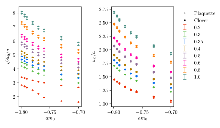
Figure 1: Gradient flow scales $t_{0}$ (left panel) and $w_{0}$ (right panel) as a function of the bare quark mass $am_{0}$, for $\beta=7.2$. Different symbols denote the different definitions of an action density (plaquette or clover). Different colours denote the reference values chosen for $\mathcal{E}_{0}$ and $\mathcal{W}_{0}$. The choices of mass and coupling identify the ensembles from Table 1.

In our previous publication Bennett:2017kga , we performed detailed numerical studies of the GF scheme for the quenched theory, as well as full dynamical calculations for $\beta=6.9$. We found that $w_{0}$ shows smaller cut-off-dependent effects, compared to $t_{0}$. In particular, no significant deviation was found between the values of $w_{0}$ obtained by using the action density at non-zero flow time $E(t)$ constructed from the average plaquette and from the symmetric four-plaquette clover, as defined in Luscher:2010iy .

In this study, we consider a finer lattice with $\beta=7.2$. The results are presented in Fig. 1. We find that while the values of $t_{0}$ show significant discrepancies, the measured values of $w_{0}$ from the two definitions of $E(t)$ are in good agreement over the wide range of $\mathcal{W}_{0}$ and $m_{0}$ we considered, in particular for $\mathcal{W}_{0}=0.3\sim 0.4$. The agreement in the flow scales has improved with respect to the results from coarser lattices in Bennett:2017kga . In Table 1, and in subsequent calculations, we elect to use the gradient flow scale $w_{0}$, which we compute with the reference value of $\mathcal{W}_{0}=0.35$, on the four-plaquette clover action density—for which smaller lattice artefacts are observed. For convenience, we introduce the following notation: $\hat{m}\equiv m^{\rm lat}w_{0}^{\rm lat}=mw_{0}$ denotes the dimensionless quantity corresponding to a mass. We use $\hat{a}\equiv a/w_{0}$ when we discuss lattice-spacing artefacts in Section 4.2.

3.2 Chiral perturbation theory for gradient flow observables

Figure 1 shows that the scales $\sqrt{8t_{0}}/a$ and $w_{0}/a$ depend on the fermion mass $am_{0}$. The title of this subsection is borrowed from Ref. Bar:2013ora , to reflect the fact that we employ the EFT treatment suggested in this reference and we apply it to our numerical results. The EFT treatment assumes that the square root of the flow scale $t_{0}$ is much smaller than the Compton wavelength of the pseudoscalar meson.

Following Bar:2013ora , we use the leading order (LO) relation in the chiral expansion $m_{\rm PS}^{2}=2Bm_{f}$ (where $m_{f}$ is the fermion mass), to write the next-to-leading-order (NLO) result for the GF scale $w_{0}^{\rm NLO}$ as

$$w_{0}^{\rm NLO}(m_{PS}^{2})=w_{0}^{\chi}\left(1+k_{1}\frac{m_{PS}^{2}}{(4\pi f_{\rm PS})^{2}}\right),$$ (11)

where $w_{0}^{\chi}$ is the GF scale and $f_{\rm PS}$ is the pseudoscalar decay constant, both defined in the chiral limit. It is convenient to rescale this expression by writing

$$w_{0}^{\rm NLO}(m_{PS}^{2})/a=(1+\tilde{k}_{1}\hat{m}_{PS}^{2})w_{0}^{\chi}/a,$$ (12)

where $\tilde{k}_{1}$, $w_{0}^{\chi}/a$ and $\hat{m}_{\rm PS}=w_{0}\,m_{\rm PS}$ are dimensionless parameters. We also find it convenient to report here on the extraction of the constants $\tilde{k}_{1}$ and $w_{0}^{\chi}$ from the dynamical ensembles in Table 1. This requires that we anticipate the use of numerical data for the measurement of $m_{\rm PS}/a$ that will be discussed extensively in Section 4 and Appendix A.3, and will be reported in Table 6.

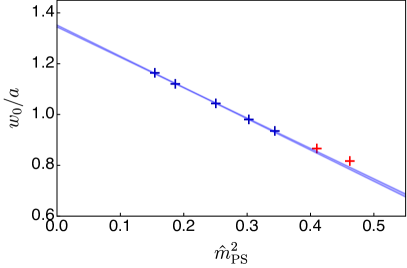
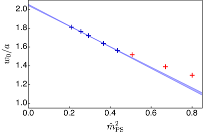
Figure 2: Gradient flow scale dependence on the pseudoscalar meson mass for $\beta=6.9$ (left panel) and $\beta=7.2$ (right panel). Numerical data from Table 1 and from Table 6. The blue bands as based upon Eq. (12), with the fit parameters in Table 2. The band width represents the ($1\sigma$) statistical uncertainties. The fits are restricted to the five ensembles with lightest PS mass (shown in blue), while larger $\hat{m}_{\rm PS}^{2}$ (shown in red) are not included.

$\beta$	$w_{0}^{\chi}/a$	$\tilde{k}_{1}$	$\chi^{2}/N_{\rm d.o.f.}$
$6.9$	$1.347(4)$	$-0.896(12)$	$0.7$
$7.2$	$2.047(8)$	$-0.545(10)$	$0.5$

Table 2: Results of the NLO fits for $w_{0}/a$ from Table 1 and $\hat{m}_{\rm PS}$ from the combination with Table 6. The fit uses the five ensembles with smallest mass to extract the parameters $\tilde{k}_{1}$ and $w_{0}^{\chi}/a$ in Eq. (12).

Figure 2 shows data from Table 1 combined with Table 6, together with the result of the two separate fits (for $\beta=6.9$ and $7.2$) to Eq. (12) of the five ensembles with smallest $\hat{m}_{\rm PS}$. The resulting values of the fit parameters are reported in Table 2. The values of $\chi^{2}/N_{\rm d.o.f.}$ at the minima indicate that chiral perturbation theory for $w_{0}$ well describes the data. Deviations from linear mass dependence of $w_{0}/a$ appear at around $\hat{m}_{\rm PS}^{2}\sim 0.4$. We anticipate that this scale is in broad agreement with the upper bound inferred by studying the pseudoscalar decay constant, and will be discussed in Section 4.

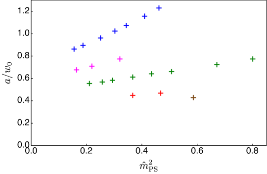
Figure 3: Inverse of the gradient flow scales $w_{0}$ with respect to the pseudoscalar meson mass squared, for data taken from Table 1 and from Table 6. Blue, purple, green, red and brown colours (top to bottom, approximately linear series) have $\beta=6.9$, $7.05$, $7.2$, $7.4$ and $7.5$, respectively.

We observe that the value of $\tilde{k}_{1}$ is smaller for the finer lattice. We have too few ensembles for other lattice couplings to extract the values of $\tilde{k}_{1}$, yet the generic trend is consistent with expectations, as visible in Fig. 3, with the mass-dependence becoming milder for larger choices of $\beta$. Later in the paper, we will perform simultaneous continuum and massless extrapolations via a global fit of all measurements of physical quantities—masses and decay constants of mesons—expressed in units of $w_{0}$.

3.3 Topology

By analogy with the continuum definition ($\frac{1}{32\pi^{2}}\int\mathrm{d}^{4}x\,\varepsilon^{\mu\nu\rho\sigma}\,\mathrm{Tr}\,\left\{F_{\mu\nu}(x){F}^{\rho\sigma}(x)\right\}$), the lattice topological charge of a gauge configuration is defined by summing over lattice sites $i$ as

$$Q\equiv\frac{1}{32\pi^{2}}\sum_{i}\varepsilon^{\mu\nu\rho\sigma}\,\mathrm{Tr}\,\left\{U_{\mu\nu}(i)U_{\rho\sigma}(i)\right\}\;.$$ (13)

The HMC algorithm yields gauge configurations in which ultraviolet fluctuations have typical sizes that are orders of magnitude larger than the desired signal. The resulting large cancellations prevent a reliable extraction of $Q$. A smoothing procedure must be applied, that preserves the topological charge of a configuration while removing UV fluctuations, in order to measure $Q$. The gradient flow described in the earlier subsections can be used for this purpose. For each ensemble, we measure $Q$ from uncorrelated, thermalised configurations, after flowing to a flow time $t/a^{2}={N_{t}^{2}}/32$ (equivalent to $\sqrt{8t}=T/2$).

With our choice of boundary conditions, at finite lattice volume, $Q$ is quantised, and assumes only integer values. Infinitesimal changes in the field configuration cannot alter the topological charge. The change at each Monte Carlo time-step required to yield a good acceptance rate in the Metropolis step of the HMC becomes smaller for fine lattice spacings and small fermion masses. For this reason, at large volumes and small masses, there is a risk that the topological charge freezes at a single value, for the finite HMC trajectories that one implements in practice. Since values of observables may depend on which topological sector is being observed, this effect may introduce a systematic error. To ensure that our measurements are not (heavily) affected by this type of systematic effect, we plot and inspect histories of $Q$ for each ensemble used.

Ensemble	$~{}~{}Q_{0}~{}~{}$	$~{}~{}\sigma~{}~{}$	$~{}~{}\tau_{\exp}~{}~{}$
DB1M1	$0.02(95)$	$8.97(96)$	$\ll 1$
DB1M2	$0.20(85)$	$8.32(85)$	$0.34(23)$
DB1M3	$-0.76(77)$	$8.23(77)$	$\ll 1$
DB1M4	$-0.44(87)$	$8.48(87)$	$\ll 1$
DB1M5	$-0.26(65)$	$6.92(67)$	$0.542(65)$
DB1M6	$1.1(1.7)$	$13.8(1.8)$	$0.36(15)$
DB2M1	$1.28(72)$	$8.06(73)$	$0.82(17)$
DB2M2	$-0.9(1.2)$	$8.9(1.2)$	$0.90(29)$
DB2M3	$-0.7(1.4)$	$12.1(1.4)$	$0.38(20)$
DB3M1	$-0.27(71)$	$6.98(74)$	$1.39(19)$
DB3M2	$-0.50(41)$	$4.61(41)$	$0.90(17)$
DB3M3	$-0.34(48)$	$4.35(48)$	$1.18(25)$
DB3M4	$0.12(89)$	$7.41(93)$	$0.80(17)$
DB3M5	$-0.48(86)$	$7.96(86)$	$1.98(65)$
DB3M6	$-0.45(63)$	$6.24(63)$	$1.21(19)$
DB3M7	$-0.40(60)$	$4.76(60)$	$1.160(81)$
DB3M8	$-0.06(99)$	$8.2(1.0)$	$2.33(32)$
DB4M1	$0.77(60)$	$6.27(60)$	$5.39(28)$
DB4M2	$0.51(93)$	$9.05(94)$	$10.45(18)$
DB5M1	$0.11(24)$	$2.53(24)$	$7.33(36)$

Table 3: Fit results of the topological charge to a Gaussian function for all ensembles. The quantities $Q_{0}$ and $\sigma$ are defined in Eq. (14). They are the mean and the standard deviation for the distribution of the topological charge, respectively. In the last column, we present the results of the exponential autocorrelation time $\tau_{\exp}$ defined in Eq. (16).

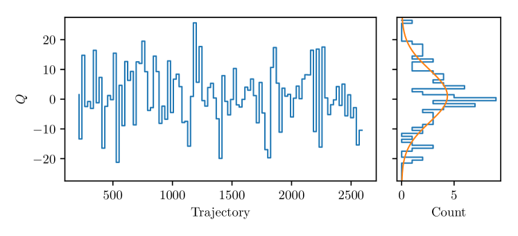
(a) $\beta=6.9,m=-0.85,V=32\times 16^{3}$

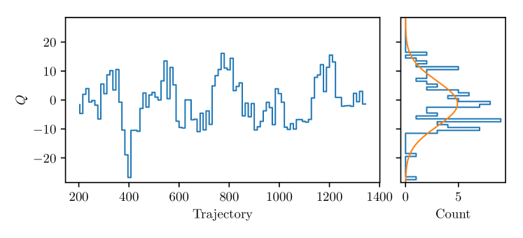
(b) $\beta=7.2,m=-0.78,V=36\times 24^{3}$

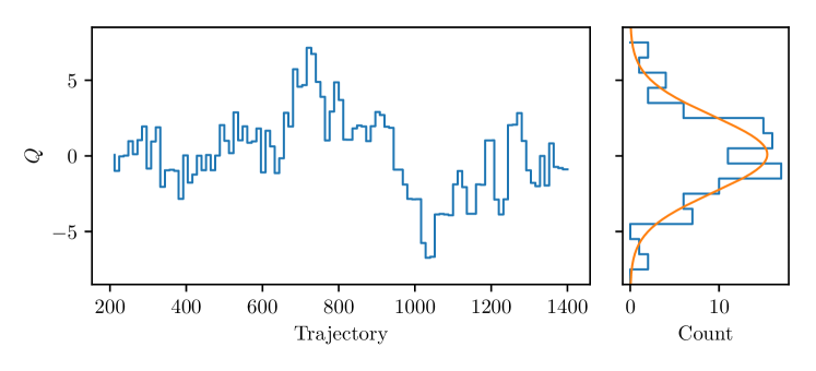
(c) $\beta=7.5,m=-0.69,V=48\times 24^{3}$

Figure 4: Topological charge histories (left), and histograms (right), for the ensembles DB1M1, DB3M5, and DB5M1, respectively. Fitted parameters are (a) $Q_{0}=0.02(95)$, $\sigma=8.97(96)$, $\tau_{\exp}\ll 1$; (b) $Q_{0}=-0.48(86)$, $\sigma=7.96(86)$, $\tau_{\exp}=1.9(7)$; (c) $Q_{0}=0.11(24)$, $\sigma=2.53(24)$, $\tau_{\exp}=7.9(6)$.

We expect the measurements of the charge $Q$ to obey a Gaussian distribution about zero in the limit of infinite simulation time. With a finite number of trajectoris, we use the fitting form

$$n(Q)=A_{n}\exp\left(-\frac{(Q-Q_{0})^{2}}{2\sigma^{2}}\right)$$ (14)

in order to fit the histogram data. The two fit parameters $Q_{0}$ and $\sigma$ are the mean and the standard deviation of the Gaussian distribution. The resulting values are presented in Table 3, while a sample of topological charge histories is shown in Fig. 4.

We also calculate the autocorrelation function $C_{Q}(\tau)$ of the topological charge history as

$$C_{Q}(\tau)=\sum_{\mathfrak{t}=1}^{N-\tau}\frac{(Q_{\mathfrak{t}}-\langle Q\rangle)(Q_{\mathfrak{t}+\tau}-\langle Q\rangle)}{\mathrm{var}(Q)}\;,$$ (15)

where $\mathfrak{t}$ indexes the configurations analysed from 1 to $N$, and $\langle Q\rangle$ and $\mathrm{var}(Q)$ are the mean and variance of $Q$ for these configurations without any assumptions on the distribution. The exponential autocorrelation time $\tau_{\exp}$ is then calculated from this by fitting

$$C_{Q}(\tau)=\exp\left(-\frac{\tau}{\tau_{\exp}}\right)\;.$$ (16)

We report the fit results for $\tau_{\exp}$ in the last column of Table 3. In the ideally decorrelated case, $C_{Q}(\tau)$ is consistent with zero for all $\tau>0$, and so the fit fails to converge; this is checked explicitly, and we report the autocorrelation time as $\tau_{\exp}\ll 1$ in these cases.

All ensembles used to generate the results presented in this paper were found to be free of significant topological freezing, with $Q_{0}$ always within 1$\sigma$ from zero, and the autocorrelation time typically $\tau_{\exp}<2$ and always $\tau_{\exp}\lesssim 10$.

3.4 Finite size effects

The finiteness of the lattice volume represents an inherent source of systematic uncertainties in lattice calculations. In a confining gauge theory, finite-volume (FV) contaminations of the masses and decay constants are expected to be exponentially suppressed as a function of the length of the spatial lattice $L$, at least when the volume is much larger than the inverse of the Compton wavelength of the lightest state, i.e. as long as $m_{\rm PS}L\gg 1$. The size of FV effects can be estimated in a systematic way within chiral perturbation theory, as long as the volume is larger than the hadronic scale. For $f_{\rm PS}L\gtrsim 1$, the dominant contribution is expected to arise from one-loop tadpole integrals of the pseudoscalar mesons Gasser:1986vb ; Golterman:2009kw . The leading-order FV corrections to the meson masses can be written as

$$m_{\rm M}(L)=m_{\rm M}^{\textrm{inf}}\left(1+A_{M}\frac{e^{-m_{\rm PS}^{\rm inf}L}}{(m_{\rm PS}^{\rm inf}L)^{3/2}}\right)\,,$$ (17)

where $m_{\rm M(PS)}^{\rm inf}$ is the meson (pseudoscalar) mass in the infinite volume limit. In principle, the coefficient $A_{M}$ can be determined within chiral perturbation theory without introducing any new parameters in the infinite-volume chiral Lagrangian. Nevertheless, since our data is far from the massless limit, we treat $A_{M}$ as free.

Ensemble	$~{}~{}~{}am_{0}~{}~{}~{}$	$N_{t}\times N_{s}^{3}$	$~{}~{}~{}~{}~{}am_{\rm PS}~{}~{}~{}~{}~{}$	$~{}~{}~{}~{}~{}am_{\rm V}~{}~{}~{}~{}~{}$	$~{}~{}~{}~{}m_{\rm PS}^{\rm inf}\,L~{}~{}~{}~{}$
${\rm DB3M4}^{*}$		$36\times 16^{3}$	0.4267(16)	0.521(4)	6.75
${\rm DB3M4}^{**}$	-0.77	$36\times 20^{3}$	0.4224(12)	0.5153(28)	8.43
DB3M4		$36\times 24^{3}$	0.4222(8)	0.5112(16)	10.12
${\rm DB3M6}^{*}$		$36\times 16^{3}$	0.3309(16)	0.445(4)	5.02
${\rm DB3M6}^{**}$	-0.79	$36\times 20^{3}$	0.3183(10)	0.4290(28)	6.28
DB3M6		$36\times 24^{3}$	0.3153(9)	0.4264(19)	7.53

Table 4: Ensembles and numerical results used to estimate the size of finite volume effects. The number of configurations and the separation of trajectories between adjacent configurations are given by $N_{\rm configs}=200$ and $\delta_{\rm traj}=12$, respectively, for all these ensembles. The pseudoscalar masses in the infinite volume limit $m_{\rm PS}^{\rm inf}$ are estimated from the exponential fits as discussed in the text.

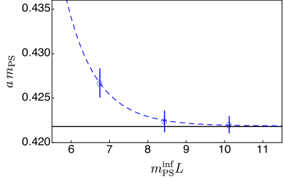
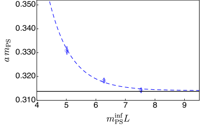
Figure 5: Volume dependence of the pseudoscalar masses, as in Table 4. Lattice parameters are $(\beta,\,m_{0})=(7.2,\,-0.77)$ in the left panel and $(7.2,\,-0.79)$ in the right panel. The (blue) dashed and (black) solid lines denote the fit results and the extrapolated values in the infinite volume limit, respectively.

To quantify the size of FV effects, we calculate masses of pseudoscalar PS and vector V mesons $am_{\rm PS(V)}$ on three spatial lattice volumes of $N_{s}^{3}=16^{3},\,20^{3},\,24^{3}$ at two sets of lattice parameters, $(\beta,\,a\,m_{0})=(7.2,\,-0.77)$ and $(\beta,\,a\,m_{0})=(7.2,\,-0.79)$. Numerical results are reported in Table 4. At the smallest volume $m_{\rm PS}^{\rm inf}\,L\sim 5$, the masses deviate from those at the largest volume by $4\sim 5\%$, more than expected from statistically uncertainties. At $m_{\rm PS}^{\rm inf}\,L\sim 6.3$ the deviations decrease to the level of $1\sim 2\%$, compatible with the statistical uncertainties for $am_{\rm V}$, but not for $am_{\rm PS}$. We performed a fit of the pseudoscalar masses to Eq. (17). As shown in Fig. 5, the data are well described by the exponential fit function: the blue dashed lines correspond to the best fits, while the black solid lines indicate the masses in the infinite volume limit. From this analysis we conclude that the size of FV effects is no larger than $\sim 0.3\%$—smaller than the typical size of statistical uncertainties in the spectroscopic measurements reported in the following sections—if we require that $m_{\rm PS}\,L\gtrsim 7.5$. In the rest of this work we restrict attention to ensembles that satisfy this requirement—see Table 6.

The gradient flow scale also receives a correction from the finite size of the lattice volume. The flow along the fictitious time $t$ can be understood as a smearing procedure with scale $\sqrt{8t}$, hence FV effects are controlled by the dimensionless ratio $c_{\tau}=\sqrt{8t}/L$. At the reference value of $\mathcal{E}_{0}=0.35$ we find that $c_{\tau}$ does not exceed $0.2$ in most ensembles. Using the results in Ref. Fodor:2012td we estimate the size of FV corrections to Eq. (8) to be at most at a few per-mille level. The only exception are the ensembles with $\beta=7.2$ on a $36\times 16^{3}$ lattice and the one with $\beta=7.5$. These ensembles do not play an important role in the analyses that follow, because of the large physical masses associated with them.

4 Meson spectroscopy and decay constants

In this section we summarise the main results of our lattice study, by focusing on the properties (masses and decay constants) of the mesons in the dynamical theory. We start in Section 4.1 by defining the operators we are interested in, the correlation functions we measure, and the renormalisation procedure we apply. We then present all the main spectroscopy results in Section 4.2, and discuss the continuum limit extrapolation in Section 4.3. Useful supplementary details are relegated to Appendix A.2 and A.3.

4.1 Two-point correlation functions

Following established procedure, we extract the masses and the decay constants of flavoured mesons by studying the behaviour of the relevant two-point correlation functions at large Euclidean time $t$. The interpolating operators which carry the same quantum numbers with the desired meson states take the generic form

$$\mathcal{O}_{M}(x)\equiv\overline{Q^{i}}(x)\Gamma_{M}Q^{j}(x),$$ (18)

where $i,j=1,2$ are the flavour indices, and $\Gamma_{M}$ refer to the Dirac structures summarised in Table 5. Summations over spinor and colour indices are understood.

The lightest spin-0 and spin-1 mesons, denoted by PS, V and AV for pseudoscalar, vector and axial-vector mesons, respectively, appear in the low-energy EFT described in Bennett:2017kga . In Section 6 we will use their masses and decay constants to test the EFT and to extrapolate towards the chiral limit. We also consider additional interpolating operators with the Dirac structures $\mathbb{1},\,\gamma^{0}\gamma^{\mu},\,\gamma^{5}\gamma^{0}\gamma^{\mu}$, referred to as scalar S, (antisymmetric) tensor T, and axial tensor AT, though from the related correlation functions we only extract the meson masses. We restrict our attention to the flavoured mesons (by choosing $i\neq j$ in flavour space)— the analogous mesons in QCD are $\pi$, $\rho$, $a_{1}$, $a_{0}$, and $b_{1}$. As the global symmetry is broken, the states created by the interpolating operators denoted by V and T mix, with the low-lying state corresponding to the $\rho$ meson in QCD (see Glozman:2007ek and references therein, as well as Fig. 1 of both Refs. Glozman:2015qva and  Glozman:2018jkb ).

Label ($M$)	Interpolating operator ($\mathcal{O}_{M}$)	Meson	$J^{P}$	$Sp(4)$
PS	$\overline{Q^{i}}\gamma_{5}Q^{j}$	$\pi$	$0^{-}$	$5$
S	$\overline{Q^{i}}Q^{j}$	$a_{0}$	$0^{+}$	$5$
V	$\overline{Q^{i}}\gamma_{\mu}Q^{j}$	$\rho$	$1^{-}$	$10$
T	$\overline{Q^{i}}\gamma_{0}\gamma_{\mu}Q^{j}$	$\rho$	$1^{-}$	$10(+5)$
AV	$\overline{Q^{i}}\gamma_{5}\gamma_{\mu}Q^{j}$	$a_{1}$	$1^{+}$	$5$
AT	$\overline{Q^{i}}\gamma_{5}\gamma_{0}\gamma_{\mu}Q^{j}$	$b_{1}$	$1^{+}$	$10(+5)$

Table 5: Interpolating operators $\mathcal{O}_{M}$ sourcing the lightest mesons in the six channels considered in the main text. To avoid mixing with the flavour singlets, we restrict to $i\neq j$ the flavour indices of the Dirac fermions, while colour and spinor indices are summed and omitted. For completeness, we also show the $J^{P}$ quantum numbers and the corresponding particle in the QCD classification of mesons. Notice that two of the operators source the same particles ($\rho$ meson) because of the breaking of chiral symmetry. In the last column we report the irreducible representation of the unbroken global $Sp(4)$ spanned by the meson (see also Lewis:2011zb ). In brackets are irreducible representations of $Sp(4)$ that are sourced by operators with the same Lorentz structure, but that we do not discuss in this context.

For all the meson interpolating operators $\mathcal{O}_{M}$ listed in Table 5, we define the zero-momentum Euclidean two-point correlation functions at positive Euclidean time $t$ as

$$C_{\mathcal{O}_{M}}(t)\equiv\sum_{\vec{x}}\langle 0|\mathcal{O}_{M}(\vec{x},t)\mathcal{O}_{M}^{\dagger}(\vec{0},0)|0\rangle.$$ (19)

In the numerical study, the resulting mesonic two-point correlation functions are studied by replacing the point-like sources in Eq. (18) with $Z_{2}\times Z_{2}$ single time slice stochastic sources Boyle:2008rh , with number of hits $3$.

Because of the pseudoreal nature of the representation of the symplectic gauge group, diquark operators are indistinguishable from the mesonic operators. We report in Table 5 also the multiplicity of each state (the size of the irreducible representation of $Sp(4)$). For instance, five pNGBs form a multiplet of the unbroken $Sp(4)$, in the $SU(4)\rightarrow Sp(4)$ enhanced symmetry pattern of the gauge theory considered here. Compared with what happens with gauge group $SU(N)$, these five pNGBs include the three associated with the breaking $SU(2)_{L}\times SU(2)_{R}\rightarrow SU(2)_{V}$, together with two diquarks. In Appendix A.2 we explicitly show the equivalence of meson and diquark correlators by using the lattice action in Eq. (4).

At large Euclidean time $t$ the correlation functions in Eq. (19) are dominated by the lowest excitation at zero spatial momentum so that the mass $m_{M}$ appears in the asymptotic expression:

$$C_{\mathcal{O}_{M}}(t)\xrightarrow{t\rightarrow\infty}\langle 0|\mathcal{O}_{M}|M\rangle\langle 0|\mathcal{O}_{M}|M\rangle^{*}\frac{1}{2m_{M}}\left[e^{-m_{M}t}+e^{-m_{M}(T-t)}\right]\,,$$ (20)

where $T$ is the temporal extent of the lattice. The decay constants $f_{M}$ are determined from the matrix elements, which are parameterised as

$$\langle 0|\overline{Q_{1}}\gamma_{5}\gamma_{\mu}Q_{2}|{\rm PS}\rangle = f_{\rm PS}p_{\mu}\,,$$

$$\langle 0|\overline{Q_{1}}\gamma_{\mu}Q_{2}|{\rm V}\rangle = f_{\rm V}m_{\rm V}\epsilon_{\mu}\,,$$

$$\langle 0|\overline{Q_{1}}\gamma_{5}\gamma_{\mu}Q_{2}|{\rm AV}\rangle = f_{\rm AV}m_{\rm AV}\epsilon_{\mu}\,.$$ (21)

The polarisation vector $\epsilon_{\mu}$ is transverse to the momentum $p_{\mu}$ and normalised by $\epsilon_{\mu}^{*}\epsilon^{\mu}=1$. The meson states $|M\rangle$ are conventionally defined by the self-adjoint isospin fields, as in $M=M^{A}T^{A}$, where $T^{A}$ are the generators of the group. We adopt conventions such that in QCD the analogous experimental value of the pion (pseudoscalar) decay constant is $f_{\pi}\simeq 93\,{\rm MeV}$. In Eq. (21), the pseudoscalar decay constant $f_{\rm PS}$ is defined via the local axial current. To calculate the decay constant $f_{PS}$, we introduce an additional two-point correlation function

$$C_{\Pi}(t) = \sum_{\vec{x}}\langle 0|[\overline{Q_{1}}\gamma_{5}\gamma_{\mu}Q_{2}(\vec{x},t)]\,[\overline{Q_{1}}\gamma_{5}Q_{2}(\vec{0},0)]|0\rangle$$ (22)

$$\xrightarrow{t\rightarrow\infty} \frac{f_{\rm PS}\langle 0|\mathcal{O}_{\rm PS}|{\rm PS}\rangle^{*}}{2}\left[e^{-m_{\rm PS}t}-e^{-m_{\rm PS}(T-t)}\right],$$

where $\langle 0|\mathcal{O}_{\rm PS}|{\rm PS}\rangle^{*}$ can be obtained from $C_{\mathcal{O}_{\rm PS}}(t)$ in Eq. (20). In practice, we calculate $m_{\rm PS}$ and $f_{\rm PS}$ by performing a simultaneous fit to the numerical data for $C_{\mathcal{O}_{\rm PS}}(t)$ and $C_{\Pi}(t)$. The details of the fit of the meson correlators, including the effective masses and best-fit ranges, are provided in Appendix A.3.

The matrix elements in Eq. (21), calculated from the lattice at finite lattice spacing $a$, must be converted to those renormalised in the continuum. For Wilson fermions the decay constants in the continuum are determined from lattice ones via

$$f_{\rm PS}=Z_{\rm A}f^{\rm bare}_{\rm PS},~{}~{}~{}f_{\rm V}=Z_{\rm V}f_{\rm V}^{\rm bare},~{}~{}~{}{\rm and}~{}~{}~{}f_{\rm AV}=Z_{\rm A}f_{\rm AV}^{\rm bare},$$ (23)

where $Z_{\rm V}$ and $Z_{\rm A}$ are the renormalisation factors for vector and axial-vector currents which are expected to approach unity in the continuum. Since the pseudoscalar decay constant $f_{\rm PS}$ is defined using the axial current as in Eq. (21), it receives renormalisation with the factor of $Z_{\rm A}$. The renormalisation factors are determined by the one-loop renormalisation procedure in lattice perturbation theory for Wilson fermions, and the expressions for the matching factors are the following Martinelli:1982mw :

$$Z_{A} = 1+C(F)\left(\Delta_{\Sigma_{1}}+\Delta_{\gamma_{5}\gamma_{\mu}}\right)\frac{\tilde{g}^{2}}{16\pi^{2}},$$

$$Z_{V} = 1+C(F)\left(\Delta_{\Sigma_{1}}+\Delta_{\gamma_{\mu}}\right)\frac{\tilde{g}^{2}}{16\pi^{2}}.$$ (24)

The eigenvalue of the quadratic Casimir operator with fundamental fermions is $C(F)=5/4$ for the $Sp(4)$ gauge theory. The one-loop factor $\Delta_{\Sigma_{1}}$ arises from the wave-function renormalisation of the external fermion lines, while the other $\Delta$’s arise from the one-loop computations of the vertex functions. The numerical values obtained by one-loop integrals within the continuum $\overline{\rm MS}$ (modified minimal subtraction) renormalisation scheme are as follows: $\Delta_{\Sigma_{1}}=-12.82$, $\Delta_{\gamma_{\mu}}=-7.75$ and $\Delta_{\gamma_{5}\gamma_{\mu}}=-3.0$. The coupling used in Eq. (24) is defined via the mean field approach to the link variable, which effectively removes the tadpole diagrams, as $\tilde{g}^{2}=g^{2}/\langle P\rangle$ Lepage:1992xa , where $\langle P\rangle$ is the average plaquette value and $g$ the bare gauge coupling.

4.2 Masses and decay constants

Ensemble	$am_{\rm PS}$	$af_{\rm PS}$	$am_{\rm S}$	$m_{\rm PS}\,L$	$f_{\rm PS}\,L$
DB1M1	0.8344(11)	0.1431(7)	1.52(4)	13.351(17)	2.290(10)
DB1M2	0.7403(12)	0.1299(11)	1.44(4)	11.845(19)	2.079(17)
DB1M3	0.6276(14)	0.1147(8)	1.15(5)	10.042(23)	1.836(13)
DB1M4	0.5625(21)	0.1052(11)	1.290(20)	9.00(3)	1.683(18)
DB1M5	0.4813(10)	0.0943(6)	1.04(5)	7.701(16)	1.509(10)
DB1M6	0.3867(11)	0.0823(6)	1.032(25)	9.28(26)	1.977(13)
DB1M7	0.3388(12)	0.0765(6)	0.92(5)	8.13(3)	1.835(14)
DB2M1	0.4376(14)	0.0822(9)	0.88(3)	8.752(28)	1.645(17)
DB2M2	0.3311(11)	0.0670(5)	0.830(16)	7.946(26)	1.609(13)
DB2M3	0.2729(9)	0.0612(4)	0.777(13)	8.732(27)	1.958(12)
DB3M1	0.6902(11)	0.0994(9)	1.046(25)	11.043(18)	1.590(14)
DB3M2	0.5898(13)	0.0905(8)	0.994(16)	9.437(21)	1.449(13)
DB3M3	0.4700(13)	0.0772(6)	0.838(13)	7.521(21)	1.235(10)
DB3M4	0.4222(8)	0.0726(3)	0.792(11)	10.133(18)	1.743(8)
DB3M5	0.3702(9)	0.0666(4)	0.744(13)	8.884(21)	1.598(9)
DB3M6	0.3153(9)	0.0604(4)	0.646(18)	7.568(22)	1.448(9)
DB3M7	0.2874(7)	0.05755(28)	0.665(12)	8.048(19)	1.611(8)
DB3M8	0.2532(7)	0.0536(3)	0.598(17)	8.102(24)	1.714(10)
DB4M1	0.3190(5)	0.05452(23)	0.576(9)	10.208(15)	1.745(7)
DB4M2	0.2707(6)	0.04999(27)	0.548(8)	8.663(20)	1.600(9)
DB5M1	0.3264(9)	0.0529(4)	0.562(7)	7.835(23)	1.270(9)

Table 6: Masses and (renormalised) decay constants for flavoured mesons sourced by pseudoscalar (PS) and scalar (S) operators in units of the lattice spacing $a$. The pseudoscalar decay constant $f_{PS}$ is renormalised via the one-loop perturbative matching in Eq. (23). Statistical uncertainties are indicated in parenthesis.

Ensemble	$am_{\rm V}$	$af_{\rm V}$	$am_{\rm AV}$	$af_{\rm AV}$	$am_{\rm T}$	$am_{\rm AT}$
DB1M1	0.9275(17)	0.2326(15)	1.561(29)	0.228(14)	0.9277(21)	1.512(24)
DB1M2	0.8475(19)	0.2224(14)	1.445(26)	0.215(11)	0.8475(27)	1.434(29)
DB1M3	0.7494(25)	0.2056(18)	1.315(24)	0.211(10)	0.754(3)	1.276(25)
DB1M4	0.692(4)	0.1917(25)	1.27(3)	0.217(14)	0.688(5)	1.205(29)
DB1M5	0.622(3)	0.1777(21)	1.16(4)	0.191(21)	0.619(4)	1.169(21)
DB1M6	0.546(4)	0.1629(20)	1.059(14)	0.193(5)	0.547(5)	0.97(3)
DB1M7	0.517(4)	0.1564(23)	0.97(4)	0.163(14)	0.527(6)	0.96(4)
DB2M1	0.5517(24)	0.1445(14)	0.918(28)	0.139(10)	0.554(4)	0.933(26)
DB2M2	0.470(3)	0.1284(20)	0.825(23)	0.135(8)	0.466(5)	0.834(24)
DB2M3	0.4237(29)	0.1202(14)	0.75(3)	0.120(11)	0.424(5)	0.736(27)
DB3M1	0.7490(17)	0.1478(16)	1.142(16)	0.146(6)	0.7484(23)	1.154(9)
DB3M2	0.6591(25)	0.1408(14)	1.036(15)	0.146(6)	0.659(3)	1.038(13)
DB3M3	0.5529(26)	0.1269(15)	0.879(18)	0.127(7)	0.555(3)	0.905(14)
DB3M4	0.5112(16)	0.1208(10)	0.847(13)	0.129(5)	0.5138(16)	0.788(16)
DB3M5	0.4664(25)	0.1121(15)	0.789(14)	0.125(5)	0.4750(28)	0.785(21)
DB3M6	0.4264(19)	0.1083(9)	0.720(20)	0.114(8)	0.426(3)	0.696(24)
DB3M7	0.4019(23)	0.1040(11)	0.698(10)	0.116(3)	0.4013(27)	0.715(13)
DB3M8	0.3772(24)	0.0990(13)	0.650(15)	0.107(5)	0.386(3)	0.643(17)
DB4M1	0.3974(11)	0.0905(6)	0.623(11)	0.092(5)	0.3976(15)	0.635(9)
DB4M2	0.3548(17)	0.0844(9)	0.560(8)	0.0853(27)	0.3528(21)	0.555(11)
DB5M1	0.3941(20)	0.0832(12)	0.594(8)	0.0851(26)	0.391(3)	0.596(11)

Table 7: Masses and (renormalised) decay constants for flavoured mesons sourced by vector (V), axial-vector (AV), and tensor (T) and axial-tensor (AT) operators in lattice units. The V and AV decay constants are renormalised via the one-loop perturbative matching in Eq. (23). Statistical uncertainties are indicated in parenthesis.

Figure 6: Top panel: pseudoscalar masses squared $\hat{m}_{\rm PS}$ and decay constants squared $\hat{f}^{2}_{\rm PS}$ as a function of the subtracted bare fermion mass. Green and blue symbols stand for $\hat{m}_{\rm PS}^{2}$ and $\hat{f}_{\rm PS}^{2}$, respectively. Bottom panel: left-hand side of the GMOR relation, as a function of the subtracted fermion mass. All points computed with $\beta=7.2$. The uncertainty on the horizontal axis descends form the determination of $\hat{m}_{0}^{c}$.

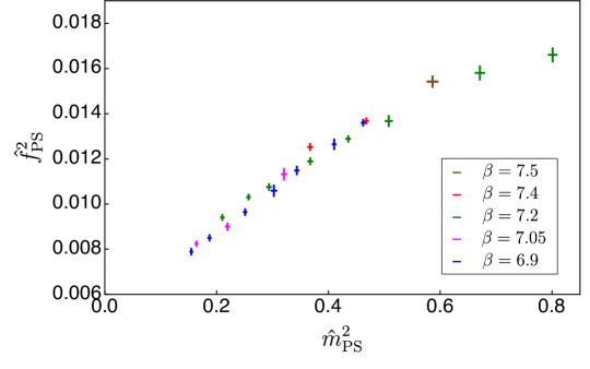
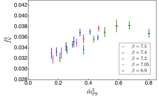
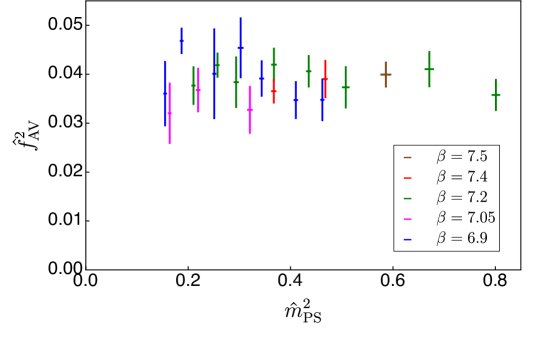
Figure 7: Decay constant squared for pseudoscalar (PS, top), vector (V, middle) and axial-vector (AV, bottom) mesons as a function of the pseudoscalar mass squared $\hat{m}_{\rm PS}^{2}$. Different colours refer to different lattice couplings as shown in the legends. The error bars represent the size of statistical uncertainties. (See Appendix A.3 for the details.)

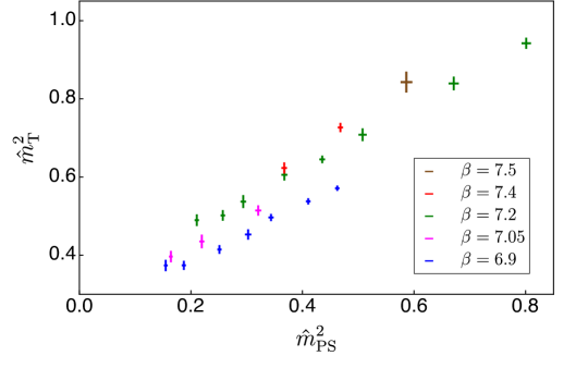
Figure 8: Mass squared of mesons sourced by vector (V, top) and tensor (T, bottom) operators as a function of the pseudoscalar mass squared $\hat{m}_{\rm PS}^{2}$. Different colours refer to different lattice couplings as shown in the legends. The error bars represent the size of statistical uncertainties. (See Appendix A.3 for the details.)

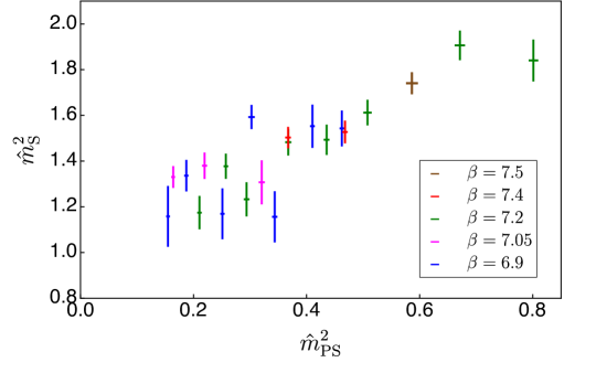
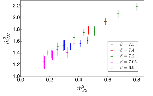
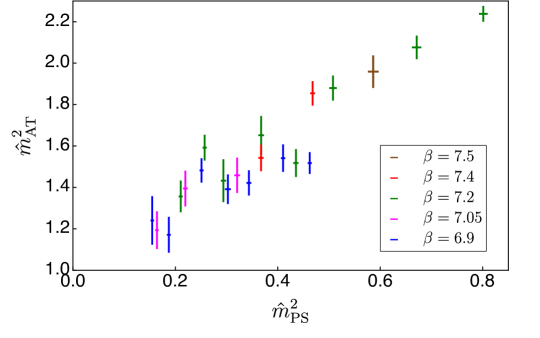
Figure 9: Mass squared of mesons sourced by scalar (S, top), axial-vector (AV, middle) and axial-tensor (AT, bottom) operators as a function of the pseudoscalar mass squared $\hat{m}_{\rm PS}^{2}$. Different colours refer to different lattice couplings as shown in the legends. The error bars represent the size of statistical uncertainties. (See Appendix A.3 for the details.)

Using the techniques described in the previous subsection, we calculate meson masses and decay constants for the ensembles in Table 1. The resulting values in lattice units are summarised in Table 6 for mesons sourced by PS and S operators, and in Table 7 for those sourced by V, AV, T, and AT operators. The decay constants in the tables are renormalised as in Eq. (23). As expected, the pseudoscalar mesons are the lightest states for all ensembles. In Table 6 we also present the numerical values of $m_{\rm PS}L$ and $f_{\rm PS}L$. The lattice volumes in all ensembles are large enough that $m_{\rm PS}L\gtrsim 7.5$, and, as we discussed in Section 3.4, finite volume effects are negligible. Furthermore, all the values of $f_{\rm PS}$ satisfy the condition $f_{\rm PS}L>1$, to ensure that the lattice volume is large enough to capture the chiral symmetry breaking scale. The ensembles to be used for the massless and continuum extrapolations are further restricted to $f_{\rm PS}L\gtrsim 1.5$.

Mesons with higher mass (and spin) can in principle decay into 2 and/or 3 pseudoscalars Drach:2017btk , but for all the ensembles we considered they cannot decay due to large pseudoscalar masses. Table 7 shows that the masses of mesons sourced by V and T operators are in good agreement, within current statistical uncertainties. As is the case within QCD, low-lying states identified by a given set of quantum numbers $(I,J^{PC})$ can result from admixture of more than one possible operator when the global symmetry is strongly broken Glozman:2007ek . We also find that the masses of three heavier states, sourced by S, AV, and AT operators, and that have different quantum numbers, are close to one another. They are affected by large statistical and systematical uncertainties when their masses are extracted from the two-point correlation functions (see Appendix A.3 for technical details).

In order to compare to one another results obtained from ensembles at different bare parameters, we must relate them to the corresponding renormalised quantities in the continuum limit. We do so by adopting the GF scheme as explained in Section 3.1: we define the meson masses and decay constants in units of $w_{0}$ using the notation

$$\hat{m}_{M}\equiv m_{M}w_{0}=m^{\rm lat}_{M}w_{0}^{\rm lat}~{}{\rm and}~{}\hat{f}_{M}\equiv f_{M}w_{0}=f^{\rm lat}_{M}w_{0}^{\rm lat}.$$ (25)

We can compare measurements at different lattice couplings $\beta$, and use the EFT to remove residual artefacts due to the discretisation. This procedure will be explained in detail in section 4.3.

On the lattice, the bare fermion mass $m_{f}$ is a free parameter. It can vary from being very small (yielding very light pseudoscalars) to assuming somewhat large values (yielding stable vector mesons). A detailed study of the renormalisation of the fermion mass $m_{f}$ requires a dedicated study that goes beyond the purposes of this work. In its stead, we replaced $m_{f}$ by the pseudoscalar mass squared $m_{\rm PS}^{2}$, which is a physical quantity. In the low-energy EFT, the two are related through the LO relation $m_{\rm PS}^{2}=2Bm_{f}$, with $B$ one of the coefficients in the chiral Lagrangian.

Before proceeding, we must check what is the regime of parameters for which the LO mass relation between fermion mass and pseudoscalar mass is a good approximation to the data. To illustrate this point, in the top panel of Fig. 6 we present the pseudoscalar masses squared $\hat{m}_{\rm PS}^{2}$ and decay constants squared $\hat{f}_{\rm PS}^{2}$ against the bare mass—after subtracting the effects of lattice additive renormalisation $(\hat{m}_{0}-\hat{m}_{0}^{c})$—for ensembles at $\beta=7.2$, with various bare masses. The critical mass $\hat{m}_{0}^{c}$ is determined numerically, extrapolating from the linear fit to the lightest five data points to the value for which $\hat{m}_{\rm PS}^{2}=0$. As shown in the figure, deviation from linearity appear for $\hat{m}_{\rm PS}^{2}>0.4$. The decay constant squared also shows a linear behaviour, and its slope is not negligible. The bottom panel of Fig. 6 shows deviations from linearity of the dependence of the combination $m_{\rm PS}^{2}f_{\rm PS}^{2}$ on the fermion mass. The Gell-Mann-Oakes-Renner (GMOR) relation GellMann:1968rz , $m_{\rm PS}^{2}f_{\rm PS}^{2}=m_{f}\langle\bar{\psi}\psi\rangle$, would imply a mass dependence of the fermion condensate over the range of mass considered. We alert the reader that a rigorous discussion of the GMOR relation would require first to determine the values of $\hat{m}_{0}^{c}$ for each fixed choice of $\hat{a}$ (obtained by adjusting both the bare mass and coupling, while keeping the lattice spacing in units of $w_{0}$ fixed), while in this simplified discussion we kept the lattice coupling $\beta=7.2$ fixed. This is adequate for the purposes of this subsection, but we refer the reader to Section 6.1 for an assessment of the validity of the GMOR relation in the continuum limit.

In Fig. 7 we show the numerical results of the decay constants squared of PS, V and AV mesons, while in Figs. 8 and 9 we present the masses squared of mesons sourced by the operators V and T, and by S, AV, and AT, respectively, as functions of $\hat{m}_{\rm PS}^{2}$. Our first observation is that discretisation effects in $\hat{f}_{\rm PS}^{2}$ and $\hat{m}_{\rm V}^{2}$ (or $\hat{m}_{\rm T}^{2}$) are significant, given the visible difference between data collected at different lattice couplings (and denoted by different colours). For other quantities the deviations are no larger than the statistical uncertainties. Also, the masses and the decay constants decrease as we approach the massless limit, with the exception of $\hat{f}_{\rm AV}^{2}$. Overall, the masses and decay constants show linear dependence on $\hat{m}_{\rm PS}^{2}$ in a wide range inside the small-mass region.

4.3 Continuum extrapolation

We are now in a position to perform the continuum extrapolation, and to eliminate discretisation artefacts in the meson masses and decay constants. In order to do so, we introduce the important tool of W$\chi$PT Sheikholeslami:1985ij ; Rupak:2002sm (see also Ref. Sharpe:1998xm , and Symanzik:1983dc ; Luscher:1996sc ). It extends the continuum effective field theory by a double expansion, both in small fermion mass $m$, as well as lattice spacing $a$, as both of them break chiral symmetry and can be introduced in the EFT as spurions. We denote the lattice spacing in units of $w_{0}$ by

$$\hat{a}\equiv a/w_{0}=1/w_{0}^{\rm lat}.$$ (26)

This yields the natural size of discretisation effects, consistently with the fact that we measure all other dimensional quantities in units of $w_{0}$.

At NLO in W$\chi$PT Rupak:2002sm , the tree-level expression for the pseudoscalar decay constant leads to

$$\hat{f}_{\rm PS}^{\rm NLO}=\hat{f}^{\chi}\left(1+\hat{b}_{f}^{\chi}\hat{m}_{\rm PS}^{2}\right)+\hat{W}_{f}^{\chi}\hat{a},$$ (27)

where $\hat{f}^{\chi}=f^{\chi}w_{0}^{\chi}$ is the pseudoscalar decay constant in the massless and continuum limit. The fermion masses used in this study are comparatively large, and hence it is legitimate to omit from Eq. (27) the chiral logs, which are important for small values of $\hat{m}_{\rm PS}$. The coefficients $\hat{b}_{f}^{\chi}$ and $\hat{W}_{f}^{\chi}$ control the size of corrections due to finite mass and finite lattice spacing, respectively. In principle one should measure all observables in units of $w_{0}^{\chi}$, while we instead use the mass-dependent $w_{0}$, as measured at the finite mass of the individual ensembles, hence avoiding the need to extrapolate to the massless limit Ayyar:2017qdf —we collected enough data to attempt such extrapolation only for two values of $\beta$. The replacement of $w_{0}^{\chi}$ by $w_{0}$ does not affect the NLO EFT, the difference appearing at higher orders in $m_{\rm PS}^{2}$. Compared to the continuum NLO expression in Ref. Bijnens:2009qm , it results in a shift $\hat{b}_{f}^{\chi}$ by $\tilde{k}_{1}$ in Eq. (12), due to fitting the measurements of $f_{\rm PS}w_{0}$.

	$~{}~{}\hat{f}^{2,\,\chi}_{M}~{}~{}$	$~{}~{}~{}L^{0}_{f,M}~{}~{}~{}$	$~{}~{}~{}~{}~{}W^{0}_{f,M}~{}~{}~{}~{}~{}$	$~{}~{}~{}~{}~{}\chi^{2}/N_{\rm d.o.f}~{}~{}~{}~{}~{}$
PS	$0.00618(28)(33)$	$3.01(21)(33)$	$-0.00135(29)(19)$	$1.6$
V	$0.0296(15)(8)$	$0.51(9)(6)$	$0.0004(16)(8)$	$1.0$
AV	$0.032(7)(2)$	$0.17(35)(14)$	$0.012(8)(2)$	$1.1$
	$~{}~{}\hat{m}^{2,\,\chi}_{M}~{}~{}$	$~{}~{}~{}L^{0}_{m,M}~{}~{}~{}$	$~{}~{}~{}~{}~{}W^{0}_{m,M}~{}~{}~{}~{}~{}$	$~{}~{}~{}~{}~{}\chi^{2}/N_{\rm d.o.f}~{}~{}~{}~{}~{}$
V	$0.404(13)(9)$	$2.18(10)(7)$	$-0.220(15)(12)$	$0.9$
T	$0.418(18)(2)$	$2.08(12)(17)$	$-0.229(22)(30)$	$0.8$
AV	$1.07(13)(2)$	$1.37(32)(7)$	$0.04(13)(2)$	$0.8$
AT	$1.08(13)(8)$	$1.49(34)(16)$	$-0.08(13)(13)$	$2.4$
S	$1.16(12)(12)$	$0.85(21)(20)$	$-0.08(14)(16)$	$1.8$

Table 8: Fit results of the continuum and massless extrapolations for masses squared and decay constants squared of mesons in the dynamical simulations. The low-energy constants appearing in W$\chi$PT are defined in Eqs. (30) and (31). The fits of $\hat{f}_{\rm PS}^{2}$ measurements are restricted to include only the eleven ensembles identified in the main text. For the other quantities, additional ensembles satisfying $\hat{m}_{\rm PS}^{2}\mathrel{\raisebox{-2.32501pt}{$\stackrel{{\scriptstyle\textstyle<}}{{\sim}}$}}0.6$ and $\hat{a}\mathrel{\raisebox{-2.32501pt}{$\stackrel{{\scriptstyle\textstyle<}}{{\sim}}$}}1$ have been included. In parenthesis, we report the statistical and systematic uncertainties, respectively.

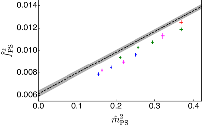
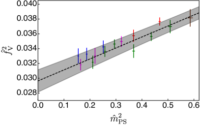
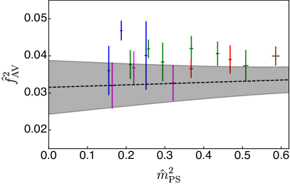
Figure 10: Top to bottom, left to right: decay constants squared of the pseudoscalar (PS), vector (V), and axial-vector (AV) mesons, as a function of the pseudoscalar mass squared $\hat{m}_{\rm PS}^{2}$. Various colours denote different lattice couplings: $\beta=6.9$ (blue), $7.05$ (purple), $7.2$ (green), $7.4$ (red), and $7.5$ (brown). The grey bands (the width of which indicates the statistical error) show the results of the continuum and massless extrapolations after subtracting the discretisation artefact, as discussed in the text.

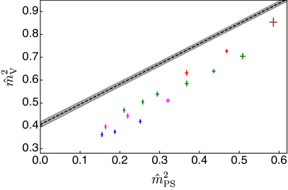
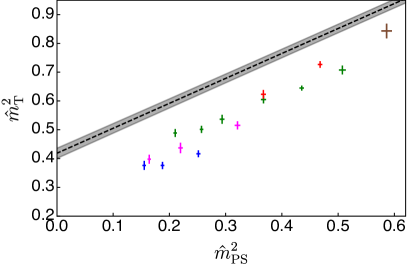
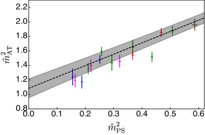
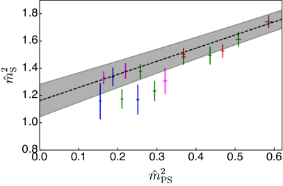
Figure 11: Top to bottom, left to right: masses squared of the vector (V), tensor (T), axial-vector (AV), axial-tensor (AT), and scalar (S) mesons, as a function of the pseudoscalar mass squared $\hat{m}_{\rm PS}^{2}$. Various colours denote different lattice couplings: $\beta=6.9$ (blue), $7.05$ (purple), $7.2$ (green), $7.4$ (red), and $7.5$ (brown). The grey bands (the width of which indicates the statistical error) show the results of the continuum and massless extrapolations after subtracting the discretisation artefact, as discussed in the text.

Among the underlying assumptions of W$\chi$PT is the requirement that the measurements it describes satisfy

$$\frac{m_{\rm PS}^{2}}{\Lambda_{\chi}^{2}}\sim a\Lambda_{\chi}<1,$$ (28)

where $\Lambda_{\chi}$ is the symmetry breaking scale, for which we take the estimate $\Lambda_{\chi}=4\pi f_{\rm PS}$. In Section 3.2, we found the NLO EFT to describe the measurements of $\hat{w}_{0}$ up to $\hat{m}_{\rm PS}^{2}\mathrel{\raisebox{-2.58334pt}{$\stackrel{{\scriptstyle\textstyle<}}{{\sim}}$}}0.4$. The numerical results for the pseudoscalar decay constant squared in Fig. 7 shows linear mass dependence over the range of $0.15\mathrel{\raisebox{-2.58334pt}{$\stackrel{{\scriptstyle\textstyle<}}{{\sim}}$}}\hat{m}_{\rm PS}^{2}\mathrel{\raisebox{-2.58334pt}{$\stackrel{{\scriptstyle\textstyle<}}{{\sim}}$}}0.40$. Using the (bare) results in Table 1, restricted to this range, the two mass scales associated with the power counting for the tree-level NLO W$\chi$PT are estimated to be

$$0.13\mathrel{\raisebox{-2.58334pt}{$\stackrel{{\scriptstyle\textstyle<}}{{\sim}}$}}\frac{m_{\rm PS}^{2}}{\Lambda_{\chi}^{2}}\sim 0.20\,,~{}~{}~{}{\rm and}~{}~{}~{}0.60\mathrel{\raisebox{-2.58334pt}{$\stackrel{{\scriptstyle\textstyle<}}{{\sim}}$}}a\Lambda_{\chi}\sim 1.4.$$ (29)

The first estimate is roughly consistent with the scale separation in Eq. (28). But we find that $a\Lambda_{\chi}$ evaluated on some of the ensembles is greater than unity. We further constrain the analysis to the ensembles that satisfy the condition $\hat{a}\lesssim 1$, which is satisfied by DB1M5$-$7, DB2M1$-$3, DB3M5$-$8, and DB4M2. Only these ensembles will be used in the continuum and massless extrapolations that employ the tree-level NLO W$\chi$PT. We will report the values of the $\chi^{2}/N_{\rm d.o.f.}$ in the analysis, and we anticipate here that the quality of the fits of the data supports the results of this exclusion process, otherwise based upon a set of estimates.

As the linear dependence of $\hat{f}_{\rm PS}^{\rm NLO}$ on both $\hat{m}_{\rm PS}^{2}$ and $\hat{a}$ can be recast into linear behaviour of $\hat{f}_{\rm PS}^{2,{\rm NLO}}$ and because—on the basis of the EFT described in Bennett:2017kga —at NLO also the mass squared and decay constant squared of spin-1 mesons have leading corrections of $\mathcal{O}(m_{\rm PS}^{2})$, we consider the following linear ansatz:

$$\hat{f}_{M}^{2,{\rm NLO}} = \hat{f}_{M}^{2,\chi}\left(1+L_{f,M}^{0}\hat{m}_{\rm PS}^{2}\right)+W_{f,M}^{0}\hat{a}$$ (30)

for the decay constants squared of the mesons $M=$ PS, V, and AV, and

$$\hat{m}_{M}^{2,{\rm NLO}} = \hat{m}_{M}^{2,\chi}\left(1+L_{m,M}^{0}\hat{m}_{\rm PS}^{2}\right)+W_{m,M}^{0}\hat{a}$$ (31)

for the masses squared of the mesons $M=$ V, AV, S, T, and AT.

We restrict the fit to the eleven ensembles identified earlier for $\hat{f}_{\rm PS}^{2}$. Yet, the results for V, AV, S, T and AT mesons in Figs. 7, 8 and 9 exhibit linear dependence on $\hat{m}_{\rm PS}^{2}$ also in heavier ensembles, so that in the fits of their properties we included additional ensembles with $\hat{m}_{\rm PS}^{2}\sim 0.6$ and $\hat{a}\lesssim 1$. The fit results are presented in Figs. 10 and 11. In the figures, the grey bands denote the continuum extrapolated results obtained by setting $\hat{a}=0$ in Eqs. (30) and (31), and by using the fit parameters summarised in Table 8. In the table, the numbers in the two parentheses denote the statistical and systematic uncertainties associated with the numerical fits. The latter is estimated by varying the fitting range to include or exclude the coarsest or the heaviest ensemble. We find acceptable values of $\chi^{2}/{\rm d.o.f}$ for all the fits, in support of the applicability of the tree-level NLO EFT to describe our data.

5 Lattice results: summary

We provide here a list of lattice highlights (from Sections 2, 3, and 4). We will be very schematic: precise definitions and detailed discussions can be found in the main text.

• The lattice ensembles used in the dynamical study, and the values of the lattice parameters that characterise them, are discussed in Section 2, and listed in Table 1, including the average plaquette and the gradient flow scale $w_{0}$.

• The gradient flow scale $w_{0}$ is defined and studied in Section 3.1. Its mass dependence is illustrated by Fig. 1, 2, and 3 and Table 2. Throughout this work we employ the gradient flow scale to set the physical scale of the lattice calculations.

• The topological charge is defined and studied in Sec. 3.3, and examples of topological charge histories are depicted in Fig. 4. The ensembles used in the numerical analysis do not show clear evidence of topological freezing.

• Lattice finite size effects are studied in Section 3.4. They are negligibly small provided the condition $m_{\rm PS}L\mathrel{\raisebox{-2.58334pt}{$\stackrel{{\scriptstyle\textstyle>}}{{\sim}}$}}7.5$ is satisfied—see also Table 4 and Fig. 5. In the analysis presented in this paper, all ensembles satisfy this condition.

• In Section 4, we define the operators and the two-point functions used for the measurement of decay constants and masses of the mesons—see Table 5. The decay constants are perturbatively renormalised according to Eqs. (23) and (24).

• The masses and (renormalised) decay constants (in units of the lattice spacing $a$) of the spin-0 mesons are reported in Table 6, and those of the spin-1 mesons in Table 7.

• In Sec. 4.2 we introduce the notation $\hat{m}\equiv m_{M}w_{0}$, and equivalent for all dimensional quantities expressed in terms of the gradient flow scale. We discuss the GMOR relation and illustrate it in Figure 6. Linearity with the fermion mass holds for $\hat{m}_{\rm PS}^{2}\mathrel{\raisebox{-2.58334pt}{$\stackrel{{\scriptstyle\textstyle<}}{{\sim}}$}}0.4$. From this point on, we eliminate the dependence on the fermion mass, and study our observables only as a function of the mass (squared) of the PS state.

• Masses and decay constants, expressed in units of the gradient flow scale, are plotted for all ensembles in Figs. 7, 8, and 9. We notice that the V and T masses are compatible with each other, and so are the AV and AT—although the latter two states are physically distinct. We do not further discuss the T and AT states in the paper.

• We apply tree-level W$\chi$PT via Eqs. (30) and (31), that we use to perform the continuum and massless extrapolations. We impose the conditions $\hat{a}\mathrel{\raisebox{-2.58334pt}{$\stackrel{{\scriptstyle\textstyle<}}{{\sim}}$}}1$, $m_{\rm PS}L\mathrel{\raisebox{-2.58334pt}{$\stackrel{{\scriptstyle\textstyle>}}{{\sim}}$}}7.5$, and $m_{\rm PS}^{2}\mathrel{\raisebox{-2.58334pt}{$\stackrel{{\scriptstyle\textstyle<}}{{\sim}}$}}0.4$, which identify a subset of eleven ensembles to be used for the continuum extrapolation of $\hat{f}_{\rm PS}^{2}$. For the other observables we relax the condition on the mass to $m_{\rm PS}^{2}\mathrel{\raisebox{-2.58334pt}{$\stackrel{{\scriptstyle\textstyle<}}{{\sim}}$}}0.6$. The results are shown in Table 8 and in Figs. 10 and 11.

• As reflected in the fit results for $W^{0}$ presented in Table 8, $\hat{f}_{\rm PS}^{2}$ and $\hat{m}_{\rm V}^{2}$ (and similarly $\hat{m}_{\rm T}^{2}$) are affected by discretisation effects, the sizes of which are about $4\sim 13\%$ and $10\sim 35\%$, respectively, over the considered ranges of bare parameters. In all other observables, discretisation effects are no larger than the statistical errors.

6 Low-energy phenomenology: EFT and sum rules

In this section, we study some of the long distance properties of the $Sp(4)$ gauge theory that may be useful inputs for phenomenological studies performed in the context of composite Higgs models based upon the $SU(4)/Sp(4)$ coset. We restrict our attention to the PS, V and AV states, and consider only ensembles with $\hat{a}\mathrel{\raisebox{-2.58334pt}{$\stackrel{{\scriptstyle\textstyle<}}{{\sim}}$}}1$ and $\hat{m}_{\rm PS}^{2}\mathrel{\raisebox{-2.58334pt}{$\stackrel{{\scriptstyle\textstyle<}}{{\sim}}$}}0.4$. We perform a simplified continuum extrapolation, by subtracting from their masses and decay constants the last term of Eqs. (30) and (31), with the coefficients $W^{0}_{f,M}$ and $W^{0}_{m,M}$ obtained by a fit similar to the one presented in Sec. 4.3, but restricted to include only the eleven ensembles that satisfy all the constraints. We then use the resulting eleven independent measurements of the three masses and three decay constants, that we report in Table 9, to perform a simplified global fit based upon the NLO EFT in Ref. Bennett:2017kga . The results of the fit allow us to provide an extrapolation to the massless limit, and to assess the validity of the EFT itself by providing a first estimate of the size of the $g_{VPP}$ coupling between a vector state V and two pseudoscalar states PS. We also discuss several phenomenological quantities of general interest, connected with classical current algebra results, such as the aforementioned GMOR relation GellMann:1968rz , and the saturation of the Weinberg sum rules Weinberg:1967kj by the lightest spin-1 states.

Ensemble	$10~{}\hat{a}~{}$	$10~{}\hat{m}_{\rm PS}^{2}~{}$	$100~{}\hat{f}^{2}_{\rm PS}~{}$	$10~{}\hat{m}_{\rm V}^{2}~{}$	$100~{}\hat{f}^{2}_{\rm V}~{}$	$~{}~{}\hat{m}_{\rm AV}^{2}~{}~{}$	$100~{}\hat{f}^{2}_{\rm AV}$
DB1M5	9.603(17)	2.512(22)	1.092(21)	6.19(13)	3.24(14)	1.44(16)	2.8(11)
DB1M6	8.932(11)	1.873(19)	0.969(23)	5.59(12)	3.15(14)	1.38(13)	3.5(8)
DB1M7	8.607(9)	1.549(17)	0.903(25)	5.40(13)	3.13(17)	1.24(17)	2.5(10)
DB2M1	7.728(12)	3.20(3)	1.230(30)	6.71(15)	3.35(13)	1.39(13)	2.3(7)
DB2M2	7.068(11)	2.192(26)	0.993(23)	5.90(17)	3.17(16)	1.35(15)	2.8(8)
DB2M3	6.740(6)	1.637(17)	0.914(23)	5.36(15)	3.05(15)	1.23(17)	2.3(10)
DB3M5	6.109(11)	3.68(3)	1.270(21)	7.09(17)	3.25(13)	1.65(10)	3.4(6)
DB3M6	5.820(11)	2.94(3)	1.153(22)	6.57(16)	3.35(13)	1.51(14)	3.1(8)
DB3M7	5.669(6)	2.574(21)	1.106(20)	6.20(16)	3.25(14)	1.50(12)	3.5(7)
DB3M8	5.522(7)	2.105(21)	1.014(21)	5.81(17)	3.11(15)	1.37(14)	3.1(8)
DB4M2	4.466(7)	3.67(3)	1.312(20)	7.24(14)	3.49(12)	1.56(10)	3.1(5)

Table 9: Input data used in the continuum EFT global fit. We consider only ensembles with $\hat{a}\mathrel{\raisebox{-2.32501pt}{$\stackrel{{\scriptstyle\textstyle<}}{{\sim}}$}}1$ and $\hat{m}_{\rm PS}^{2}\mathrel{\raisebox{-2.32501pt}{$\stackrel{{\scriptstyle\textstyle<}}{{\sim}}$}}0.4$. For each ensemble, we subtracted the finite lattice spacing effect, according to Eqs. (30) and (31), with the coefficients $W^{0}_{f,M}$ and $W^{0}_{m,M}$ obtained by a fit restricted to these ensembles.

6.1 Global fit and low-energy constants

The EFT presented in Ref. Bennett:2017kga describes the low-energy behaviour of the lightest PS, V, and AV mesons, by adopting the ideas of HLS Bando:1984ej ; Casalbuoni:1985kq ; Bando:1987br ; Casalbuoni:1988xm ; Harada:2003jx . The extension of the chiral Lagrangian is achieved by enhancing the $SU(4)$ global symmetry to $SU(4)_{A}\times SU(4)_{B}$, weakly gauging the $SU(4)_{A}$ group factor, and implementing the spontaneous breaking to the global $Sp(4)$ by the VEVs of two spin-0 fields subject to non-linear constraints, and transforming one on the bi-fundamental of $SU(4)_{A}\times SU(4)_{B}$ and the other on the antisymmetric of $SU(4)_{A}$, respectively. In this way, besides the $5$ pNGBs identified with the PS states of the theory, the spectrum also contains $15$ massive spin-1 particles, identified with the $10$ V and $5$ AV states. Explicit breaking of the global symmetry due to the fermion mass $m_{f}$ is implemented by the familiar spurion analysis. The results for physical quantities in terms of the $12$ free parameters ($f$, $F$, $b$, $c$, $g_{V}$, $\kappa$, $v$, $v_{1}$, $v_{2}$, $v_{5}$, $y_{3}$, $y_{4}$) of the EFT are summarised in Eqs. (2.19)-(2.24), together with Eqs. (2.29), (2.30) and (2.33) of Ref. Bennett:2017kga .

The simplified global fit in Ref. Bennett:2017kga suffered from uncontrolled systematics such as quenching effects and discretisation artefacts. In this paper, we overcome these limitations with the continuum extrapolations of the data obtained by dynamical simulations, as discussed in previous sections. A further technical difficulty of the global fit is due to the large parameter space and the limited number of observables available. Because we employ Wilson fermions, we have one more unknown fit parameter, the critical bare fermion mass $m_{0}^{c}$, if we use the bare mass $m_{0}$ for the fermion mass in the EFT. A better way to determine the parameters in the EFT might be to consider a more sophisticated definition of the fermion mass, such as the one calculated via partially conserved axial current (PCAC). However, this would require to carry out a more involved computation of the renomalisation factors associated with the pseudoscalar operators, which is beyond the scope of this work.

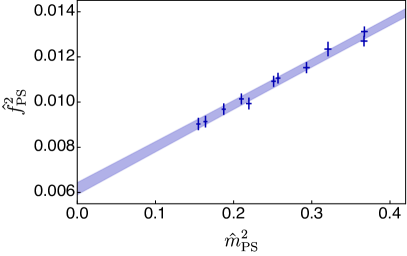
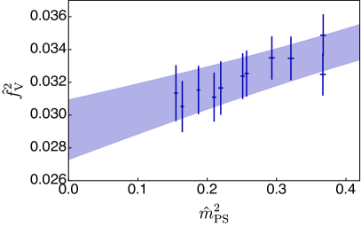
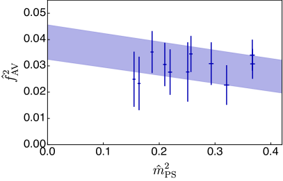
Figure 12: Decay constants squared in the continuum limit—subtracting lattice artefacts due to a finite lattice spacing (see Table 9)—as a function of the pseudoscalar mass $\hat{m}_{\rm PS}^{2}$. The bars represent the statistical uncertainties. The global fit results are denoted by shaded bands whose widths indicate the statistical errors.

Along the lines discussed in Section 4.2, here we take a different approach. We eliminate from the analysis any direct reference to the fermion mass, effectively replacing its role with the mass of the PS state. Because the linear relation $m_{\rm PS}^{2}=2Bm_{f}$ holds only at leading-order, we restrict our attention to ensembles for which $\hat{m}_{\rm PS}^{2}\lesssim 0.4$ (see Table 9). Furthermore, we expand the dependence of the other observable masses and decay constants Bennett:2017kga on $\hat{m}_{\rm PS}^{2}$, truncating at linear order. (We express all quantities in units of $w_{0}$.) Up to $\mathcal{O}(\hat{m}_{\rm PS}^{4})$, we find

$$\hat{m}_{\rm V}^{2} = \frac{g_{\rm V}^{2}(b\hat{f}^{2}+\hat{F}^{2})}{4(1+\kappa)}+\frac{2\hat{v}_{1}(\kappa+1)-\hat{y}_{3}(b\hat{f}^{2}+\hat{F}^{2})}{4(\kappa+1)^{2}}g_{\rm V}^{2}\hat{m}_{\rm PS}^{2},$$ (32)

$$\hat{m}_{\rm AV}^{2} = \frac{(b+4)\hat{f}^{2}+\hat{F}^{2}}{4(1-\kappa)}g_{\rm V}^{2}+\frac{\left((b+4)\hat{f}^{2}+\hat{F}^{2}\right)\hat{y}_{4}-2(1-\kappa)(\hat{v}_{1}-2\hat{v}_{2})}{4(1-\kappa)^{2}}g_{\rm V}^{2}\hat{m}_{\rm PS}^{2},$$ (33)

$$\hat{f}_{\rm V}^{2} = \frac{1}{2}(b\hat{f}^{2}+\hat{F}^{2})+\hat{v}_{1}\hat{m}_{\rm PS}^{2},$$ (34)

$$\hat{f}_{\rm AV}^{2} = \frac{(\hat{F}^{2}-b\hat{f}^{2})^{2}}{2((b+4)\hat{f}^{2}+\hat{F}^{2})}-\frac{((3b+8)\hat{v}_{1}-4(b+2)\hat{v}_{2})\hat{f}^{2}+\hat{F}^{2}\hat{v}_{1}}{((b+4)\hat{f}^{2}+\hat{F}^{2})^{2}}(\hat{F}^{2}-b\hat{f}^{2})\hat{m}_{\rm PS}^{2},$$ (35)

$$\hat{f}_{\rm PS}^{2} = \frac{2\hat{f}^{2}((b+4c+bc)\hat{f}^{2}+(1+b+c)\hat{F}^{2})}{(4+b)\hat{f}^{2}+\hat{F}^{2}}+$$

$$-\frac{4(2+b)\hat{f}^{2}((2+b)\hat{f}^{2}\hat{v}_{1}+(\hat{F}^{2}-b\hat{f}^{2})\hat{v}_{2})}{((4+b)\hat{f}^{2}+\hat{F}^{2})^{2}}\hat{m}_{\rm PS}^{2}\,,$$

having make use of the redefinitions

$$\hat{f}\equiv fw_{0},~{}\hat{F}\equiv Fw_{0},~{}\hat{y}_{3}\equiv\frac{y_{3}}{2\hat{B}w_{0}},~{}\hat{y}_{4}\equiv\frac{y_{4}}{2\hat{B}w_{0}},~{}\hat{v}_{1}\equiv\frac{v_{1}w_{0}}{2\hat{B}},~{}\hat{v}_{2}\equiv\frac{v_{2}w_{0}}{2\hat{B}},$$ (37)

and

$$\hat{B}\equiv Bw_{0}\,,~{}~{}~{}~{}~{}~{}~{}~{}B\equiv v^{3}/(2f_{\rm PS}^{2})\,.$$ (38)

This linearised ansatz involves $10$ unknown parameters ($\hat{f}$, $\hat{F}$, ${b}$, ${c}$, ${g}_{V}$, ${\kappa}$, $\hat{v}_{1}$, $\hat{v}_{2}$, $\hat{y}_{3}$, $\hat{y}_{4}$) to be determined from $5$ measurements. The remaining two parameters ($v$ and $v_{5}$) are associated with the GMOR relation, as they enter at NLO the definition of $\hat{m}_{\rm PS}^{2}$. We will return to this point later on.

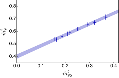
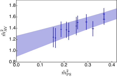
Figure 13: Masses squared in the continuum limit—subtracting lattice artefacts due to a finite lattice spacing (see Table 9)—as a function of the pseudoscalar mass $\hat{m}_{\rm PS}^{2}$. The bars represent the statistical uncertainties. The global fit results are denoted by shaded bands whose widths indicate the statistical errors.

We perform a global fit using the functions in Eqs. (32)-(6.1). The $\chi^{2}$ function is defined in a simplified manner, by summing the individual $\chi^{2}$ obtained from the five independent fit equations, and hence ignoring correlations among the fit equations. Besides subtracting the discretisation effects $W^{0}_{m,M}\hat{a}$ and $W^{0}_{f,M}\hat{a}$ from the original data, and restricting consideration to $\hat{m}_{\rm PS}^{2}\lesssim 0.4$ and $\hat{a}\lesssim 1$, as anticipated, we also constrain the fit by implementing the following conditions, which are the consequences of unitarity Bennett:2017kga :

$$1 > \kappa+\hat{m}_{\rm PS}^{2}\hat{y}_{4},$$

$$-1 < \kappa+\hat{m}_{\rm PS}^{2}\hat{y}_{3},$$

$$0 < b\hat{f}^{2}+\hat{F}^{2}+2\hat{m}_{\rm PS}^{2}\hat{v}_{1},$$

$$0 < 2+b+c+(b+4c)\frac{\hat{f}^{2}}{\hat{F}^{2}}-2\hat{m}_{\rm PS}^{2}\hat{v}_{1},$$ (39)

$$0 < b\left((c+1)\hat{f}^{2}+\hat{F}^{2}-2\hat{m}_{\rm PS}^{2}\hat{v_{1}}+2\hat{m}_{\rm PS}^{2}\hat{v}_{2}\right)+$$

$$+c\left(4\hat{f}^{2}+\hat{F}^{2}-2\hat{m}_{\rm PS}^{2}\hat{v_{1}}+4\hat{m}_{\rm PS}^{2}\hat{v}_{2}\right)-\frac{\hat{m}_{\rm PS}^{4}\hat{v}_{2}^{2}}{\hat{f}^{2}}+\hat{F}^{2}-2\hat{m}_{\rm PS}^{2}\hat{v}_{1}.$$

	$~{}~{}\hat{f}^{2,\,\chi}_{M}~{}~{}$	$~{}~{}~{}L^{0}_{f,M}~{}~{}~{}$	$~{}~{}\hat{m}^{2,\,\chi}_{M}~{}~{}$	$~{}~{}~{}L^{0}_{m,M}~{}~{}~{}$
PS	$0.00617(28)(36)$	$3.02(22)(35)$
V	$0.0291(18)(11)$	$0.45(16)(14)$	$0.400(16)(10)$	$2.16(15)(9)$
AV	$0.039(7)(2)$	$-0.82(15)(8)$	$1.07(19)(8)$	$1.42(6)(3)$

Table 10: Coefficients appearing in Eqs. (30) and (31), determined by using the results of the global fit described in the main text. The results are compatible with those obtained with the alternative fit process in Table 8, except for the coefficient $L^{0}_{f,{\rm AV}}$.

In Figs. 12 and 13 we present the continuum values of the masses and decay constants from Table 9, along with the results of the global fits, represented by blue bands, obtained through a constrained bootstrapped $\chi^{2}$ minimisation with 10 parameters, with the constraints guided by an initial minimisation of the full data set. The fit functions describe the data well, with $\chi^{2}/N_{\rm d.o.f}\sim 0.4$. But we also find that some of the EFT parameters are not well determined (see discussion in Appendix B, in particular the histograms of $200$ resampled data obtained by bootstrapping, for the LO parameters in Fig. 21 and for the NLO ones in Fig. 22), indicating the presence of flat directions in the $\chi^{2}$.

The fact that the EFT yields a good quality fit of the masses and decay constants justifies using its results to calculate other physical quantities. The coupling $g_{\rm VPP}$ is responsible for the decay of the vector meson into two pseudoscalar mesons. The NLO EFT expression can be found in Bennett:2017kga (where $g_{\rho\pi\pi}$ denotes $g_{\rm VPP}$) and in the massless limit we have that the $g_{\rm VPP}^{\chi}$ coupling is

$$g_{\rm VPP}^{\chi}=\frac{g_{\rm V}(b+2)(2\hat{f}^{2}+\hat{F}^{2})(b\hat{f}^{2}+\hat{F}^{2})}{((b+4)\hat{f}^{2}+\hat{F}^{2})((b+(b+4)c)\hat{f}^{2}+(b+c+1)\hat{F}^{2})\sqrt{1+\kappa}}\,.$$ (40)

We find that $g_{\rm VPP}^{\chi}=6.0(4)(2)$—see also Appendix B, in particular the histogram of the coupling in Fig. 23, which shows a nice gaussian distribution.

As a consistency check, we also calculate the relevant coefficients in Eqs. (30) and (31), by using the results of the global fit. We present the results in Table 10: they are consistent with the ones in Table 8, with the only exception of $L^{0}_{f,{\rm AV}}$ which is over-constrained by Eqs. (32)-(6.1), but also affected by larger systematic as well as statistical uncertainties.

The results of this exercise have to be taken with caution, for a number of reasons. The fermion masses considered are not small enough to fully justify the linearisation of the fit equations, nor the truncation of the EFT itself to exclude higher-order terms. This is also clear from the fact that the masses considered are such that the V mesons are stable, because the 2-PS channel is closed. These objections can be addressed in the future, by lowering the fermion mass studied on the lattice. Also, the coupling $g_{\rm V}$ (or alternatively the coupling $g_{\rm VPP}$) turns out not to be small, bring into question the truncation of the EFT. This coupling should be suppressed if we consider future lattice studies of $Sp(2N)$ theories with $N\geq 3$.

6.2 GMOR relation and Weinberg sum rules

There are several consequences of the HLS EFT (and of current algebra) that can be tested on our lattice data. If we first restrict our attention to the PS sector, we have the GMOR relation, which at NLO takes the corrected form

$$m_{\rm PS}^{2}f_{\rm PS}^{2}=m_{f}(v^{3}+m_{f}v_{5}^{2}),$$ (41)

where $v$ and $v_{5}$ are the two low-energy constants defined in Ref. Bennett:2017kga that we removed from our global fit. As noted in Section 4.2, we cannot extract $v$ and $v_{5}$ without renormalisation of the fermion mass. In Fig. 14 we plot the numerical results of $\hat{m}_{\rm PS}^{2}\hat{f}_{\rm PS}^{2}$ with respect to $\hat{m}_{\rm PS}^{2}$, as an illustration of Eq. (41).

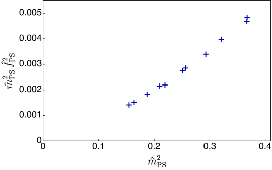
Figure 14: The quantity $\hat{m}_{\rm PS}^{2}\hat{f}_{\rm PS}^{2}$ entering the GMOR relation, for the data set of $\hat{m}_{\rm PS}^{2}\lesssim 0.4$ and $\hat{a}\lesssim 1$, in the continuum limit (see Table 9).

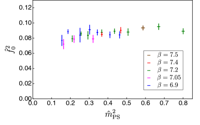
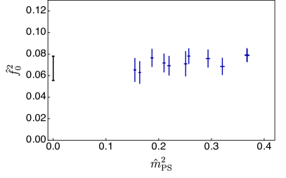
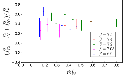
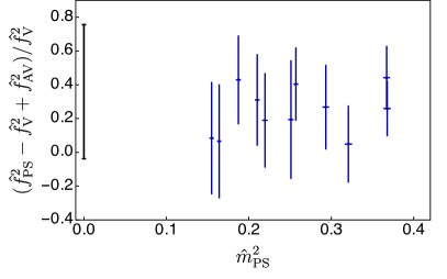
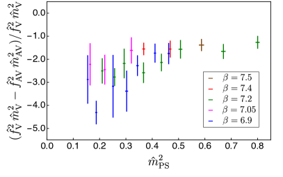
Figure 15: Top to bottom: $\hat{f}_{0}^{2}$, the first, and the second Weinberg sum rule, saturated over the lightest spin-1 states, as a function of $\hat{m}_{\rm PS}^{2}$. Left panels: we do not perform the continuum extrapolation, colour coding represents the bare lattice coupling of the various ensembles. Blue, purple, green, red and brown colours have $\beta=6.9$, $7.05$, $7.2$, $7.4$ and $7.5$, respectively. Right panels: continuum-extrapolation results as in Table 9 (in blue), and the results of the continuum and massless extrapolation (in black). Statistical and systematic errors are summed in quadrature.

Going beyond the pseudoscalar sector, the first non-trivial prediction of the NLO EFT—related to some reasonable assumptions for the truncation of the series of operators—is that the sum of the decay constants (at zero momentum)

$$f_{0}^{2} \equiv f_{\rm PS}^{2}+f_{\rm V}^{2}+f_{\rm AV}^{2}\,,$$ (42)

is expected to be independent on the fermion mass. In the top-left panel of Fig. 15 we plot the numerical results of $\hat{f}_{0}^{2}$ with respect to $\hat{m}_{\rm PS}^{2}$, with the continuum extrapolation shown in the top-right panel. As seen in the figure, at the level of the present precision the numerical results support the mass independence of $f_{0}^{2}$ over the range of mass considered.

While the Weinberg spectral theorems, which involve integration over all momenta, are exact, because they reflect the properties of the underlying condensates in the theory Weinberg:1967kj , the saturation of the resulting sum rules over a finite number among the lightest spin-1 states is an approximation. The NLO EFT analysis captures such violations in the non-nearest-neighbour interactions appearing in the HLS Lagrangian. These terms are generated by integrating out heavier resonant spin-1 states that contribute to the dispersion relations. Saturated over the lightest resonances, the first and second sum rules are

$$f_{\rm AV}^{2}-f_{\rm V}^{2}+f_{\rm PS}^{2} = 0\,,$$ (43)

and

$$f_{\rm V}^{2}m_{\rm V}^{2}-f_{\rm AV}^{2}m_{\rm AV}^{2} = 0\,,$$ (44)

respectively. The aforementioned corrections give finite contributions to the right-hand-side of these two relations. The numerical results for these quantities, normalised by $f_{\rm V}^{2}$ and $f_{\rm V}^{2}m_{\rm V}^{2}$, respectively, are shown in the middle and bottom panels of Fig. 15. As the figures show, after continuum extrapolation the results are closer to saturating the Weinberg sum rules. The conservative estimate of the uncertainties includes both statistical and systematic error, and with its current size this comparison is somewhat inconclusive.

7 Comparison to other gauge theories

Ensemble	$\hat{m}_{\rm V}/\hat{m}_{\rm PS}$	$\hat{m}_{\rm PS}/\hat{f}_{\rm PS}$	$\hat{m}_{\rm V}/\hat{f}_{\rm PS}$	$\hat{m}_{\rm AV}/\hat{f}_{\rm PS}$	$\hat{m}_{\rm S}/\hat{f}_{\rm PS}$	$\hat{f}_{\rm V}/\hat{f}_{\rm PS}$	$\hat{f}_{\rm AV}/\hat{f}_{\rm PS}$
DB1M5	1.569(18)	4.80(5)	7.53(13)	11.5(6)	10.9(6)	1.72(4)	1.6(3)
DB1M6	1.728(20)	4.40(6)	7.60(14)	11.9(6)	12.3(6)	1.80(4)	1.90(21)
DB1M7	1.867(26)	4.14(6)	7.74(15)	11.7(8)	11.9(9)	1.86(5)	1.6(4)
DB2M1	1.446(18)	5.10(6)	7.37(13)	10.6(5)	10.7(5)	1.65(3)	1.34(23)
DB2M2	1.640(26)	4.70(6)	7.71(16)	11.6(7)	12.2(5)	1.78(5)	1.65(26)
DB2M3	1.807(28)	4.24(5)	7.66(16)	11.6(8)	12.5(6)	1.83(5)	1.6(4)
DB3M5	1.390(17)	5.38(5)	7.47(12)	11.4(4)	11.1(4)	1.60(3)	1.63(14)
DB3M6	1.497(19)	5.05(5)	7.55(13)	11.4(5)	10.7(5)	1.70(3)	1.62(21)
DB3M7	1.553(21)	4.82(5)	7.49(13)	11.6(5)	11.5(5)	1.72(4)	1.76(17)
DB3M8	1.662(25)	4.55(5)	7.57(15)	11.6(6)	11.1(6)	1.75(4)	1.72(23)
DB4M2	1.403(15)	5.29(4)	7.43(10)	10.9(3)	10.9(4)	1.63(3)	1.53(14)
Massless	N/A	N/A	8.08(32)	13.4(1.5)	14.2(1.7)	2.15(8)	2.3(4)

Table 11: Ratios of meson masses and decay constants, extrapolated to the continuum limit by the subtraction method explained in Section 4.3. We restrict the data to the eleven ensembles for which the subtraction of effects due to the finite lattice spacing can be done for all measurable quantities. In the last row, we report the results of the continuum and massless extrapolation, obtained by applying Eqs. (30) and (31) to the eleven ensembles. Statistical and systematic uncertainties have been added in quadrature.

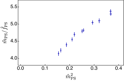
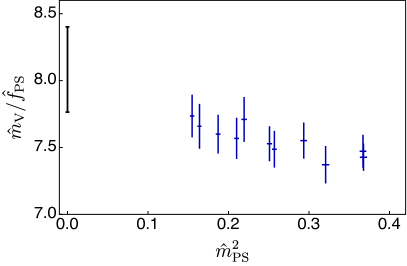
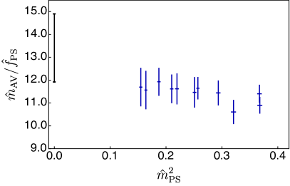
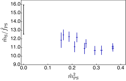
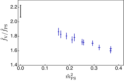
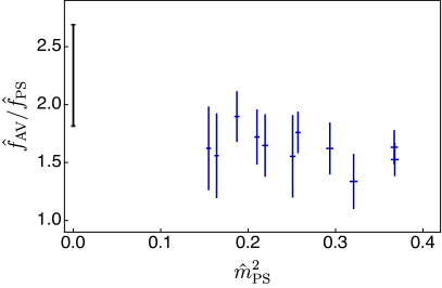
Figure 16: Ratios of masses and decay constants, in the continuum limit, expressed in units of the decay constant of the PS meson (as in Table 11), shown in blue. We also show the extrapolation to the continuum and massless limit in black, except for $\hat{m}_{\rm PS}$, which vanishes in the limit of massless fermions.

This section is devoted to comparing our results with those obtained in a few other lattice gauge theories with two Dirac fermions. We start by presenting our results in a different way, by normalising all masses and decay constants to the decay constant $f_{\rm PS}$ of the lightest PS state. By doing so, we remove direct reference to the gradient flow scale $w_{0}$, and make the comparison to other theories more transparent. We report the results of this exercise in Table 11 and Fig. 16. We restrict attention to the eleven ensembles for which we are able to take the continuum limit for all the observables, as described in Section 4.3. We then compare our results to those obtained in gauge theories with $SU(2)$ Arthur:2016dir , $SU(3)$ Jansen:2009hr , and $SU(4)$ Ayyar:2017qdf with matter field content consisting of $N_{f}=2$ Dirac fermions in the fundamental. We do so by testing the validity of the two phenomenological Kawarabayashi-Suzuki-Riazuddin-Fayyazuddin (KSRF) relations Kawarabayashi:1966kd ; Riazuddin:1966sw . We conclude this section with a comparison to the continuum extrapolation of the quenched $Sp(4)$ theory; details of additional quenched computations performed beyond those presented in Ref. Bennett:2017kga to facilitate this analysis are presented elsewhere Sp4ASFQ .

The fermion masses in the selected eleven ensembles are moderately heavy, with $1.39\mathrel{\raisebox{-2.58334pt}{$\stackrel{{\scriptstyle\textstyle<}}{{\sim}}$}}\hat{m}_{\rm V}/\hat{m}_{\rm PS}\mathrel{\raisebox{-2.58334pt}{$\stackrel{{\scriptstyle\textstyle<}}{{\sim}}$}}1.87$, so that both V and AV mesons are stable, as the decay channels to two and three PS mesons, respectively, are kinematically forbidden. Bearing this in mind, we nevertheless apply Eqs. (30) and (31) to the eleven ensembles, and we perform the massless (and continuum) extrapolations. In the last row of the Table 11 we report the resulting ratios of the masses and decay constants to $\hat{f}_{\rm PS}$, which are rendered in black colour in Figure 16 . Notice that the ratio are independent of the gradient flow scale $w_{0}$, so that $f_{\rm V}/f_{\rm PS}=\hat{f}_{\rm V}/\hat{f}_{\rm PS}$ (and analogous for all dimensionless quantities in Table 11).

The spectroscopy of the lightest meson states is captured to some approximation by the two KSRF phenomenological relations Kawarabayashi:1966kd ; Riazuddin:1966sw . The first such relation states that

$$f_{\rm V}=\sqrt{2}f_{\rm PS}\,,$$ (45)

which is rather close to real-world QCD, as taking the experimental value of the rho meson decay constant to be $f_{\rho}\simeq 148$ MeV, yields $f_{\rho}/f_{\pi}\sim 1.6$ Tanabashi:2018oca . We can compare our results for $Sp(4)$ with the first KSRF relation by looking at $\hat{f}_{\rm V}/\hat{f}_{\rm PS}$ in Figure 16. For $\hat{m}_{\rm PS}^{2}<0.4$ the ratio monotonically increases from $\hat{f}_{\rm V}/\hat{f}_{\rm PS}\sim 1.5$ as $\hat{m}_{\rm PS}^{2}$ decreases. A simple linear extrapolation yields the ratio in the massless and continuum limit to be $\hat{f}_{\rm V}/\hat{f}_{\rm PS}\sim 2.1$. Therefore, our numerical results do not support the first KSRF relation: the resulting values not only depend on the fermion mass, but also become larger in the massless limit.

The second KSRF relation involves $m_{\rm V}$, $f_{\rm PS}$, and the on-shell coupling constant $g_{\rm VPP}$ associated with the decay of a vector meson:

$$g_{\rm VPP}=\frac{m_{\rm V}}{\sqrt{2}f_{\rm PS}}.$$ (46)

In real-world QCD, the mass of $\rho$ meson $m_{\rho}\simeq 775$ MeV, expressed in units of the pion decay constant $f_{\pi}$, yields roughly $m_{\rho}/\sqrt{2}f_{\pi}\sim 5.9$ Tanabashi:2018oca . For comparison, we adopt the tree-level definition for the decay rate of $\rho$ meson, $\Gamma_{\rho}=\frac{g_{\rho\pi\pi}^{2}}{48\pi}m_{\rho}\left(1-\frac{4m_{\pi}^{2}}{m_{\rho}^{2}}\right)^{3/2}$, and the reference experimental values $\Gamma_{\rho}\simeq 150$ MeV and $m_{\pi}\simeq 140$ MeV. We find $g_{\rho\pi\pi}\simeq 6.0$, which is in quite good agreement. By evaluating the right-hand side of the second KSRF relation for the $Sp(4)$ gauge theory, computed with the lightest ensemble and in the massless limit, we find ${\hat{m}_{\rm V}}/{\sqrt{2}\hat{f}_{\rm PS}}=5.47(11)$ and ${\hat{m}_{\rm V}}/{\sqrt{2}\hat{f}_{\rm PS}}=5.72(18)(13)$, respectively. By comparing with the independent measurement of $g_{\rm VPP}=6.0(4)(2)$ from Section 6, obtained from the global fit of the EFT, we conclude that the second KSRF relation holds.

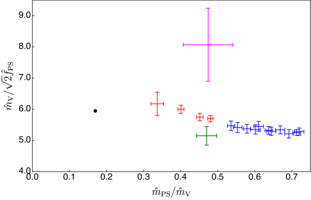
Figure 17: The ratios of the vector mass and pseudoscalar decay constant $m_{\rm V}/\sqrt{2}f_{\rm PS}$ in several lattice gauge theories with $N_{f}=2$ fundamental Dirac flavours. Purple, red, green and blue colours are for $SU(2)$ Arthur:2016dir , $SU(3)$ Jansen:2009hr , $SU(4)$ Ayyar:2017qdf and $Sp(4)$ gauge groups, respectively. The $Sp(4)$ result obtained in this work are obtained in the continuum limit for the eleven ensembles identified in Section 4.3. The black circle is the experimental value of the coupling in the real world of QCD. Notice that for the $SU(2)$ and $SU(4)$ theories we show only the lightest data points, extracted approximately from the plots in the respective publications.

It is interesting to compare the right-hand side of the second KSRF relation with other lattice results available in the literature on $SU(N)$ gauge theories with two fundamental Dirac fermions. We show the comparison in Fig. 17. For the lightest ensembles available, it is found that in the continuum limit $m_{\rm V}/\sqrt{2}f_{\rm PS}\sim 8.1(1.2)$ for $SU(2)$ Arthur:2016dir and $m_{\rm V}/\sqrt{2}f_{\rm PS}\sim 5.2(3)$ for $SU(4)$ Ayyar:2017qdf , respectively. The general trend in $SU(N)$ theories is that the value of $m_{\rm V}/\sqrt{2}f_{\rm PS}$ decreases as $N$ increases, which complies with the expectation that $g_{\rm VPP}$ decreases in the large-$N$ limit. Near the threshold of $m_{\rm PS}/m_{\rm V}\sim 0.5$, the vector meson mass we find for $Sp(4)$ in the continuum limit lies between the values for $SU(3)$ and $SU(4)$.

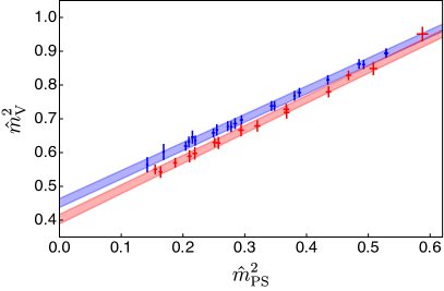
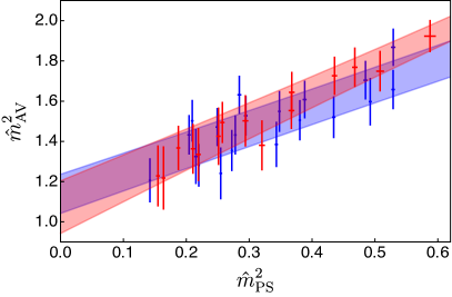
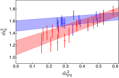
Figure 18: Meson masses squared from quenched (blue) and dynamical (red) calculations, in the continuum limit obtained by considering all the ensembles with $\hat{m}_{\rm PS}^{2}\mathrel{\raisebox{-2.32501pt}{$\stackrel{{\scriptstyle\textstyle<}}{{\sim}}$}}0.6$, as in Section 4.3. The coloured bands illustrate the fit of the measurements used in the massless extrapolations, with the width of the bands representing the statistical error in the fit.

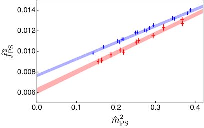
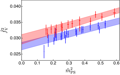
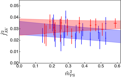
Figure 19: Meson decay constants squared from quenched (blue) and dynamical (red) calculations, in the continuum limit obtained by considering all the ensembles with $\hat{m}_{\rm PS}^{2}\mathrel{\raisebox{-2.32501pt}{$\stackrel{{\scriptstyle\textstyle<}}{{\sim}}$}}0.6$ for $\hat{f}_{\rm V}^{2}$ and $\hat{f}_{\rm AV}^{2}$, but restricting to $\hat{m}_{\rm PS}^{2}\mathrel{\raisebox{-2.32501pt}{$\stackrel{{\scriptstyle\textstyle<}}{{\sim}}$}}0.4$ for $\hat{f}_{\rm PS}^{2}$, as in Section 4.3. The coloured bands illustrate the fit of the measurements used in the massless extrapolations, with the width of the bands representing the statistical error in the fit.

We close this section by comparing the dynamical results to the quenched ones. Experience from lattice QCD suggests that the quenched results, which require only a small amount of computing resources, capture well the qualitative features of the dynamical results for masses and decay constants, in spite of the fact that the associated systematic uncertainties are not under analytical control. Quenching effects are expected to be smaller as the number of colours increases with a fixed number of fundamental flavours.

In order to make the comparison possible, our preliminary exploration of quenched simulations Bennett:2017kga had to be extended by considering larger lattice volumes and various lattice couplings Sp4ASFQ . As in the dynamical case, the quenched ensembles satisfy the condition $m_{\rm PS}L\gtrsim 7.5$, that allows one to neglect finite volume effects. Continuum extrapolations use ensembles constructed for $\beta=7.62$, $7.7$, $7.85$, $8.0$ and $8.2$. In contrast to the case of dynamical results—in which different ensembles are characterised by the choices of $\beta$ as well as $am_{0}$—only five independent ensembles generated at different $\beta$ values are used for all the quenched measurements. The results are hence affected by correlations among the data for various values of the fermion mass, which are obtained from the same ensemble, as well as from the continuum extrapolation carried out by using only five different values of the lattice spacing. The uncertainties associated with these systematic effects were estimated by varying the fitting intervals in the continuum and massless extrapolations. The numerical details and results of this quenched calculations are presented in Ref. Sp4ASFQ .

In Figs. 18 and 19, we show together the continuum extrapolated data both for quenched and dynamical fermions, restricted to the linear-mass regime—to $\hat{m}_{\rm PS}^{2}\mathrel{\raisebox{-2.58334pt}{$\stackrel{{\scriptstyle\textstyle<}}{{\sim}}$}}0.4$ for the pseudoscalar decay constant and to $\hat{m}_{\rm PS}^{2}\mathrel{\raisebox{-2.58334pt}{$\stackrel{{\scriptstyle\textstyle<}}{{\sim}}$}}0.6$ for masses and decay constants of all other mesons. As seen in the figures, $\hat{f}_{\rm PS}^{2}$ and $\hat{m}_{\rm S}^{2}$ are significantly affected by quenching, and the differences become more substantial as the fermion mass decreases. We estimate the discrepancies to be $\delta_{\hat{f}_{\rm PS}^{2}}/\hat{f}_{\rm PS}^{2}\sim 20\%$ and $\delta_{\hat{m}_{\rm S}^{2}}/\hat{m}_{\rm S}^{2}\sim 25\%$, in the massless limit. The mass of the V meson shows a somewhat milder discrepancy, at the level of $\sim 10\%$. For other quantities, quenching effects are not visible: the corresponding discrepancies are smaller than the uncertainties associated with the fits. Interestingly, the resulting values of $\hat{m}_{\rm V}/\sqrt{2}\hat{f}_{\rm PS}$ for the dynamical and quenched simulations, which may be used to estimate the coupling $g_{\rm VPP}$ via the second KSRF relation, are found to be consistent with each other in the massless limit Sp4ASFQ . The general conclusion of the comparison with the quenched results is quite encouraging, although at present we do not know whether this conclusion is an indication that the quenched approximation adequately captures the information encoded in the two-point functions—possibly because of the proximity to large-$N$—or whether it is just a trivial consequence of the large fermion masses we studied.

8 Continuum results: summary

In this section, we briefly summarise the continuum extrapolation results for the dynamical theory, presented in Section 6 and 7.

• Our continuum results for the decay constants and masses of PS, V, and AV states, for the ensembles satisfying $\hat{m}_{\rm PS}^{2}\leq 0.4$, are reported, in units of the gradient flow scale, in Table 9.

• The global fit based on the EFT describing PS, V and AV states using hidden local symmetry yields the results in Table 10, illustrated in Figs. 12 and 13.

• Section 6.1 discusses the GMOR relation and three sum rules in the continuum limit. The main results are shown in Figs. 14 and 15.

• In Section 7 the continuum limit results are discussed in units of the decay constant $f_{\rm PS}$ of the PS states, that are summarised in Table 11, and illustrated in Fig. 16. We include also the mass of the scalar flavoured state S. All our measurements are in the range $1.39\mathrel{\raisebox{-2.58334pt}{$\stackrel{{\scriptstyle\textstyle<}}{{\sim}}$}}\hat{m}_{\rm V}/\hat{m}_{\rm PS}\mathrel{\raisebox{-2.58334pt}{$\stackrel{{\scriptstyle\textstyle<}}{{\sim}}$}}1.87$, in which the V states cannot decay to states containing two PS particles. (Analogous considerations apply to the 3-body decay of the AV mesons.) This range may be of direct relevance in the context of dark matter models.

• We perform the extrapolation to the massless limit. The masses of V, AV, and S states are $m_{\rm V}/f_{\rm PS}=8.08(32)$, $m_{\rm AV}/f_{\rm PS}=13.4(1.5)$, and $m_{\rm S}/f_{\rm PS}=14.2(1.7)$. The decay constants of V and AV states in the continuum and massless limit are $f_{\rm V}/f_{\rm PS}=2.15(8)$ and $f_{\rm AV}/f_{\rm PS}=2.3(4)$, respectively—see Table 11.

• We find that $f_{\rm V}/f_{\rm PS}=2.15(8)$ is larger than expected on the basis of the first KSRF relation, which would yield $f_{\rm V}=\sqrt{2}\,f_{\rm PS}$—see Section 7.

• The second KSRF relation is satisfied, with $g_{\rm VPP}=6.0(4)(2)$ from the global fit, and $m_{\rm V}/(\sqrt{2}f_{\rm PS})=5.72(18)(13)$ obtained from the massless limit extrapolation.

• We compare the continuum and massless limit results to the literature on theories with two Dirac fermions on the fundamental. Fig. 17 shows that the VPP coupling is smaller than in the $SU(2)$ theory, but comparable to $SU(3)$ and $SU(4)$.

• We close Section 7 by comparing our results, obtained with dynamical fermions, to quenched calculations Sp4ASFQ . (See Figures 18 and 19.) We find that, in the massless limit, the decay constant squared of the PS state $\hat{f}_{\rm PS}^{2}$ is $\sim 20\%$ lower than the quenched result. The mass squared of the (flavoured) scalar is $\sim 25\%$ lower than in the quenched result, while that of the vector is lower by $\sim 10\%$. In the other observables, the dynamical and quenched results are compatible with one another, given the current uncertainties.

9 Conclusions and outlook

Following along the programme outlined in Ref. Bennett:2017kga , with this paper we have made a substantial step forwards in the study of the gauge theory with $Sp(4)$ group and $N_{f}=2$ (Dirac) fundamental fermions, that at long distance yields pNGBs describing the $SU(4)/Sp(4)$ coset, of relevance in the CHM context. We have adopted the Wilson-Dirac lattice action for gauge and fermion degrees of freedom, and performed numerical studies via the HMC method, with dynamical fermions. We have repeated the calculations at several values of the lattice bare parameters (fermion mass and gauge coupling). Our main result is the first continuum extrapolation of the $Sp(4)$ measurements for the masses and decay constants of the lightest, flavoured, spin-0 and spin-1 mesons. While numerical studies are performed in a regime of fermion masses large enough to preclude the decay of heavier mesons to the pNGBs, we have presented also a preliminary massless extrapolation, and compared the results to those of the quenched approximation. Summaries of the lattice and continuum limit results can be found in the brief Sections 5 and 8, respectively. Other results of relevance to the broad research programme of lattice gauge theories with $Sp(2N)$ group will be reported in Refs. Sp4ASFQ and Sp2Nglue (see also Ref. Lee:2018ztv ).

In the CHM context, while it is not strictly necessary to have massless fermions, it would be important in the future to extend this study to reach closer to the massless regime, for pNGB masses that allow the heavier mesons to decay. This would allow to test whether the moderate departure of our results from the quenched ones is due to the large fermion mass in the action, to the approach to the large-$N$ limit, to dynamical properties of the theory or to a combination of the above. Of great importance in the CHM context is also the problem of vacuum alignment. A first step towards addressing this point, without specifying the full set of couplings to SM fermions, would be to compute the coefficients of higher-order operators in the EFT obtained by retaining only the pNGB degrees of freedom. This information could be used as input in model building, to compute the (perturbative) Higgs potential responsible for EWSB. In general, it would also be interesting to track the dependence on $N$ of the spectra of mesons in $Sp(2N)$ theories with the same fermion field content, and understand how closely it follows the expectations from the large-$N$ analysis.

The mass regime we studied is suitable for direct application in the context of models with strongly-coupled origin of dark matter (along the lines of Refs. Hochberg:2014dra ; Hochberg:2014kqa ; Berlin:2018tvf , for example). The information we provide here is a necessary first step towards adopting this theory as a candidate for the origin of dark matter. Further information about the dynamics feeds into the relevant cross-sections, the calculation of which requires knowing the interactions. The first coupling one would like to measure in the future is the $g_{\rm VPP}$ coupling between one vector state V and two pseudoscalar states PS. We have performed a preliminary determination of this coupling based upon the EFT constructed to include also V and AV mesons, but the intrinsic limitations of this process imply that the results should be used with some caution.

Finally, CHM constructions often involve advocating for (partial) compositeness of some of the SM fermions, the top quark in particular. To this purpose, model building requires the existence of new composite fermion states with special properties, that can be realised in the $Sp(4)$ gauge theory by introducing $n_{f}=3$ (Dirac) fermions transforming in the 2-index antisymmetric representation of the group Barnard:2013zea ; Ferretti:2013kya . Some results about the (quenched) spectrum of mesons in the theory with this field content will be presented in Ref. Sp4ASFQ , but the implementation of fully dynamical calculations with multiple fermion representations will require a significant amount of development, with only few examples of calculations of this type existing in the current literature DeGrand:2016pgq ; Ayyar:2017qdf ; Ayyar:2018zuk ; Ayyar:2018glg ; Cossu:2019hse .

Appendix A Lattice action and numerical calculations: additional details

We collect in this Appendix some supplementary details, pertaining the lattice numerical study that ultimately leads to the results summarised in Tables 6 and 7, which provide the data upon which we perform the continuum and massless extrapolations. In Appendix A.1 we discuss the treatment of the $Sp(2N)$ matrices within the HMC algorithm. We briefly clarify the role of diquark operators in Appendix A.2. Finally, in Appendix A.3 we present details of the fitting procedure of the correlation functions used to extract masses and decay constants.

A.1 Hybrid Monte Carlo

We perform numerical simulations using a variant of HiRep code DelDebbio:2008zf , which is designed to simulate $SU(N)$ and $SO(N)$ lattice gauge theories with fermions in higher representations. While a detailed description of the implementations of $Sp(2N)$ theories in the HiRep code is described in Ref. Bennett:2017kga (see also Refs. Bennett:2017tum and Bennett:2017kbp ), here we briefly summarise its main features and then report on some improvements we implemented for the purposes of this and future projects. This paper focuses on the spectroscopy of $Sp(4)$ with two fundamental fermions, higher-dimensional representations will be discussed elsewhere. To study the $N_{f}=2$ theory we use the standard hybrid Monte Carlo algorithm, a well established technique for lattice QCD.

In our preliminary study of the two-flavor $Sp(4)$ theory Bennett:2017kga , we used the specific form of group generators $T^{A}$ given in Ref. Lee:2017uvl with the normalisation of $\textrm{Tr}(T^{A}T^{B})=\delta^{AB}/2$ for the molecular dynamics (MD) evolution. We also implemented a resymplectisation process, to ensure that updated configurations stay inside the $Sp(4)$ group manifold, that requires performing a (normalised) group projection onto the quaternion basis. This process works well for $Sp(4)$ theories, but in order to enhance the capability of the software in view of future studies of dynamical $Sp(2N)$ theories with arbitrary $N$, in this study we further improve and generalise the code in the following way.

First, we remind the reader that the group elements $U$ of $Sp(2N)$ satisfy the condition

$$U^{*}=\Omega U\Omega^{\dagger},~{}~{}~{}\textrm{with}~{}\Omega = \left(\begin{array}[]{cc}0&\mathbb{I}_{N\times N}\cr-\mathbb{I}_{N\times N}&0\cr\end{array}\right)\,.$$ (49)

$U$ is a unitary matrix, and it can be written as $U=\textrm{exp}(ia^{A}T^{A})$, where $T^{A}$ are Hermitian traceless $2N\times 2N$ matrices, and $a^{N}$ real numbers. Combining Eq. (49) and unitarity, one can also write the matrix $U$ in the block-diagonal form:

$$U = \left(\begin{array}[]{cc}V&W\cr-W^{*}&V^{*}\cr\end{array}\right)\,,$$ (52)

where $V$ and $W$ are complex $N\times N$ matrices. Because of its adaptability to any $N$, we perform the resymplectisation via a variant of the modified Gram-Schmidt algorithm, that has been tested for the pure gauge model with Heath Bath algorithm Bennett:2017kbp ; Bennett:2017kga . The basic idea is that the ($N+j$)-th column of $U$ can be obtained from $j$-th via $col_{j+N}=-\Omega col_{j}$, while the Gram-Schimt procedure is used to find the ($j+1$)-th column through the orthonormalisation with respect to the $j$-th and ($N+j$)-th. We also modified the code to save two $N\times N$ matrices ($V$ and $W$), instead of the full $2N\times 2N$ unitary matrix $U$, reducing by half the size of each configuration.

The MD update in HMC makes explicit use of the generators of the group, not just of the group elements. We write the group generators $T^{A}$ as follows. Eq. (49) can be rewritten in terms of the group generator $T^{A}$, as the condition

$$T^{A*}=-\Omega T^{A}\Omega^{\dagger},$$ (53)

which allows to write $T^{A}$ in block-diagonal matrix form as

$$T^{A} = \left(\begin{array}[]{cc}X&Y\cr Y^{*}&-X^{*}\cr\end{array}\right)\,,$$ (56)

where of the two $N\times N$ matrices, $X$ is Hermitian and $Y$ is complex symmetric. We use the definition in Eq. (56), supplemented by the normalisation $\textrm{Tr}\,(T^{A}T^{B})=\delta^{AB}/2$, for the generators implemented into the HiRep code.

We conclude by summarising some technical details about the algorithm used in the $Sp(4)$ gauge theory with two Dirac fermions in the fundamental representation. Gauge configurations are generated using the HMC with a second order Omelyan integrator for the MD update. We use different lengths of MD time steps $\delta\tau_{g}$ and $\delta\tau_{f}$ for gauge and fermions actions, respectively, which are optimised to keep the acceptance rate of the Metropolis test, performed at the end of each HMC update, in the range of $75-85\%$. Thermalisation and autocorrelation lengths are determined by monitoring the average value of the plaquette.

A.2 Of diquarks

In the theory studied in this paper, mesons and diquarks combine together in the low-energy spectrum, to form irreducible representations after the spontaneous breaking of the enlarged global $SU(4)$ symmetry breaking to $Sp(4)$. Hence, we do not calculate the diquark correlators, as they are identical to the corresponding meson correlators. A general discussion of both real and pseudoreal representations can be found in Ref. DeGrand:2015lna , yet we think it is useful to explicitly write the diquark operators and show the identity at the level of correlators by using our lattice action in Eq. (4). Such an analysis for SU($2$) theory with two fundamental fermions can be found in Ref. Lewis:2011zb .

The diquark operators are defined by

$$\mathcal{O}_{D}(x)\equiv Q^{T}_{i}(x)(-\Omega)C\Gamma Q_{j}(x),$$ (57)

where $C$ is the charge conjugation operator satisfying $\gamma^{\mu T}C=-C\gamma^{\mu}$, $\Gamma$ is a generic matrix with spinor indices, spinor indices are understood and summed over, and the anti-symmetric matrix $\Omega$ defined in Eq. (49) acts on the (understood) colour indices. Then, the diquark correlation function is

$$C_{\mathcal{O}_{D}}(t) = \sum_{\vec{x}}\langle 0|\mathcal{O}_{D}(\vec{x},t)\mathcal{O}_{D}^{\dagger}(\vec{0},0)|0\rangle$$ (58)

$$= \sum_{\vec{x}}\textrm{Tr}\left[\Gamma S_{j}(x;0)\gamma^{0}\Gamma^{\dagger}C^{\dagger}(-\Omega)^{\dagger}\gamma^{0T}S_{i}^{T}(x;0)(-\Omega)C\right]$$

$$= -\sum_{\vec{x}}\textrm{Tr}\left[\Gamma S_{j}(x;0)\gamma^{0}\Gamma^{\dagger}\gamma^{0}C^{\dagger}(-\Omega)^{\dagger}S_{i}^{T}(x;0)(-\Omega)C\right].$$

The inverse of a quark propagator $S^{-1}$—or, equivalently, the Wilson-Dirac operator—can be obtained from Eq. (4):

$$S^{-1}_{i}(x;y)=(4+a\,m_{0})\delta_{x,y}-\frac{1}{2}\sum_{\mu}\left((1-\gamma_{\mu})U_{\mu}(x)\delta_{x+\hat{\mu},y}+(1+\gamma_{\mu})U^{\dagger}(x)\delta_{y,x-\hat{\mu}}\right).$$ (59)

By recalling Eq. (49) and the defining property of the charge-conjugation matrix $C^{-1}=C^{\dagger}=C^{T}=-C$, one can show that

$$C^{-1}(-\Omega)^{-1}(S^{-1}_{i}(x;y))^{T}(-\Omega)C=S^{-1}_{i}(y;x),$$ (60)

which in turn leads to

$$C^{\dagger}(-\Omega)^{\dagger}S^{T}_{i}(x;y)(-\Omega)C=S_{i}(y;x).$$ (61)

Combining this result with Eq. (19) and Eq. (58), we finally arrive at

$$C_{\mathcal{O}_{D}}(t)=C_{\mathcal{O}_{M}}(t)\,,$$ (62)

where $C_{\mathcal{O}_{M}}(t)$ is the meson correlation function defined in Eq. (19).

Ensemble	$N_{\rm configs}$	$\delta_{\rm traj}$	PS		V		AV
			$I_{\rm fit}$	$\chi^{2}/N_{\rm d.o.f}$	$I_{\rm fit}$	$\chi^{2}/N_{\rm d.o.f.}$	$I_{\rm fit}$	$\chi^{2}/N_{\rm d.o.f.}$
DB1M1	100	24	9-16	0.3	10-16	0.4	6-10	1.3
DB1M2	100	24	11-16	0.8	9-16	0.2	6-9	0.1
DB1M3	100	24	10-16	0.5	10-16	1.0	6-10	1.1
DB1M4	74	32	10-16	1.1	10-16	0.2	6-9	0.9
DB1M5	183	12	10-16	0.6	10-15	1.0	7-10	0.6
DB1M6	80	28	10-16	0.7	10-16	0.3	6-9	0.5
DB1M7	71	12	10-16	0.5	10-16	1.3	7-10	0.5
DB2M1	100	20	12-18	0.8	11-18	0.5	8-11	1.1
DB2M2	100	24	12-18	0.5	13-18	0.6	8-14	0.6
DB2M3	102	20	13-18	1.0	12-16	0.4	9-11	0.1
DB3M1	120	20	14-18	0.5	14-18	0.2	8-12	0.3
DB3M2	100	24	12-18	0.6	12-18	0.8	8-14	1.0
DB3M3	200	12	13-18	1.0	13-17	1.0	9-15	0.4
DB3M4	200	12	14-17	0.7	14-18	0.7	9-15	0.9
DB3M5	150	12	15-18	0.3	15-18	0.8	9-15	1.3
DB3M6	200	12	13-18	0.8	13-17	0.1	10-15	0.6
DB3M7	199	12	14-18	0.6	14-18	0.8	9-14	1.4
DB3M8	150	12	15-20	0.6	15-20	0.9	10-16	0.2
DB4M1	150	12	19-24	1.0	15-24	1.9	12-17	0.6
DB4M2	150	12	19-23	0.4	17-24	0.6	12-15	0.2
DB5M1	105	12	16-24	0.6	18-24	0.2	11-19	0.6

Table 12: Fitting intervals of the Euclidean time $I_{\rm fit}=[t_{i},t_{f}]$ used in the single-exponential fit of the measured correlators for PS, V and AV mesons. The number of configurations and the separation between the adjacent configurations are denoted by $N_{\rm configs}$ and $\delta_{\rm traj}$, respectively. We carry out a correlated fit using standard $\chi^{2}$ minimisation. We show the resulting values of $\chi^{2}/N_{\rm d.o.f.}$, as a way to assess the quality of the fit itself.

Ensemble	T		AT		S
	$I_{\rm fit}$	$\chi^{2}/N_{\rm d.o.f}$	$I_{\rm fit}$	$\chi^{2}/N_{\rm d.o.f.}$	$I_{\rm fit}$	$\chi^{2}/N_{\rm d.o.f.}$
DB1M1	9-16	1.1	6-10	0.8	6-9	1.7
DB1M2	9-16	0.9	6-9	0.9	6-9	0.4
DB1M3	8-16	1.0	6-10	1.6	7-10	0.6
DB1M4	10-16	1.4	6-10	1.0	5-8	1.2
DB1M5	10-16	0.4	6-10	0.6	7-10	0.7
DB1M6	9-16	0.7	7-10	1.6	6-9	0.5
DB1M7	8-16	0.5	7-10	0.8	6-10	0.1
DB2M1	11-18	0.7	8-12	0.6	8-13	0.4
DB2M2	12-18	1.5	8-12	1.6	7-9	1.0
DB2M3	11-18	1.0	9-11	1.1	7-12	0.3
DB3M1	14-18	0.2	7-12	0.4	9-14	0.9
DB3M2	12-18	0.9	7-13	1.5	8-14	1.0
DB3M3	13-18	0.8	8-14	0.9	8-14	0.2
DB3M4	11-18	1.2	10-15	0.4	9-16	0.5
DB3M5	13-18	0.4	10-14	1.4	9-15	0.7
DB3M6	12-17	0.1	10-15	0.7	10-15	1.2
DB3M7	13-18	0.6	9-16	1.6	9-15	0.9
DB3M8	11-20	0.4	10-14	1.0	10-17	1.7
DB4M1	15-24	0.4	11-16	1.1	12-18	0.5
DB4M2	16-24	0.7	12-16	0.2	11-17	0.5
DB5M1	18-24	0.6	11-19	0.2	11-20	1.3

Table 13: Fitting intervals of the Euclidean time $I_{\rm fit}=[t_{i},t_{f}]$ used in the single-exponential fit of the measured correlators for T, AT and S mesons, where the same $N_{\rm configs}$ and $\delta_{\rm traj}$ in Table 12 are considered. We carry out a correlated fit using standard $\chi^{2}$ minimisation. We show the resulting values of $\chi^{2}/N_{\rm d.o.f.}$, as a way to assess the quality of the fit itself.

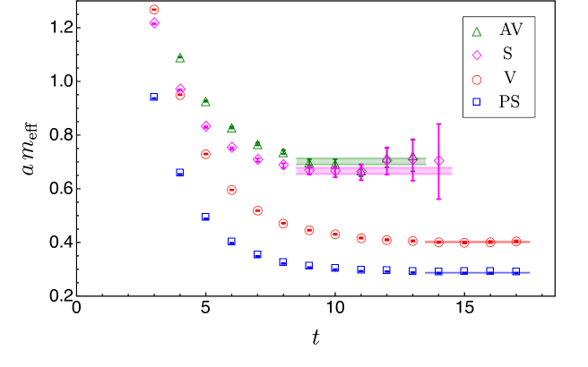
Figure 20: Example of effective mass plots of low-lying spin-$0$ and spin-$1$ mesons. The data is taken from the DB3M7 ensemble (see list in Table 1), which is characterised by the lattice parameters $\beta=7.2$ and $am_{0}=-0.794$. The individual fits that yield the masses of the PS, V, S and AV states are restricted to include only the plateau regions, which are highlighted by the shaded bands. The width of each band represents for the statistical uncertainty.

A.3 Effective mass and fitting procedure

In order to extract the lattice measurements of masses and decay constants, we fit the numerical data for the relevant two-point correlation functions. In all ensembles we produced, the Euclidean time is large enough to reach a plateau region in the plot of $m_{\rm eff}$ versus time $t$, in which the correlation functions are well approximated by a single exponential function, with its decay rate identified by the mass of mesons—the relevant 2-point function asymptotically behaves as $C_{{\cal O}_{M}}(t)\propto e^{-m_{\rm M}t}$. We use standard $\chi^{2}$ minimisation to this functional form to determine the best fit parameters (mass and decay constant, in units of the lattice spacing) and their statistical uncertainties.

This process requires choosing, for each ensemble and each meson, an interval $I_{\rm fit}=[t_{i},t_{f}]$ of Euclidean time, and restricting the fit to data collected between its minimum value $t_{i}$ and its maximum time $t_{f}$. We choose the fitting intervals as follows: we first look at the effective mass plots and identify the emergence of the plateau. Over the plateau region, we perform a single-exponential fit. We vary the choices of $t_{i}$ and $t_{f}$, and ultimately identify the best fit range with the choice that yields the smallest value for $\chi^{2}/N_{\rm d.o.f}$, with the largest possible range $t_{f}-t_{i}$. We provide the relevant details of this process in Tables 12 and 13. As an illustrative example, in Fig. 20 we show the effective mass plots for PS, V, AV and S mesons at $\beta=7.2$ and $am_{0}=-0.794$ (corresponding to ensemble DB3M7). The shaded bands represent the fit results, showing both the statistical uncertainties (width of the band) and the best fitting ranges (length of the band). For the PS meson, we perform a simultaneous fit of the two-point functions of PS and AV operators in Eq. (20) and Eq. (22).

We notice that while the effective masses retained in the fit extend to the maximum length of the temporal directions $T_{\rm max}$ for PS and V mesons, those for AV and S mesons typically cease at $t<T_{\rm max}$ due to severe numerical noise problems, which in practical terms reduce the fitting ranges. As a result, we expect a comparatively large systematic error associated with the choice of the fitting range for AV and S states (analogous arguments apply to the AT states).

Appendix B Low-energy constants and global fit

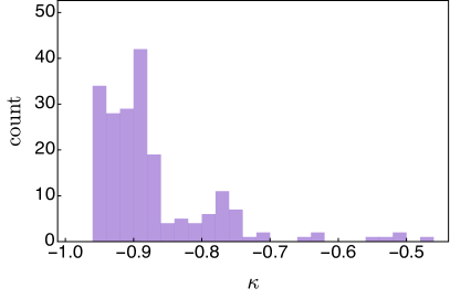
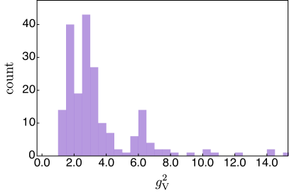
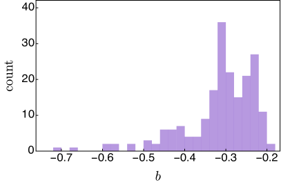
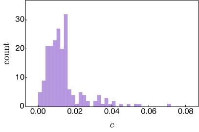
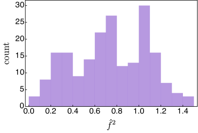
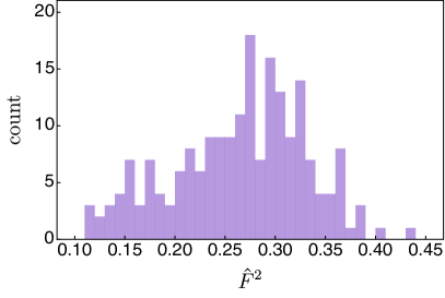
Figure 21: Histograms of the distribution of the six low-energy constants appearing in the EFT of Section 6.1 at the leading order, as determined from the global fit.

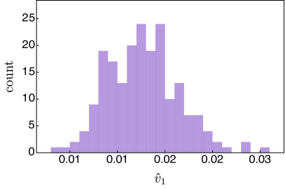
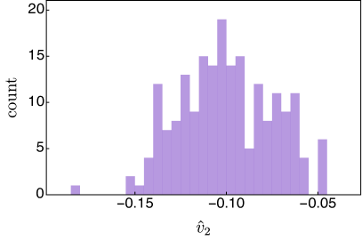
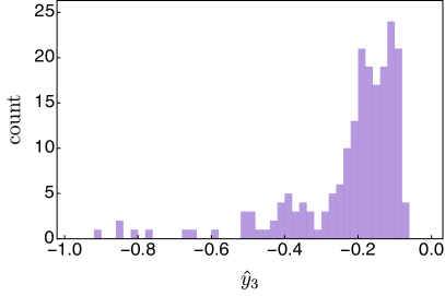
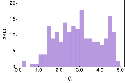
Figure 22: Histograms of the distribution of the four low-energy constants appearing in the EFT of Section 6.1 at the next-to-the-leading order, as determined from the global fit.

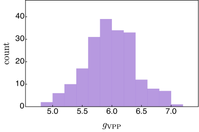
Figure 23: Histogram of derived quantity $g_{\rm VPP}$—see Eq. (40) in Section 6.1—based upon the distributions in Figs. 21 and 22.

In this Appendix, we present the numerical results for the LECs in Eqs. (32)-(6.1) obtained from the simplified global fit to the data discussed in Section 6.1. As anticipated, we find it instructive to explicitly show the histograms associated with the LEC distributions. Figs. 21 and 22 report the histograms for the LECs appearing in the EFT at the leading and the next-to-the-leading order, respectively. As seen in the figures, some fit parameters do not exhibit gaussian distributions, but rather expose long, flat tails. The samples in the tail do not lead to big upwards fluctuations of the value of $\chi^{2}/N_{\rm{d.o.f}}$, suggesting that there are some local minima in the parameter space with $\chi^{2}$ close to the global minimum, or possibly a flat direction. Figure 23 shows the histogram for the $g_{\rm VPP}$ coupling as defined and discussed in Eq. (40) in Section 6.1.

References

- (1) G. Aad et al. [ATLAS Collaboration], “Observation of a new particle in the search for the Standard Model Higgs boson with the ATLAS detector at the LHC,” Phys. Lett. B 716, 1 (2012) doi:10.1016/j.physletb.2012.08.020 [arXiv:1207.7214 [hep-ex]].
- (2) S. Chatrchyan et al. [CMS Collaboration], “Observation of a new boson at a mass of 125 GeV with the CMS experiment at the LHC,” Phys. Lett. B 716, 30 (2012) doi:10.1016/j.physletb.2012.08.021 [arXiv:1207.7235 [hep-ex]].
- (3) D. B. Kaplan and H. Georgi, “SU(2) x U(1) Breaking by Vacuum Misalignment,” Phys. Lett. 136B, 183 (1984). doi:10.1016/0370-2693(84)91177-8
- (4) H. Georgi and D. B. Kaplan, “Composite Higgs and Custodial SU(2),” Phys. Lett. 145B, 216 (1984). doi:10.1016/0370-2693(84)90341-1
- (5) M. J. Dugan, H. Georgi and D. B. Kaplan, “Anatomy of a Composite Higgs Model,” Nucl. Phys. B 254, 299 (1985). doi:10.1016/0550-3213(85)90221-4
- (6) M. E. Peskin, “The Alignment of the Vacuum in Theories of Technicolor,” Nucl. Phys. B 175, 197 (1980). doi:10.1016/0550-3213(80)90051-6
- (7) K. Agashe, R. Contino and A. Pomarol, “The Minimal composite Higgs model,” Nucl. Phys. B 719, 165 (2005) doi:10.1016/j.nuclphysb.2005.04.035 [hep-ph/0412089].
- (8) R. Contino, L. Da Rold and A. Pomarol, “Light custodians in natural composite Higgs models,” Phys. Rev. D 75, 055014 (2007) doi:10.1103/PhysRevD.75.055014 [hep-ph/0612048].
- (9) R. Barbieri, B. Bellazzini, V. S. Rychkov and A. Varagnolo, “The Higgs boson from an extended symmetry,” Phys. Rev. D 76, 115008 (2007) doi:10.1103/PhysRevD.76.115008 [arXiv:0706.0432 [hep-ph]].
- (10) P. Lodone, “Vector-like quarks in a ’composite’ Higgs model,” JHEP 0812, 029 (2008) doi:10.1088/1126-6708/2008/12/029 [arXiv:0806.1472 [hep-ph]].
- (11) D. Marzocca, M. Serone and J. Shu, “General Composite Higgs Models,” JHEP 1208, 013 (2012) doi:10.1007/JHEP08(2012)013 [arXiv:1205.0770 [hep-ph]].
- (12) C. Grojean, O. Matsedonskyi and G. Panico, JHEP 1310, 160 (2013) doi:10.1007/JHEP10(2013)160 [arXiv:1306.4655 [hep-ph]].
- (13) G. Ferretti and D. Karateev, “Fermionic UV completions of Composite Higgs models,” JHEP 1403, 077 (2014) doi:10.1007/JHEP03(2014)077 [arXiv:1312.5330 [hep-ph]].
- (14) G. Cacciapaglia and F. Sannino, “Fundamental Composite (Goldstone) Higgs Dynamics,” JHEP 1404, 111 (2014) doi:10.1007/JHEP04(2014)111 [arXiv:1402.0233 [hep-ph]].
- (15) A. Arbey, G. Cacciapaglia, H. Cai, A. Deandrea, S. Le Corre and F. Sannino, “Fundamental Composite Electroweak Dynamics: Status at the LHC,” Phys. Rev. D 95, no. 1, 015028 (2017) doi:10.1103/PhysRevD.95.015028 [arXiv:1502.04718 [hep-ph]].
- (16) L. Vecchi, “A dangerous irrelevant UV-completion of the composite Higgs,” JHEP 1702, 094 (2017) doi:10.1007/JHEP02(2017)094 [arXiv:1506.00623 [hep-ph]].
- (17) G. Panico and A. Wulzer, “The Composite Nambu-Goldstone Higgs,” Lect. Notes Phys. 913, pp.1 (2016) doi:10.1007/978-3-319-22617-0 [arXiv:1506.01961 [hep-ph]].
- (18) G. Ferretti, “Gauge theories of Partial Compositeness: Scenarios for Run-II of the LHC,” JHEP 1606, 107 (2016) doi:10.1007/JHEP06(2016)107 [arXiv:1604.06467 [hep-ph]].
- (19) A. Agugliaro, O. Antipin, D. Becciolini, S. De Curtis and M. Redi, “UV complete composite Higgs models,” Phys. Rev. D 95, no. 3, 035019 (2017) doi:10.1103/PhysRevD.95.035019 [arXiv:1609.07122 [hep-ph]].
- (20) T. Alanne, D. Buarque Franzosi and M. T. Frandsen, “A partially composite Goldstone Higgs,” Phys. Rev. D 96, no. 9, 095012 (2017) doi:10.1103/PhysRevD.96.095012 [arXiv:1709.10473 [hep-ph]].
- (21) F. Feruglio, B. Gavela, K. Kanshin, P. A. N. Machado, S. Rigolin and S. Saa, “The minimal linear sigma model for the Goldstone Higgs,” JHEP 1606, 038 (2016) doi:10.1007/JHEP06(2016)038 [arXiv:1603.05668 [hep-ph]].
- (22) S. Fichet, G. von Gersdorff, E. Pontón and R. Rosenfeld, “The Excitation of the Global Symmetry-Breaking Vacuum in Composite Higgs Models,” JHEP 1609, 158 (2016) doi:10.1007/JHEP09(2016)158 [arXiv:1607.03125 [hep-ph]].
- (23) J. Galloway, A. L. Kagan and A. Martin, “A UV complete partially composite-pNGB Higgs,” Phys. Rev. D 95, no. 3, 035038 (2017) doi:10.1103/PhysRevD.95.035038 [arXiv:1609.05883 [hep-ph]].
- (24) T. Alanne, D. Buarque Franzosi, M. T. Frandsen, M. L. A. Kristensen, A. Meroni and M. Rosenlyst, “Partially composite Higgs models: Phenomenology and RG analysis,” JHEP 1801, 051 (2018) doi:10.1007/JHEP01(2018)051 [arXiv:1711.10410 [hep-ph]].
- (25) C. Csaki, T. Ma and J. Shu, “Maximally Symmetric Composite Higgs Models,” Phys. Rev. Lett. 119, no. 13, 131803 (2017) doi:10.1103/PhysRevLett.119.131803 [arXiv:1702.00405 [hep-ph]].
- (26) M. Chala, G. Durieux, C. Grojean, L. de Lima and O. Matsedonskyi, “Minimally extended SILH,” JHEP 1706, 088 (2017) doi:10.1007/JHEP06(2017)088 [arXiv:1703.10624 [hep-ph]].
- (27) C. Csaki, T. Ma and J. Shu, “Trigonometric Parity for Composite Higgs Models,” Phys. Rev. Lett. 121, no. 23, 231801 (2018) doi:10.1103/PhysRevLett.121.231801 [arXiv:1709.08636 [hep-ph]].
- (28) V. Ayyar, T. Degrand, D. C. Hackett, W. I. Jay, E. T. Neil, Y. Shamir and B. Svetitsky, “Baryon spectrum of SU(4) composite Higgs theory with two distinct fermion representations,” Phys. Rev. D 97, no. 11, 114505 (2018) doi:10.1103/PhysRevD.97.114505 [arXiv:1801.05809 [hep-ph]].
- (29) V. Ayyar, T. DeGrand, D. C. Hackett, W. I. Jay, E. T. Neil, Y. Shamir and B. Svetitsky, “Finite-temperature phase structure of SU(4) gauge theory with multiple fermion representations,” Phys. Rev. D 97, no. 11, 114502 (2018) doi:10.1103/PhysRevD.97.114502 [arXiv:1802.09644 [hep-lat]].
- (30) C. Cai, G. Cacciapaglia and H. H. Zhang, “Vacuum alignment in a composite 2HDM,” arXiv:1805.07619 [hep-ph].
- (31) A. Agugliaro, G. Cacciapaglia, A. Deandrea and S. De Curtis, “Vacuum misalignment and pattern of scalar masses in the SU(5)/SO(5) composite Higgs model,” arXiv:1808.10175 [hep-ph].
- (32) V. Ayyar, T. DeGrand, D. C. Hackett, W. I. Jay, E. T. Neil, Y. Shamir and B. Svetitsky, “Partial compositeness from baryon matrix elements on the lattice,” arXiv:1812.02727 [hep-ph].
- (33) G. Cacciapaglia, S. Vatani, T. Ma and Y. Wu, “Towards a fundamental safe theory of composite Higgs and Dark Matter,” arXiv:1812.04005 [hep-ph].
- (34) O. Witzel, “Review on Composite Higgs Models,” arXiv:1901.08216 [hep-lat].
- (35) G. Cacciapaglia, G. Ferretti, T. Flacke and H. Serôdio, “Light scalars in composite Higgs models,” Front. Phys. 7, 22 (2019) doi:10.3389/fphy.2019.00022 [arXiv:1902.06890 [hep-ph]].
- (36) V. Ayyar, M. F. Golterman, D. C. Hackett, W. Jay, E. T. Neil, Y. Shamir and B. Svetitsky, “Radiative Contribution to the Composite-Higgs Potential in a Two-Representation Lattice Model,” Phys. Rev. D 99, no. 9, 094504 (2019) doi:10.1103/PhysRevD.99.094504 [arXiv:1903.02535 [hep-lat]].
- (37) G. Cossu, L. Del Debbio, M. Panero and D. Preti, “Strong dynamics with matter in multiple representations: SU(4) gauge theory with fundamental and sextet fermions,” Eur. Phys. J. C 79, no. 8, 638 (2019) doi:10.1140/epjc/s10052-019-7137-1 [arXiv:1904.08885 [hep-lat]].
- (38) G. Cacciapaglia, H. Cai, A. Deandrea and A. Kushwaha, “Fundamental Composite Higgs model in SU(6)/SO(6),” arXiv:1904.09301 [hep-ph].
- (39) D. Buarque Franzosi and G. Ferretti, “Anomalous dimensions of potential top-partners,” arXiv:1905.08273 [hep-ph].
- (40) E. Katz, A. E. Nelson and D. G. E. Walker, “The Intermediate Higgs,” JHEP 0508, 074 (2005) doi:10.1088/1126-6708/2005/08/074 [hep-ph/0504252].
- (41) B. Gripaios, A. Pomarol, F. Riva and J. Serra, “Beyond the Minimal Composite Higgs Model,” JHEP 0904, 070 (2009) doi:10.1088/1126-6708/2009/04/070 [arXiv:0902.1483 [hep-ph]].
- (42) J. Barnard, T. Gherghetta and T. S. Ray, “UV descriptions of composite Higgs models without elementary scalars,” JHEP 1402, 002 (2014) doi:10.1007/JHEP02(2014)002 [arXiv:1311.6562 [hep-ph]].
- (43) R. Lewis, C. Pica and F. Sannino, “Light Asymmetric Dark Matter on the Lattice: SU(2) Technicolor with Two Fundamental Flavors,” Phys. Rev. D 85, 014504 (2012) doi:10.1103/PhysRevD.85.014504 [arXiv:1109.3513 [hep-ph]].
- (44) A. Hietanen, R. Lewis, C. Pica and F. Sannino, “Fundamental Composite Higgs Dynamics on the Lattice: SU(2) with Two Flavors,” JHEP 1407, 116 (2014) doi:10.1007/JHEP07(2014)116 [arXiv:1404.2794 [hep-lat]].
- (45) R. Arthur, V. Drach, M. Hansen, A. Hietanen, C. Pica and F. Sannino, “SU(2) gauge theory with two fundamental flavors: A minimal template for model building,” Phys. Rev. D 94, no. 9, 094507 (2016) doi:10.1103/PhysRevD.94.094507 [arXiv:1602.06559 [hep-lat]].
- (46) R. Arthur, V. Drach, A. Hietanen, C. Pica and F. Sannino, “ Gauge Theory with Two Fundamental Flavours: Scalar and Pseudoscalar Spectrum,” arXiv:1607.06654 [hep-lat].
- (47) C. Pica, V. Drach, M. Hansen and F. Sannino, “Composite Higgs Dynamics on the Lattice,” EPJ Web Conf. 137, 10005 (2017) doi:10.1051/epjconf/201713710005 [arXiv:1612.09336 [hep-lat]].
- (48) W. Detmold, M. McCullough and A. Pochinsky, “Dark nuclei. II. Nuclear spectroscopy in two-color QCD,” Phys. Rev. D 90, no. 11, 114506 (2014) doi:10.1103/PhysRevD.90.114506 [arXiv:1406.4116 [hep-lat]].
- (49) J. W. Lee, B. Lucini and M. Piai, “Symmetry restoration at high-temperature in two-color and two-flavor lattice gauge theories,” JHEP 1704, 036 (2017) doi:10.1007/JHEP04(2017)036 [arXiv:1701.03228 [hep-lat]].
- (50) G. Cacciapaglia, H. Cai, A. Deandrea, T. Flacke, S. J. Lee and A. Parolini, “Composite scalars at the LHC: the Higgs, the Sextet and the Octet,” JHEP 1511, 201 (2015) doi:10.1007/JHEP11(2015)201 [arXiv:1507.02283 [hep-ph]].
- (51) N. Bizot, M. Frigerio, M. Knecht and J. L. Kneur, “Nonperturbative analysis of the spectrum of meson resonances in an ultraviolet-complete composite-Higgs model,” Phys. Rev. D 95, no. 7, 075006 (2017) doi:10.1103/PhysRevD.95.075006 [arXiv:1610.09293 [hep-ph]].
- (52) D. K. Hong, “Very light dilaton and naturally light Higgs boson,” JHEP 1802, 102 (2018) doi:10.1007/JHEP02(2018)102 [arXiv:1703.05081 [hep-ph]].
- (53) M. Golterman and Y. Shamir, “Effective potential in ultraviolet completions for composite Higgs models,” Phys. Rev. D 97, no. 9, 095005 (2018) doi:10.1103/PhysRevD.97.095005 [arXiv:1707.06033 [hep-ph]].
- (54) V. Drach, T. Janowski and C. Pica, “Update on SU(2) gauge theory with NF = 2 fundamental flavours,” EPJ Web Conf. 175, 08020 (2018) doi:10.1051/epjconf/201817508020 [arXiv:1710.07218 [hep-lat]].
- (55) F. Sannino, P. Stangl, D. M. Straub and A. E. Thomsen, “Flavor Physics and Flavor Anomalies in Minimal Fundamental Partial Compositeness,” Phys. Rev. D 97, no. 11, 115046 (2018) doi:10.1103/PhysRevD.97.115046 [arXiv:1712.07646 [hep-ph]].
- (56) T. Alanne, N. Bizot, G. Cacciapaglia and F. Sannino, “Classification of NLO operators for composite Higgs models,” Phys. Rev. D 97, no. 7, 075028 (2018) doi:10.1103/PhysRevD.97.075028 [arXiv:1801.05444 [hep-ph]].
- (57) N. Bizot, G. Cacciapaglia and T. Flacke, “Common exotic decays of top partners,” JHEP 1806, 065 (2018) doi:10.1007/JHEP06(2018)065 [arXiv:1803.00021 [hep-ph]].
- (58) D. Buarque Franzosi, G. Cacciapaglia and A. Deandrea, “Sigma-assisted natural composite Higgs,” arXiv:1809.09146 [hep-ph].
- (59) H. Gertov, A. E. Nelson, A. Perko and D. G. E. Walker, “Lattice-Friendly Gauge Completion of a Composite Higgs with Top Partners,” arXiv:1901.10456 [hep-ph].
- (60) E. Bennett, D. K. Hong, J. W. Lee, C.-J. D. Lin, B. Lucini, M. Piai and D. Vadacchino, “Sp(4) gauge theory on the lattice: towards SU(4)/Sp(4) composite Higgs (and beyond),” JHEP 1803, 185 (2018) doi:10.1007/JHEP03(2018)185 [arXiv:1712.04220 [hep-lat]].
- (61) E. Bennett, D. K. Hong, J. W. Lee, C.-J. D. Lin, B. Lucini, M. Piai and D. Vadacchino, “Higgs compositeness in Sp(2N) gauge theories—Resymplecticisation, scale setting and topology,” EPJ Web Conf. 175, 08012 (2018) doi:10.1051/epjconf/201817508012 [arXiv:1710.06715 [hep-lat]].
- (62) E. Bennett, D. K. Hong, J. W. Lee, C.-J. D. Lin, B. Lucini, M. Piai and D. Vadacchino, “Higgs compositeness in Sp(2N) gauge theories—Determining the low-energy constants with lattice calculations,” EPJ Web Conf. 175, 08011 (2018) doi:10.1051/epjconf/201817508011 [arXiv:1710.06941 [hep-lat]].
- (63) E. Bennett, D. K. Hong, J. W. Lee, C.-J. D. Lin, B. Lucini, M. Piai and D. Vadacchino, “Higgs compositeness in Sp(2N) gauge theories—The pure gauge model,” EPJ Web Conf. 175, 08013 (2018) doi:10.1051/epjconf/201817508013 [arXiv:1710.07043 [hep-lat]].
- (64) J. W. Lee, E. Bennett, D. K. Hong, C.-J. D. Lin, B. Lucini, M. Piai and D. Vadacchino, “Progress in the lattice simulations of Sp(2N) gauge theories,” PoS LATTICE 2018, 192 (2018) [arXiv:1811.00276 [hep-lat]].
- (65) F. Sannino, Phys. Rev. D 79, 096007 (2009) doi:10.1103/PhysRevD.79.096007 [arXiv:0902.3494 [hep-ph]].
- (66) T. A. Ryttov and R. Shrock, Phys. Rev. D 96, no. 10, 105015 (2017) doi:10.1103/PhysRevD.96.105015 [arXiv:1709.05358 [hep-th]].
- (67) Y. Hochberg, E. Kuflik, T. Volansky and J. G. Wacker, “Mechanism for Thermal Relic Dark Matter of Strongly Interacting Massive Particles,” Phys. Rev. Lett. 113, 171301 (2014) doi:10.1103/PhysRevLett.113.171301 [arXiv:1402.5143 [hep-ph]].
- (68) Y. Hochberg, E. Kuflik, H. Murayama, T. Volansky and J. G. Wacker, “Model for Thermal Relic Dark Matter of Strongly Interacting Massive Particles,” Phys. Rev. Lett. 115, no. 2, 021301 (2015) doi:10.1103/PhysRevLett.115.021301 [arXiv:1411.3727 [hep-ph]].
- (69) A. Berlin, N. Blinov, S. Gori, P. Schuster and N. Toro, “Cosmology and Accelerator Tests of Strongly Interacting Dark Matter,” Phys. Rev. D 97, no. 5, 055033 (2018) doi:10.1103/PhysRevD.97.055033 [arXiv:1801.05805 [hep-ph]].
- (70) M. Luscher, “Signatures of unstable particles in finite volume,” Nucl. Phys. B 364, 237 (1991). doi:10.1016/0550-3213(91)90584-K
- (71) X. Feng, K. Jansen and D. B. Renner, “Resonance Parameters of the rho-Meson from Lattice QCD,” Phys. Rev. D 83, 094505 (2011) doi:10.1103/PhysRevD.83.094505 [arXiv:1011.5288 [hep-lat]].
- (72) C. Alexandrou et al., Phys. Rev. D 96, no. 3, 034525 (2017) doi:10.1103/PhysRevD.96.034525 [arXiv:1704.05439 [hep-lat]].
- (73) A. D. Gasbarro and G. T. Fleming, “Examining the Low Energy Dynamics of Walking Gauge Theory,” PoS LATTICE 2016, 242 (2017) doi:10.22323/1.256.0242 [arXiv:1702.00480 [hep-lat]].
- (74) M. Bando, T. Kugo, S. Uehara, K. Yamawaki and T. Yanagida, “Is rho Meson a Dynamical Gauge Boson of Hidden Local Symmetry?,” Phys. Rev. Lett. 54, 1215 (1985). doi:10.1103/PhysRevLett.54.1215
- (75) R. Casalbuoni, S. De Curtis, D. Dominici and R. Gatto, “Effective Weak Interaction Theory with Possible New Vector Resonance from a Strong Higgs Sector,” Phys. Lett. 155B, 95 (1985). doi:10.1016/0370-2693(85)91038-X
- (76) M. Bando, T. Kugo and K. Yamawaki, “Nonlinear Realization and Hidden Local Symmetries,” Phys. Rept. 164, 217 (1988). doi:10.1016/0370-1573(88)90019-1
- (77) R. Casalbuoni, S. De Curtis, D. Dominici, F. Feruglio and R. Gatto, “Vector and Axial Vector Bound States From a Strongly Interacting Electroweak Sector,” Int. J. Mod. Phys. A 4, 1065 (1989). doi:10.1142/S0217751X89000492
- (78) M. Harada and K. Yamawaki, “Hidden local symmetry at loop: A New perspective of composite gauge boson and chiral phase transition,” Phys. Rept. 381, 1 (2003) doi:10.1016/S0370-1573(03)00139-X [hep-ph/0302103].
- (79) H. Georgi, “Vector Realization of Chiral Symmetry,” Nucl. Phys. B 331, 311 (1990). doi:10.1016/0550-3213(90)90210-5
- (80) T. Appelquist, P. S. Rodrigues da Silva and F. Sannino, “Enhanced global symmetries and the chiral phase transition,” Phys. Rev. D 60, 116007 (1999) doi:10.1103/PhysRevD.60.116007 [hep-ph/9906555].
- (81) M. Piai, A. Pierce and J. G. Wacker, “Composite vector mesons from QCD to the little Higgs,” hep-ph/0405242.
- (82) D. Buarque Franzosi, G. Cacciapaglia, H. Cai, A. Deandrea and M. Frandsen, “Vector and Axial-vector resonances in composite models of the Higgs boson,” JHEP 1611, 076 (2016) doi:10.1007/JHEP11(2016)076 [arXiv:1605.01363 [hep-ph]].
- (83) E. Bennett, D. K. Hong, J. W. Lee, M. Mesiti, C.-J. D. Lin, B. Lucini, M. Piai, J. Rantaharju and D. Vadacchino, “Sp(4) gauge theories on the lattice: quenched fundamental and antisymmetric fermions”, in preparation.
- (84) O. Bar and M. Golterman, “Chiral perturbation theory for gradient flow observables,” Phys. Rev. D 89, no. 3, 034505 (2014) Erratum: [Phys. Rev. D 89, no. 9, 099905 (2014)] doi:10.1103/PhysRevD.89.099905, 10.1103/PhysRevD.89.034505 [arXiv:1312.4999 [hep-lat]].
- (85) V. Ayyar, T. DeGrand, M. Golterman, D. C. Hackett, W. I. Jay, E. T. Neil, Y. Shamir and B. Svetitsky, “Spectroscopy of SU(4) composite Higgs theory with two distinct fermion representations,” Phys. Rev. D 97, no. 7, 074505 (2018) doi:10.1103/PhysRevD.97.074505 [arXiv:1710.00806 [hep-lat]].
- (86) B. Sheikholeslami and R. Wohlert, “Improved Continuum Limit Lattice Action for QCD with Wilson Fermions,” Nucl. Phys. B 259, 572 (1985). doi:10.1016/0550-3213(85)90002-1
- (87) G. Rupak and N. Shoresh, “Chiral perturbation theory for the Wilson lattice action,” Phys. Rev. D 66, 054503 (2002) doi:10.1103/PhysRevD.66.054503 [hep-lat/0201019].
- (88) S. R. Sharpe and R. L. Singleton, Jr, “Spontaneous flavor and parity breaking with Wilson fermions,” Phys. Rev. D 58, 074501 (1998) doi:10.1103/PhysRevD.58.074501 [hep-lat/9804028].
- (89) M. Luscher, S. Sint, R. Sommer and P. Weisz, “Chiral symmetry and O(a) improvement in lattice QCD,” Nucl. Phys. B 478, 365 (1996) doi:10.1016/0550-3213(96)00378-1 [hep-lat/9605038].
- (90) K. Symanzik, “Continuum Limit and Improved Action in Lattice Theories. 1. Principles and Theory,” Nucl. Phys. B 226, 187 (1983). doi:10.1016/0550-3213(83)90468-6
- (91) L. Del Debbio, A. Patella and C. Pica, “Higher representations on the lattice: Numerical simulations. SU(2) with adjoint fermions,” Phys. Rev. D 81, 094503 (2010) doi:10.1103/PhysRevD.81.094503 [arXiv:0805.2058 [hep-lat]].
- (92) K. Holland, M. Pepe and U. J. Wiese, “The Deconfinement phase transition of Sp(2) and Sp(3) Yang-Mills theories in (2+1)-dimensions and (3+1)-dimensions,” Nucl. Phys. B 694, 35 (2004) doi:10.1016/j.nuclphysb.2004.06.026 [hep-lat/0312022].
- (93) L. Del Debbio, M. T. Frandsen, H. Panagopoulos and F. Sannino, “Higher representations on the lattice: Perturbative studies,” JHEP 0806, 007 (2008) doi:10.1088/1126-6708/2008/06/007 [arXiv:0802.0891 [hep-lat]].
- (94) Bradley Efron, CBMS-NSF Regional Conference Series in Applied Mathematics, Philadelphia: Society for Industrial and Applied Mathematics (SIAM), 1982.
- (95) M. Lüscher, “Properties and uses of the Wilson flow in lattice QCD,” JHEP 1008, 071 (2010) Erratum: [JHEP 1403, 092 (2014)] doi:10.1007/JHEP08(2010)071, 10.1007/JHEP03(2014)092 [arXiv:1006.4518 [hep-lat]].
- (96) M. Lüscher and P. Weisz, “Perturbative analysis of the gradient flow in non-abelian gauge theories,” JHEP 1102, 051 (2011) doi:10.1007/JHEP02(2011)051 [arXiv:1101.0963 [hep-th]].
- (97) S. Borsanyi et al., “High-precision scale setting in lattice QCD,” JHEP 1209, 010 (2012) doi:10.1007/JHEP09(2012)010 [arXiv:1203.4469 [hep-lat]].
- (98) J. Gasser and H. Leutwyler, “Light Quarks at Low Temperatures,” Phys. Lett. B 184, 83 (1987). doi:10.1016/0370-2693(87)90492-8
- (99) M. Golterman, “Applications of chiral perturbation theory to lattice QCD,” arXiv:0912.4042 [hep-lat].
- (100) Z. Fodor, K. Holland, J. Kuti, D. Nogradi and C. H. Wong, “The Yang-Mills gradient flow in finite volume,” JHEP 1211, 007 (2012) doi:10.1007/JHEP11(2012)007 [arXiv:1208.1051 [hep-lat]].
- (101) L. Y. Glozman, “Restoration of chiral and U(1)A symmetries in excited hadrons,” Phys. Rept. 444, 1 (2007) doi:10.1016/j.physrep.2007.04.001 [hep-ph/0701081].
- (102) L. Y. Glozman and M. Pak, “Exploring a new SU(4) symmetry of meson interpolators,” Phys. Rev. D 92, no. 1, 016001 (2015) doi:10.1103/PhysRevD.92.016001 [arXiv:1504.02323 [hep-lat]].
- (103) L. Glozman, “Chiralspin Symmetry and Its Implications for QCD,” Universe 5, no. 1, 38 (2019) doi:10.3390/universe5010038 [arXiv:1810.09886 [hep-ph]].
- (104) P. A. Boyle, A. Juttner, C. Kelly and R. D. Kenway, “Use of stochastic sources for the lattice determination of light quark physics,” JHEP 0808, 086 (2008) doi:10.1088/1126-6708/2008/08/086 [arXiv:0804.1501 [hep-lat]].
- (105) T. DeGrand, Y. Liu, E. T. Neil, Y. Shamir and B. Svetitsky, “Spectroscopy of SU(4) gauge theory with two flavors of sextet fermions,” Phys. Rev. D 91, 114502 (2015) doi:10.1103/PhysRevD.91.114502 [arXiv:1501.05665 [hep-lat]].
- (106) G. Martinelli and Y. C. Zhang, “The Connection Between Local Operators on the Lattice and in the Continuum and Its Relation to Meson Decay Constants,” Phys. Lett. 123B, 433 (1983). doi:10.1016/0370-2693(83)90987-5
- (107) G. P. Lepage and P. B. Mackenzie, “On the viability of lattice perturbation theory,” Phys. Rev. D 48, 2250 (1993) doi:10.1103/PhysRevD.48.2250 [hep-lat/9209022].
- (108) M. Gell-Mann, R. J. Oakes and B. Renner, “Behavior of current divergences under SU(3) x SU(3),” Phys. Rev. 175, 2195 (1968). doi:10.1103/PhysRev.175.2195
- (109) J. Bijnens and J. Lu, “Technicolor and other QCD-like theories at next-to-next-to-leading order,” JHEP 0911, 116 (2009) doi:10.1088/1126-6708/2009/11/116 [arXiv:0910.5424 [hep-ph]].
- (110) S. Weinberg, “Precise relations between the spectra of vector and axial vector mesons,” Phys. Rev. Lett. 18, 507 (1967). doi:10.1103/PhysRevLett.18.507
- (111) T. DeGrand and Y. Liu, Phys. Rev. D 94, no. 3, 034506 (2016) Erratum: [Phys. Rev. D 95, no. 1, 019902 (2017)] doi:10.1103/PhysRevD.95.019902, 10.1103/PhysRevD.94.034506 [arXiv:1606.01277 [hep-lat]].
- (112) K. Jansen et al. [ETM Collaboration], “Meson masses and decay constants from unquenched lattice QCD,” Phys. Rev. D 80, 054510 (2009) doi:10.1103/PhysRevD.80.054510 [arXiv:0906.4720 [hep-lat]].
- (113) K. Kawarabayashi and M. Suzuki, “Partially conserved axial vector current and the decays of vector mesons,” Phys. Rev. Lett. 16, 255 (1966). doi:10.1103/PhysRevLett.16.255
- (114) Riazuddin and Fayyazuddin, “Algebra of current components and decay widths of rho and K* mesons,” Phys. Rev. 147, 1071 (1966). doi:10.1103/PhysRev.147.1071
- (115) M. Tanabashi et al. [Particle Data Group], “Review of Particle Physics,” Phys. Rev. D 98, no. 3, 030001 (2018). doi:10.1103/PhysRevD.98.030001
- (116) D. Nogradi and L. Szikszai, “The flavor dependence of ,” JHEP 1905, 197 (2019) doi:10.1007/JHEP05(2019)197 [arXiv:1905.01909 [hep-lat]].
- (117) E. Bennett, J. Holligan, D. K. Hong, J. W. Lee, C.-J. D. Lin, B. Lucini, M. Piai, and D. Vadacchino, “Sp(2N) Yang-Mills theories on the lattice: glueballs and strings”, in preparation.
- (118) T. DeGrand, M. Golterman, E. T. Neil and Y. Shamir, “One-loop Chiral Perturbation Theory with two fermion representations,” Phys. Rev. D 94, no. 2, 025020 (2016) doi:10.1103/PhysRevD.94.025020 [arXiv:1605.07738 [hep-ph]].