Supplementary matarial to “Confinement and lack of thermalization after quenches in bosonic Schwinger model”

.1 Derivation of the Hamiltonian

The Lagrangian density for the BSM Peskin and Schroeder (1995) is given by

$$\mathcal{L}=-\left[D_{\mu}\phi\right]^{*}D^{\mu}\phi-m^{2}|\phi|^{2}-\frac{1}{4}F_{\mu\nu}F^{\mu\nu},$$ (1)

where $\phi$ is the complex scalar field, $D_{\mu}=(\partial_{\mu}+iqA_{\mu})$ is the covariant derivative with $q$ and $A_{\mu}$ being the electronic charge and electromagnetic vector potential respectively, $m$ is the mass of the particles, and $F_{\mu\nu}$ is the electromagnetic field tensor. Here, we use the metric convection $(-1,1,1,1)$ or $(-1,1)$ (in 1+1 dimensions). In 1+1 dimensions, after fixing the temporal gauge $A_{t}(x,t)=0$, we get the quantum Hamiltonian as

$$\hat{H} = \int dx\bigg{[}\frac{1}{2}\hat{E}_{x}^{2}(x)+\hat{\Pi}^{\dagger}(x)\hat{\Pi}(x)+m^{2}\hat{\phi}^{\dagger}(x)\hat{\phi}(x)$$ (2)

$$+ \left(\partial_{x}-iq\hat{A}_{x}(x)\right)\hat{\phi}^{\dagger}(x)\left(\partial_{x}+iq\hat{A}_{x}(x)\right)\hat{\phi}(x)\bigg{]},$$

where $\hat{E}_{x}(x)$, $\hat{\Pi}(x)$, and $\hat{\Pi}^{\dagger}(x)$ are the canonical conjugate operators corresponding to $\hat{A}_{x}(x)$, $\hat{\phi}(x)$, and $\hat{\phi}^{\dagger}(x)$ respectively, satisfying $[\hat{A}_{x}(x_{1}),\hat{E}_{x}(x_{2})]=[\hat{\phi}(x_{1}),\hat{\Pi}(x_{2})]=[\hat{\phi}^{\dagger}(x_{1}),\hat{\Pi}^{\dagger}(x_{2})]=i\delta(x_{1}-x_{2})$. We can discretize this Hamiltonian on a 1D lattice having lattice-spacing $a$ in a straightforward way such that the matter fields $\{\hat{\phi}_{j},\hat{\phi}_{j}^{\dagger},\hat{\Pi}_{j},\hat{\Pi}_{j}^{\dagger}\}$ reside on lattice site $j$, while the gauge fields $\{\hat{A}_{j},\hat{E}_{j}\}$ act on the bonds between lattice points, e.g. $j$ and $j+1$. The Hamiltonian, thus discretized, reads as

$$\hat{H} = \frac{a}{2}\sum_{j}\hat{E}_{j}^{2}+\frac{1}{a}\sum_{j}\hat{\Pi}_{j}^{\dagger}\hat{\Pi}_{j}+\left(am^{2}+\frac{2}{a}\right)\sum_{j}\hat{\phi}_{j}^{\dagger}\hat{\phi}_{j}$$ (3)

$$- \frac{1}{a}\sum_{j}\left[\hat{\phi}_{j+1}^{\dagger}\exp(-iq\hat{A}_{j})\hat{\phi_{j}}+\mbox{ h.c.}\right],$$

where the operators have been rescaled to satisfy the commutation relations $[\hat{A}_{j},\hat{E}_{k}]=\ [\hat{\phi}_{j},\hat{\Pi}_{k}]=[\hat{\phi}^{\dagger}_{j},\hat{\Pi}^{\dagger}_{k}]=i\delta_{jk}$. In the next few steps, we introduce bosonic operators $\hat{a}_{j}$ and $\hat{b}_{j}$ as

$$\hat{\phi}_{j}=\frac{1}{\sqrt{2}}\left(\hat{a}_{j}+\hat{b}_{j}^{\dagger}\right),\ \hat{\Pi}_{j}=\frac{i}{\sqrt{2}}\left(\hat{a}^{\dagger}_{j}-\hat{b}_{j}\right),$$

$$\hat{\phi}^{\dagger}_{j}=\frac{1}{\sqrt{2}}\left(\hat{a}^{\dagger}_{j}+\hat{b}_{j}\right),\ \hat{\Pi}^{\dagger}_{j}=\frac{i}{\sqrt{2}}\left(\hat{b}^{\dagger}_{j}-\hat{a}_{j}\right),$$ (4)

rescale the gauge fields as $\hat{L}_{j}=\hat{E}_{j}/q,\ \hat{\theta}_{j}=q\hat{A}_{j}$, and multiply the Hamiltonian by $1/aq^{2}$ to make it dimensionless. The Hamiltonian now becomes

$$\hat{H} = \sum_{j}\hat{L}_{j}^{2}+\left((m/q)^{2}+3x\right)\sum_{j}\big{(}\hat{a}_{j}^{\dagger}\hat{a}_{j}+\hat{b}_{j}\hat{b}_{j}^{\dagger}\big{)}$$ (5)

$$+ \left((m/q)^{2}+x\right)\sum_{j}\big{(}\hat{a}_{j}^{\dagger}\hat{b}_{j}^{\dagger}+\hat{a}_{j}\hat{b}_{j}\big{)}$$

$$- x\sum_{j}\left[\big{(}\hat{a}^{\dagger}_{j+1}+\hat{b}_{j+1}\big{)}\hat{U}_{j}\big{(}\hat{a}_{j}+\hat{b}^{\dagger}_{j}\big{)}+\text{h.c.}\right],$$

where $\hat{U}_{j}=\exp(-i\hat{\theta_{j}})$ and $\hat{U}^{\dagger}_{j}=\exp(i\hat{\theta_{j}})$ are the ladder operators satisfying $[\hat{L}_{j},\hat{U}_{j}]=-\hat{U}_{j}$ and $\ [\hat{L}_{j},\hat{U}^{\dagger}_{j}]=\hat{U}^{\dagger}_{j}$ respectively, and $x=1/a^{2}q^{2}$. To further simplify the Hamiltonian, we employ a local Bogoliubov transformation as

$$\hat{a}_{j} \rightarrow \cosh(\theta_{j})\ \hat{a}_{j}+\sinh(\theta_{j})\ \hat{b}_{j}^{\dagger},$$

$$\hat{b}_{j} \rightarrow \cosh(\theta_{j})\ \hat{b}_{j}+\sinh(\theta_{j})\ \hat{a}_{j}^{\dagger},$$ (6)

where $\theta_{j}=-\frac{1}{2}\tanh^{-1}\left[\frac{\left(m/q\right)^{2}+x}{\left(m/q\right)^{2}+3x}\right]$ for all $j$, such that our final Hamiltonian is given as

$$\hat{H}=\sum_{j}\hat{L}_{j}^{2}+2\left(x\left(\left(m/q\right)^{2}+2x\right)\right)^{1/2}\ \sum_{j}\big{(}\hat{a}_{j}^{\dagger}\hat{a}_{j}+\hat{b}_{j}\hat{b}_{j}^{\dagger}\big{)}-\frac{x^{3/2}}{\left(\left(m/q\right)^{2}+2x\right)^{1/2}}\sum_{j}\left[\big{(}\hat{a}^{\dagger}_{j+1}+\hat{b}_{j+1}\big{)}\hat{U}_{j}\big{(}\hat{a}_{j}+\hat{b}^{\dagger}_{j}\big{)}+\text{h.c.}\right].$$ (7)

We refer the bosons ‘$a$’ and ‘$b$’ as particles and antiparticles respectively.

.2 Local gauge invariance and Gauss law generators

It can be straightforwardly verified that the Hamiltonian in Eq. (7) is invariant under local $U(1)$ gauge transformations:

$$\hat{a}_{j}\rightarrow e^{i\alpha_{j}}\ \hat{a}_{j},\ \hat{b}_{j}\rightarrow e^{-i\alpha_{j}}\ \hat{b}_{j},$$ (8)

$$\hat{U}_{j}\rightarrow e^{-i\alpha_{j}}\ \hat{U}_{j}\ e^{i\alpha_{j+1}}.$$ (9)

Corresponding Gauss law generators can be obtained from the Euler-Lagrange equation of the field $A_{t}$, i.e.,

$$\left[\partial_{\mu}\left[\frac{\partial\mathcal{L}}{\partial(\partial_{\mu}A_{t})}\right]-\frac{\partial\mathcal{L}}{\partial A_{t}}\right]_{A_{t}\rightarrow 0}=0,$$

$$\Rightarrow\partial_{x}E_{x}(x)=iq\left(\phi^{*}(x)\Pi^{*}(x)-\phi(x)\Pi(x)\right),$$ (10)

which, after quantization with normal ordering and discretization similar to the Hamiltonian, gives us the Gauss law generators as

$$\hat{G}_{j}=\hat{L}_{j}-\hat{L}_{j-1}-\underbrace{\left(\hat{a}_{j}^{\dagger}\hat{a}_{j}-\hat{b}_{j}^{\dagger}\hat{b}_{j}\right)}_{\hat{Q}_{j}},$$ (11)

where the dynamical charge, $\hat{Q}_{j}=\hat{a}_{j}^{\dagger}\hat{a}_{j}-\hat{b}_{j}^{\dagger}\hat{b}_{j}$, is basically the difference between the particle-antiparticle number. In the absence of any background static charges, the physical sector is spanned by the states satisfying $\hat{G}_{j}=0$ for all values of $j$. Using this constraint imposed by the Gauss law, we can integrate-out the gauge-fields for a chain with open-boundary condition using the following transformation,

$$\left[\prod_{l<j}\hat{U}_{l}\right]\hat{a}_{j}\rightarrow\hat{a}_{j},\ \left[\prod_{l<j}\hat{U}^{\dagger}_{l}\right]\hat{b}_{j}\rightarrow\hat{b}_{j},\hat{L}_{j}=\sum_{l\leq j}\hat{Q}_{l},$$ (12)

where the background static field at the left of the chain has been considered to be zero.

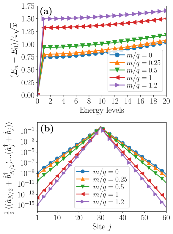
Figure 1: (Color online.) Energy levels of 20 low-lying states for different values of $m/q$ as obtained from the DMRG calculation. Clearly, the ground states are well-separated from the energy bands even in the massless case due the matter-gauge interaction, responsible for opening of mass-gaps. (b) Exponentially decaying correlation in the ground states of the system. Here, we plot the long-range correlation, $\frac{1}{2}\braket{(\hat{a}_{N/2}+\hat{b}^{\dagger}_{N/2})...(\hat{a}^{\dagger}_{j}+\hat{b}_{j})}$, as a function of distance $j$ from the middle of the chain, i.e., site $N/2$. Note that the ellipsis $...$ is to be replaced by proper Wilson lines to make the long-range operators gauge-invariant.

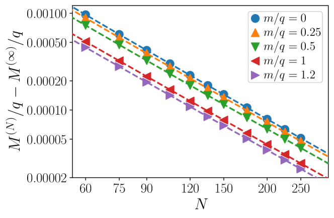
Figure 2: (Color online.) Finite-size scaling of mass-gap for different values of $m/q$. Here, we fit the values of mass-gaps obtained for different system-sizes to Eq. (15) to obtain the thermodynamic limits. The symbols represent the numerical data, the dashed lines show the fitted results. Error of these fits are of the order of $10^{-7}$ (for smaller masses) to $10^{-9}$ (for higher masses). All quantities plotted are dimensionless.

.3 Ground-state, mass-gap, and energy spectrum

.3.1 Energy spectrum in the non-interacting scenario

If we drop the $\sum_{j}\hat{L}_{j}^{2}$ term from the Hamiltonian (Eq. (7)), then the system is basically the discretized version of free (complex) Klein-Gordon (KG) theory in $1+1$ dimension, which can be solved exactly. After successive application of Fourier and Bogoliubov transformations, the non-interacting KG Hamiltonian, corresponding to the Hamiltonian of Eq. (7), boils down to

$$\hat{H}_{free}=\sum_{k}\omega_{k}\left(\hat{a}_{k}^{\dagger}\hat{a}_{k}+\hat{b}_{k}^{\dagger}\hat{b}_{k}+1\right),$$ (13)

where the doubly degenerate spectrum of the KG system is given by the dispersion relation

$$\omega_{k}=2\sqrt{xm^{2}/q^{2}+2x^{2}(1-\cos ka)},$$ (14)

for both the particles and the antiparticles. This dispersion relation is transformed into the relativistic one in the continuum limit as $\lim_{a\rightarrow 0}\frac{aq^{2}}{2}\omega_{k}=\sqrt{k^{2}+m^{2}}$. Note that for very low momentum excitations, i.e., $ka\ll 1$, the system also possesses Lorentz invariant dispersion even for finite size-size with finite lattice-spacing. Clearly, the ground state of the non-interacting system, which is the bare vacuum of the KG theory, is gapless for massless bosons and gapped otherwise, and the energy gap is given by, $\Delta E=2\times 2\sqrt{x}m/q$, where a factor of $2$ is needed as the excitations are in the from of ‘free’ boson-antiboson pairs.

.3.2 Emergence of mass-gap and binding energy

In presence of $\sum_{j}\hat{L}_{j}^{2}$ term in the Hamiltonian, excitations come in the form of bound particle-antiparticle pairs (mesons), and a finite mass-gap is generated due to the matter-gauge coupling. The mass-gap, i.e., the difference in energies between the ground and first excited states $M/q=(E_{1}-E_{0})/4\sqrt{x}$, is always larger than $m/q$, where the extra energy, $E_{B}/q=M/q-m/q$ arises in the from of binding energy required to tether particle-antiparticle pairs into mesons. In Fig. 1(a), we plot energies (as measured from the ground state energy) of 20 low-lying states as obtained from the DMRG calculation that shows the existence of mass-gap in the system. Due to this mass-gap, the ground state of the system is finitely correlated. Fig. 1(b) shows that long-range correlations decay exponentially with the distance in the ground state.

We move on with our analysis by extracting the information about mass-gap $M/q$ and the corresponding binding-energy, $E_{B}/q=M/q-m/q$, in the thermodynamic limit by finite-size scaling. Due to the open boundary condition, the mass-gaps will receive a kinetic energy correction with a leading contribution being $O(1/N^{2})$ as we approach the thermodynamic limit Hamer et al. (1997). Here, we consider the contributions upto $O(1/N^{3})$ perturbation term, so that the scaling is given by

$$M^{(N)}/q=M^{(\infty)}/q+\alpha_{1}/N^{2}+\alpha_{2}/N^{3},$$ (15)

where $\alpha_{1}$ and $\alpha_{2}$ are dimensionless constants. We obtain the values of the mass-gap from DMRG calculation for different system-sizes $N\in[60,250]$, and numerically fit the data to Eq. (15) (see Fig. 2) to get the mass-gap in the thermodynamic limit. In Table 1, we list the values of mass-gaps and corresponding binding energies in the thermodynamic limit for different values of $m/q$.

$m/q$	Mass-gap, $M/q$	Binding energy, $E_{B}/q$
0	0.74688	0.74688
0.25	0.79872	0.55872
0.5	0.93303	0.53303
1	1.32112	0.32112
1.2	1.49636	0.29636

Table 1: Mass-gaps and binding energies for $x=2$ in the thermodynamic limit as extracted from the finite-size scaling.

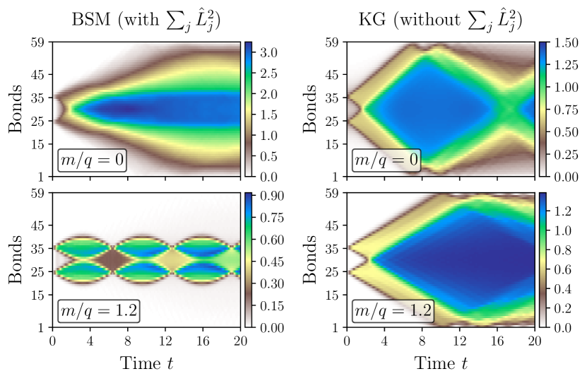
Figure 3: (Color online.) Dynamics of entanglement in the BSM (left column) and in the non-interacting KG system (right column). We plot the entanglement entropy of the time-evolved state after subtracting the entropy of respective ground state $\ket{\Omega}$ and consider $R=5$.

.4 Entanglement dynamics

In the main text, we have presented the time profile for classical and distillable part of the entanglement entropy. Here, we supplement those results with the profile of the total entanglement entropy $\mathcal{S}_{j}(t)$ measured across every bond $j$ and compare it with what is observed in a non-interacting KG system, obtained by dropping $\sum_{j}\hat{L}^{2}_{j}$ term from the Hamiltonian.

Fig. 3 shows $S_{j}(t)$ for the interacting BSM (left column), and the the non-interacting KG model (right column) for all bonds $j$. For the KG model the entanglement spreads linearly with a light-cone structure as predicted by the pseudo-particle picture. For a given $j\ll N/2$, it initially increases ballistically with time and saturates to a value proportional to the volume of the region as predicted by Calabrese and Cardy (2005) and is recently discussed in the context of generalized thermalization Rigol et al. (2008); Vidmar and Rigol (2016). The particles bouncing off the boundaries induce the observed recurrences.

In the BSM, the spread of the entanglement is strongly modified by the effects of confinement (left column). Initially its spreading slows-down, and only starts to spread ballistically in correspondence to the radiation of free mesons for lighter masses. Furthermore, most of the entanglement is contained in the region that is initially occupied by the confined bosonic matter, and persists there even long after the concentration of bosons in the bulk disappears at around $t\simeq 10$. On the other hand, the concentration of entanglement never leaks into the deconfined domain for heavier bosons, e.g., $m/q=1.2$. Such unusual dynamics of entanglement gives us yet another indicator of strong reluctance towards thermalization.

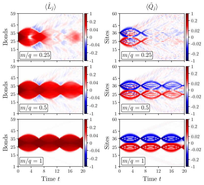
Figure 4: (Color online.) Dynamics of electric field $\braket{\hat{L_{j}}}$ (left column) and dynamical charge $\braket{\hat{Q}_{j}}$ (right column) for $m/q=2.5$ (top row), $0.5$ (middle row), and $1$ (bottom row) and $R=5$.

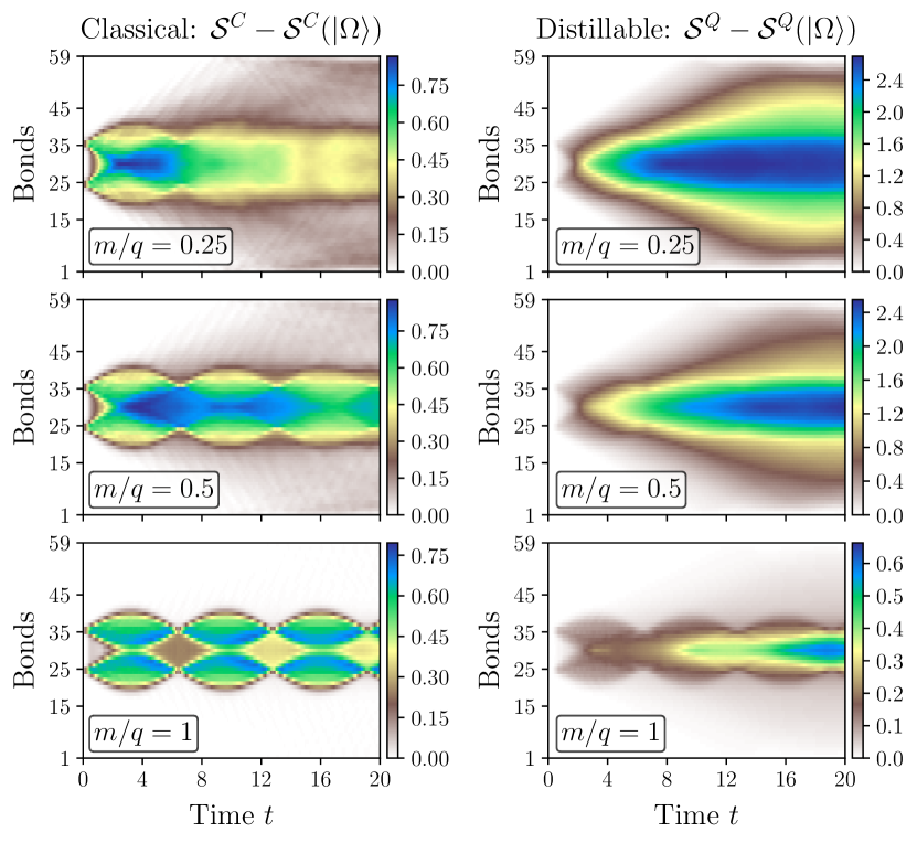
Figure 5: (Color online.) Time-evolution the classical part $\mathcal{S}^{C}$ of entanglement entropy (left column) and the distillable entanglement entropy $\mathcal{S}^{Q}$ (right column) for $m/q=2.5$ (top row), $0.5$ (middle row), and $1$ (bottom row) and $R=5$.

.5 Dynamics for intermediate boson masses

In the main text, we have presented the out-of-equilibrium dynamics for two extreme values of boson mass, namely $m/q=0$ and $1.2$. Here, we supplement those results by showing the dynamics for intermediate values of $m/q$. Fig. 4 shows the dynamics of both the gauge sector ($\hat{L}_{j}$) and the charge sector ($\hat{Q}_{j}$) for boson masses $m/q=0.25$, $0.5$, and $1$ for $R=5$. Clearly, as the mass increases the confining behavior of the dynamics becomes stronger, as the coherent oscillation of the confined core lasts longer. For example, there is no string-inversion for $m/q=0.25$ before $t=8$, and the string does not break in the bulk for $m/q=0.5$. On the other hand, we already reach the heavy boson limit with $m/q=1$.

The classical ($\mathcal{S}^{C}$) and the distillable ($\mathcal{S}^{Q}$) parts of entanglement entropy shows similar features for these intermediate masses (Fig. 5). The distinction between the deconfined domain and the confined core, as perceived from the classical part, becomes much more pronounced for $m/q=0.25$ and $0.5$ than the massless scenario depicted in the main text.

.6 Area-law of entanglement entropy in the confined domain

As mentioned in the main text, we follow the entanglement dynamics for system sizes $N=60$, $80$, and $100$ with $R=N/10$ so that the initial string length increases with the system size. The average entropy in the confined domain, i.e.,

$$\mathcal{S}^{Av}=\frac{1}{2R+1}\sum_{j=N/2-R}^{N/2+R}\mathcal{S}_{j}$$ (16)

follows the area-law of entanglement throughout the dynamics as it remains (almost) invariant with the system size as shown in Fig. 6 for $M/q=0$ and $0.25$. Here, the entropy grows rapidly and reaches its maximum value at $t\approx 10$ and then starts to decay slowly similar to the situation of larger masses at much later times that we have seen in the main text.

The area-law of entanglement entropy can be also perceived from the entanglement profile of the systems at long times. In Fig. 7 we depict the entanglement profile for $m/q=1.2$ at $t=200$ for $N=60$ and $R=5$. Clearly, the entropy in the central confined region remains almost invariant with the size of the bipartition, and the region just outside this central region starts to show a linear increase of entanglement entropy with the size of the bipartition.

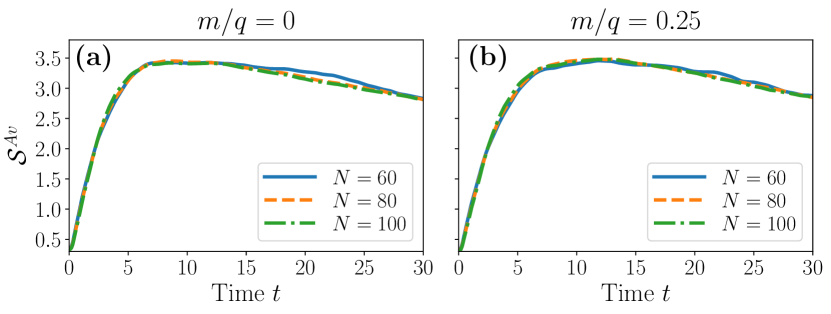
Figure 6: (Color online.) Evolution of average entropy in the confined domain for different system sizes. Here we consider $R=N/10$ so that it grows proportional to the system size.

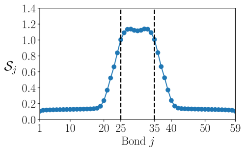
Figure 7: (Color online.) The entanglement profile for $m/q=1.2$ at time $t=200$. Here, we consider $N=60$ and $R=5$. The region inside the dashed lines refers to the central confined region.

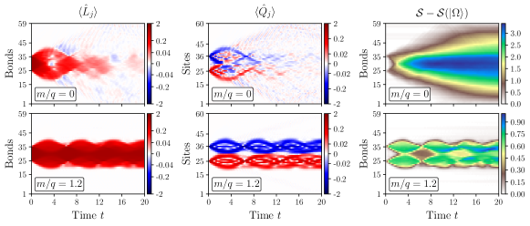
Figure 8: (Color online.) Dynamics of the electric field $\braket{\hat{L}_{j}}$, the dynamical charge $\braket{\hat{Q}_{j}}$, and entanglement entropy $\mathcal{S}_{j}$ for $R=5$ and $m/q=0$ under random on-site disorder. Random on-site potential $\sum_{j}\mu_{j}\left(\hat{a}_{j}^{\dagger}\hat{a}+\hat{b}_{j}^{\dagger}\hat{b}\right)$ has been added to the system where $\mu_{j}$ has been chosen randomly in between $[-1/2,1/2]$.

.7 Robustness of confining dynamics under random noise

Here, we show that the confining dynamics described in the main text is robust under random noises that may be present in the system. For that purpose, we add on-site random potential $\mu_{j}\sum_{j}\left(\hat{a}_{j}^{\dagger}\hat{a}_{j}+\hat{b}_{j}^{\dagger}\hat{b}_{j}\right)$ to the Hamiltonian, where $\mu_{j}$ is chosen randomly from $\left[-1/2,1/2\right]$. Fig. 8 shows an instance for one such dynamical behavior for the massless case. Although the profile of the light cones get deformed due to random disorder, the confining dynamics can be easily grasp from the bending of the trajectories of the bosons. More importantly, the entanglement entropy remains concentrated on the central region like in the clean case, thereby indicating a strong memory effect and thus lack of thermalization.

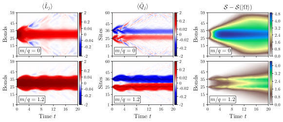
Figure 9: Dynamics of the electric field $\braket{\hat{L}_{j}}$, the dynamical charge $\braket{\hat{Q}_{j}}$, and entanglement entropy $\mathcal{S}_{j}$ for the initial state $\ket{\psi^{\prime}(t=0)}=\mathcal{N}^{\prime}\hat{M}^{2}_{R}\ket{\Omega}$, with $\mathcal{N}^{\prime}$ being the normalization constant and $R=5$.

.8 Confining dynamics at higher energies

We also probe the dynamics at a larger energy than the scenario presented in the main text. For that, we excite the ground state by acting the non-local string operator $\hat{M}_{R}$ twice, such that the initial state becomes, $\ket{\psi^{\prime}(t=0)}=\mathcal{N}^{\prime}\hat{M}_{R}^{2}\ket{\Omega}$, with $\mathcal{N}^{\prime}$ being the normalization constant. Semiclassically, this initial state has twice the extra energy than the previous scenario. In Fig. 9, we depict such dynamics of the electric field $\braket{\hat{L}_{j}}$, the dynamical charge $\braket{\hat{Q}_{j}}$, and entanglement entropy $\mathcal{S}_{j}$ for $m/q=0$ and $1.2$. In spite of having more energy than the previous case, the memory effect becomes more prominent, as the concentration of bosons remains localized in the central region for much longer time.

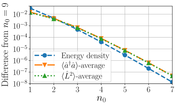
Figure 10: (Color online.) Dependence of physical quantities on the boson number cutoff $n_{0}$ in the ground state of the system for $m/q=0$. Here we plot the difference between the values of different observables computed for different values of $n_{0}$ from $n_{0}=9$. Clearly, for $n_{0}=5$ the error due to the truncated bosonic Hilbert space falls below $10^{-5}$.

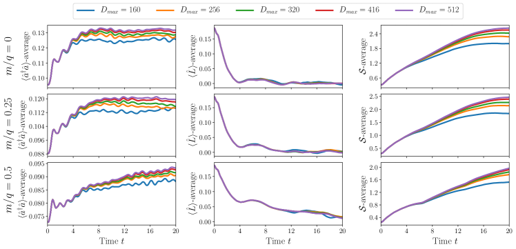
Figure 11: (Color online.) Time-evolution of different physical observables using hybrid TDVP for different bond-dimensions. We plot the averages of $\braket{\hat{a}^{\dagger}\hat{a}}$ (left column), $\braket{\hat{L}}$ (middle column), and the entanglement entropy $\mathcal{S}$ (right column) as function of time upto $t=20$ for $m/q=0$, $0.25$, and $0.5$.

.9 Details about tensor network simulation

We use matrix product states (MPS) Schollwöck (2011); Orús (2014) ansatz with open boundary condition to simulate states of the system, where we integrate-out the gauge fields using the Gauss law. Due to tracing-out of the gauge fields, we do not need to use gauge-invariant tensor network Tagliacozzo et al. (2014); Buyens et al. (2014); Silvi et al. (2014); Kull et al. (2017) for our calculations. However, we use global $U(1)$ symmetry Singh et al. (2010, 2011) corresponding to the conservation of the total dynamical charge, $\sum_{j}\hat{Q}_{j}$, and obviously we work only in the $\sum_{j}\braket{\hat{Q}_{j}}=0$ sector. The maximum number bosons ($n_{0}$) per site for each species has been truncated to 5, resulting in a physical dimension of 36 on each site. This truncation is justified as the densities of the bosons never cross $\sim 1.5$ throughout our simulation. We confirm this by checking the convergence of several observables with respect to $n_{0}$ in the ground-state of the model in Fig. 10, where we show that for $m/q=0$ the errors due to this truncation is below $10^{-5}$ for $n_{0}=5$. One important thing to mention here is that it is also possible to separate-out two types of bosons to odd and even lattice-sites respectively maintaining global $U(1)$ symmetry, such that physical dimension on each site only grows linearly with $n_{0}$. This will definitely increase efficiency of the simulation for a given MPS bond dimension. However, as two types of bosons sitting on a same site are strongly correlated, such a method of separating them out using truncated bonds will incur much more errors, especially in the time-evolution, and needs much larger bond dimension to get converged results.

To find the ground state of the system, first we use two-site density matrix renormalization group (DMRG) White (1992, 1993); Schollwöck (2005) upto a maximum bond dimension $D_{max}\leq 100$, so that largest SVD truncation error with $D_{max}$ remains below $10^{-12}$. After that we switch to one-site variational optimization (“one-site DMRG”) White (2005); Schollwöck (2011) for more stringent convergence within the MPS manifold given by $D_{max}$.

To obtain low-lying excited states, we employ the same method, where we shift the Hamiltonian each-time by a suitable weight factor multiplied with the projector of the previously found state, i.e., to find the $n^{th}$ excited state $\ket{\psi_{n}}$, we search for the ground state of the shifted Hamiltonian,

$$\hat{H}^{\prime}=\hat{H}+W\sum_{m=0}^{n-1}\ket{\psi_{m}}\bra{\psi_{m}},$$ (17)

where $W$ should be guessed to be sufficiently larger than $E_{n}-E_{0}$. In this scenario, $D_{max}=100$ is not always sufficient to reduce the SVD truncation error below $10^{-12}$ and that is why convergence from the one-site variational optimization procedure becomes absolutely necessary.

Time-evolution using MPS ansatz (tensor network in general) is always tricky, error-prone, and therefore must be dealt with caution, as entanglement entropy grows ballistically in the dynamics, which, in turn, demands larger and larger MPS bond dimension. Recently, to tackle such issues, the time-dependent variational principle (TDVP) algorithm Haegeman et al. (2011); Koffel et al. (2012); Haegeman et al. (2016) has been developed, which has been argued to be much less error-prone than earlier methods, e.g., time evolving block decimation (TEBD), within a given bond dimension Paeckel et al. (2019). Here we employ “hybrid” TDVP with step-size $\delta t=0.01$, where we first use two-site version of TDVP to dynamically grow the bond dimension upto $D_{max}=512$. When the bond dimension in the bulk of the MPS is saturated to $D_{max}=512$, we switch to the one-site version to avoid any error due to SVD truncation. This hybrid method of time-evolution using TDVP has been argued to incur much less error than other known methods Paeckel et al. (2019); Goto and Danshita (2019). It is noteworthy to mention here that since we use properly converged Lanczos exponentiation Hochbruck and Lubich (1997) in TDVP simulations, different step-sizes do not alter the results. To be assured of the trustworthiness of our simulations, we also perform TDVP simulations for $D_{max}=160$, $256$, $320$, and $416$ and check the convergence of different observables with respect to different $D_{max}$ (see Fig. 11 for the case of $N=60$ and $R=5$). Clearly, upto $t\approx 4$, all the graphs, including $D_{max}=160$ simulations, are converged, even when tallied in the light of entanglement entropy $\mathcal{S}$, which is believed to behave much worse in truncated bond dimensions. On the other hand, $D_{max}=416$ data remain satisfactorily close to $D_{max}=512$ curves throughout the time window, showing the reliability of our simulation with the bond dimension $D_{max}=512$. For heavier masses, e.g., $m/q=1.2$ (not shown in the figure), all the quantities are converged for every bond dimension considered here.

References

- Peskin and Schroeder (1995) M. E. Peskin and D. V. Schroeder, An introduction to quantum field theory (Addison-Wesley Pub. Co, Reading, Mass, 1995).
- Hamer et al. (1997) C. J. Hamer, Z. Weihong, and J. Oitmaa, Phys. Rev. D 56, 55 (1997).
- Calabrese and Cardy (2005) P. Calabrese and J. Cardy, Journal of Statistical Mechanics: Theory and Experiment 2005, P04010 (2005).
- Rigol et al. (2008) M. Rigol, V. Dunjko, and M. Olshanii, Nature 452, 854 (2008).
- Vidmar and Rigol (2016) L. Vidmar and M. Rigol, Journal of Statistical Mechanics: Theory and Experiment 2016, 064007 (2016).
- Schollwöck (2011) U. Schollwöck, Annals of Physics 326, 96 (2011).
- Orús (2014) R. Orús, Annals of Physics 349, 117 (2014).
- Tagliacozzo et al. (2014) L. Tagliacozzo, A. Celi, and M. Lewenstein, Phys. Rev. X 4, 041024 (2014).
- Buyens et al. (2014) B. Buyens, J. Haegeman, K. Van Acoleyen, H. Verschelde, and F. Verstraete, Phys. Rev. Lett. 113, 091601 (2014).
- Silvi et al. (2014) P. Silvi, E. Rico, T. Calarco, and S. Montangero, New Journal of Physics 16, 103015 (2014).
- Kull et al. (2017) I. Kull, A. Molnar, E. Zohar, and J. I. Cirac, Annals of Physics 386, 199 (2017).
- Singh et al. (2010) S. Singh, R. N. C. Pfeifer, and G. Vidal, Phys. Rev. A 82, 050301 (2010).
- Singh et al. (2011) S. Singh, R. N. C. Pfeifer, and G. Vidal, Phys. Rev. B 83, 115125 (2011).
- White (1992) S. R. White, Phys. Rev. Lett. 69, 2863 (1992).
- White (1993) S. R. White, Phys. Rev. B 48, 10345 (1993).
- Schollwöck (2005) U. Schollwöck, Rev. Mod. Phys. 77, 259 (2005).
- White (2005) S. R. White, Phys. Rev. B 72, 180403 (2005).
- Haegeman et al. (2011) J. Haegeman, J. I. Cirac, T. J. Osborne, I. Pižorn, H. Verschelde, and F. Verstraete, Phys. Rev. Lett. 107, 070601 (2011).
- Koffel et al. (2012) T. Koffel, M. Lewenstein, and L. Tagliacozzo, Phys. Rev. Lett. 109, 267203 (2012).
- Haegeman et al. (2016) J. Haegeman, C. Lubich, I. Oseledets, B. Vandereycken, and F. Verstraete, Phys. Rev. B 94, 165116 (2016).
- Paeckel et al. (2019) S. Paeckel, T. Köhler, A. Swoboda, S. R. Manmana, U. Schollwöck, and C. Hubig, Annals of Physics 411, 167998 (2019).
- Goto and Danshita (2019) S. Goto and I. Danshita, Phys. Rev. B 99, 054307 (2019).
- Hochbruck and Lubich (1997) M. Hochbruck and C. Lubich, SIAM Journal on Numerical Analysis 34, 1911 (1997).