A Unified Finite Strain Theory for
Membranes and Ropes
Abstract
The finite strain theory is reformulated in the frame of the Tangential Differential Calculus (TDC) resulting in a unification in a threefold sense. Firstly, ropes, membranes and three-dimensional continua are treated with one set of governing equations. Secondly, the reformulated boundary value problem applies to parametrized and implicit geometries. Therefore, the formulation is more general than classical ones as it does not rely on parametrizations implying curvilinear coordinate systems and the concept of co- and contravariant base vectors. This leads to the third unification: TDC-based models are applicable to two fundamentally different numerical approaches. On the one hand, one may use the classical Surface FEM where the geometry is discretized by curved one-dimensional elements for ropes and two-dimensional surface elements for membranes. On the other hand, it also applies to recent Trace FEM approaches where the geometry is immersed in a higher-dimensional background mesh. Then, the shape functions of the background mesh are evaluated on the trace of the immersed geometry and used for the approximation. As such, the Trace FEM is a fictitious domain method for partial differential equations on manifolds. The numerical results show that the proposed finite strain theory yields higher-order convergence rates independent of the numerical methodology, the dimension of the manifold, and the geometric representation type.
Keywords: finite strain theory, ropes, membranes, Trace FEM, fictitious domain method, embedded domain method, PDEs on manifolds
Institute of Structural Analysis
Graz University of Technology
Lessingstr. 25/II, 8010 Graz, Austria
www.ifb.tugraz.at
fries@tugraz.at
1 Introduction
In structural analysis, there are many examples where a dimensional reduction in the modeling is a key step to achieve simpler models than considering the full (three-dimensional) continuum. The situation is simple for flat domains such as straight beams and flat plates. For curved structures with reduced dimensionality such as curved beams and shells, modeling becomes considerably more involved and the governing equations are partial differential equations (PDEs) on manifolds. The situation is even more complicated for structures undergoing large displacements such as ropes (cables) and membranes. These structures do not feature any bending resistance and often deform largely such that one has to carefully distinguish between the undeformed and deformed configurations. When equilibrium is to be fulfilled in the deformed configuration, this is generally referred to as finite strain theory, the geometrically non-linear situation, or large displacement analysis.
Herein, we propose a new formulation of the mechanical models for ropes and membranes in finite strain theory which employs the Tangential Differential Calculus (TDC) for the definition of geometric and differential quantities. The geometries of ropes and membranes may be seen as (curved) manifolds embedded in a higher-dimensional space. Let the dimension of the surrounding region be and the dimension of the manifold be with for ropes and for membranes. The classical modeling approach to ropes and membranes (including shells) may be called parameter-based [9], because it relies on a parametrization which maps from the -dimensional to the -dimensional space. In this case, a curvilinear coordinate system is naturally implied and co- and contra-variant base vectors are easily defined. An alternative is to define the geometry implicitly, for example, based on the level-set method [36, 35, 46]. Then, the zero-level set of a scalar function implies the manifold. In this case, no parametrization, hence, no curvilinear coordinates exist on the manifold. This situation cannot be covered by the classical models but the proposed TDC-based approach can.
When comparing the new TDC-based formulation with the classical parameter-based formulation, we notice the following important aspects:
-
1.
The first argument is geometrical and is concerned with the definition of the boundary value problem (BVP) of ropes and membranes. It is desirable to have a mechanical model which applies to general geometries no matter whether they are defined in parametric or implicit form. The classical parameter-based approach does not apply to the case where the geometry is, for example, defined by a zero-level set. In that case, a parametrization only becomes available upon meshing the zero-level set (resulting in an atlas of mappings implied by the elements). However, then the BVP is rather defined with respect to a discrete setting than a continuous one. Consequently, one advantage of the TDC-based formulation is that it allows for a proper definition of a continuous BVP which applies for both, parametrically and implicitly defined geometries.
-
2.
The second argument is mechanical. The TDC-based formulation treats ropes and membranes in a unified sense where all mechanical quantities such as stress and strain tensors are based on differential operators formulated with the TDC. These quantities are defined based on the -dimensional global coordinate system into which the manifold is immersed. That is, these tensors are always no matter whether ropes or membranes are considered. The TDC-based formulation may also be seen as a special case of a -dimensional continuum (non-manifold case) where the manifold-operators become classical ones. In contrast, in the parameter-based formulation, where the -dimensional manifold results from mapping parameters to dimensions, the related mechanical tensors are and thus inherently different for ropes, membranes and continua [9]. For the TDC-based situation, these tensors result from the same formulas, however, based on different differential operators depending on the mechanical situation.
-
3.
The third argument is numerical and related to discretization methods. The new formulation allows for two fundamentally different numerical approaches. One may be seen as the classical approach which relies on meshing the ropes and membranes by (curved) line or surface meshes; this is called the Surface FEM herein. It is inherently linked to the parameter-based formulation of the mechanical models. Due to the fact that for implicit geometries, one may also provide surface meshes, and then continue with the parameter-based formulation, there was not really a strong need for a more general formulation of the models until recently. However, there is an alternative approach to solve ropes and membranes which uses -dimensional, non-matching background meshes to approximate the displacements instead of conforming, curved -dimensional surface meshes. This approach has been labeled Trace FEM because for the integration of the weak form, the -dimensional shape functions are only evaluated on the trace of the manifold [32, 39, 23]. The Trace FEM is inherently linked to implicitly defined manifolds and does not need any parametrization. The solution of BVPs based on non-matching background methods is generally referred to as fictitious (or embedded) domain methods (FDMs) with a large number of variants existing today. Recently, the Cut FEM has emerged as a popular FDM allowing for higher-order accuracy [4, 5, 6]. When using the Cut FEM for the solution of PDEs on manifolds as done herein, the method becomes analogous to the Trace FEM.
Consequently, the TDC-based formulation allows for a unification in a geometrical (parametric and implicit geometries), mechanical (ropes, membranes, and -dimensional continua) and numerical (Surface and Trace FEM) sense. For similar reasons, the authors have already used the TDC-based approach to reformulate the mechanical models of linear Kirchhoff-Love [44, 43, 42] and Reissner-Mindlin shells [45]. Using the TDC for the definition of BVPs on manifolds as discussed herein is already well-accepted in the definition of transport phenomena on manifolds where it has replaced the classical parameter-based definition in many cases [15, 17, 29]. It is thus coming timely and naturally to reformulate mechanical BVPs on manifolds based on the TDC in the same sense.
The classical theory of large displacement membranes based on curvilinear coordinates is described, e.g., in [2, 8, 10, 9]. The general equivalence of models using parametrized or implicit manifolds is outlined in [13]. Geometrically exact shell models based on explicitly defined surfaces and locally using Cartesian coordinates are defined in the linear setting in [47] and for the non-linear case in [28]. Local Cartesian coordinates are also used in [37], where the initial configuration is modeled with a stress-free deformation of a flat surface. Another approach for explicitly defined geometries is the degenerated solid approach [1]. Concerning a TDC-based modeling of large deformation membranes with the Surface FEM, we emphasize the work in [27]. A TDC-related approach in the field of composite structures is presented in [30] for embedded membranes using complex material models and with focus on analytical solutions. In contrast, herein, the novelty is in the unified treatment of ropes and membranes and the numerical treatment with Surface and Trace FEM. In this work, we also discuss in detail how ropes and membranes (in two and three dimensions) are generally defined using the parametric and the implicit approach, including all relevant geometric and differential quantities. For example, implicitly defining a rope in three dimensions requires two level-set functions whereas one level-set function is sufficient for membranes. Furthermore, the mechanical discussion presented herein includes stress and strain tensors, so that the manifold versions of the first and second Piola-Kirchhoff stress tensors, the Cauchy stress tensor, the Euler-Almansi and Green-Lagrange strain tensors are explicitly given.
Concerning the numerical approximation of ropes and membranes based on the Surface and Trace FEM as discussed herein, it is mentioned that the Trace FEM just as any other FDM simplifies the meshing of geometries significantly. However, additional effort is required for (i) the integration of the weak form, wherefore suitable integration points on the manifolds have to be provided [18, 34, 19, 21], (ii) the application of boundary conditions which is more involved because the boundary is within the background elements and instead of prescribing nodal values one may have to use Nitsche’s method [6, 3, 26, 41, 40] or other approaches for enforcing constraints, and (iii) stabilization terms which are necessary to address the existence of shape functions with small supports on the manifolds and to find unique solutions with the background mesh although the BVP is only defined on the manifold [32, 24, 7, 25]. In spite of the increased effort for implementing the Trace FEM, it may have significant advantages over the Surface FEM. For example, when ropes and/or membranes are reinforcing sub-structures embedded in some three-dimensional continuum, there is no need to consider these sub-structures in the meshing of the volume. This is the first work where Trace FEM results for ropes and membranes are shown, enabling the implicit analysis of these structures.
The paper is organized as follows: In Section 2, the parametric and implicit geometry definitions of manifolds are discussed in detail for the situation of ropes and membranes. As usual in finite strain theory, the undeformed and deformed situations are distinguished, related by the sought displacements. In each configuration, normal vectors, surface stretches, and differential surface operators are defined, wherefore it is important to distinguish parametric from implicit definitions. The mechanical modeling is outlined in Section 3 following the classical steps defining stress and strain tensors and imposing equilibrium in the deformed configuration. The strong and weak forms of the governing equations are given. It is noteworthy that ropes and membranes are treated in the same manner and only the geometry-dependent surface operators defined in Section 2 differ. The numerical solution of the governing equations is considered in Section 4 where the discrete weak forms of the Surface and Trace FEM are given. The numerical results in Section 5 confirm that both numerical approaches achieve higher-order convergence rates. It is also confirmed how ropes and membranes may easily be coupled with the presented formulation. The paper ends in Section 6 with a summary and conclusions.
2 Tangential differential calculus in finite strain theory
The focus of this work is on ropes (also called cables) and membranes undergoing large displacements which is covered by finite strain theory. Only solids according to the Saint Venant–Kirchhoff material model are considered herein which may be seen as the simplest extension of a linear elastic material model to large displacements. Cables may be modeled as one-dimensional lines in the two- or three-dimensional space. Membranes are two-dimensional surfaces in the three-dimensional space. Hence, we may state that cables and membranes are curved manifolds with a lower dimension than the surrounding space with dimension . In this section, we address the issue of how to define such manifolds geometrically and formulate (differential) operators needed later in the mechanical model, see Section 3. For the geometry definition, we separately discuss the situation for parametrized and implicit manifolds. Implicit manifolds are implied by level-set(s) of scalar function(s) following the concept of the level-set method [36, 35, 46]. For the parametric situation, the outline is related to the classical setup using tensor notation rather than index notation and avoiding any explicit reference to classical terms in the context of curvilinear coordinate systems such as co- and contra-variant base vectors and Christoffel symbols. For the implicit situation, the presented outline, systematically including all geometric and differential quantitites for ropes and membranes in finite strain theory, is original.
2.1 Deformed and undeformed configurations
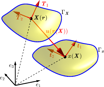
As usual in finite strain theory, we consider an undeformed material configuration and a deformed spatial configuration. These are represented by the -dimensional manifolds and , respectively, which are immersed in a -dimensional space , herein, . The difference is also called codimension of the manifold. We follow the usual notation to relate uppercase letters in variable and operator names with the undeformed configuration and lowercase letters with the deformed one. The displacement field relates the two configurations via
2.2 Parametrized manifolds
For parametrized manifolds, there exists a map from some lower-dimensional reference domain to the undeformed configuration . An important consequence is that local curvilinear coordinate systems result naturally on the manifolds. It is useful to describe the situation separately for cables (one-dimensional manifolds) and membranes (two-dimensional manifolds).
2.2.1 Two-dimensional manifolds
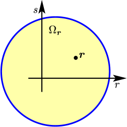
We start with two-dimensional manifolds () in the three-dimensional space () which is relevant for membranes. Let there be a reference domain and a map , see Fig. 1. We label the components and . The Jacobi matrix
has dimensions . One may easily obtain two vectors and from the columns of being tangential to at a mapped point . The Jacobi matrix is also used to compute the first fundamental form and the operator , later needed for defining surface gradients,
| (2.1) |
Next, we consider a displacement field assuming that a point is given which may also be seen as a function when a point is given (and back-projected to the reference domain inverting the map ). We emphasize that in both cases, the displacement field only lives on the manifold . Hence, no classical partial derivatives with respect to may be computed (unless is smoothly extended to some neighborhood of which is not unique and not considered here) so that the only useful gradient of in this context is the surface gradient. For some scalar function , e.g., each displacement component, the surface gradient is
For a vector function , we have the directional surface gradient
| (2.2) |
which is to be distinguished from the covariant surface gradient of a vector field defined in Section 2.5.1.
Let us next consider the map from the undeformed to the deformed configuration which is . The related Jacobi matrix is also called surface deformation gradient,
| (2.3) |
where is a identity matrix.
One may obtain all equivalent quantities in the deformed configuration: The Jacobi-matrix from the reference to the deformed configuration and the tangent vectors , to the deformed configuration at a mapped point based on the Jacobi matrix . Furthermore, the first fundamental form and the operator relating the classical gradient of the reference configuration with the surface gradient of the deformed configuration as .
Based on the pairs of tangent vectors in the undeformed and deformed configuration, one may compute unique normal vectors in each configuration, and . Then, the projectors and are computed as
| (2.4) | |||||
| (2.5) |
The same result is obtained when computing a tangent vector in the tangent plane spanned by and being orthogonal to using Gram Schmidt orthogonalization, , then
analogously for . The projector at some point maps an arbitrary vector in to the tangent space at , hence, . is symmetric, , and idempotent, , which holds analogously for .
Next, we are interested in the stretch of a differential element of the membrane when undergoing the deformation. This is interpreted as an area stretch and defined as
Finally, an operator is introduced which relates surface gradients of the undeformed and the deformed configuration as
| (2.6) |
This result is obtained using and . Note that and are -matrices, hence, not quadratic and the concept of generalized inverses (or pseudo inverses) is needed to obtain Eq. (2.6).
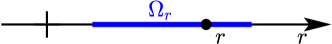
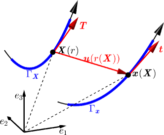
2.2.2 One-dimensional manifolds
Consider some one-dimensional reference domain and a map , , see Fig. 2. This situation applies to cables in two and three dimensions. The Jacobi matrix consists of one column only which implies a tangent vector being tangential to the undeformed configuration at . For the tangent vector in the deformed configuration follows . Most parts of the discussion from Section 2.2.1 apply accordingly. However, the definition of the projectors changes to
| (2.7) | |||||
| (2.8) |
For the stretch of a differential element of the cable, which may be seen as a line stretch, there follows
2.3 Implicit manifolds
Implicit manifolds are implied by one or more level-set functions. Generally speaking, the codimension determines the number of level-set functions required to define a unique geometry of a manifold. For the cases relevant in this work, this means that one level-set function is required for cables in and membranes in which have codimension . For cables in , on the other hand, two level-set functions and are needed. We split the discussion depending on the codimension.
2.3.1 Manifolds with codimension
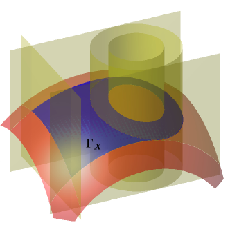
Oriented manifolds with codimension may be defined by one level-set function . Usually, the zero-level set of implies the manifold of interest and there are infinitely many possible implying the same geometry. The signed distance function is a particularly useful concrete example for and often used in practice. It is noteworthy that many level-sets are unbounded in which is not desirable for the definition of mechanical applications. Fortunately, it is easily possible to define bounded manifolds by additional (slave) level-set functions , see [20, 22]. Then, the undeformed configuration is, e.g., given by
| (2.9) |
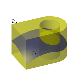
as shown in Fig. 3(a). Even simpler is to associate a domain of definition with , then the bounded manifold results as
| (2.10) |
In this case, the boundaries are the intersections of the zero-level set with the boundary of the domain of definition, see Fig. 3(b). The implicit definition according to Eq. (2.10) is used in the following unless noted otherwise.
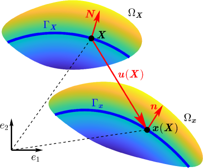
Next, we focus on the situation in large displacement theory as shown in Fig. 4 for this implicit setup. The normal vector of the undeformed configuration is obtained by the gradient of the level-set function,
Let there be a displacement field which lives in the full -dimensional space (instead of only the manifold itself as for parametric manifolds) so that the classical gradient is available. The resulting deformation gradient is
| (2.11) |
which is different from the surface deformation gradient in Eq. (2.3). Based on this, one may compute the normal vector of the deformed configuration at as
which follows by the chain rule. Eqs. (2.4) and (2.5) are used to compute the projectors and , respectively. The surface gradient (with respect to the undeformed configuration) of a scalar function with results as
| (2.12) |
As before, is the classical gradient in the -dimensional space. The situation is analogous for each component of a vector function , so that one obtains for the directional surface gradient
| (2.13) | |||||
| (2.23) |
The surface deformation gradient follows using Eq. (2.3). The stretch of a differential element upon the deformation is
Finally, for the operator relating surface gradients of the undeformed and deformed configuration, one obtains
| (2.24) |
Note that , hence, when using the classical derivatives one obtains .
2.3.2 Manifolds with codimension
The focus is on one-dimensional manifolds in such as cables in the three-dimensional space. As mentioned before, two level-set functions and are needed for the geometry definition,
see Fig. 5. The -dimensional displacement field is given as before with classical derivatives and the related deformation gradient as in Eq. (2.11).
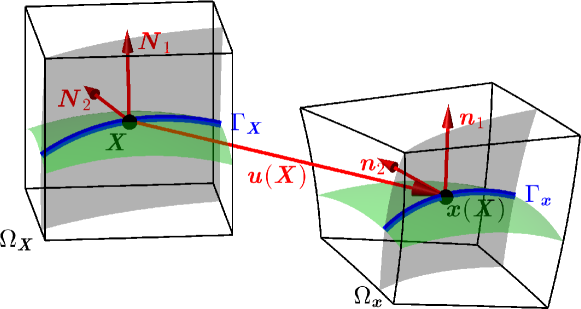
The two normal vectors associated to the deformed and undeformed configuration each, are given for as
One may then compute the unique tangent vectors
The projectors and follow using Eqs. (2.7) and (2.8), respectively. It is noted that the same projector is obtained when using and the orthogonalized normal vector and
analogously for . As before, these projectors are used to determine surface gradients of scalar and vector functions as in Eqs. (2.12) and (2.13). The line stretch is given as
2.4 Similarities and differences in the parametric and implicit descriptions
In this section, purely based on geometric considerations related to the undeformed and deformed situation, a number of useful quantities and operators are given following the concept of the TDC. The situation is summarized in Table 1 for parametric manifolds and in Table 2 for implicit ones. For the mathematical equivalence of these two descriptions and more details, see, e.g., [15]. The order of the rows in the tables is determined by the information available for parametric and implicit manifolds. Thereby, it is made sure that the (geometric and differential) quantities of interest may be computed in this order.
| undeformed config. | ||
|---|---|---|
| deformed config. | ||
| projectors | ||
| line/area stretch | ||
| relation | ||
| undeformed config. | ||
|---|---|---|
| deformed config. | ||
| projectors | ||
| line/area stretch | ||
It was found above that for parametrized manifolds, tangent vectors result naturally as primary quantities through the existence of Jacobi matrices. For problems with codimension , one may then obtain normal vectors as secondary quantities (e.g., by a cross product of tangent vectors), however, for higher codimensions, no unique normal vector exists. For implicit manifolds, the situation is rather the opposite: Here, normal vectors result naturally through the gradients of level-set functions. A unique tangent vector is only applicable for one-dimensional manifolds and may, for example, be computed by a cross product of the normal vectors. This situation is an example of the duality in the parametric and implicit description of manifolds.
2.5 Further definitions
Based on the previous definitions, some additional differential operators are introduced which apply to parametric and implicit manifolds equivalently.
2.5.1 Covariant surface gradient and divergence
The covariant surface gradient of a vector function is based on the projection of the directional one (see Eqs. (2.2) and (2.13) for the parametric and implicit situation, respectively) onto the tangent space. With respect to the undeformed configuration, it is defined as
| (2.25) |
Concerning the surface divergence of vector functions and tensor functions , there holds
| (2.26) | |||||
| (2.30) |
The divergence operator with respect to the deformed configuration follows accordingly as and , respectively.
2.5.2 Conormal vector on the boundary
Unit normal and tangent vectors on manifolds have already been used before and exist with respect to the deformed and undeformed configuration, respectively. For example, the unit normal vector on an undeformed membrane is for all and, after the deformation, for all . It is important to note that, for physical reasons, the manifolds used in this work are bounded. The boundary of the undeformed configuration is labeled and in the deformed situation .
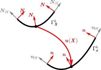
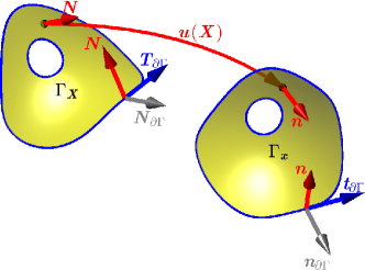
There exists a conormal unit vector along the boundary which is in the tangent plane of the manifold yet normal to . This vector points out of the manifold in the direction which naturally extends the manifold, see Fig. 6. The computation of the conormal vectors is straightforward (often using cross products) and depends on and . In the deformed configuration, the situation is similar for computing for all . In the context of the definition of boundary value problems on manifolds, the conormal vectors play a crucial role for the consideration of boundary conditions as shall be seen in Section 3.1.5.
2.5.3 Divergence theorem on manifolds
To derive the weak form of the governing equations later on, the following divergence theorem on manifolds is needed [12, 14],
| (2.31) |
where is a matrix scalar product. The mean curvature is with being the second fundamental form. For in-plane tensor functions with , the term involving the curvature vanishes and one finds .
3 Mechanical model and governing equations
In Section 2, a number of geometric quantities (such as normal vectors, projectors, area/line stretches etc.) and differential operators related to (surface) gradients are introduced. It was shown how these quantities are obtained for parametrized and implicitly defined manifolds. The focus is now turned to the mechanics and the procedure follows the classical outline, however, it is based on the TDC here. It is emphasized that all tensors considered in the following refer to the parametric as well as implicit situation. These tensors have dimensions (with being the dimension into which the cable or membrane is immersed). A tensor is called “in-plane” or “tangential” to the undeformed configuration if and to the deformed configuration if . An in-plane -tensor has non-zero eigenvalues representing the principal mechanical quantity (with being the dimension of the manifold: for cables, for membranes).
Starting point is the surface deformation gradient at , specified previously in Eq. (2.3). It may also be seen as a geometrical quantity mapping tangent vectors from the undeformed to the deformed configuration. It is also noted that the situation also applies to the “volumetric” case (where are flat shells in two dimensions and are volumetric continua in three dimensions). In this case, as in Eq. (2.11), and for the projectors, . In that sense, the presented mechanical outline below applies to cables, membranes and continua in a unified sense.
3.1 Governing equations in strong form
3.1.1 Strain tensors
Based on the surface deformation gradient, the directional and tangential Cauchy-Green strain tensors are defined as
| /12 | (3.1) | ||||
| (3.2) |
respectively. The Euler-Almansi strain tensors are
| /12 | (3.3) | ||||
| (3.4) |
where is tangential to the deformed configuration . As usual, there holds (which is not true for the tangential versions of these strain tensors).
3.1.2 Stress tensors
Conjugated stress tensors are introduced next and only the tangential versions are considered. Generally speaking, we assume some hyper-elastic material with an elastic energy function and obtain the second Piola-Kirchhoff stress tensor as . For simplicity, only Saint Venant–Kirchhoff solids are considered herein and there follows
with being tangential to . and are the Lamé constants; for cables becomes . On the other hand, the Cauchy stress tensor reads
| (3.6) |
where is a line stretch for cables and an area stretch for membranes when undergoing the displacement, see Section 2. For the volumetric case (), is the volumetric stretch. The Cauchy stress is tangential to the deformed configuration since and , hence The first Piola-Kirchhoff stress tensor is given by
| (3.7) |
and there holds .
3.1.3 Relation of stress and strain tensors
For every point and its mapped counterpart , we have the following equality,
| (3.8) |
where represents the matrix scalar product operator. In this sense the two stress tensors and are conjugated to their related strain tensors and , respectively. It is noted that
which will be important later. Furthermore, the result of these matrix scalar products may also be derived by the non-zero eigenvalues , , , , , of the tangential tensors , , , , respectively. Hence, we obtain
3.1.4 Equilibrium
A crucial aspect of finite strain theory is that equilibrium is to be fulfilled in the deformed configuration which is expressed in strong form as
| (3.9) |
where are body forces. Recall from (2.30) that is the divergence of the Cauchy stress tensor with respect to . Furthermore, we have the identity
| (3.10) |
with being the divergence of the first Piola-Kirchhoff stress tensor from Eq. (3.7) with respect to . In order to transform the derivatives in the divergence operators from the undeformed to the deformed situation, use Eqs. (2.6) and (2.24) for parametric and implicit manifolds, respectively. Due to , the equilibrium in can be stated equivalently to Eq. (3.9) based on quantities in the undeformed configuration as
| (3.11) |
3.1.5 Boundary conditions
The domain of interest is a bounded manifold where the boundary falls into the two non-overlapping parts and , which holds in the deformed and undeformed configuration and , respectively. Hence, the boundary conditions in the deformed configuration are
| (3.12) | ||||
| (3.13) |
where are prescribed displacements and are tractions (force per area for , force per length for or a single force for ). Note that for ropes and membranes, must be in the tangent space of the deformed manifold in order to satisfy the equilibrium due to the absence of bending stresses or transverse shear stresses. The equivalent boundary conditions formulated in the undeformed configuration are
| (3.14) | ||||
| (3.15) |
where and have similar interpretations as before. The relation between and is , where
Further information about boundary conditions for ropes and membranes are given in [8].
With the boundary conditions above, the complete second-order boundary value problem (BVP) is defined in the deformed and undeformed configuration. The obtained BVP in the frame of the TDC is valid for explicitly and implicitly defined manifolds and does not rely on curvilinear coordinates implied by a parametrization, which are typically used in classical approaches, see, e.g., [8, 10]. Therefore, the proposed formulation of ropes and membranes based on the TDC is more general compared to the classical theory.
3.2 Governing equations in weak form
For stating the governing equations in weak form, the following test and trial function spaces are introduced
| (3.16) | ||||
| (3.17) |
where is the Sobolev space of functions with square integrable first derivatives. The task is to find such that for all , there holds
| (3.18) |
where
The integrals in Eq. (3.18) are one-, two-, or three-dimensional for cables, membranes and continua, respectively. The multiplication with ensures that the units of the integration are always consistent. Hence, it is possible to naturally consider situations where cables, membranes and continua are coupled in one setup by simply adding up the corresponding integrals as in Eq. (3.18) for each structure. In order to obtain Eq. (3.18), we applied the usual procedure for converting the strong form to a weak form: Multiply Eq. (3.11) with test functions, integrate over the domain , and apply the divergence theorem from Eq. (2.31). It is noteworthy that the curvature term from Eq. (2.31) vanishes also for cables and membranes due to .
The weak form stated above is related to energy minimization in the sense that
where is the variational operator.
3.2.1 Energy relation
An immediate consequence of Eq. (3.8) is that one may obtain the same stored potential energy of the deformed body by integrating over the undeformed or deformed configuration as follows
| (3.19) | |||||
| (3.20) |
4 Discretization and numerical methods
In order to solve the boundary value problem, i.e., to approximate the sought displacements, one may use two fundamentally different approaches. Possibly the more intuitive one is to discretize the cable(s) or membrane(s) by curved (-dimensional) line or surface elements, respectively. Then, each element results from an (often isoparametric) map of some reference element so that this approach is naturally linked to the parametric description of manifolds as discussed in Section 2.2. This is the classical approach labeled Surface FEM herein. An alternative is to use a (-dimensional) background mesh for the approximation of the weak form. That is, higher-dimensional shape functions (than the dimension of the manifold) are used and evaluated on the trace of the manifold only. This approach is called Trace FEM or Cut FEM. It is naturally related to an implicit manifold description as discussed in Section 2.3.
It is important to note that the classical definition of finite strain theory based on curvilinear coordinates does not cover the latter approach. This is another reason why the presented formulation based on the TDC is more general as it supports both, the Surface and Trace FEM. For the discussion below, we assume the manifold case, hence, . With , the situation results in the standard FEM which is not further outlined here.
4.1 Surface FEM
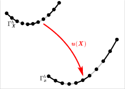
Starting point is the discretization of the undeformed cable () or membrane () by a line or surface mesh, respectively. Herein, we use higher-order -dimensional Lagrange elements with equally spaced nodes in the reference element. The nodal coordinates in the undeformed configuration are labeled with and being the number of nodes in the mesh, see Fig. 7. The resulting shape functions span a -continuous finite element space as
| (4.1) |
are obtained by isoparametric mappings from the -dimensional reference element to the physical elements in dimensions. Based on Eq. (4.1), the following discrete test and trial function spaces are introduced
| (4.2) | ||||
| (4.3) |
The discrete weak form of Eq. (3.18) reads as follows: Given Lamé constants , body forces on , tractions on , find the displacement field such that for all test functions there holds in
| (4.4) |
The sought discrete displacement field is obtained solving a non-linear system of equations for the nodal values (degrees of freedom) as usual in the context of finite strain theory.
4.2 Trace FEM
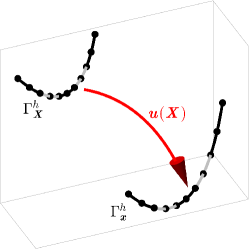
Let there be a -dimensional background mesh into which the manifold is completely immersed. Only those elements and corresponding nodes are considered that are cut by the manifold, see Fig. 8. They may be labeled “active” elements and nodes, all others are neglected. The shape functions of the active nodes are constructed by (often isoparametric) mappings from a -dimensional reference element, but the shape functions are only evaluated on the -dimensional manifold.
The Trace FEM is a fictitious domain method (FDM) for PDEs on manifolds [33, 32, 25, 23]. As in any FDM, there is no boundary-conforming mesh but a background mesh, herein further complicated by the fact that background mesh and manifold have different dimensions. In general, the following issues have to be properly addressed:
-
1.
Integration points have to be defined for the integration of the weak form of the governing equations—only at these points, shape functions are evaluated. This requires the identification of the zero-level set of some level-set function within each active background element, see Fig. 9. The situation may be further complicated, when the boundary of the manifold is within the background element, which may be defined by additional slave level-set functions as mentioned in Section 2.3. The placement of integration points is an important and challenging task, in particular with higher-order accuracy. For an overview, we refer to the references [18, 34, 19, 21]. It is useful to evaluate given level-set functions at the active nodes and interpolate them in-between. The identification of the zero-level sets and placement of integration points may then be achieved in the -dimensional reference element which simplifies the evaluation of shape functions in the background elements. Of course, the interpolated zero-level set is only a (higher-order) approximation of the exact manifolds and and labeled and , respectively. In the Trace FEM context, and may be seen as integration cells, see Fig. 9(b), to define integration points, they do not imply shape functions.
-
2.
The treatment of boundary conditions is a challenging task in FDMs as it is impossible to directly prescribe values of the nodes in the active background elements. The additional constraints may, in principle, be enforced using penalty methods, Lagrange multiplier methods, or Nitsche’s method. The latter has been developed to be a standard choice in FDMs because the equations are formulated in a consistent way without needing additional degrees of freedom [31]. In the standard (symmetric) form of the Nitsche’s method, stabilization parameters are required. In the simplest case, these parameters may be set to a fixed user-defined number [6, 26], however, for background elements which are cut by a tiny fraction of the manifold, resulting in small supports of the shape functions, this may lead to unsatisfactory results. An alternative is to compute the stabilization parameters based on global or element-wise generalized eigenvalue problems [16, 40]. However, for the awkward cut situations, this may result in unbounded values resulting in similar problems known for penalty methods [11]. Therefore, we prefer the non-symmetric Nitsche’s method herein with the main advantage that an additional stabilization is not required for imposing boundary conditions [3, 41].
-
3.
Stabilization is still necessary when applying FDMs in the context of PDEs on manifolds to ensure the regularity of the resulting system of equations. This may be traced back to two sources: One is found in the shape functions with small supports and the other in the fact that the approximated displacement field on the manifold may not necessarily be represented by a unique set of nodal values in the background mesh. That is, the background shape functions restricted to the manifold build a frame but not necessarily a basis [23, 38, 32]. Fortunately, different stabilization approaches exist to cure both issues and we refer to the overview given in [32] for the Trace FEM. Herein, we use the “normal derivative volume stabilization”, introduced for scalar-valued problems in [24, 7] and in [25] for vector-valued problems. This stabilization technique enables higher-order accurate results, does not change the sparsity pattern of the stiffness matrix, and only first derivatives are needed.
With these comments made, we are ready to define the discrete weak form for the Trace FEM. Let be the background mesh into which the undeformed configuration is immersed, only active elements and nodes are present in . The resulting shape functions span a -continuous finite element space on the manifold as
| (4.5) |
Based on Eq. (4.5), the following discrete trace test and trial function spaces are introduced
| (4.6) | ||||
| (4.7) |
For the Trace FEM, the discrete weak form of Eq. (3.18) is: Given Lamé constants , body forces on , tractions on , and stabilization parameter , find the displacement field such that for all test functions there holds in
| (4.8) | |||
In comparison to Eq. (4.4), additional terms occur in the discrete weak form due to the weak enforcement of essential boundary conditions with Nitsche’s method and the stabilization. The sought discrete displacement field is obtained solving a non-linear system of equations for the nodal values (degrees of freedom).
Note that the stabilization term is the only term which is not evaluated on the manifold but in the volumetric background mesh (using standard Gauss integration). Therefore, one has to extend the normal vector from the undeformed manifold to the neighborhood, resulting in for all . This is particularly simple for implicitly defined manifolds, e.g., using for all . Furthermore, in the stabilization term, the classical gradient operator is used instead of the surface operators used in the other terms. In [24], it is recommended that the stabilization parameter should be chosen in the range , where is the element size in the active background mesh.
A remark is added concerning slip supports because the above mentioned weak form rather expects that all displacement components are prescribed through along the Dirichlet boundary . In the Nitsche’s method, displacement constraints in selected, arbitrary unit directions with magnitude may be prescribed by replacing the corresponding terms in Eq. (4.8) with
| (4.9) | ||||
5 Numerical results
A number of test cases for ropes and membranes in two and three dimensions are considered in this section. The numerical results focus on the convergence rates for two different types of errors. The “energy error” compares the approximated stored elastic energy with the analytical one,
| (5.1) |
with computed based on Eq. (3.19). The analytical energy may also be computed by an overkill approximation, i.e., based on an extremely fine mesh with higher-order elements. Provided that geometry and boundary conditions allow for sufficiently smooth solutions, the expected convergence rates in this error norm are with being the order of the elements.
The “residual error” integrates the error in the equilibrium as stated in Eq. (3.9), that is,
| (5.2) |
This error obviously vanishes for the analytical solution. It is important to note that the integrand in (5.2) involves second-order derivatives. Therefore, the integral must not be carried out over the whole (discretized) domain but integrated element by element as indicated by the summation. That is, element boundaries, where already the first derivatives of the -continuous shape functions feature jumps, are neglected in computing . Due to the presence of second-order derivatives, the expected convergence rates are which also indicates that higher-order elements are crucial for convergence in .
5.1 Membrane with given deformation
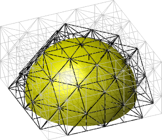
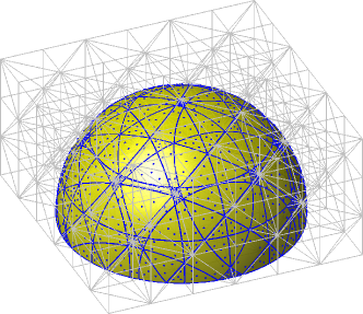
In the first test case, a membrane in the shape of a half sphere with radius undergoes a prescribed displacement and the stored elastic energy is computed from the viewpoint of the Surface FEM and the Trace FEM. That is, in the Surface FEM, surface meshes with different resolutions and element orders are generated. See Fig. 7(c) for some example mesh composed by quadratic elements. The displacements
| (5.3) |
are evaluated at the nodes and interpolated based on the shape functions implied by the surface meshes, yielding ; see Fig. 7(c) for the resulting deformed membrane. Then, the elastic energy of the deformed configuration is computed with Eq. (3.19).
For the Trace FEM viewpoint, background meshes of different resolutions and orders are generated in and the geometry is defined based on the level-set function . See Fig. 8(c) for a sketch of the situation using quadratic background elements. Then, the (active) nodes of the background mesh are deformed by the given displacement field (5.3), yielding based on the shape functions implied by the background meshes. This displacement field living in the whole background mesh is only evaluated on the membrane surface in order to compute the stored energy according to the Trace FEM.
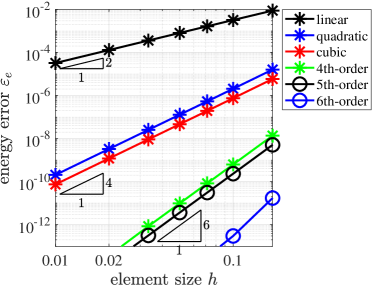
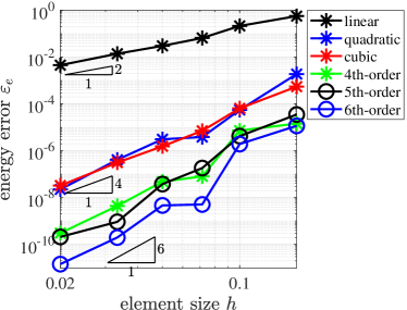
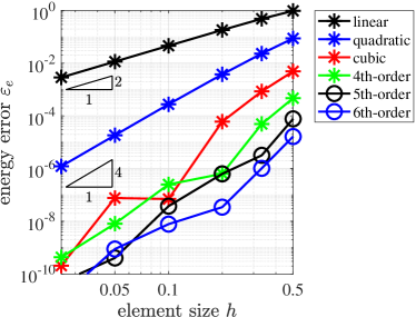
We set the Lamé constants to and . The resulting energy is given by the value . In Fig. 10, the convergence results for the various meshes are shown for the Surface and the Trace FEM. It is seen that in both cases optimal convergence results are achieved. The energy error converges one order higher than expected for even element orders. In the Trace FEM, the convergence curves are less smooth than in the Surface FEM because the approximation spaces are not nested upon refinement; this is well-known for results obtained with FDMs in general.
It is thus seen that the Surface FEM as well as the Trace FEM have the potential to achieve optimal results. For all other test cases below, we shall now obtain the discrete displacement fields based on solving the non-linear systems of equations resulting from the weak forms given in Section 4.
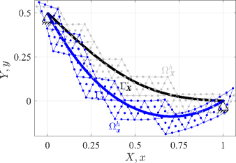
5.2 Rope with Surface and Trace FEM
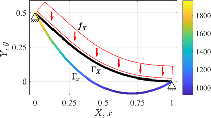
The second test case considers a rope in two dimensions as shown in Fig. 11. The cross section of the rope is , Young’s modulus is , and the Lamé constants are and . The left support is located at and the right at . The geometry may be given in parametric form for as
Alternatively, the same geometry may be implied by the level-set function
The structure is loaded by its own weight with for all . The deformed rope is illustrated in Fig. 11(a) where the color information indicates the principal Cauchy stress in the rope. The stored elastic energy is and the length of the rope is increased by a factor of due to the deformation.
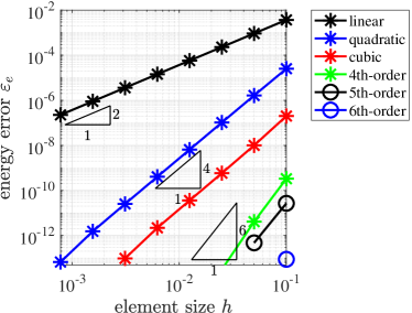
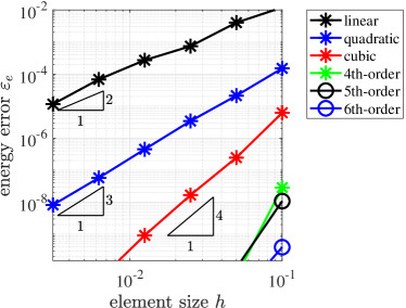
The displacements are computed with the Surface and Trace FEM, respectively. For the Trace FEM, the stabilization parameter in Eq. (4.8) is set to . The mesh resolutions and orders are systematically varied and convergence results are seen in Fig. 12. Figs. 12(a) and (b) show the error in the elastic energy and Figs. 12(c) and (d) the residual error . Of course, for some given element length , the use of (curved) line meshes in the Surface FEM results in considerably less degrees of freedom than using background meshes in the Trace FEM. Therefore, the convergence studies for the Surface FEM are realized for up to elements whereas the background meshes in the Trace FEM feature up to elements (of which only those cut by the rope are active and, hence, taken into account for the simulation). It is apparent from the convergence results in Fig. 12 that optimal higher-order convergence rates are achieved. It is noteworthy that the Surface FEM with even element orders converges one order higher than expected in , whereas this is not the case for the Trace FEM. This can already be traced back to the accuracy in the numerical integration: Simply integrating the length of the rope using the Surface or Trace FEM viewpoint shows that an extra order in the accuracy is achieved with the Surface FEM for even element orders. For the convergence results in , results for linear meshes are omitted because second order derivatives are needed for this error measure, see Eq. (5.2). In this error norm, Surface and Trace FEM converge optimally with .
5.3 Membranes with Surface FEM
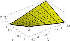
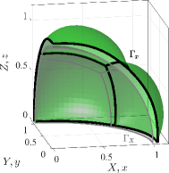
For the next test case, the deformation of membranes is approximated with the Surface FEM. Two different undeformed configurations are considered which result from a map of a unit circle for map A and of a unit square for map B. The undeformed configurations are given by the parametrizations
| (5.4) |
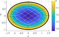
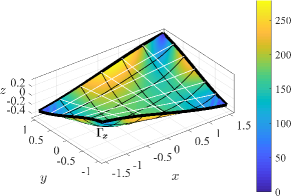
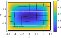
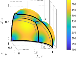
where is a scaling parameter in vertical direction. The resulting configurations for map A and B are illustrated in Figs. 13(a) and (d) for , respectively. An important difference is that the boundary is smooth for map A but involves corners for map B, later resulting in different convergence behaviors. The thickness of the membrane is , Young’s modulus is and Poisson ratio , which is easily converted into the Lamé parameters. The loading is gravity acting on the membrane surface with for all . The whole boundary is treated as a Dirichlet boundary with prescribed zero-displacements. The deformed configurations are displayed in Figs. 13(b) and (e) with computed von-Mises stresses based on the Cauchy stress tensor. The vertical displacement field is given in Fig. 13(c) and (f) for the two maps in top view, respectively.

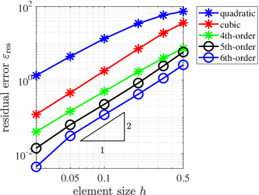
Convergence results are given in Fig. 14. For map A, where the boundary is smooth, optimal convergence rates are found in the energy error and residual error . For map B, where corners are present in the membrane geometry, it is seen that the convergence rates are bounded. Only linear and quadratic elements converge optimally in , higher orders improve the error level, however, not the convergence rates. It is thus confirmed that corners in membranes have the potential to reduce the convergence rates.
5.4 Coupled ropes and membranes
It was mentioned several times that the proposed framework allows for a unified treatment of ropes and membranes (and even continua). This shall be confirmed with this last test case where cables and membranes are coupled. The situation may be described as an inflated ball with embedded reinforcement cables, see Fig. 15(a). The original radius of the ball is and the inner pressure is . This pressure converts to a loading of which depends on the normal vector of the deformed configuration, hence on the displacements , thereby adding a new source of non-linearity which has to be properly considered in the Newton-Raphson loop. The membrane is defined by the parameters , and . The cables which are on the gray planes in Fig. 15(a) feature a Young’s modulus of and a cross section of . All other cables have a Young’s modulus of . For the modeling, only one eighth of the initial sphere is considered, see Fig. 15(b) for the deformed and undeformed situations. Symmetry boundary conditions are applied. The resulting von-Mises stresses in the membrane are shown in Fig. 15(c). The elastic energy stored in the membrane and ropes is given as .
The convergence results are seen in Fig. 16 for the energy error and residual error . It is again seen that the convergence rates in are optimal for linear and quadratic elements. Higher orders achieve better results, however, do not improve the convergence rates. The reason for the bounded convergence rates is found in the stress concentrations where the embedded cables meet, see Fig. 15(c).
6 Conclusions
The modeling of ropes and membranes leads to partial differential equations on manifolds. Herein, a framework is proposed which unifies the mechanical modeling of ropes and membranes undergoing large displacements and, furthermore, applies to parametric and implicit definitions of manifolds. The fundamental ingredient is the use of Tangential Differential Calculus (TDC) for the definition of geometric and differential quantities on the manifolds. The proposed TDC-based formulation is more general than the classical parametric formulation based on curvilinear coordinates because it allows for two different numerical approaches, the Surface and the Trace FEM. The classical approach is restricted to the Surface FEM and cannot handle manifolds which are defined implicitly (unless discretized by a surface mesh).
Even in the classical setting using the Surface FEM with parametric formulations, the new TDC-based formulation leads to a significantly different implementation, however, ultimately achieving the same results (as expected). The advantage of the TDC-based formulation is that it also applies immediately to implicit definitions and the Trace FEM. More technically speaking, we have one element integration routine which applies to ropes and membranes (and even continua) no matter whether we are using the Surface FEM or the Trace FEM. Of course, in the Trace FEM, additional terms have to be considered for the stabilization.
The numerical results consider various test cases with ropes and membranes in two and three dimensions. The Surface and Trace FEM with higher-order elements are used successfully, achieving higher-order convergence rates. It is confirmed that the smoothness of the geometry and the coupling of ropes and membranes has an important influence on the convergence behavior.
References
- [1] Ahmad, S.; Irons, B.M.; Zienkiewicz, O.C.: Analysis of thick and thin shell structures by curved finite elements. Internat. J. Numer. Methods Engrg., 2, 419–451, 1970.
- [2] Bischoff, M.; Ramm, E.; Irslinger., J.: Models and Finite Elements for Thin-Walled Structures. Encyclopedia of Computational Mechanics Second Edition (eds E. Stein, R. Borst and T. J. Hughes), John Wiley & Sons, Chichester, 2017.
- [3] Burman, E.: A penalty-free nonsymmetric Nitsche-type method for the weak imposition of boundary conditions. SIAM J. Numer. Anal., 50, 1959–1981, 2012.
- [4] Burman, E.; Claus, S.; Hansbo, P.; Larson, M.G.; Massing, A.: CutFEM: Discretizing geometry and partial differential equations. Internat. J. Numer. Methods Engrg., 104, 472–501, 2015.
- [5] Burman, E.; Hansbo, P.: Fictitious domain finite element methods using cut elements: I. A stabilized Lagrange multiplier method. Comp. Methods Appl. Mech. Engrg., 199, 2680–2686, 2010.
- [6] Burman, E.; Hansbo, P.: Fictitious domain finite element methods using cut elements: II. A stabilized Nitsche method. Applied Numerical Mathematics, 62, 328–341, 2012.
- [7] Burman, E.; Hansbo, P.; Larson, M.G.; Massing, A.: Cut Finite Element Methods for Partial Differential Equations on Embedded Manifolds of Arbitrary Codimensions. ArXiv e-prints, 2016.
- [8] Calladine, C. R.: Theory of Shell Structures. Cambridge University Press, Cambridge, 1983.
- [9] Chapelle, D.; Bathe, K.J.: The Finite Element Analysis of Shells – Fundamentals. Computational Fluid and Solid Mechanics. Springer, Berlin, 2011.
- [10] Ciarlet, P.G.: Mathematical Elasticity, III: Theory of Shells. Elsevier, Amsterdam, 1997.
- [11] de Prenter, F.; Lehrenfeld, C.; Massing, A.: A note on the stability parameter in Nitsche’s method for unfitted boundary value problems. Comp. Methods Appl. Mech. Engrg., 75, 4322–4336, 2018.
- [12] Delfour, M.C.; Zolésio, J.P.: Tangential Differential Equations for Dynamical Thin-Shallow Shells. Journal of Differential Equations, 128, 125–167, 1996.
- [13] Delfour, M.C.; Zolésio, J.P.: Differential equations for linear shells comparison between intrinsic and classical. Advances in Mathematical Sciences: CRM’s 25 Years (Montreal, PQ, 1994), CRM Proc. Lecture Notes, 1997.
- [14] Delfour, M.C.; Zolésio, J.P.: Shapes and geometries—Metrics, Analysis, Differential Calculus, and Optimization. SIAM, Philadelphia, PA, 2011.
- [15] Dziuk, G.; Elliott, C.M.: Finite element methods for surface PDEs. Acta Numerica, 22, 289–396, 2013.
- [16] Fernández-Méndez, S.; Huerta, A.: Imposing essential boundary conditions in mesh-free methods. Comp. Methods Appl. Mech. Engrg., 193, 1257–1275, 2004.
- [17] Fries, T.P.: Higher-order surface FEM for incompressible Navier-Stokes flows on manifolds. Int. J. Numer. Methods Fluids, 88, 55–78, 2018.
- [18] Fries, T.P.; Omerović, S.: Higher-order accurate integration of implicit geometries. Internat. J. Numer. Methods Engrg., 106, 323–371, 2016.
- [19] Fries, T.P.; Omerović, S.; Schöllhammer, D.; Steidl, J.: Higher-order meshing of implicit geometries—part I: Integration and interpolation in cut elements. Comp. Methods Appl. Mech. Engrg., 313, 759–784, 2017.
- [20] Fries, T.P.; Omerović, S.; Schöllhammer, D.; Steidl, J.: Higher-order meshing of implicit geometries—part I: Integration and interpolation in cut elements. arXiv: 1706.00578, 2017.
- [21] Fries, T.P.; Schöllhammer, D.: Higher-order meshing of implicit geometries—part II: Approximations on manifolds. Comp. Methods Appl. Mech. Engrg., 326, 270–297, 2017.
- [22] Fries, T.P.; Schöllhammer, D.: Higher-order meshing of implicit geometries—part II: Approximations on manifolds. arXiv: 1706.00840, 2017.
- [23] Grande, J.; Lehrenfeld, C.; Reusken, A.: Analysis of a high-order trace finite element method for PDEs on level set surfaces. SIAM J. Numer. Anal., 56, 228–255, 2018.
- [24] Grande, J.; Reusken, A.: A Higher Order Finite Element Method for Partial Differential Equations on Surfaces. SIAM J. Numer. Anal., 54, 388–414, 2016.
- [25] Gross, S.; Jankuhn, T.; Olshanskii, M.A.; Reusken, A.: A trace finite element method for vector-laplacians on surfaces. SIAM J. Numer. Anal., 56, 2406–2429, 2018.
- [26] Hansbo, A.; Hansbo, P.: An unfitted finite element method, based on Nitsche’s method, for elliptic interface problems. Comp. Methods Appl. Mech. Engrg., 191, 5537–5552, 2002.
- [27] Hansbo, P.; Larson, M.G; Larsson, F.: Tangential differential calculus and the finite element modeling of a large deformation elastic membrane problem. Comput. Mech., 56, 87–95, 2015.
- [28] Ibrahimbegović, A.; Gruttmann, F.: A consistent finite element formulation of nonlinear membrane shell theory with particular reference to elastic rubberlike material. Finite Elem. Anal. Des., 13, 75–86, 1993.
- [29] Jankuhn, T.; Olshanskii, M.A.; Reusken, A.: Incompressible fluid problems on embedded surfaces: Modeling and variational formulations. arXiv:1702.02989, 2017.
- [30] Monteiro, E.; He, Q.C.; Yvonnet, J.: Hyperelastic large deformations of two-phase composites with membrane-type interface. Int. J. Engrg. Sci., 49, 985–1000, 2011.
- [31] Nitsche, J.A.: Über ein Variationsprinzip zur Lösung von Dirichlet-Problemen bei Verwendung von Teilräumen, die keinen Randbedingungen unterworfen sind. Abhandlungen aus dem Mathematischen Seminar der Universität Hamburg, Vol. 36, Springer, Berlin, 9–15, 1971.
- [32] Olshanskii, M.A.; Reusken, A.: Trace finite element methods for PDEs on surfaces. Lecture Notes in Computational Science and Engineering, 121, 211–258, 2017.
- [33] Olshanskii, M.A.; Reusken, A.; Grande, J.: A finite element method for elliptic equations on surfaces. SIAM J. Numer. Anal., 47, 3339–3358, 2009.
- [34] Omerović, S.; Fries, T.P.: Conformal higher-order remeshing schemes for implicitly defined interface problems. Internat. J. Numer. Methods Engrg., 109, 763–789, 2017.
- [35] Osher, S.; Fedkiw, R.P.: Level set methods: an overview and some recent results. J. Comput. Phys., 169, 463–502, 2001.
- [36] Osher, S.; Fedkiw, R.P.: Level Set Methods and Dynamic Implicit Surfaces. Springer, Berlin, 2003.
- [37] Pimenta, P.M.; Campello, E.M.B.: Shell curvature as an initial deformation: A geometrically exact finite element approach. Internat. J. Numer. Methods Engrg., 78, 1094–1112, 2009.
- [38] Reusken, A.: Analysis of trace finite element methods for surface partial differential equations. IMA J Numer Anal, 35, 1568–1590, 2014.
- [39] Reusken, A.: Analysis of trace finite element methods for surface partial differential equations. IMA J Numer Anal, 35, 1568–1590, 2015.
- [40] Ruess, M.; Schillinger, D.; Bazilevs, Y.; Varduhn, V.; Rank, E.: Weakly enforced essential boundary conditions for NURBS-embedded and trimmed NURBS geometries on the basis of the finite cell method. Internat. J. Numer. Methods Engrg., 95, 811–846, 2013.
- [41] Schillinger, D.; Harari, I.; Hsu, M.C.; Kamensky, D.; Stoter, S.K.F.; Yu, Y.; Zhao, Y.: The non-symmetric Nitsche method for the parameter-free imposition of weak boundary and coupling conditions in immersed finite elements. Comp. Methods Appl. Mech. Engrg., 309, 625–652, 2016.
- [42] Schöllhammer, D.; Fries, T.P.: Classical shell analysis in view of Tangential Differential Calculus. In Proceedings of the 6th European Congress on Computational Mechanics (ECCM VI). (Oñate, E.; Oliver, X.; Huerta, A.; Huerta, A., Eds.), Glasgow, UK, 2018.
- [43] Schöllhammer, D.; Fries, T.P.: Kirchhoff-Love shell theory based on Tangential Differential Calculus. Proceedings in Applied Mathematics and Mechanics, Vol. submitted, John Wiley & Sons, Chichester, 2018.
- [44] Schöllhammer, D.; Fries, T.P.: Kirchhoff-Love shell theory based on tangential differential calculus. Comput. Mech., 64, 113–131, 2019.
- [45] Schöllhammer, D.; Fries, T.P.: Reissner-Mindlin shell theory based on tangential differential calculus. Comp. Methods Appl. Mech. Engrg., 352, 172–188, 2019.
- [46] Sethian, J.A.: Level Set Methods and Fast Marching Methods. Cambridge University Press, Cambridge, 2 edition, 1999.
- [47] Simo, J.C.; Fox, D.D.; Rifai, M.S.: On a stress resultant geometrically exact shell model. Part II: The linear theory; Computational aspects. Comp. Methods Appl. Mech. Engrg., 73, 53–92, 1989.