LTL Model Checking of Self Modifying Code

Abstract

Self modifying code is code that can modify its own instructions during the execution of the program. It is extensively used by malware writers to obfuscate their malicious code. Thus, analysing self modifying code is nowadays a big challenge. In this paper, we consider the LTL model-checking problem of self modifying code. We model such programs using self-modifying pushdown systems (SM-PDS), an extension of pushdown systems that can modify its own set of transitions during execution. We reduce the LTL model-checking problem to the emptiness problem of self-modifying Büchi pushdown systems (SM-BPDS). We implemented our techniques in a tool that we successfully applied for the detection of several self-modifying malware. Our tool was also able to detect several malwares that well-known antiviruses such as BitDefender, Kinsoft, Avira, eScan, Kaspersky, Qihoo-360, Baidu, Avast, and Symantec failed to detect.

1 Introduction

Binary code presents several complex aspects that cannot be encountred in source code. One of these aspects is self-modifying code, i.e., code that can modify its own instructions during the execution of the program. Self-modifying code makes reverse code engineering harder. Thus, it is extensively used to protect software intellectual property. It is also heavily used by malware writers in order to make their malwares hard to analyse and detect by static analysers and anti-viruses. Thus, it is crucial to be able to analyse self-modifying code.

There are several kinds of self-modifying code. In this work, we consider self-modifying code caused by self-modifying instructions. These kind of instructions treat code as data. This allows them to read and write into code, leading to self-modifying instructions. These self-modifying instructions are usually mov instructions, since mov allows to access memory and read and write into it.

Let us consider the example shown in Figure1. For simplicity, the addresses’ length is assumed to be 1 byte. In the right box, we give, respectively, the binary code, the addresses of the different instructions, and the corresponding assembly code, obtained by translating syntactically the binary code at each address. For example, 0c is the binary code of the jump jmp. Thus, 0c 02 is translated to jmp 0x2 (jump to address 0x2). The second line is translated to push 0x9, since ff is the binary code of the instruction push. The third instruction mov 0x2 0xc will replace the first byte at address 0x2 by 0xc. Thus, at address 0x2, ff 09 is replaced by 0c 09. This means the instruction push 0x9 is replaced by the jump instruction jmp 0x9 (jump to address 0x9), etc. Therefore, this code is self-modifying: the mov instruction was able to modify the instructions of the program via its ability to read and write the memory. If we study this code without looking at the semantics of the self-modifying instructions, we will extract from it the Control Flow Graph CFG a that is in the left of the figure, and we will reach the conclusion that the call to the API function CopyFileA at address 0x9 cannot be made. However, you can see that the correct CFG is the one on the right hand side CFG b, where the call to the API function CopyFileA at address 0x9 can be reached. Thus, it is very important to be able to take into account the semantics of the self-modifying instructions in binary code.

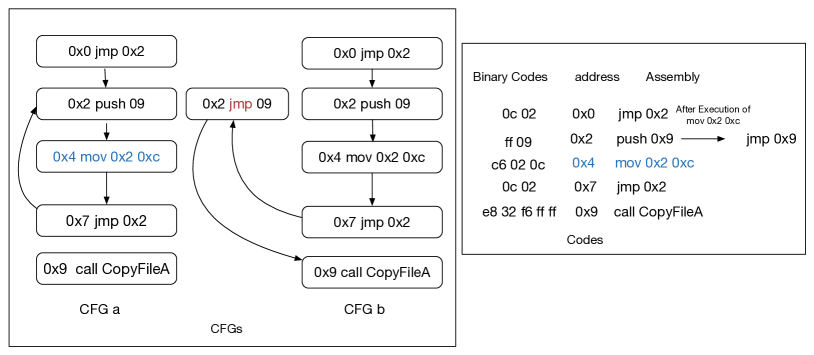
Figure 1: An Example of a Self-modifying Code

In this paper, we consider the LTL model-checking problem of self-modifying code. To this aim, we use Self-Modifying Pushdown Systems (SM-PDSs) [29] to model self-modifying code. Indeed, SM-PDSs were shown in [29] to be an adequate model for self-modifying code since they allow to mimic the program’s stack while taking into account the self-modifying semantics of the transitions. This is very important for binary code analysis and malware detection, since malwares are based on calls to API functions of the operating system. Thus, antiviruses check the API calls to determine whether a program is malicious or not. Therefore, to evade from these antiviruses, malware writers try to hide the API calls they make by replacing calls by push and jump instructions. Thus, to be able to analyse such malwares, it is crucial to be able to analyse the program’s stack. Hence the need to a model like pushdown systems and self-modifying pushdown systems for this purpose, since they allow to mimic the program’s stack.

Intuitively, a SM-PDS is a pushdown system (PDS) with self-modifying rules, i.e., with rules that allow to modify the current set of transitions during execution. This model was introduced in [29] in order to represent self-modifying code. In [29], the authors have proposed algrithms to compute finite automata that accept the forward and backward reachability sets of SM-PDSs. In this work, we tackle the problem of LTL model-checking of SM-PDSs. Since SM-PDSs are equivalent to PDSs [29], one possible approach for LTL model checking of SM-PDS is to translate the SM-PDS to a standard PDS and then run the LTL model checking algorithm on the equivalent PDS [2, 10]. But translation from a SM-PDS to a standard PDS is exponential. Thus, performing the LTL model checking on the equivalent PDS is not efficient.

To overcome this limitation, we propose a direct LTL model checking algorithm for SM-PDSs. Our algorithm is based on reducing the LTL model checking problem to the emptiness problem of Self Modifying Büchi Pushdown Systems (SM-BPDS). Intuitively, we obtain this SM-BPDS by taking the product of the SM-PDS with a Büchi automaton accepting an LTL formula $\varphi$. Then, we solve the emptiness problem of an SM-BPDS by computing its repeating heads. This computation is based on computing labelled $pre^{*}$ configurations by applying a saturation procedure on labelled finite automata.

We implemented our algorithm in a tool. Our experiments show that our direct techniques are much more efficient than translating the SM-PDS to an equivalent PDS and then applying the standard LTL model checking for PDSs [2, 10]. Moreover, we successfully applied our tool to the analysis of 892 self-modifying malwares. Our tool was also able to detect several self-modifying malwares that well-known antiviruses like BitDefender, Kinsoft, Avira, eScan, Kaspersky, Qihoo-360, Baidu, Avast, and Symantec were not able to detect.

Related Work. Model checking and static analysis approaches have been widely used to analyze binary programs, for instance, in [9, 5, 23, 11, 3]. Temporal Logics were chosen to describe malicious behaviors in [20, 11, 3, 4, 8]. However, these works cannot deal with self-modifying code.

POMMADE [3, 4] is a malware detector based on LTL and CTL model-checking of PDSs. STAMAD [15, 16, 14] is a malware detector based on PDSs and machine learning. However, POMMADE and STAMAD cannot deal with self-modifying code.

Cai et al. [7] use local reasoning and separation logic to describe self-modifying code and treat program code uniformly as regular data structure. However, [7] requires programs to be manually annotated with invariants. In [26], the authors propose a formal semantics for self-modifying codes, and use that to represent self-unpacking code. This work only deals with packing and unpacking behaviours. Bonfante et al. [6] provide an operational semantics for self-modifying programs and show that they can be constructively rewritten to a non-modifying program. However, all these specifications [6, 7, 26] are too abstract to be used in practice.

In [1], the authors propose a new representation of self-modifying code named State Enhanced-Control Flow Graph (SE-CFG). SE-CFG extends standard control flow graphs with a new data structure, keeping track of the possible states programs can reach, and with edges that can be conditional on the state of the target memory location. It is not easy to analyse a binary program only using its SE-CFG, especially that this representation does not allow to take into account the stack of the program.

[24] propose abstract interpretation techniques to compute an over-approximation of the set of reachable states of a self-modifying program, where for each control point of the program, an over-approximation of the memory state at this control point is provided. [18] combine static and dynamic analysis techniques to analyse self-modifying programs. Unlike our approach, these techniques [24, 18] cannot handle the program’s stack.

Unpacking binary code is also considered in [13, 17, 22, 26]. These works do not consider self-modifying mov instructions.

Outline. The rest of the paper is structured as follows: Section 2 recalls the definition of Self Modifying pushdown systems. LTL model checking and SM-BPDSs are defined in Section 3. Section 4 solves the emptiness problem of SM-BPDS. Finally, the experiments are reported in Section 5.

2 Self Modifying Pushdown Systems

2.1 Definition

We recall in this section the definition of Self-modifying Pushdown Systems [29].

Definition 1.

A Self-modifying Pushdown System (SM-PDS) is a tuple $\mathcal{P}=(P,\Gamma,\Delta,\Delta_{c})$, where $P$ is a finite set of control points, $\Gamma$ is a finite set of stack symbols, $\Delta\subseteq(P\times\Gamma)\times(P\times\Gamma^{*})$ is a finite set of transition rules, and $\Delta_{c}\in P\times\Delta\times\Delta\times P$ is a finite set of modifying transition rules. If $((p,\gamma),(p^{\prime},w))\in\Delta$, we also write $\langle p,\gamma\rangle\hookrightarrow\langle p^{\prime},w\rangle\in\Delta$. If $(p,r_{1},r_{2},p^{\prime})\in\Delta_{c}$, we also write $p\stackrel{{\scriptstyle(r_{1},r_{2})}}{{\lhook\joinrel\relbar\joinrel\relbar\joinrel\relbar\joinrel\relbar\joinrel\rightarrow}}p^{\prime}\in\Delta_{c}$. A Pushdown System (PDS) is a SM-PDS where $\Delta_{c}=\emptyset$.

Intuitively, a Self-modifying Pushdown System is a Pushdown System that can dynamically modify its set of rules during the execution time: rules $\Delta$ are standard PDS transition rules, while rules $\Delta_{c}$ modify the current set of transition rules: $\langle p,\gamma\rangle\hookrightarrow\langle p^{\prime},w\rangle\in\Delta$ expresses that if the SM-PDS is in control point $p$ and has $\gamma$ on top of its stack, then it can move to control point $p^{\prime}$, pop $\gamma$ and push $w$ onto the stack, while $p\stackrel{{\scriptstyle(r_{1},r_{2})}}{{\lhook\joinrel\relbar\joinrel\relbar\joinrel\relbar\joinrel\relbar\joinrel\rightarrow}}p^{\prime}\in\Delta_{c}$ expresses that when the PDS is in control point $p$, then it can move to control point $p^{\prime}$, remove the rule $r_{1}$ from its current set of transition rules, and add the rule $r_{2}$.

Formally, a configuration of a SM-PDS is a tuple $c=(\langle p,w\rangle,\theta)$ where $p\in P$ is the control point, $w\in\Gamma^{*}$ is the stack content, and $\theta\subseteq\Delta\cup\Delta_{c}$ is the current set of transition rules of the SM-PDS. $\theta$ is called the current phase of the SM-PDS. When the SM-PDS is a PDS, i.e., when $\Delta_{c}=\emptyset$, a configuration is a tuple $c=(\langle p,w\rangle,\Delta)$, since there is no changing rule, so there is only one possible phase. In this case, we can also write $c=\langle p,w\rangle$. Let $\mathcal{C}$ be the set of configurations of a SM-PDS. A SM-PDS defines a transition relation $\Rightarrow_{\mathcal{P}}$ between configurations as follows: Let $c=(\langle p,w\rangle,\theta)$ be a configuration, and let $r$ be a rule in $\theta$, then:

1. if $r\in\Delta_{c}$ is of the form $r=p\stackrel{{\scriptstyle(r_{1},r_{2})}}{{\lhook\joinrel\relbar\joinrel\relbar\joinrel\relbar\joinrel\relbar\joinrel\rightarrow}}p^{\prime}$, such that $r_{1}\in\theta$, then $(\langle p,w\rangle,\theta)\Rightarrow_{\mathcal{P}}(\langle p^{\prime},w\rangle,\theta^{\prime})$, where $\theta^{\prime}=(\theta\setminus\{r_{1}\})\cup\{r_{2}\}$. In other words, the transition rule $r$ updates the current set of transition rules $\theta$ by removing $r_{1}$ from it and adding $r_{2}$ to it.

2. if $r\in\Delta$ is of the form $r=\langle p,\gamma\rangle\hookrightarrow\langle p^{\prime},w^{\prime}\rangle\in\Delta$, then $(\langle p,\gamma w\rangle,\theta)\Rightarrow_{\mathcal{P}}(\langle p^{\prime},w^{\prime}w\rangle,\theta)$. In other words, the transition rule $r$ moves the control point from $p$ to $p^{\prime}$, pops $\gamma$ from the stack and pushes $w^{\prime}$ onto the stack. This transition keeps the current set of transition rules $\theta$ unchanged.

Let $\Rightarrow_{\mathcal{P}}^{*}$ be the transitive, reflexive closure of $\Rightarrow_{\mathcal{P}}$ and $\Rightarrow_{\mathcal{P}}^{+}$ be its transitive closure. An execution (a run) of $\mathcal{P}$ is a sequence of configurations $\pi=c_{0}c_{1}...$ s.t. $c_{i}\Rightarrow_{\mathcal{P}}c_{i+1}$ for every $i\geq 0$. Given a configuration $c$, the set of immediate predecessors (resp. successors) of $c$ is $pre_{\mathcal{P}}(c)=\{c^{\prime}\in\mathcal{C}\;:\;c^{\prime}\Rightarrow_{\mathcal{P}}c\}$ (resp. $post_{\mathcal{P}}(c)=\{c^{\prime}\in\mathcal{C}\;:\;c\Rightarrow_{\mathcal{P}}c^{\prime}\}$). These notations can be generalized straightforwardly to sets of configurations. Let $pre_{\mathcal{P}}^{*}$ (resp. $post_{\mathcal{P}}^{*}$) denote the reflexive-transitive closure of $pre_{\mathcal{P}}$ (resp. $post_{\mathcal{P}}$). We remove the subscript $\mathcal{P}$ when it is clear from the context.

We suppose w.l.o.g. that rules in $\Delta$ are of the form $\langle p,\gamma\rangle\hookrightarrow\langle p^{\prime},w\rangle$ such that $|w|\leq 2$, and that the self-modifying rules $r=p\stackrel{{\scriptstyle(r_{1},r_{2})}}{{\lhook\joinrel\relbar\joinrel\relbar\joinrel\relbar\joinrel\relbar\joinrel\rightarrow}}p^{\prime}$ in $\Delta_{c}$ are such that $r\neq r_{1}$. Note that this is not a restriction, since for a given SM-PDS, one can compute an equivalent SM-PDS that satisfies these conditions [29] .

2.2 SM-PDS vs. PDS

Let $\mathcal{P}=(P,\Gamma,\Delta,\Delta_{c})$ be a SM-PDS. It was shown in [29] that:

1. $\mathcal{P}$ can be described by an equivalent pushdown system (PDS). Indeed, since the number of phases is finite, we can encode phases in the control point of the PDS. However, this translation is not efficient since the number of control points of the equivalent PDS is $|P|\cdot 2^{\mathcal{O}(|\Delta|+|\Delta_{c}|)}$.

2. $\mathcal{P}$ can also be described by an equivalent Symbolic pushdown system [27], where each SM-PDS rule is represented by a single, symbolic transition, where the different values of the phases are encoded in a symbolic way using relations between phases. This translation is not efficient neither since the size of the relations used in the symbolic transitions is $2^{\mathcal{O}(|\Delta|+|\Delta_{c}|)}$.

2.3 From Self-modifying Code to SM-PDS

It is shown in [29] how to describe a self-modifying binary code using a SM-PDS. The basic idea is that the control locations of the SM-PDS store the control points of the binary program and the stack mimics the program’s stack. Our translation relies on the disassembler Jakstab [12] to disassemble binary code, construct the control flow graph (CFG), determine indirect jumps, compute the possible values of used variables, registers and the memory locations at each control point of program. After getting the control flow graph whose edges are equipped with disassembled instructions, we translate the CFG into a SM-PDS as described in [29]. The non self-modifying instructions of the program define the rules $\Delta$ of the SM-PDS (which are standard PDS rules), and can be obtained following the translation of [3] that models non self-modifying instructions of the program by a PDS. Self-modifying instructions are represented using self-modifying transitions $\Delta_{c}$ of the SM-PDS. For more details, we refer the reader to [29].

3 LTL Model-Checking of SM-PDSs

3.1 The linear-time temporal logic LTL

Let $At$ be a finite set of atomic propositions. LTL formulas are defined as follows (where $A\in At$):

$$\varphi:=~{}A~{}|~{}\neg\varphi~{}|~{}{\varphi_{1}\vee\varphi_{2}}|~{}X\varphi~{}|~{}\varphi_{1}U\varphi_{2}$$

Formulae are interpreted on infinite words over $2^{At}$. Let $\omega=\omega^{0}\omega^{1}...$ be an infinite word over $2^{At}$. We write $\omega_{i}$ for the suffix of $\omega$ starting at $\omega^{i}$. We denote $\omega\models\varphi$ to express that $\omega$ satisfies a formula $\varphi$:

$\omega\models A\iff A\in\omega^{0}$

$\omega\models\neg\varphi\iff\omega\nvDash\varphi$

$\omega\models\varphi_{1}{\vee}\varphi_{2}\iff\omega\models\varphi_{1}\text{ or }\omega\models\varphi_{2}$

$\omega\models X\varphi\iff\omega_{1}\models\varphi$

$\omega\models\varphi_{1}U\varphi_{2}\iff\exists i\geq 0,\omega_{i}\models\varphi_{2}\text{ and }\forall 0\leq j<i,\omega_{j}\models\varphi_{1}$

The temporal operators G (globally) and F (eventually) are defined as follows: ${F\varphi=(A\vee\neg A)U\varphi}$ and $G\varphi=\neg F\neg\varphi$. Let $W(\varphi)$ be the set of infinite words that satisfy an LTL formula $\varphi$. It is well known that $W(\varphi)$ can be accepted by Büchi automata:

Definition 2.

A Büchi automaton $\mathcal{B}$ is a quintuple $(Q,\Gamma,\eta,q_{0},F)$ where $Q$ is a finite set of states, $\Gamma$ is a finite input alphabet, $\eta\subseteq(Q\times\Gamma\times Q)$ is a set of transitions, $q_{0}\in Q$ is the initial state and $F\subseteq Q$ is the set of accepting states. A run of $\mathcal{B}$ on a word $\gamma_{0}\gamma_{1}...\in\Gamma^{\omega}$ is a sequence of states $q_{0}q_{1}q_{2}...$ s.t. $\forall i\geq 0,(q_{i},\gamma_{i},q_{i+1})\in\eta$. An infinite word $\omega$ is accepted by $\mathcal{B}$ if $\mathcal{B}$ has a run on $\omega$ that starts at $q_{0}$ and visits accepting states from $F$ infinitely often.

Theorem.

[19] Given an LTL formula $\varphi$, one can effectively construct a Büchi automaton $\mathcal{B}_{\varphi}$ which accepts $W(\varphi)$.

3.2 Self Modifying Büchi Pushdown Systems

Definition 3.

A Self Modifying Büchi Pushdown Systems (SM-BPDS) is a tuple $\mathcal{BP}=(P,\Gamma,\Delta,\Delta_{c},G)$ where $P$ is a set of control locations, $G\subseteq P$ is a set of accepting control locations, $\Delta\subseteq(P\times\Gamma)\times(P\times\Gamma^{*})$ is a finite set of transition rules, and $\Delta_{c}\subseteq P\times 2^{\Delta\cup\Delta_{c}}\times 2^{\Delta\cup\Delta_{c}}\times P$ is a finite set of modifying transition rules in the form $p\stackrel{{\scriptstyle(\sigma,\sigma^{\prime})}}{{\lhook\joinrel\relbar\joinrel\relbar\joinrel\relbar\joinrel\relbar\joinrel\rightarrow}}p^{\prime}$ where $\sigma,\sigma^{\prime}\subseteq\Delta\cup\Delta_{c}$.

Let $\Rightarrow_{\mathcal{BP}}$ be the transition relation between configurations as follows: Let $\theta\subseteq\Delta\cup\Delta_{c},\gamma\in\Gamma,w\in\Gamma^{*}$, and $p\in P$, then

1. If $r:\langle p,\gamma\rangle\hookrightarrow\langle p^{\prime},w^{\prime}\rangle\in\Delta$ and $r\in\theta$, then $(\langle p,\gamma w\rangle,\theta)\Rightarrow_{\mathcal{BP}}(\langle p^{\prime},w^{\prime}w\rangle,\theta)$.

2. If $r:p\stackrel{{\scriptstyle(\sigma,\sigma^{\prime})}}{{\lhook\joinrel\relbar\joinrel\relbar\joinrel\relbar\joinrel\relbar\joinrel\rightarrow}}p^{\prime}\in\Delta_{c}$, $\sigma\cap\theta\neq\emptyset$ and $r\in\theta$, then $(\langle p,\gamma w\rangle,\theta)\Rightarrow_{\mathcal{BP}}(\langle p^{\prime},\gamma w\rangle,\theta^{\prime})$ where $\theta^{\prime}=\theta\backslash\sigma\cup\sigma^{\prime}$.

A run $\pi$ of $\mathcal{BP}$ is a sequence of configurations $\pi=c_{0}c_{1}...$ s.t. $c_{i}\Rightarrow_{\mathcal{BP}}c_{i+1}$ for every $i\geq 0$. $\pi$ is accepting iff it infinitely often visits configurations having control locations in $G$.

Let $c$ and $c^{\prime}$ be two configurations of the SM-BPDS $\mathcal{BP}$. The relation $\Rightarrow_{\mathcal{BP}}^{r}$ is defined as follows: $c\Rightarrow_{\mathcal{BP}}^{r}c^{\prime}$ iff there exists a configuration $(\langle g,u\rangle,\theta)$, $g\in G$ s.t. $c\Rightarrow_{\mathcal{BP}}^{*}(\langle g,u\rangle,\theta)\Rightarrow_{\mathcal{BP}}^{+}c^{\prime}$. We remove the subscript $\mathcal{BP}$ when it is clear from the context. We define $\stackrel{{\scriptstyle i}}{{\Rightarrow}}$ as follows: $c\stackrel{{\scriptstyle i}}{{\Rightarrow}}c^{\prime}$ iff there exists a sequence of configurations $c_{0}\Rightarrow_{\mathcal{BP}}c_{1}\Rightarrow_{\mathcal{BP}}...\Rightarrow_{\mathcal{BP}}c_{i}$ s.t. $c_{0}=c$ and $c_{i}=c^{\prime}$.

A head of SM-BPDS is a tuple $(\langle p,\gamma\rangle,\theta)$ where $p\in P$, $\gamma\in\Gamma$ and $\theta\subseteq\Delta\cup\Delta_{c}$. A head $((p,\gamma),\theta)$ is repeating if there exists $v\in\Gamma^{*}$ such that $(\langle p,\gamma\rangle,\theta)\Rightarrow_{\mathcal{BP}}^{r}(\langle p,\gamma v\rangle,\theta)$. The set of repeating heads of SM-BPDS is called $Rep_{\mathcal{BP}}$.

We assume w.l.o.g. that for every rule in $\Delta_{c}$ of the form $r:p\stackrel{{\scriptstyle(\sigma,\sigma^{\prime})}}{{\lhook\joinrel\relbar\joinrel\relbar\joinrel\relbar\joinrel\relbar\joinrel\rightarrow}}p^{\prime}$, $r\notin\sigma.$

3.3 From LTL Model-Checking of SM-PDSs to the emptiness problem of SM-BPDSs

Let $\mathcal{P}=(P,\Gamma,\Delta,\Delta_{c})$ be a self modifying pushdown system. Let $At$ be a set of atomic propositions. Let $\nu:P\rightarrow 2^{At}$ be a labelling function. Let $\pi=(\langle p_{0},w_{0}\rangle,\theta_{0})(\langle p_{1},w_{1}\rangle,\theta_{1})...$ be an execution of the SM-PDS $\mathcal{P}$. Let $\varphi$ be an LTL formula over the set of atomic propositions $At$. We say that

$$\pi\models_{\nu}\varphi\mbox{ iff }\nu(p_{0})\nu(p_{1})\cdots\models\varphi$$

Let $(\langle p,w\rangle,\theta)$ be a configuration of $\mathcal{P}$. We say that $(\langle p,w\rangle,\theta)\models_{\nu}\varphi$ iff $\mathcal{P}$ has a path $\pi$ starting at $(\langle p,w\rangle,\theta)$ such that $\pi\models_{\nu}\varphi$.

Our goal in this paper is to perform LTL model-checking for self-modifying pushdown systems. Since SM-PDSs can be translated to standard (symbolic) pushdown systems, one way to solve this LTL model-checking problem is to compute the (symbolic) pushdown system that is equivalent to the SM-PDS (see section 2.2), and then apply the standard LTL model-checking algorithms on standard PDSs [27]. However, this approach is not efficient (as will be witnessed later in the experiments). Thus, we need a direct approach that performs LTL model-checking on the SM-PDS, without translating it to an equivalent PDS. Let $\mathcal{B}_{\varphi}=(Q,2^{At},\eta,q_{0},F)$ be a Büchi automaton that accepts $W(\varphi)$. We compute the SM-BPDS $\mathcal{BP}_{\varphi}=(P\times Q,\Gamma,\Delta^{\prime},\Delta_{c}^{\prime},G)$ by performing a kind of product between the SM-PDS $\mathcal{P}$ and the Büchi automaton $\mathcal{B}_{\varphi}$ as follows:

1. if $r=\langle p,\gamma\rangle\hookrightarrow\langle p^{\prime},w\rangle\in\Delta$ and $(q,{\nu(p)},q^{\prime})\in\eta$, then $\langle(p,q),\gamma\rangle\hookrightarrow\langle(p^{\prime},q^{\prime}),w\rangle\in\Delta^{\prime}$. Let $prod(r)$ be the set of rules of $\Delta^{\prime}$ obtained from the rule $r$, i.e., rules of $\Delta^{\prime}$ of the form $\langle(p,q),\gamma\rangle\hookrightarrow\langle(p^{\prime},q^{\prime}),w\rangle$.

2. if a rule $r=p\stackrel{{\scriptstyle(r_{1},r_{2})}}{{\lhook\joinrel\relbar\joinrel\relbar\joinrel\relbar\joinrel\relbar\joinrel\rightarrow}}p^{\prime}\in\Delta_{c}$ and $(q,{\nu(p)},q^{\prime})\in\eta$, then $(p,q)\stackrel{{\scriptstyle(\sigma,\sigma^{\prime})}}{{\lhook\joinrel\relbar\joinrel\relbar\joinrel\relbar\joinrel\relbar\joinrel\rightarrow}}(p^{\prime},q^{\prime})\in\Delta_{c}^{\prime}$ where $\sigma=prod(r_{1}),\sigma^{\prime}=prod(r_{2})$. Let $prod(r)$ be the set of rules of $\Delta^{\prime}$ obtained from the rule $r$, i.e., rules of $\Delta_{c}^{\prime}$ of the form $(p,q)\stackrel{{\scriptstyle(\sigma,\sigma^{\prime})}}{{\lhook\joinrel\relbar\joinrel\relbar\joinrel\relbar\joinrel\relbar\joinrel\rightarrow}}(p^{\prime},q^{\prime})$.

3. $G=P\times F$.

We can show that:

Theorem 3.1.

Let $(\langle p,w\rangle,\theta)$ be a configuration of the SM-PDS $\mathcal{P}$. $(\langle p,w\rangle,\theta)\models_{\nu}\varphi$ iff $\mathcal{BP}_{\varphi}$ has an accepting run from $(\langle(p,q_{0}),w\rangle,{prod(\theta))}$ where $prod(\theta)$ is the set of rules of $\Delta\cup\Delta_{c}$ obtained from the rules of $\theta$ as described above.

Thus, LTL model-checking for SM-PDSs can be reduced to checking whether a SM-BPDS has an accepting run. The rest of the paper is devoted to this problem.

4 The Emptiness Problem of SM-BPDSs

From now on, we fix a SM-BPDS $\mathcal{BP}=(P,\Gamma,\Delta,\Delta_{c},G)$. We can show that $\mathcal{BP}$ has an accepting run starting from a configuration $c$ if and only if from $c$, it can reach a configuration with a repeating head:

Proposition 1.

A SM-BPDS $\mathcal{BP}$ has an accepting run starting from a configuration $c$ if and only if there exists a repeating head $((p,\gamma),\theta)$ such that $c\Rightarrow_{\mathcal{BP}}^{*}(\langle p,\gamma w\rangle,\theta)$ for some $w\in\Gamma^{*}$.

Proof:  $``\Rightarrow"$: Let $\sigma=c_{0}c_{1}...$ be an accepting run starting at configuration $c$ where $c_{0}=c$ and $c_{i}=(\langle p_{i},w_{i}\rangle,\theta_{i})$. We construct an increasing sequence of indices $i_{0},i_{1}...$ with a property that once any of the configurations $c_{i_{k}}$ is reached, the rest of the run never changes the bottom $\lvert w_{i_{k}}\lvert-1$ elements of the stack anymore. This property can be written as follows:

$$\lvert w_{i_{0}}\lvert=\text{min}\{\lvert w_{j}\lvert~{}|~{}j\geq 0\}$$

$$\lvert w_{i_{k}}\lvert=\text{min}\{\lvert w_{j}\lvert~{}|~{}j>i_{k-1}\},k\geq 1$$

Because $\mathcal{BP}$ has only finitely many different heads, there must be a head $(\langle p,\gamma\rangle,\theta)$ which occurs infinitely often as a head in the sequence $c_{i_{0}}c_{i_{1}}...$. Moreover, as some $g\in G$ becomes a control location infinitely often, we can find a subsequence of indices $i_{j_{0}},i_{j_{1}},...$ with the following property: for every $k\geq 1,$ there exist $v,w\in\Gamma^{*}$

$$c_{i_{j_{k}}}=(\langle p,\gamma w\rangle,\theta)\Rightarrow^{r}(\langle p,\gamma vw\rangle,\theta)=c_{i_{j_{k+1}}}$$

Because $w$ is never looked at or changed in this path, we can have $(\langle p,\gamma\rangle,\theta)\Rightarrow^{r}(\langle p,\gamma v\rangle,\theta)$. This proves this direction of the proposition.

$``\Leftarrow"$: Because $(\langle p,\gamma\rangle,\theta)$ is a repeating head, we can construct the following run for some $u,v,w\in\Gamma^{*},$ $\theta^{\prime}\subseteq(\Delta\cup\Delta_{c})$ and $g\in G$:

$$c\Rightarrow^{*}(\langle p,\gamma w\rangle,\theta)\Rightarrow^{*}(\langle g,uw\rangle,\theta^{\prime})\Rightarrow^{+}(\langle p,\gamma vw\rangle,\theta)\Rightarrow^{*}(\langle g,uvw\rangle,\theta^{\prime})\Rightarrow^{+}(\langle p,\gamma vvw\rangle,\theta)\Rightarrow^{*}...$$

Since $g$ occurs infinitely often, the run is accepting. $\;\;\Box$

Thus, since there exists an efficient algorithm to compute the $pre^{*}$ of SM-PDSs [29], the emptiness problem of a SM-BPDS can be reduced to computing its repeating heads.

4.1 The Head Reachability Graph $\mathcal{G}$

Our goal is to compute the set of repeating heads $Rep_{\mathcal{BP}}$, i.e., the set of heads $(\langle p,\gamma\rangle,\theta)$ such that there exists $v\in\Gamma^{*}$, $(\langle p,\gamma\rangle,\theta)\Rightarrow^{r}(\langle p,\gamma v\rangle,\theta)$. I.e., $(\langle p,\gamma\rangle,\theta)\Rightarrow^{*}(\langle p,\gamma v\rangle,\theta)$ s.t. this path goes through an accepting location in $G$. To this aim, we will compute a finite graph $\mathcal{G}$ whose nodes are the heads of $\mathcal{BP}$ of the form $((p,\gamma),\theta)$, where $p\in P$, $\gamma\in\Gamma$ and $\theta\subseteq\Delta\cup\Delta_{c}$; and whose edges encode the reachability relation between these heads. More precisely, given two heads $((p,\gamma),\theta)$ and $((p^{\prime},\gamma^{\prime}),\theta^{\prime})$, $((p,\gamma),\theta)\xrightarrow{b}((p^{\prime},\gamma^{\prime}),\theta^{\prime})$ is an edge of the graph $\mathcal{G}$ means that the configuration $(\langle p,\gamma\rangle,\theta)$ can reach a configuration having $(\langle p^{\prime},\gamma^{\prime}\rangle,\theta^{\prime})$ as head, i.e., it means that there exists $v\in\Gamma^{*}$ s.t. $(\langle p,\gamma\rangle,\theta)\Rightarrow^{*}(\langle p^{\prime},\gamma^{\prime}v\rangle,\theta^{\prime})$. Moreover, we need to keep the information whether this path visits an accepting location in $G$ or not. This information is recorded in the label of the edge $b$: $b=1$ means that the path visits an accepting location in $G$, i.e. that $(\langle p,\gamma\rangle,\theta)\Rightarrow^{r}(\langle p^{\prime},\gamma^{\prime}v\rangle,\theta^{\prime})$. Otherwise, $b=0$. Therefore, if the graph $\mathcal{G}$ contains a loop from a head $((p,\gamma),\theta)$ to itself such that this loop goes through an edge labelled by $1$, then $((p,\gamma),\theta)$ is a repeating head. Thus, computing $Rep_{\mathcal{BP}}$ can be reduced to computing the graph $\mathcal{G}$ and finding 1-labelled loops in this graph.

More precisely, we define the head reachability graph $\mathcal{G}$ as follows:

Definition 4.

The head reachability graph $\mathcal{G}$ is a tuple $(P\times\Gamma\times 2^{\Delta\cup\Delta_{c}},\{0,1\},\delta)$ such that $((p,\gamma),\theta)\xrightarrow{b}((p^{\prime},\gamma^{\prime}),\theta^{\prime})$ is an edge of $\delta$ iff:

1. there exists a transition $r_{c}:p$ $\stackrel{{\scriptstyle(\sigma,\sigma^{\prime})}}{{\lhook\joinrel\relbar\joinrel\relbar\joinrel\relbar\joinrel\relbar\joinrel\rightarrow}}$ $p^{\prime}\in\theta\cap\Delta_{c}$, $\gamma=\gamma^{\prime}$, ${\theta^{\prime}=\theta\setminus\sigma\cup\sigma^{\prime}}$, and $b=1$ iff $p\in G$;

2. there exists a transition $\langle p,\gamma\rangle\hookrightarrow\langle p^{\prime},\gamma^{\prime}\rangle\in\theta\cap\Delta,\theta=\theta^{\prime}$ and $b=1$ iff $p\in G$;

3. there exists a transition $\langle p,\gamma\rangle\hookrightarrow\langle p^{\prime\prime},\gamma_{1}\gamma^{\prime}\rangle\in\theta\cap\Delta$, for $\gamma_{1}\in\Gamma$, $p^{\prime\prime}\in P$, s.t. $(\langle p^{\prime\prime},\gamma_{1}\rangle,\theta)\Rightarrow_{\mathcal{BP}}^{*}(\langle p^{\prime},\epsilon\rangle,\theta^{\prime})$, and $b=1$ iff $p\in G$ or $(\langle p^{\prime\prime},\gamma_{1}\rangle,\theta)\Rightarrow_{\mathcal{BP}}^{r}(\langle p^{\prime},\epsilon\rangle,\theta^{\prime})$

Let $\mathcal{G}$ be the head reachability graph. We define $\xrightarrow[i]{}$ as follows: let $((p,\gamma),\theta)$ and $((p^{\prime},\gamma^{\prime}),\theta^{\prime})$ be two heads of $\mathcal{BP}$. We write $((p,\gamma),\theta)\xrightarrow[i]{}((p^{\prime},\gamma^{\prime}),\theta^{\prime})$ iff $\exists$ booleans $b_{1},b_{2}...b_{i}\in\{0,1\}$, $\exists$ heads $((p_{j},\gamma_{j}),\theta_{j}),0\leq j\leq i$ s.t. $\mathcal{G}$ contains the following path $((p_{0},\gamma_{0}),\theta_{0})\xrightarrow{b_{1}}((p_{1},\gamma_{1}),\theta_{1})\xrightarrow{b_{2}}...\xrightarrow{b_{i}}((p_{i},\gamma_{i}),\theta_{i})$ where $((p_{0},\gamma_{0}),\theta_{0})=((p,\gamma),\theta)$ and $((p_{i},\gamma_{i}),\theta_{i})=((p^{\prime},\gamma^{\prime}),\theta^{\prime})$.

Let $\rightarrow^{*}$ be the reflexive transitive closure of the graph relation $\xrightarrow{b}$, and let $\rightarrow^{r}$ be defined as follows: Given two heads $((p,\gamma),\theta)$ and $((p^{\prime},\gamma^{\prime}),\theta^{\prime})$, $((p,\gamma),\theta)\rightarrow^{r}((p^{\prime},\gamma^{\prime}),\theta^{\prime})$ iff there is in $\mathcal{G}$ a path between $((p,\gamma),\theta)$ and $((p^{\prime},\gamma^{\prime}),\theta^{\prime})$ that goes through a 1-labelled edge, i.e., iff there exist heads $((p_{1},\gamma_{1}),\theta_{1})$ and $((p_{2},\gamma_{2}),\theta_{2})$ s.t. $((p,\gamma),\theta)\rightarrow^{*}((p_{1},\gamma_{1}),\theta_{1})\xrightarrow{1}((p_{2},\gamma_{2}),\theta_{2})\rightarrow^{*}((p^{\prime},\gamma^{\prime}),\theta^{\prime}).$

We can show that:

Theorem 4.1.

Let $\mathcal{BP}=(P,\Gamma,\Delta,\Delta_{c},G)$ be a self-modifying Büchi pushdown system, and let $\mathcal{G}$ be its corresponding head reachability graph. A head $((p,\gamma),\theta)$ of $\mathcal{BP}$ is repeating iff $\mathcal{G}$ has a loop on the node $((p,\gamma),\theta)$ that goes through a 1-labeled edge.

To prove this theorem, we first need to prove the following lemma:

Lemma 1.

The relations $\rightarrow^{*}$ and $\rightarrow^{r}$ have the following properties: For any heads $((p,\gamma),\theta_{1})$ and $((p^{\prime},\gamma^{\prime}),\theta_{2})$:

1. $((p,\gamma),\theta_{1})\rightarrow^{*}((p^{\prime},\gamma^{\prime}),\theta_{2})$ iff $(\langle p,\gamma\rangle,\theta_{1})\Rightarrow^{*}(\langle p^{\prime},\gamma^{\prime}v\rangle,\theta_{2})$ for some $v\in\Gamma^{*}$.

2. $((p,\gamma),\theta_{1})\rightarrow^{r}((p^{\prime},\gamma^{\prime}),\theta_{2})$ iff $(\langle p,\gamma\rangle,\theta_{1})\Rightarrow^{r}(\langle p^{\prime},\gamma^{\prime}v\rangle,\theta_{2})$ for some $v\in\Gamma^{*}$.

Proof:  “$\Rightarrow$”: Assume $((p,\gamma),\theta_{1})\xrightarrow[i]{}((p^{\prime},\gamma^{\prime}),\theta_{2})$. We proceed by induction on $i$.

1. Basis. $i=0$. In this case, $((p,\gamma),\theta_{1})=((p^{\prime},\gamma^{\prime}),\theta_{2})$, then we can get $(\langle p,\gamma\rangle,\theta_{1})\Rightarrow^{*}(\langle p,\gamma\rangle,\theta_{1})=(\langle p^{\prime},\gamma^{\prime}\rangle,\theta_{2})$

   Step. $i>0$. Then there exist $p_{1}\in P,\gamma^{\prime\prime}\in\Gamma^{*}$ and $\theta^{\prime}\subseteq\Delta\cup\Delta_{c}$ such that $((p,\gamma),\theta_{1})\xrightarrow[1]{}((p_{1},\gamma^{\prime\prime}),\theta^{\prime})\xrightarrow[i-1]{}((p^{\prime},\gamma^{\prime}),\theta_{2})$. From the induction hypothesis, there exists $u\in\Gamma^{*}$ such that $(\langle p_{1},\gamma^{\prime\prime}\rangle,\theta^{\prime})\Rightarrow^{*}(\langle p^{\prime},\gamma^{\prime}u\rangle,\theta_{2})$

   Since $((p,\gamma),\theta_{1})\rightarrow((p_{1},\gamma^{\prime\prime}),\theta^{\prime})$, we have $(\langle p,\gamma\rangle,\theta_{1})\Rightarrow^{*}(\langle p_{1},\gamma^{\prime\prime}w\rangle,\theta^{\prime})$ for $w\in\Gamma^{*}$, hence $(\langle p,\gamma\rangle,\theta_{1})\Rightarrow^{*}(\langle p^{\prime},\gamma^{\prime}uw\rangle,\theta_{2})$.

   The property holds.

2. $((p,\gamma),\theta_{1})\rightarrow^{r}((p,\gamma),\theta_{1})$ cannot hold for the case $i=0$.

   Basis. $i=1.$ In this case, $((p,\gamma),\theta_{1})\rightarrow^{r}((p^{\prime},\gamma^{\prime}),\theta_{2})$, then we can get $p\in G$ and $(\langle p,\gamma\rangle,\theta_{1})\Rightarrow^{r}(\langle p^{\prime},\gamma^{\prime}\rangle,\theta_{2})$. The property holds.

   Step. $i>0$. As done in the proof of part (a) of this lemma, there exists $p_{1},\gamma^{\prime\prime}\in\Gamma,\theta^{\prime\prime}\subseteq\Delta\cup\Delta_{c}$ s.t. $((p,\gamma),\theta_{1})\xrightarrow[1]{}((p_{1},\gamma^{\prime\prime}),\theta^{\prime})\xrightarrow[i-1]{}((p^{\prime},\gamma^{\prime}),\theta_{2})$. Then if $((p,\gamma),\theta_{1})\rightarrow^{r}((p^{\prime},\gamma^{\prime}),\theta_{2})$, either $((p_{1},\gamma^{\prime\prime}),\theta^{\prime})\rightarrow^{r}((p^{\prime},\gamma^{\prime}),\theta_{2})$ or $((p,\gamma),\theta_{1})\xrightarrow{1}((p_{1},\gamma^{\prime\prime}),\theta^{\prime})$ holds. In the first case i.e. $((p_{1},\gamma^{\prime\prime}),\theta^{\prime})\rightarrow^{r}((p^{\prime},\gamma^{\prime}),\theta_{2})$, by the induction hypothesis, we can have $(\langle p_{1},\gamma^{\prime\prime}\rangle,\theta^{\prime})\Rightarrow^{r}(\langle p^{\prime},\gamma^{\prime}u\rangle,\theta_{2})$, hence, $(\langle p,\gamma\rangle,\theta_{1})\Rightarrow^{r}(\langle p^{\prime},\gamma^{\prime}u\rangle,\theta_{2})$ holds

   The second case depends on the rule applied to get $((p,\gamma),\theta_{1})\xrightarrow{1}((p_{1},\gamma^{\prime\prime}),\theta^{\prime})$ according to Definition 4.

   • If this edge corresponds to a transition $r_{c}:p$ $\stackrel{{\scriptstyle(\sigma,\sigma^{\prime})}}{{\lhook\joinrel\relbar\joinrel\relbar\joinrel\relbar\joinrel\relbar\joinrel\rightarrow}}$ $p_{1}\in\theta_{1}$, then $\gamma=\gamma^{\prime\prime},\theta^{\prime}=\theta_{1}\backslash{\sigma\cup\sigma^{\prime}}$ and $p\in G$. Since we can obtain $(\langle p,\gamma\rangle,\theta_{1})\Rightarrow_{\mathcal{BP}}(\langle p_{1},\gamma\rangle,\theta^{\prime})\Rightarrow^{*}(\langle p^{\prime},\gamma^{\prime}uw\rangle,\theta_{2})$ from part $(a)$ and $p\in G$, then $(\langle p,\gamma\rangle,\theta_{1})\Rightarrow^{r}(\langle p_{1},\gamma\rangle,\theta^{\prime})\Rightarrow^{*}(\langle p^{\prime},\gamma^{\prime}uw\rangle,\theta_{2})$. This implies that $(\langle p,\gamma\rangle,\theta_{1})\Rightarrow^{r}(\langle p^{\prime},\gamma^{\prime}v\rangle,\theta_{2})$ for some $v\in\Gamma^{*}.$

   • If this edge corresponds to a transition $r:\langle p,\gamma\rangle\hookrightarrow\langle p_{1},\gamma^{\prime\prime}\rangle\in\theta_{1}\cap\Delta$, then $\theta^{\prime}=\theta_{1}$ and $p\in G$. Since we can obtain $(\langle p,\gamma\rangle,\theta_{1})\Rightarrow_{\mathcal{BP}}(\langle p_{1},\gamma^{\prime\prime}\rangle,\theta_{1})\Rightarrow^{*}(\langle p^{\prime},\gamma^{\prime}uw\rangle,\theta_{2})$ from part $(a)$ and $p\in G$, then $(\langle p,\gamma\rangle,\theta_{1})\Rightarrow^{r}(\langle p_{1},\gamma^{\prime\prime}\rangle,\theta_{1})\Rightarrow^{*}(\langle p^{\prime},\gamma^{\prime}uw\rangle,\theta_{2})$. This implies that $(\langle p,\gamma\rangle,\theta_{1})\Rightarrow^{r}(\langle p^{\prime},\gamma^{\prime}v\rangle,\theta_{2})$ for some $v\in\Gamma^{*}$.

   • If this edge corresponds to a transition $r:\langle p,\gamma\rangle\hookrightarrow\langle p^{\prime\prime},\gamma_{1}\gamma^{\prime\prime}\rangle\in\theta_{1}$, then either $p\in G$ or $(\langle p^{\prime\prime},\gamma_{1}\rangle,\theta_{1})\Rightarrow^{r}(\langle p_{1},\epsilon\rangle,\theta^{\prime})$ holds. If $p\in G$, then we have $(\langle p,\gamma\rangle,\theta_{1})\Rightarrow^{r}(\langle p^{\prime\prime},\gamma_{1}\gamma^{\prime\prime}\rangle,\theta_{1})$. Otherwise, $(\langle p^{\prime\prime},v_{1}\gamma^{\prime\prime}w\rangle,\theta_{1})\Rightarrow^{r}(\langle p_{1},\gamma^{\prime\prime}w\rangle,\theta^{\prime})$. Since we can obtain $(\langle p_{1},\gamma^{\prime\prime}\rangle,\theta^{\prime})\Rightarrow^{*}(\langle p^{\prime},\gamma^{\prime}u\rangle,\theta_{2})$ from part $(a)$. Therefore, $(\langle p,\gamma\rangle,\theta_{1})\Rightarrow^{r}(\langle p_{1},\gamma^{\prime\prime}\rangle,\theta^{\prime})\Rightarrow^{*}(\langle p^{\prime},\gamma^{\prime}u\rangle,\theta_{2})$. This implies that $(\langle p,\gamma\rangle,\theta_{1})\Rightarrow^{r}(\langle p^{\prime},\gamma^{\prime}v\rangle,\theta_{2})$ for some $v\in\Gamma^{*}$.

‘$\Leftarrow$”: Assume $(\langle p,\gamma\rangle,\theta_{1})\stackrel{{\scriptstyle i}}{{\Rightarrow}}(\langle p^{\prime},\gamma^{\prime}v\rangle,\theta_{2})$. We proceed by induction on $i$.

1. Basis. $i=0$. In this case, $v=\epsilon$ and $(\langle p,\gamma\rangle,\theta_{1})=(\langle p^{\prime},\gamma^{\prime}\rangle,\theta_{2})$, then $((p,\gamma),\theta_{1})\rightarrow^{*}((p^{\prime},\gamma^{\prime}),\theta_{2})$ holds.

   Step. $i>0$. Then there exist $p_{1}\in P,u\in\Gamma^{*}$ and $\theta^{\prime}\subseteq\Delta\cup\Delta_{c}$ such that $(\langle p,\gamma\rangle,\theta_{1})\stackrel{{\scriptstyle 1}}{{\Rightarrow}}(\langle p_{1},u\rangle,\theta^{\prime})\stackrel{{\scriptstyle i-1}}{{\Rightarrow}}(\langle p^{\prime},\gamma^{\prime}v\rangle,\theta_{2})$. There are 2 cases:

   1. Case $\theta^{\prime}=\theta_{1}:$ There must exist a rule $r:\langle p,\gamma\rangle\hookrightarrow\langle p_{1},u\rangle\in\Delta$ such that $r\in\theta^{\prime}$ and $|u|\geq 1$. Let $l$ denote the minimal length of the stack on the path from $(\langle p_{1},u\rangle,\theta_{1})$ to $(\langle p^{\prime},\gamma^{\prime}v\rangle,\theta_{2})$. Then $u$ can be written as $u^{\prime\prime}\gamma_{1}u^{\prime}$ where $|u^{\prime}|=l-1$ (that means $u^{\prime}$ will remain on the stack for the path). Furthermore, there exists $p^{\prime\prime\prime}$ such that $(\langle p_{1},u^{\prime\prime}\rangle,\theta_{1})\Rightarrow^{*}(\langle p^{\prime\prime\prime},\epsilon\rangle,\theta^{\prime\prime})$ for some $\theta^{\prime\prime}\subseteq(\Delta_{c}\cup\Delta)$. We have $(\langle p,\gamma\rangle,\theta_{1})\stackrel{{\scriptstyle k}}{{\Rightarrow}}(\langle p^{\prime\prime\prime},\gamma_{1}u^{\prime}\rangle,\theta^{\prime\prime})$ for $k<i$. By the induction on $i$, we have $((p,\gamma),\theta_{1})\rightarrow^{*}((p^{\prime\prime\prime},\gamma_{1}),\theta^{\prime\prime})$. Because $u^{\prime}$ has to remain on the stack for the rest of the path, $v$ is of the form $v^{\prime}u^{\prime}$ for some $v^{\prime}\in\Gamma^{*}$. That means $(\langle p^{\prime\prime\prime},\gamma_{1}\rangle,\theta^{\prime\prime})\stackrel{{\scriptstyle j}}{{\Rightarrow}}(\langle p^{\prime},\gamma^{\prime}v^{\prime}\rangle,\theta_{2})$ for $j<i$. By the induction hypothesis, $((p^{\prime\prime\prime},\gamma_{1}),\theta^{\prime\prime})\rightarrow^{*}((p^{\prime},\gamma^{\prime}),\theta_{2})$ holds. Moreover, we have $((p,\gamma),\theta_{1})\rightarrow^{*}((p^{\prime\prime\prime},\gamma_{1}),\theta^{\prime\prime})$, hence $((p,\gamma),\theta_{1})\rightarrow^{*}((p^{\prime},\gamma^{\prime}),\theta_{2})$.

   2. Case $\theta^{\prime}\neq\theta_{1}:$ There must be a rule $r_{c}:p$ $\stackrel{{\scriptstyle(\sigma,\sigma^{\prime})}}{{\lhook\joinrel\relbar\joinrel\relbar\joinrel\relbar\joinrel\relbar\joinrel\rightarrow}}$ $p_{1}\in\Delta_{c}$ such that $r_{c}\in\theta_{1}$ and ${\sigma\cap\theta_{1}\neq\emptyset}$, then $\theta^{\prime}=\theta_{1}\setminus{\sigma\cup\sigma^{\prime}}$. After the execution of $r_{c}$, the content of the stack will remain the same, thus, $u=\gamma$. Then $(\langle p,\gamma\rangle,\theta_{1})\stackrel{{\scriptstyle 1}}{{\Rightarrow}}(\langle p_{1},\gamma\rangle,\theta^{\prime})\stackrel{{\scriptstyle i-1}}{{\Rightarrow}}(\langle p^{\prime},\gamma^{\prime}v\rangle,\theta_{2})$. By the induction hypothesis to $(\langle p_{1},\gamma\rangle,\theta^{\prime})\stackrel{{\scriptstyle i-1}}{{\Rightarrow}}(\langle p^{\prime},\gamma^{\prime}v\rangle,\theta_{2})$, we can obtain that $((p_{1},\gamma),\theta^{\prime})\rightarrow^{*}((p^{\prime},\gamma^{\prime}),\theta_{2})$. Since $(\langle p,\gamma\rangle,\theta_{1})\stackrel{{\scriptstyle 1}}{{\Rightarrow}}(\langle p_{1},\gamma\rangle,\theta^{\prime})$, then we can have a path $((p,\gamma),\theta_{1})\rightarrow((p_{1},\gamma),\theta^{\prime})\rightarrow^{*}((p^{\prime},\gamma^{\prime}),\theta_{2})$ that implies $((p,\gamma),\theta_{1})\rightarrow^{*}((p^{\prime},\gamma^{\prime}),\theta_{2})$. The property holds.

2. $(\langle p,\gamma\rangle,\theta_{1})\Rightarrow^{r}(\langle p,\gamma^{\prime}v\rangle,\theta_{1})$ is impossible in $0$ steps.

   Basis. $i=1$. $(\langle p,\gamma\rangle,\theta_{1})\Rightarrow^{r}(\langle p,\gamma\rangle,\theta_{1})$, then $p\in G$. Thus, $((p,\gamma),\theta_{1})\rightarrow^{r}((p,\gamma),\theta_{1})$ holds.

   Step. $i>1$. $(\langle p,\gamma\rangle,\theta_{1})\Rightarrow^{r}(\langle p^{\prime},\gamma^{\prime}v\rangle,\theta_{2})$ holds, then there exist $p_{1}\in P,u\in\Gamma^{*}$ and $\theta^{\prime}\subseteq\Delta\cup\Delta_{c}$ such that $(\langle p,\gamma\rangle,\theta_{1})\stackrel{{\scriptstyle 1}}{{\Rightarrow}}(\langle p_{1},u\rangle,\theta^{\prime})\stackrel{{\scriptstyle i-1}}{{\Rightarrow}}(\langle p^{\prime},\gamma^{\prime}v\rangle,\theta_{2})$. Thus, either $(\langle p,\gamma\rangle,\theta_{1})\Rightarrow^{r}(\langle p_{1},u\rangle,\theta^{\prime})$ or $(\langle p_{1},u\rangle,\theta^{\prime})\Rightarrow^{r}(\langle p^{\prime},\gamma^{\prime}v\rangle,\theta_{2})$ holds.

   The first case implies $p\in G.$ There are 2 cases:

   1. Case $\theta^{\prime}=\theta_{1}:$ then as in the previous proof of part (a), we can have a path $((p,\gamma),\theta_{1})\rightarrow^{*}((p^{\prime\prime\prime},\gamma_{1}),\theta^{\prime\prime})\rightarrow^{*}((p^{\prime},\gamma^{\prime}),\theta_{2})$. Since $p\in G$, we get by Definition 4 $((p,\gamma),\theta_{1})\rightarrow^{*}((p^{\prime\prime\prime},\gamma_{1}),\theta^{\prime\prime})\rightarrow^{*}((p^{\prime},\gamma^{\prime}),\theta_{2})$. Thus, we have that $((p,\gamma),\theta_{1})\rightarrow^{r}((p^{\prime},\gamma^{\prime}),\theta_{2})$. The property holds.

   2. Case $\theta^{\prime}\neq\theta_{1}$: then as in the previous proof of part (a), we can have a path $((p,\gamma),\theta_{1})\rightarrow((p_{1},\gamma),\theta^{\prime})\rightarrow^{*}((p^{\prime},\gamma^{\prime}),\theta_{2})$. Since $p\in G$, we get $((p,\gamma),\theta_{1})\xrightarrow{1}((p_{1},\gamma),\theta^{\prime})\rightarrow^{*}((p^{\prime},\gamma^{\prime}),\theta_{2})$. Thus, we have that $((p,\gamma),\theta_{1})\rightarrow^{r}((p^{\prime},\gamma^{\prime}),\theta_{2})$. The property holds.

   In the second case, $(\langle p_{1},u\rangle,\theta^{\prime})\Rightarrow^{r}(\langle p^{\prime},\gamma^{\prime}v\rangle,\theta_{2})$ holds. As previously, there are 2 cases:

   1. Case $\theta^{\prime}=\theta_{1}:$ then as in case (a) we have $(\langle p_{1},u\rangle,\theta_{1})\Rightarrow^{*}(\langle p^{\prime\prime\prime},\gamma_{1}u^{\prime}\rangle,\theta^{\prime\prime})$ and $(\langle p^{\prime\prime\prime},\gamma_{1}\rangle,\theta^{\prime\prime})\Rightarrow^{*}(\langle p^{\prime},\gamma^{\prime}v^{\prime}\rangle,\theta_{2})$. If $(\langle p_{1},u\rangle,\theta_{1})\Rightarrow^{r}(\langle p^{\prime},\gamma^{\prime}v\rangle,\theta_{2})$, then either $(\langle p_{1},u\rangle,\theta_{1})\Rightarrow^{r}(\langle p^{\prime\prime\prime},\gamma_{1}u^{\prime}\rangle,\theta^{\prime\prime})$ or $(\langle p^{\prime\prime\prime},\gamma_{1}\rangle,\theta^{\prime\prime})\Rightarrow^{r}(\langle p^{\prime},\gamma^{\prime}v^{\prime}\rangle,\theta_{2})$.

      • If $(\langle p_{1},u\rangle,\theta_{1})\Rightarrow^{r}(\langle p^{\prime\prime\prime},\gamma_{1}u^{\prime}\rangle,\theta^{\prime\prime})$, let $u^{\prime\prime}\in\Gamma^{*}$ s.t. $u=u^{\prime\prime}\gamma_{1}u^{\prime}$ and $(\langle p_{1},u^{\prime\prime}\rangle,\theta_{1})\Rightarrow^{r}(\langle p^{\prime\prime\prime},\epsilon\rangle,\theta^{\prime\prime})$, then, we have $((p,\gamma),\theta_{1})\rightarrow^{r}((p^{\prime\prime\prime},\gamma_{1}),\theta^{\prime\prime})$. We have $(\langle p,\gamma\rangle,\theta_{1})\stackrel{{\scriptstyle k}}{{\Rightarrow}}(\langle p^{\prime\prime\prime},\gamma_{1}u^{\prime}\rangle,\theta^{\prime\prime})$ for $k<i$. By the induction on $i$, we have $((p,\gamma),\theta_{1})\rightarrow^{*}((p^{\prime\prime\prime},\gamma_{1}),\theta^{\prime\prime})$. Because $u^{\prime}$ has to remain on the stack for the rest of the path, $v$ is of the form $v^{\prime}u^{\prime}$ for some $v^{\prime}\in\Gamma^{*}$. That means $(\langle p^{\prime\prime\prime},\gamma_{1}\rangle,\theta^{\prime\prime})\stackrel{{\scriptstyle j}}{{\Rightarrow}}(\langle p^{\prime},\gamma^{\prime}v^{\prime}\rangle,\theta_{2})$ for $j<i$. By the induction hypothesis, $((p^{\prime\prime\prime},\gamma_{1}),\theta^{\prime\prime})\rightarrow^{*}((p^{\prime},\gamma^{\prime}),\theta_{2})$ holds. Moreover, we have $((p,\gamma),\theta_{1})\rightarrow^{*}((p^{\prime\prime\prime},\gamma_{1}),\theta^{\prime\prime})$, hence $((p,\gamma),\theta_{1})\rightarrow^{*}((p^{\prime},\gamma^{\prime}),\theta_{2})$. So we can have a path $((p,\gamma),\theta_{1})\rightarrow^{*}((p^{\prime\prime\prime},\gamma_{1}),\theta^{\prime\prime})\rightarrow^{*}((p^{\prime},\gamma^{\prime}),\theta_{2})$, thus we have that $((p,\gamma),\theta_{1})\rightarrow^{r}((p^{\prime},\gamma^{\prime}),\theta_{2})$;

      • If $(\langle p^{\prime\prime\prime},\gamma_{1}\rangle,\theta^{\prime\prime})\Rightarrow^{r}(\langle p^{\prime},\gamma^{\prime}v^{\prime}\rangle,\theta_{2})$, then by the induction hypothesis we have $((p^{\prime\prime\prime},\gamma_{1}),\theta^{\prime\prime})\rightarrow^{r}((p^{\prime},\gamma^{\prime}),\theta_{2})$. Thus, we can have a path $((p,\gamma),\theta_{1})\rightarrow^{*}((p^{\prime\prime\prime},\gamma_{1}),\theta^{\prime\prime})\rightarrow^{*}((p^{\prime},\gamma^{\prime}),\theta_{2})$, then we have that $((p,\gamma),\theta_{1})\rightarrow^{r}((p^{\prime},\gamma^{\prime}),\theta_{2})$;

   2. Case $\theta^{\prime}\neq\theta_{1}:$ then $(\langle p_{1},\gamma\rangle,\theta^{\prime})\Rightarrow^{r}(\langle p^{\prime},\gamma^{\prime}v\rangle,\theta_{2})$. By the induction hypothesis we have $((p_{1},\gamma),\theta^{\prime})\rightarrow^{r}((p^{\prime},\gamma^{\prime}),\theta_{2})$. Since $(\langle p,\gamma\rangle,\theta_{1})\stackrel{{\scriptstyle 1}}{{\Rightarrow}}(\langle p_{1},\gamma\rangle,\theta^{\prime})\stackrel{{\scriptstyle i-1}}{{\Rightarrow}}(\langle p^{\prime},\gamma^{\prime}v\rangle,\theta_{2})$.

      By the induction hypothesis to $(\langle p_{1},\gamma\rangle,\theta^{\prime})\stackrel{{\scriptstyle i-1}}{{\Rightarrow}}(\langle p^{\prime},\gamma^{\prime}v\rangle,\theta_{2})$, we can obtain that $((p_{1},\gamma),\theta^{\prime})\rightarrow^{*}((p^{\prime},\gamma^{\prime}),\theta_{2})$. Since $(\langle p,\gamma\rangle,\theta_{1})\stackrel{{\scriptstyle 1}}{{\Rightarrow}}(\langle p_{1},\gamma\rangle,\theta^{\prime})$, then we can have a path $((p,\gamma),\theta_{1})\rightarrow((p_{1},\gamma),\theta^{\prime})\rightarrow^{*}((p^{\prime},\gamma^{\prime}),\theta_{2})$. Thus, we have that $((p,\gamma),\theta_{1})\rightarrow^{r}((p^{\prime},\gamma^{\prime}),\theta_{2})$;

   Thus, the property holds.

$\;\;\Box$
Proof of Theorem 4.1

We can now prove Theorem 4.1.

Proof:  Let $((p,\gamma),\theta)$ be a repeating head, then there exists some $v\in\Gamma^{*},\theta\subseteq\Delta_{c}\cup\Delta$ such that $(\langle p,\gamma\rangle,\theta)\Rightarrow^{r}(\langle p,\gamma v\rangle,\theta)$. By Lemma 1, this is the case if and only if $((p,\gamma),\theta)\rightarrow^{r}((p,\gamma),\theta)$. From the definition of $\rightarrow^{r}$, that means that there exist heads $((p_{1},\gamma_{1}),\theta^{\prime})$ and $((p_{2},\gamma_{2}),\theta^{\prime\prime})$ such that $((p,\gamma),\theta)\rightarrow^{*}((p_{1},\gamma_{1}),\theta^{\prime})\xrightarrow{1}((p_{2},\gamma_{2}),\theta^{\prime\prime})\rightarrow^{*}((p,\gamma),\theta).$ Then $((p,\gamma),\theta),((p_{1},\gamma_{1}),\theta^{\prime})$ and $((p_{2},\gamma_{2}),\theta^{\prime\prime})$ are all in the same loop with a 1-labelled edge. Conversely, whenever $((p,\gamma),\theta)$ is in a component with such an edge, $((p,\gamma),\theta)\rightarrow^{r}((p,\gamma),\theta)$ holds, then Lemma 1 implies that $(\langle p,\gamma\rangle,\theta)\Rightarrow^{r}(\langle p,\gamma v\rangle,\theta)$ which means that $((p,\gamma),\theta)$ is a repeating head.

$\;\;\Box$

4.2 Labelled configurations and labelled $\mathcal{BP}$-automata

To compute $\mathcal{G}$, we need to be able to compute predecessors of configurations of the form $(\langle p^{\prime},\epsilon\rangle,\theta^{\prime})$, and to determine whether these predecessors were backward-reachable using some control points in $G$ (item 3 in Definition 4). To solve this question, we will label configurations $(\langle p^{\prime\prime},w\rangle,\theta)$ s.t. $(\langle p^{\prime\prime},w\rangle,\theta)\Rightarrow^{*}(\langle p^{\prime},\epsilon\rangle,\theta^{\prime})$ by $1$ if this path went through an accepting location in $G$, i.e., if $(\langle p^{\prime\prime},w\rangle,\theta)\Rightarrow^{r}(\langle p^{\prime},\epsilon\rangle,\theta^{\prime})$, and by $0$ if not. To this aim, we define a labelled configuration as a tuple $[(\langle p,w\rangle,\theta),b]$, s.t. $(\langle p,w\rangle,\theta)$ is a configuration and $b\in\{0,1\}$.

Multi-automata were introduced in [2, 10] to finitely represent regular infinite sets of configurations of a PDS. Since a labelled configuration $c=[(\langle p,w\rangle,\theta),b]$ of a SM-PDS involves a PDS configuration $\langle p,w\rangle$, together with the current set of transition rules (phase) $\theta$, and a boolean $b$, in order to take into account the phases $\theta$, and these new $0/1$-labels in configurations, we extend multi-automata to labelled $\mathcal{BP}$-automata as follows:

Definition 5.

Let $\mathcal{BP}=(P,\Gamma,\Delta,\Delta_{c},G)$ be a SM-BPDS. A labelled ${\mathcal{BP}}$-automaton is a tuple $\mathcal{A}=(Q,\Gamma,T,I,F)$ where $\Gamma$ is the automaton alphabet, $Q$ is a finite set of states, $I\subseteq P\times 2^{\Delta\cup\Delta_{c}}\subseteq Q$ is the set of initial states, $T\subset Q\times\big{(}(\Gamma\cup\{\epsilon\})\times\{0,1\}\big{)}\times Q$ is the set of transitions, $F\subseteq Q$ is the set of final states.

If $\big{(}q,[\gamma,b],q^{\prime}\big{)}\in T$, we write $q\mathop{{\hbox{{$\mathrel{\mathop{\hbox to19.46162pt{\rightarrowfill}}\limits^{[\gamma,b]}}$}}}}_{T}q^{\prime}$. We extend this notation in the obvious way to sequences of symbols: (1) $\forall q\in Q,q\mathop{{\hbox{{$\mathrel{\mathop{\hbox to19.17467pt{\rightarrowfill}}\limits^{[\epsilon,0]}}$}}}}_{T}q$, and (2) $\forall q,q^{\prime}\in Q,\forall b\in\{0,1\},\forall w\in\Gamma^{*}\text{ for }w=\gamma_{0}...\gamma_{n+1},q\mathop{{\hbox{{$\mathrel{\mathop{\hbox to21.03728pt{\rightarrowfill}}\limits^{[w,b]}}$}}}}_{T}q^{\prime}$ iff $\exists q_{0},...,q_{n}\in Q,b_{0},...,b_{n+1}\in\{0,1\},b=b_{0}\vee b_{1}\vee...\vee b_{n+1}\;\mbox{and}\;q{\mathop{{\hbox{{$\mathrel{\mathop{\hbox to23.46162pt{\rightarrowfill}}\limits^{[\gamma_{0},b_{0}]}}$}}}}}_{T}q_{0}{\mathop{{\hbox{{$\mathrel{\mathop{\hbox to23.46162pt{\rightarrowfill}}\limits^{[\gamma_{1},b_{1}]}}$}}}}}_{T}q_{1}\cdots q_{n}{\mathop{{\hbox{{$\mathrel{\mathop{\hbox to34.48573pt{\rightarrowfill}}\limits^{[\gamma_{n+1},b_{n+1}]}}$}}}}}_{T}q^{\prime}$. If $q\xrightarrow{[w,b]}_{T}q^{\prime}$ holds, we say that $q\xrightarrow{[w,b]}_{T}q^{\prime}$ and $q{\mathop{{\hbox{{$\mathrel{\mathop{\hbox to23.46162pt{\rightarrowfill}}\limits^{[\gamma_{0},b_{0}]}}$}}}}}_{T}q_{0}{\mathop{{\hbox{{$\mathrel{\mathop{\hbox to23.46162pt{\rightarrowfill}}\limits^{[\gamma_{1},b_{1}]}}$}}}}}_{T}q_{1}\cdots q_{n}{\mathop{{\hbox{{$\mathrel{\mathop{\hbox to34.48573pt{\rightarrowfill}}\limits^{[\gamma_{n+1},b_{n+1}]}}$}}}}}_{T}q^{\prime}$ is a path of $\mathcal{A}$.

A labelled configuration $[(\langle p,w\rangle,\theta),b]$ is accepted by the automaton $\mathcal{A}$ iff there exists a path $(p,\theta){\mathop{{\hbox{{$\mathrel{\mathop{\hbox to23.46162pt{\rightarrowfill}}\limits^{[\gamma_{0},b_{0}]}}$}}}}}_{T}q_{1}{\mathop{{\hbox{{$\mathrel{\mathop{\hbox to23.46162pt{\rightarrowfill}}\limits^{[\gamma_{1},b_{1}]}}$}}}}}_{T}q_{2}\cdots q_{n}{\mathop{{\hbox{{$\mathrel{\mathop{\hbox to24.2635pt{\rightarrowfill}}\limits^{[\gamma_{n},b_{n}]}}$}}}}}_{T}q_{n+1}$ in $\mathcal{A}$ such that $w=\gamma_{0}\gamma_{1}\cdots\gamma_{n}$, $b=b_{0}\vee b_{1}\vee...\vee b_{n}$, $(p,\theta)\in I$, and $q_{n+1}\in F$. Let $L(\mathcal{A})$ be the set of labelled configurations accepted by $\mathcal{A}$.

4.3 Computing $pre^{*}\big{(}(\langle p^{\prime},\epsilon\rangle,\theta^{\prime})\big{)}$

Given a configuration of the form $(\langle p^{\prime},\epsilon\rangle,\theta^{\prime})$, our goal is to compute a labelled $\mathcal{BP}$-automaton $\mathcal{A}_{pre^{*}}\big{(}(\langle p^{\prime},\epsilon\rangle,\theta^{\prime})\big{)}$ that accepts labelled configurations of the form $[c,b]$ where $c$ is a configuration and $b\in\{0,1\}$ such that $c\Rightarrow^{*}(\langle p^{\prime},\epsilon\rangle,\theta^{\prime})$ (i.e., $c\in pre^{*}\big{(}(\langle p^{\prime},\epsilon\rangle,\theta^{\prime})\big{)}$) and $b=1$ iff this path went through final control points, i.e., $c\Rightarrow^{r}(\langle p^{\prime},\epsilon\rangle,\theta^{\prime})$. Otherwise, $b=0$.

Let $p\in P$, we define $B(p)=1$ if $p\in G$ and $B(p)=0$ otherwise. $\mathcal{A}_{pre^{*}}\big{(}(\langle p^{\prime},\epsilon\rangle,\theta^{\prime})\big{)}=(Q,\Gamma,T,I,F)$ is computed as follows: Initially, $Q=I=F=\{(p^{\prime},\theta^{\prime})\}$ and $T=\emptyset$. We add to $T$ transitions as follows:

1. If $r=\langle p,\gamma\rangle\hookrightarrow\langle p_{1},w\rangle\in\Delta$. If there exists in $T$ a path $(p_{1},\theta)\mathop{{\hbox{{$\mathrel{\mathop{\hbox to21.03728pt{\rightarrowfill}}\limits^{[w,b]}}$}}}}_{T}q$ (in case $|w|=0$, we have $w=\epsilon$) with $r\in\theta$. Then, add $(p,\theta)$ to $I$, and $\big{(}(p,\theta),[\gamma,B(p)\vee b],q\big{)}$ to $T$.

2. if $r=p\stackrel{{\scriptstyle(\sigma,\sigma^{\prime})}}{{\lhook\joinrel\relbar\joinrel\relbar\joinrel\relbar\joinrel\relbar\joinrel\rightarrow}}p_{1}\in\Delta_{c}$ and there exists in $T$ a transition $(p_{1},\theta){\mathop{{\hbox{{$\mathrel{\mathop{\hbox to19.46162pt{\rightarrowfill}}\limits^{[\gamma,b]}}$}}}}_{T}}q$ with $r\in\theta$, where $\gamma\in\Gamma$. Then add $(p,\theta^{\prime})$ to $I$, and $\big{(}(p,\theta^{\prime}),[\gamma,B(p)\vee b],q\big{)}$ to $T$, for $\theta^{\prime}$ such that $\theta=\theta^{\prime}\setminus{\sigma\cup\sigma^{\prime}}$.

The procedure above terminates since there is a finite number of states and phases. Note that by construction, $F=\{(p^{\prime},\theta^{\prime})\}$, and, since initially $Q=\{(p^{\prime},\theta^{\prime})\}$, states of $\mathcal{A}_{pre^{*}}\big{(}(\langle p^{\prime},\epsilon\rangle,\theta^{\prime})\big{)}$ are all of the form $(p,\theta)$ for $p\in P$ and $\theta\subseteq\Delta\cup\Delta_{c}$.

Let us explain the intuition behind rule ($\alpha_{1}$). Let $r=\langle p,\gamma\rangle\hookrightarrow\langle p_{1},w\rangle\in\Delta$. Let $c=(\langle p_{1},ww^{\prime}\rangle,\theta)$ and $c^{\prime}=(\langle p,\gamma w^{\prime}\rangle,\theta)$. Then, if $c\Rightarrow^{*}(\langle p^{\prime},\epsilon\rangle,\theta^{\prime})$, then necessarily, $c^{\prime}\Rightarrow^{*}(\langle p^{\prime},\epsilon\rangle,\theta^{\prime})$. Moreover, $c^{\prime}\Rightarrow^{r}(\langle p^{\prime},\epsilon\rangle,\theta^{\prime})$ iff either $c\Rightarrow^{r}(\langle p^{\prime},\epsilon\rangle,\theta^{\prime})$ or $p\in G$ (i.e. $B(p)=1$). Thus, we would like that if the automaton $\mathcal{A}_{pre^{*}}\big{(}(\langle p^{\prime},\epsilon\rangle,\theta^{\prime})\big{)}$ accepts the labelled configuration $[c,b]$ (where $b=1$ means $c\Rightarrow^{r}(\langle p^{\prime},\epsilon\rangle,\theta^{\prime})$), then it should also accept the labelled configuration $[c^{\prime},b\vee B(p)]$ ($b\vee B(p)=1$ means $c^{\prime}\Rightarrow^{r}(\langle p^{\prime},\epsilon\rangle,\theta^{\prime})$). Thus, if the automaton $\mathcal{A}_{pre^{*}}\big{(}(\langle p^{\prime},\epsilon\rangle,\theta^{\prime})\big{)}$ contains a path of the form $\pi=(p_{1},\theta)\xrightarrow{[w,b_{1}]}_{T}q\xrightarrow{[w^{\prime},b_{2}]}_{T}q_{f}$ where $q_{f}\in F$ that accepts the labelled configuration $[c,b]$, then the automaton should also accept the labelled configuration $[c^{\prime},b\vee B(p)]$. This configuration is accepted by the run $(p,\theta)\mathop{{\hbox{{$\mathrel{\mathop{\hbox to40.75539pt{\rightarrowfill}}\limits^{[\gamma,B(p)\vee b_{1}]}}$}}}}_{T}q\mathop{{\hbox{{$\mathrel{\mathop{\hbox to24.13727pt{\rightarrowfill}}\limits^{[w^{\prime},b_{2}]}}$}}}}_{T}q_{f}$ added by rule ($\alpha_{1}$).

Rule ($\alpha_{2}$) deals with modifying rules: Let $r=p\stackrel{{\scriptstyle(r_{1},r_{2})}}{{\lhook\joinrel\relbar\joinrel\relbar\joinrel\relbar\joinrel\relbar\joinrel\rightarrow}}p_{1}\in\Delta_{c}$. Let $c=(\langle p_{1},\gamma w^{\prime}\rangle,\theta)$ and $c^{\prime}=(\langle p,\gamma w^{\prime}\rangle,\theta^{\prime\prime})$ s.t. $\theta=\theta^{\prime\prime}\backslash\{r_{1}\}\cup\{r_{2}\}.$ Then, if $c\Rightarrow^{*}(\langle p^{\prime},\epsilon\rangle,\theta^{\prime})$, then necessarily, $c^{\prime}\Rightarrow^{*}(\langle p^{\prime},\epsilon\rangle,\theta^{\prime})$. Moreover, $c^{\prime}\Rightarrow^{r}(\langle p^{\prime},\epsilon\rangle,\theta^{\prime})$ iff either $c\Rightarrow^{r}(\langle p^{\prime},\epsilon\rangle,\theta^{\prime})$ or $p\in G$ (i.e. $B(p)=1$). Thus, we need to impose that if the automaton $\mathcal{A}_{pre^{*}}\big{(}(\langle p^{\prime},\epsilon\rangle,\theta^{\prime})\big{)}$ contains a path of the form $(p_{1},\theta)\xrightarrow{[\gamma,b_{1}]}_{T}q\xrightarrow{[w^{\prime},b_{2}]}_{T}q_{f}$ (where $q_{f}\in F$) that accepts the labelled configuration $[c,b],b=b_{1}\vee b_{2}$ ($b=1$ means $c\Rightarrow^{r}(\langle p^{\prime},\epsilon\rangle,\theta^{\prime})$), then necessarily, the automaton $\mathcal{A}_{pre^{*}}\big{(}(\langle p^{\prime},\epsilon\rangle,\theta^{\prime})\big{)}$ should also accept the labelled configuration $[c^{\prime},b\vee B(p)]$. This configuration is accepted by the run $(p,\theta^{\prime\prime})\xrightarrow{[\gamma,B(p)\vee b_{1}]}_{T}q\xrightarrow{[w^{\prime},b_{2}]}_{T}q_{f}$ added by rule ($\alpha_{2}$).

Before proving that our construction is correct, we introduce the following definition:

Definition 6.

Let $\mathcal{A}_{pre^{*}}\big{(}(\langle p^{\prime},\epsilon\rangle,\theta^{\prime})\big{)}=(Q,\Gamma,T,P,F)$ be the labelled $\mathcal{P}$-automaton computed by the saturation procedure above. In this section, we use $\xrightarrow[i]{}_{T}$ to denote the transition relation of $\mathcal{A}_{pre^{*}}\big{(}(\langle p^{\prime},\epsilon\rangle,\theta^{\prime})\big{)}$ obtained after adding $i$ transitions using the saturation procedure above. Let us notice that due to the fact that initially $Q=\{(p^{\prime},\theta^{\prime})\}$ and due to rules $(\alpha_{1})$ and $(\alpha_{2})$ that at step $i$ add only transitions of the form $(p,\theta)\xrightarrow{\gamma}_{T}q$ for a state $q$ that is already in the automaton at step $i-1$, then, states of $\mathcal{A}_{pre^{*}}\big{(}(\langle p^{\prime},\epsilon\rangle,\theta^{\prime})\big{)}$ are all of the form $(p,\theta)$ for $p\in P$ and $\theta\subseteq\Delta\cup\Delta_{c}$.

We can show that:

Lemma 2.

Let $p,p^{\prime\prime}\in P$ and $\theta,\theta^{\prime\prime}\subseteq\Delta\cup\Delta_{c}$. Let $w\in\Gamma^{*}$ and $b\in\{0,1\}$. If a path $(p,\theta)\mathop{{\hbox{{$\mathrel{\mathop{\hbox to21.03728pt{\rightarrowfill}}\limits^{[w,b]}}$}}}}_{T}(p^{\prime\prime},\theta^{\prime\prime})$ is in $\mathcal{A}_{pre^{*}}\big{(}(\langle p^{\prime},\epsilon\rangle,\theta^{\prime})\big{)}$, then $(\langle p,w\rangle,\theta)\Rightarrow^{*}(\langle p^{\prime\prime},\epsilon\rangle,\theta^{\prime\prime})$. Moreover, if $b=1$, then $(\langle p,w\rangle,\theta)\Rightarrow^{r}(\langle p^{\prime\prime},\epsilon\rangle,\theta^{\prime\prime})$.

Proof:  Initially, the automaton contains no transitions. Let $i$ be an index such that $(p,\theta)\xlongrightarrow[i]{[w,b]}_{T}(p^{\prime\prime},\theta^{\prime\prime})$ holds. We proceed by induction on $i$.

Basis. $i=0$, then $(p^{\prime\prime},\theta^{\prime\prime})\xlongrightarrow[0]{[\epsilon,0]}_{T}(p^{\prime\prime},\theta^{\prime\prime})$. This means $p^{\prime\prime}=p^{\prime}$, $\theta^{\prime\prime}=\theta^{\prime}.$ Since initially $Q=\{(p^{\prime},\theta^{\prime})\}$, then $(\langle p^{\prime\prime},\epsilon\rangle,\theta^{\prime\prime})\Rightarrow^{*}(\langle p^{\prime\prime},\epsilon\rangle,\theta^{\prime\prime})$ always holds.

Step. $i>0$. Let $t=\big{(}(p_{1},\theta_{1}),[\gamma,b_{1}],(p_{0},\theta_{0})\big{)}$ be the $i$-th transition added to $\mathcal{A}_{pre^{*}}$ and $j$ be the number of times that $t$ is used in the path $(p,\theta){\xlongrightarrow[i]{[w,b]}}_{T}(p^{\prime\prime},\theta^{\prime\prime})$. The proof is by induction on $j$. If $j=0$, then we have $(p,\theta){\xlongrightarrow[i-1]{[w,b]}}_{T}(p^{\prime\prime},\theta^{\prime\prime})$ in the automaton, and we apply the induction hypothesis (induction on $i$) then we obtain $(\langle p,w\rangle,\theta)\Rightarrow^{*}(\langle p^{\prime\prime},\epsilon\rangle,\theta^{\prime\prime})$. So assume that $j>0$. Then, there exist $u,v\in\Gamma^{*}$, $b^{\prime},b^{\prime\prime}\in\{0,1\}$ such that $w=u\gamma v$, $b=b^{\prime}\vee b_{1}\vee b^{\prime\prime}$ and

$$(p,\theta){\xlongrightarrow[i-1]{[u,b^{\prime}]}}_{T}(p_{1},\theta_{1}){\xlongrightarrow[i]{[\gamma,b_{1}]}}_{T}{(p_{0},\theta_{0}){\xlongrightarrow[i]{[v,b^{\prime\prime}]}}_{T}(p^{\prime\prime},\theta^{\prime\prime})}$$ (1)

The application of the induction hypothesis (induction on $i$) to $(p,\theta)\xlongrightarrow[i-1]{[u,b^{\prime}]}_{T}(p_{1},\theta_{1})$ gives that

$$(\langle p,u\rangle,\theta)\Rightarrow^{*}(\langle p_{1},\epsilon\rangle,\theta_{1}),\text{ moreover, if }b^{\prime}=1,(\langle p,u\rangle,\theta)\Rightarrow^{r}(\langle p_{1},\epsilon\rangle,\theta_{1})$$ (2)

There are 2 cases depending on whether transition $t$ was added by saturation rule $\alpha_{1}$ or $\alpha_{2}$.

1. Case $t$ was added by rule $\alpha_{1}$: There exist $p_{2}\in P$ and $w_{2}\in\Gamma^{*}$ such that

   $$r=\langle p_{1},\gamma\rangle\hookrightarrow\langle p_{2},w_{2}\rangle\in\Delta\cap\theta_{1}$$ (3)

   and $\mathcal{A}_{pre^{*}}$ contains the following path:

   $$\pi^{\prime}=(p_{2},\theta_{1})\xlongrightarrow[i-1]{[w_{2},b_{2}]}_{T}(p_{0},\theta_{0})\xlongrightarrow[i]{[v,b^{\prime\prime}]}_{T}(p^{\prime\prime},\theta^{\prime\prime}),~{}~{}b_{1}=b_{2}\vee B(p_{1})$$ (4)

   Applying the transition rule $r$, we get that

   $$(\langle p_{1},\gamma v\rangle,\theta_{1})\Rightarrow(\langle p_{2},w_{2}v\rangle,\theta_{1})$$ (5)

   By induction on $j$ (since transition $t$ is used $j-1$ times in $\pi^{\prime}$), we get from (4) that

   $$(\langle p_{2},w_{2}v\rangle,\theta_{1})\Rightarrow^{*}(\langle p^{\prime\prime},\epsilon\rangle,\theta^{\prime\prime})\text{ moreover, if }b_{2}\vee b^{\prime\prime}=1,(\langle p_{2},w_{2}v\rangle,\theta_{1})\Rightarrow^{r}(\langle p^{\prime\prime},\epsilon\rangle,\theta^{\prime\prime})$$ (6)

   Putting (2), (5) and (6) together, we can obtain that

   $$(\langle p,w\rangle,\theta)=(\langle p,u\gamma v\rangle,\theta)\Rightarrow^{*}(\langle p_{1},\gamma v\rangle,\theta_{1})\Rightarrow(\langle p_{2},w_{2}v\rangle,\theta_{1})\Rightarrow^{*}(\langle p^{\prime\prime},\epsilon\rangle,\theta^{\prime\prime})$$

   Furthermore, if $b=b^{\prime}\vee b_{1}\vee b^{\prime\prime}=1$, then $b^{\prime}=1$ or $b_{1}\vee b^{\prime\prime}=1$.

   For the first case, $b^{\prime}=1$, then we can have $(\langle p,u\rangle,\theta)\Rightarrow^{r}(\langle p_{1},\epsilon\rangle,\theta_{1})$ from (2). Thus, we can obtain that $(\langle p,u\gamma v\rangle,\theta)\Rightarrow^{r}(\langle p_{1},\gamma v\rangle,\theta_{1})\Rightarrow^{*}(\langle p^{\prime\prime},\epsilon\rangle,\theta^{\prime\prime})$ i.e. $(\langle p,w\rangle,\theta)\Rightarrow^{r}(\langle p^{\prime\prime},\epsilon\rangle,\theta^{\prime\prime})$.

   The second case $b_{1}\vee b^{\prime\prime}=1$ i.e. $B(p_{1})\vee b_{2}\vee b^{\prime\prime}=1$ implies that $B(p_{1})=1$ (that means $p_{1}\in G$ and $(\langle p_{1},\gamma v\rangle,\theta_{1})\Rightarrow^{r}(\langle p^{\prime\prime},\epsilon\rangle,\theta^{\prime\prime})$) or $b_{2}\vee b^{\prime\prime}=1$ (that implies $(\langle p_{2},w_{2}v\rangle,\theta_{1})\Rightarrow^{r}(\langle p^{\prime\prime},\epsilon\rangle,\theta^{\prime\prime})$ from (6)). Therefore, $(\langle p,w\rangle,\theta_{1})\Rightarrow^{r}(\langle p^{\prime\prime},\epsilon\rangle,\theta^{\prime\prime})$.

2. Case $t$ was added by rule $\alpha_{2}:$ there exist $p_{2}\in P$ and $\theta_{2}\subseteq\Delta\cup\Delta_{c}$ such that

   $$r=p_{1}{\stackrel{{\scriptstyle(\sigma,\sigma^{\prime})}}{{\lhook\joinrel\relbar\joinrel\relbar\joinrel\relbar\joinrel\relbar\joinrel\rightarrow}}p_{2}\in\Delta_{c}\cap\theta_{2},\theta_{2}=(\theta_{1}\backslash\sigma)\cup\sigma^{\prime}}$$ (7)

   and the following path in the current automaton ( self-modifying rule won’t change the stack) with $r\in\theta_{2}:$

   $$(p_{2},\theta_{2}){\xrightarrow[i-1]{[\gamma,b_{1}^{\prime}]}_{T}}(p_{0},\theta_{0})\xlongrightarrow[i]{[v,b^{\prime\prime}]}_{T}(p^{\prime\prime},\theta^{\prime\prime}),~{}~{}b_{1}=B(p_{1})\vee b_{1}^{\prime}$$ (8)

   Applying the transition rule, we can get from (7) that

   $$(\langle p_{1},\gamma v\rangle,\theta_{1})\Rightarrow(\langle p_{2},\gamma v\rangle,\theta_{2})$$ (9)

   We can apply the induction hypothesis (on $j$) to (8), and obtain

   $$(\langle p_{2},\gamma v\rangle,\theta_{2})\Rightarrow^{*}(\langle p^{\prime\prime},\epsilon\rangle,\theta^{\prime\prime})\text{, moreover, if }b_{1}^{\prime}\vee b^{\prime\prime}=1,(\langle p_{2},\gamma v\rangle,\theta_{2})\Rightarrow^{r}(\langle p^{\prime\prime},\epsilon\rangle,\theta^{\prime\prime})$$ (10)

   From (2),(9) and (10), we get

   $$(\langle p,w\rangle,\theta)=(\langle p,u\gamma v\rangle,\theta)\Rightarrow^{*}(\langle p_{1},\gamma v\rangle,\theta_{1})\Rightarrow(\langle p_{2},\gamma v\rangle,\theta_{2})\Rightarrow^{*}(\langle p^{\prime\prime},\epsilon\rangle,\theta^{\prime\prime})$$

   Furthermore, if $b=b^{\prime}\vee b_{1}\vee b^{\prime\prime}=1$ , then $b^{\prime}=1$ or $b_{1}\vee b^{\prime\prime}=1$.

   For the first case, $b^{\prime}=1$, then we can have $(\langle p,u\rangle,\theta)\Rightarrow^{r}(\langle p_{1},\epsilon\rangle,\theta_{1})$ from (2). Thus, we can obtain that $(\langle p,u\gamma v\rangle,\theta)\Rightarrow^{r}(\langle p_{1},\gamma v\rangle,\theta_{1})\Rightarrow^{*}(\langle p^{\prime\prime},\epsilon\rangle,\theta^{\prime\prime})$ i.e. $(\langle p,w\rangle,\theta)\Rightarrow^{r}(\langle p^{\prime\prime},\epsilon\rangle,\theta^{\prime\prime})$. The second case $b_{1}\vee b^{\prime\prime}=1$ i.e. $B(p_{1})\vee b_{1}^{\prime}\vee b^{\prime\prime}=1$ implies that $B(p_{1})=1$ (that means $p_{1}\in G$ and $(\langle p_{1},\gamma v\rangle,\theta_{1})\Rightarrow^{r}(\langle p^{\prime},\epsilon\rangle,\theta^{\prime})$) or $b_{1}^{\prime}\vee b^{\prime\prime}=1$ (that implies $(\langle p_{2},\gamma v\rangle,\theta_{2})\Rightarrow^{r}(\langle p^{\prime\prime},\epsilon\rangle,\theta^{\prime\prime})$ from (10)) i.e. $(\langle p,w\rangle,\theta_{1})\Rightarrow^{r}(\langle p^{\prime},\epsilon\rangle,\theta^{\prime})$. Therefore, we can get that if $b=1$, then $(\langle p,w\rangle,\theta_{1})\Rightarrow^{r}(\langle p^{\prime\prime},\epsilon\rangle,\theta^{\prime\prime})$.

$\;\;\Box$

Lemma 3.

If there is a labelled configuration $[(\langle p,w\rangle,\theta),b]$ such that $(\langle p,w\rangle,\theta)\Rightarrow^{*}(\langle p^{\prime},\epsilon\rangle,\theta^{\prime})$, then there is a path $(p,\theta)\mathop{{\hbox{{$\mathrel{\mathop{\hbox to21.03728pt{\rightarrowfill}}\limits^{[w,b]}}$}}}}_{T}{(p^{\prime},\theta^{\prime})}$ in $\mathcal{A}_{pre^{*}}\big{(}(\langle p^{\prime},\epsilon\rangle,\theta^{\prime})\big{)}$. Moreover, if $(\langle p,w\rangle,\theta)\Rightarrow^{r}(\langle p^{\prime},\epsilon\rangle,\theta^{\prime})$, then $b=1.$

Proof:  Assume $(\langle p,w\rangle,\theta)\stackrel{{\scriptstyle i}}{{\Rightarrow}}(\langle p^{\prime},\epsilon\rangle,\theta^{\prime})$. We proceed by induction on $i$.

Basis. $i=0$. Then $\theta=\theta^{\prime},p^{\prime}=p$ and $w=\epsilon$. Initially, we have that $Q=\{(p^{\prime},\theta^{\prime})\}$, therefore, by the definition of $\rightarrow_{T}$, we have $(p^{\prime},\theta^{\prime})\xrightarrow{\epsilon}_{T}(p^{\prime},\theta^{\prime})$. We cannot have $(\langle p^{\prime},\epsilon\rangle,\theta^{\prime})\Rightarrow^{r}(\langle p^{\prime},\epsilon\rangle,\theta^{\prime})$ in 0-step.

Step. $i>0$. Then there exists a configuration $(\langle p^{\prime\prime},u\rangle,\theta^{\prime\prime})$ such that

$$(\langle p,w\rangle,\theta)\Rightarrow(\langle p^{\prime\prime},u\rangle,\theta^{\prime\prime})\stackrel{{\scriptstyle i-1}}{{\Rightarrow}}(\langle p^{\prime},\epsilon\rangle,\theta^{\prime})$$

We apply the induction hypothesis to $(\langle p^{\prime\prime},u\rangle,\theta^{\prime\prime})\stackrel{{\scriptstyle i-1}}{{\Rightarrow}}(\langle p^{\prime},\epsilon\rangle,\theta^{\prime})$, and obtain that there exists in $\mathcal{A}_{pre^{*}}\big{(}(\langle p^{\prime},\epsilon\rangle,\theta^{\prime})\big{)}$ a path $(p^{\prime\prime},\theta^{\prime\prime})\mathop{{\hbox{{$\mathrel{\mathop{\hbox to22.0447pt{\rightarrowfill}}\limits^{[u,b^{\prime\prime}]}}$}}}}_{T}(p^{\prime},\theta^{\prime})$. If $(\langle p^{\prime\prime},u\rangle,\theta^{\prime\prime})\Rightarrow^{r}(\langle p^{\prime},\epsilon\rangle,\theta^{\prime})$, $b^{\prime\prime}=1$.

Let $(p_{0},\theta_{0})$ be a state of $\mathcal{A}_{pre^{*}}$. Let $w_{1},u_{1}\in\Gamma^{*},\gamma\in\Gamma,b_{0}^{\prime\prime},b_{1}^{\prime\prime}\in\{0,1\}$ be such that $w=\gamma w_{1}$, $u=u_{1}w_{1}$, $b^{\prime\prime}=b_{0}^{\prime\prime}\vee b_{1}^{\prime\prime}$ and

$$(p^{\prime\prime},\theta^{\prime\prime}){\mathop{{\hbox{{$\mathrel{\mathop{\hbox to23.84471pt{\rightarrowfill}}\limits^{[u_{1},b_{0}^{\prime\prime}]}}$}}}}}_{T}(p_{0},\theta_{0}){\mathop{{\hbox{{$\mathrel{\mathop{\hbox to25.03728pt{\rightarrowfill}}\limits^{[w_{1},b_{1}^{\prime\prime}]}}$}}}}}_{T}(p^{\prime},\theta^{\prime})$$ (1)

There are two cases depending on which rule is applied to get $(\langle p,w\rangle,\theta)\Rightarrow(\langle p^{\prime\prime},u\rangle,\theta^{\prime\prime})$.

1. Case $(\langle p,w\rangle,\theta)\Rightarrow(\langle p^{\prime\prime},u\rangle,\theta^{\prime\prime})$ is obtained by a rule of the form: $\langle p,\gamma\rangle\hookrightarrow\langle p^{\prime\prime},u_{1}\rangle\in\Delta$. In this case, $\theta^{\prime\prime}=\theta.$ By the saturation rule $\alpha_{1}$, we have

   $$(p,\theta^{\prime\prime}){\mathop{{\hbox{{$\mathrel{\mathop{\hbox to21.46162pt{\rightarrowfill}}\limits^{[\gamma,b_{0}]}}$}}}}}_{T}(p_{0},\theta_{0}),~{}b_{0}=B(p)\vee b_{0}^{\prime\prime}$$ (2)

   Putting (1) and (2) together, we can obtain that

   $$\pi=(p,\theta^{\prime\prime}){\mathop{{\hbox{{$\mathrel{\mathop{\hbox to21.46162pt{\rightarrowfill}}\limits^{[\gamma,b_{0}]}}$}}}}}_{T}(p_{0},\theta_{0}){\mathop{{\hbox{{$\mathrel{\mathop{\hbox to25.03728pt{\rightarrowfill}}\limits^{[w_{1},b_{1}^{\prime\prime}]}}$}}}}}_{T}(p^{\prime},\theta^{\prime})$$ (3)

   Thus, $(p,\theta^{\prime\prime})\mathop{{\hbox{{$\mathrel{\mathop{\hbox to38.33223pt{\rightarrowfill}}\limits^{[\gamma w_{1},b_{0}\vee b_{1}^{\prime\prime}]}}$}}}}_{T}(p^{\prime},\theta^{\prime})$ i.e. $(p,\theta)\mathop{{\hbox{{$\mathrel{\mathop{\hbox to21.03728pt{\rightarrowfill}}\limits^{[w,b]}}$}}}}_{T}(p^{\prime},\theta^{\prime})$ where $b=b_{0}\vee b_{1}^{\prime\prime}$.

2. Case $(\langle p,w\rangle,\theta)\Rightarrow(\langle p^{\prime\prime},u\rangle,\theta^{\prime\prime})$ is obtained by a rule of the form $p\stackrel{{\scriptstyle(\sigma,\sigma^{\prime})}}{{\lhook\joinrel\relbar\joinrel\relbar\joinrel\relbar\joinrel\relbar\joinrel\rightarrow}}p^{\prime\prime}\in\Delta_{c}$ i.e $\theta^{\prime\prime}\neq\theta.$ In this case, $u_{1}=\gamma$. By the saturation rule $\beta_{2}$, we obtain that

   $$(p,\theta){\mathop{{\hbox{{$\mathrel{\mathop{\hbox to21.46162pt{\rightarrowfill}}\limits^{[\gamma,b_{0}]}}$}}}}}_{T}(p_{0},\theta_{0})\text{ where }\theta^{\prime\prime}=\theta\backslash\{r_{1}\}\cup\{r_{2}\},b_{0}=B(p)\vee b_{0}^{\prime\prime}.$$ (4)

   Putting (1) and (4) together, we have the following path

   $$(p,\theta){\mathop{{\hbox{{$\mathrel{\mathop{\hbox to21.46162pt{\rightarrowfill}}\limits^{[\gamma,b_{0}]}}$}}}}}_{T}(p_{0},\theta_{0}){\mathop{{\hbox{{$\mathrel{\mathop{\hbox to25.03728pt{\rightarrowfill}}\limits^{[w_{1},b_{1}^{\prime\prime}]}}$}}}}}_{T}(p^{\prime},\theta^{\prime})\text{ i.e. }(p,\theta){\mathop{{\hbox{{$\mathrel{\mathop{\hbox to21.03728pt{\rightarrowfill}}\limits^{[w,b]}}$}}}}}_{T}(p^{\prime},\theta^{\prime})\text{ where }b=b_{0}\vee b_{1}^{\prime\prime}$$ (5)

Furthermore, if $(\langle p,w\rangle,\theta)\Rightarrow^{r}(\langle p^{\prime},\epsilon\rangle,\theta^{\prime})$, then $(\langle p,w\rangle,\theta)\Rightarrow^{r}(\langle p^{\prime\prime},u\rangle,\theta^{\prime\prime})$ or $(\langle p^{\prime\prime},u\rangle,\theta^{\prime\prime})\Rightarrow^{r}(\langle p^{\prime},\epsilon\rangle,\theta^{\prime})$.

For the first case, $(\langle p,w\rangle,\theta)\Rightarrow^{r}(\langle p^{\prime\prime},u\rangle,\theta^{\prime\prime})$, then $p\in G$ i.e. $B(p)=1$. For the second case, $(\langle p^{\prime\prime},u\rangle,\theta^{\prime\prime})\Rightarrow^{r}(\langle p^{\prime},\epsilon\rangle,\theta^{\prime})$, we can get $b^{\prime\prime}=1$ (from induction hypothesis). Thus, $b=b_{0}\vee b_{1}^{\prime\prime}=B(p)\vee b_{0}^{\prime\prime}\vee b_{1}^{\prime\prime}=B(p)\vee b^{\prime\prime}=1$. Therefore, if $(\langle p,w\rangle,\theta)\Rightarrow^{r}(\langle p^{\prime},\epsilon\rangle,\theta^{\prime})$, then we can obtain $b=1$.

$\;\;\Box$

From these two lemmas, we get:

Theorem 4.2.

Let $[c,b]$ be a labelled configuration. Then $[c,b]$ is in $L(\mathcal{A}_{pre^{*}}\big{(}(\langle p^{\prime},\epsilon\rangle,\theta^{\prime})\big{)}$ iff $c\in pre^{*}\big{(}(\langle p^{\prime},\epsilon\rangle,\theta^{\prime})\big{)}$. Moreover, $c\Rightarrow^{r}(\langle p^{\prime},\epsilon\rangle,\theta^{\prime})$ iff $b=1$.

Proof:  Let $[(\langle p,w\rangle,\theta),b]$ be a configuration of $pre^{*}\big{(}(\langle p^{\prime},\epsilon\rangle,\theta^{\prime})\big{)})$. Then $(\langle p,w\rangle,\theta)\Rightarrow^{*}(\langle p^{\prime},\epsilon\rangle,\theta^{\prime})$. By Lemma 2, we can obtain that there exists a path $(p,\theta)\xrightarrow{[w,b]}_{T}(p^{\prime},\theta^{\prime})$ in $\mathcal{A}_{pre^{*}}\big{(}(\langle p^{\prime},\epsilon\rangle,\theta^{\prime})\big{)}$. So $[(\langle p,w\rangle,\theta),b]$ is in $L(\mathcal{A}_{pre^{*}}\big{(}(\langle p^{\prime},\epsilon\rangle,\theta^{\prime})\big{)})$. Moreover, if $(\langle p,w\rangle,\theta)\Rightarrow^{r}(\langle p^{\prime},\epsilon\rangle,\theta^{\prime})$, then $b=1$.

Conversely, let $[(\langle p,w\rangle,\theta),b]$ be a configuration accepted by $\mathcal{A}_{pre^{*}}\big{(}(\langle p^{\prime},\epsilon\rangle,\theta^{\prime})\big{)}$ i.e. there exists a path $(p,\theta)\xrightarrow{[w,b]}_{T}(p^{\prime},\theta^{\prime})$ in $\mathcal{A}_{pre^{*}}\big{(}(\langle p^{\prime},\epsilon\rangle,\theta^{\prime})\big{)}$. By Lemma 3, $(\langle p,w\rangle,\theta)\Rightarrow^{*}(\langle p^{\prime},\epsilon\rangle,\theta^{\prime})$ i.e. $(\langle p,w\rangle,\theta)\in pre^{*}(L(A))$. Moreover, if $b=1$, $(\langle p,w\rangle,\theta)\Rightarrow^{r}(\langle p^{\prime},\epsilon\rangle,\theta^{\prime})$.

$\;\;\Box$

4.4 Computing the Head Reachability Graph $\mathcal{G}$

Based on the definition of the Head Reachability Graph $\mathcal{G}$, and on Theorem 4.2, we can compute $\mathcal{G}$ as follows. Initially, $\mathcal{G}$ has no edges.

1. if $r_{c}:p$ $\stackrel{{\scriptstyle(\sigma,\sigma^{\prime})}}{{\lhook\joinrel\relbar\joinrel\relbar\joinrel\relbar\joinrel\relbar\joinrel\rightarrow}}$ $p^{\prime}\in\Delta_{c}$, then for every phase $\theta$ such that $r_{c}\in\theta$ and every $\gamma\in\Gamma$, we add the edge $((p,\gamma),\theta)\xrightarrow{B(p)}((p^{\prime},\gamma),\theta_{0})$ to the graph $\mathcal{G}$, where $\theta_{0}=\theta\setminus{\sigma\cup\sigma^{\prime}}$.

2. if $r:\langle p,\gamma\rangle\hookrightarrow\langle p_{0},\gamma_{0}\rangle\in\Delta$, then for every phase $\theta$ such that $r\in\theta$, we add the edge $((p,\gamma),\theta)\xrightarrow{B(p)}((p_{0},\gamma_{0}),\theta)$ to the graph $\mathcal{G}$.

3. if $r:\langle p,\gamma\rangle\hookrightarrow\langle p_{0},\gamma_{0}\gamma^{\prime}\rangle\in\Delta$, then for every phase $\theta$ such that $r\in\theta$, we add to the graph $\mathcal{G}$ the edge $((p,\gamma),\theta)\xrightarrow{B(p)}((p_{0},\gamma_{0}),\theta)$. Moreover, for every control point $p^{\prime}\in P$ and phase $\theta^{\prime}$ such that $\mathcal{A}_{pre^{*}}\big{(}(\langle p^{\prime},\epsilon\rangle,\theta^{\prime})\big{)}$ contains a transition of the form $t=(p_{0},\theta)\mathop{{\hbox{{$\mathrel{\mathop{\hbox to21.46162pt{\rightarrowfill}}\limits^{[\gamma_{0},b]}}$}}}}_{T}(p^{\prime},\theta^{\prime})$, we add to the graph $\mathcal{G}$ the edge $((p,\gamma),\theta)\xrightarrow{b\vee B(p)}((p^{\prime},\gamma^{\prime}),\theta^{\prime})$.

Items $\alpha_{1}^{\prime}$ and $\alpha_{2}^{\prime}$ are obvious. They respectively correspond to item 1 and item 2 of Definition 4 (since $B(p)=1$ iff $p\in G$). Item $\alpha_{3}^{\prime}$ is based on Lemma 1 and on item 3 of Definition 4. Indeed, it follows from Lemma 1 that $\mathcal{A}_{pre^{*}}\big{(}(\langle p^{\prime},\epsilon\rangle,\theta^{\prime})\big{)}$ contains a transition of the form $(p_{0},\theta)\mathop{{\hbox{{$\mathrel{\mathop{\hbox to21.46162pt{\rightarrowfill}}\limits^{[\gamma_{0},b]}}$}}}}_{T}(p^{\prime},\theta^{\prime})$ implies that $(\langle p_{0},\gamma_{0}\rangle,\theta)\Rightarrow^{*}(\langle p^{\prime},\epsilon\rangle,\theta^{\prime})$, and if $b=1$, then $(\langle p_{0},\gamma_{0}\rangle,\theta)\Rightarrow^{r}(\langle p^{\prime},\epsilon\rangle,\theta^{\prime})$. Thus, in this case, the edge $((p,\gamma),\theta)\xrightarrow{b\vee B(p)}((p^{\prime},\gamma^{\prime}),\theta^{\prime})$ is added to $\mathcal{G}$ (item 3 of Definition 4) since $\langle p,\gamma\rangle\hookrightarrow\langle p_{0},\gamma_{0}\gamma^{\prime}\rangle\in\Delta$.

5 Experiments

5.1 Our approach vs. standard LTL for PDSs

We implemented our approach in a tool and we compared its performance against the approaches that consist in translating the SM-PDS to an equivalent standard (or symbolic) PDS, and then applying the standard LTL model checking algorithms implemented in the PDS model-checker tool Moped [27]. All our experiments were run on Ubuntu 16.04 with a 2.7 GHz CPU, 2GB of memory. To perform the comparison, we randomly generate several SM-PDSs and LTL formulas of different sizes. The results (CPU Execution time) are shown in Table 1. Column Size is the size of SM-PDS ($S_{1}$ for non-modifying transitions $\Delta$ and $S_{2}$ for modifying transitions $\Delta_{c}$). Column LTL gives the size of the transitions of the Büchi automaton generated from the LTL formula (using the tool LTL2BA[21]). Column SM-PDS gives the cost of our direct algorithm presented in this paper. Column PDS shows the cost it takes to get the equivalent PDS from the SM-PDS. Column Result reports the cost it takes to run the LTL PDS model-checker Moped [27] for the PDS we got. Column Total is the total cost it takes to translate the SM-PDS into a PDS and then apply the standard LTL model checking algorithm of Moped (Total=PDS+Result). Column Symbolic PDS reports the cost it takes to get the equivalent Symbolic PDS from the SM-PDS. Column $Result_{1}$ is the cost to run the Symbolic PDS LTL model-checker Moped. Column $Total_{1}$ is the total cost it takes to translate the SM-PDS into a symbolic PDS and then apply the standard LTL model checking algorithm of Moped. You can see that our direct algorithm (Column SM-PDS) is much more efficient than translating the SM-PDS to an equivalent (symbolic) PDS, and then run the standard LTL model-checker Moped. Translating the SM-PDS to a standard PDS may take more than 20 days, whereas our direct algorithm takes only a few seconds. Moreover, since the obtained standard (symbolic) PDS is huge, Moped failed to handle several cases (the time limit that we set for Moped is 20 minutes), whereas our tool was able to deal with all the cases in only a few seconds.

Size	LTL	SM-PDS	PDS	Result	Total	Symbolic PDS	$Result_{1}$	$Total_{1}$
$S_{1}:5,S_{2}:2$	$|\delta|$:15	0.07s	0.09s	0.01s	0 .10s	0.08s	0.00s	0.08s
$S_{1}:5,S_{2}:3$	$|\delta|$:8	0.06s	0.08s	0.01s	0.09s	0.09s	0.00s	0.09s
$S_{1}:11,S_{2}:4$	$|\delta|$:8	0.16s	0.13s	0.05s	0.18s	0.10s	0.00s	0.10s
$S_{1}:5,S_{2}:3$	$|\delta|$:10	0.06s	0.15s	0.01s	0.16s	0.09s	0.00s	0.09s
$S_{1}:110,S_{2}:4$	$|\delta|$:8	0.34s	186.10s	0.79s	186.99s	0.35s	0.00s	0.35s
$S_{1}:255,S_{2}:8$	$|\delta|$:8	0.39s	281.02s	0.94s	281.96s	4.82s	0.05s	4.87s
$S_{1}:255,S_{2}:8$	$|\delta|$:10	0.42s	281.02s	0.97s	281.99s	4.82s	0.06s	4.88s
$S_{1}:110,S_{2}:4$	$|\delta|$:15	0.28s	186.10s	1.05s	187.15s	0.35s	0.06s	0.41s
$S_{1}:255,S_{2}:8$	$|\delta|$:15	0.46s	281.02s	1.92s	282.94s	4.82s	0.08s	4.90s
$S_{1}:110,S_{2}:4$	$|\delta|$:20	0.37s	186.10s	1.05s	187.15s	0.35s	0.06s	0.41s
$S_{1}:255,S_{2}:8$	$|\delta|$:20	0.55s	281.02s	1.97s	282.99s	4.82s	0.17s	4.99s
$S_{1}:255,S_{2}:8$	$|\delta|$:25	0.59s	281.02s	1.23s	282.99s	4.82s	0.24s	5.36s
$S_{1}:2059,S_{2}:7$	$|\delta|$:8	0.86s	19525.01s	20.71s	19545.72s	20.70s	error	-
$S_{1}:2059,S_{2}:9$	$|\delta|$:8	1.49s	19784.7s	79.12s	19863.32	128.12s	error	-
$S_{1}:2059,S_{2}:11$	$|\delta|$:8	3.73s	30011.67s	168.15s	30179.82s	261.07s	error	-
$S_{1}:2059,S_{2}:11$	$|\delta|$:28	6.88s	30011.67s	169.55s	30180.22s	261.07s	error	-
$S_{1}:3050,S_{2}:10$	$|\delta|$:8	5.21s	39101.57s	killed	-	438.27s	error	-
$S_{1}:3090,S_{2}:10$	$|\delta|$:8	5.86s	40083.07s	killed	-	438.69s	error	-
$S_{1}:3050,S_{2}:10$	$|\delta|$:20	7.24s	39101.57s	killed	-	438.27s	error	-
$S_{1}:3090,S_{2}:10$	$|\delta|$:30	8.38s	40083.07s	killed	-	438.69s	error	-
$S_{1}:3090,S_{2}:10$	$|\delta|$:25	8.89s	40083.07s	killed	-	438.69s	error	-
$S_{1}:4050,S_{2}:10$	$|\delta|$:8	9.21s	81408.91s	killed	-	699.19s	error	-
$S_{1}:4050,S_{2}:10$	$|\delta|$:28	11.64s	81408.91s	killed	-	699.19s	error	-
$S_{1}:4058,S_{2}:11$	$|\delta|$:8	9.83s	93843.37s	killed	-	802.07s	error	-
$S_{1}:4058,S_{2}:11$	$|\delta|$:25	13.59s	93843.37s	killed	-	802.07s	error	-
$S_{1}:5050,S_{2}:11$	$|\delta|$:8	10.34s	173943.37s	killed	-	921.16s	error	-
$S_{1}:5090,S_{2}:11$	$|\delta|$:8	10.52s	179993.54s	killed	-	929.32s	error	-
$S_{1}:5090,S_{2}:11$	$|\delta|$:10	12.89s	179993.54s	killed	-	929.32s	error	-
$S_{1}:6090,S_{2}:11$	$|\delta|$:8	13.49s	190293.64s	killed	-	1002.73s	error	-
$S_{1}:6090,S_{2}:11$	$|\delta|$:10	15.81s	190293.64s	killed	-	1002.73s	error	-
$S_{1}:6090,S_{2}:11$	$|\delta|$:40	32.39s	190293.64s	killed	-	1002.73s	error	-
$S_{1}:7090,S_{2}:11$	$|\delta|$:25	39.86s	198932.32s	killed	-	1092.28s	error	-
$S_{1}:7090,S_{2}:11$	$|\delta|$:30	43.24s	198932.32s	killed	-	1092.28s	error	-
$S_{1}:9090,S_{2}:11$	$|\delta|$:8	29.98s	199987.98s	killed	-	1128.19s	error	-
$S_{1}:9090,S_{2}:11$	$|\delta|$:20	45.29s	199987.98s	killed	-	1128.19s	error	-
$S_{1}:10050,S_{2}:12$	$|\delta|$:8	48.53s	2134587.14s	killed	-	1469.28s	error	-
$S_{1}:10050,S_{2}:12$	$|\delta|$:25	59.69s	2134587.14s	killed	-	1469.28s	error	-
$S_{1}:10050,S_{2}:12$	$|\delta|$:30	61.42s	2134587.14s	kille d	-	1469.28s	error	-
$S_{1}:10150,S_{2}:12$	$|\delta|$:35	64.17s	2134633.28s	killed	-	1469.28s	error	-
$S_{1}:10150,S_{2}:14$	$|\delta|$:8	58.34s	2181975.64s	killed	-	2849.96s	error	-
$S_{1}:10150,S_{2}:14$	$|\delta|$:40	82.72s	2181975.64s	killed	-	2849.96s	error	-
$S_{1}:10150,S_{2}:12$	$|\delta|$:40	76.61s	2134633.28s	killed	-	1469.28s	error	-
$S_{1}:10150,S_{2}:16$	$|\delta|$:45	89.83s	2211008.82s	killed	-	3665.59s	error	-
$S_{1}:10150,S_{2}:12$	$|\delta|$:60	97.56s	2134633.28s	killed	-	1469.28s	error	-
$S_{1}:10150,S_{2}:12$	$|\delta|$:65	105.89s	2134633.28s	killed	-	1469.28s	error	-
$S_{1}:10150,S_{2}:16$	$|\delta|$:65	134.45s	2211008.82s	killed	-	3665.59s	error	-
$S_{1}:10180,S_{2}:16$	$|\delta|$:65	175.29s	2134643.52s	killed	-	3689.83s	error	-
$S_{1}:10180,S_{2}:16$	$|\delta|$:78	214.36s	2134643.52s	killed	-	3689.83s	error	-

Table 1: Our approach vs. standard LTL for PDSs

5.2 Malicious Behavior Detection on Self-Modifying Code

5.2.1 Specifying Malicious Behaviors using LTL.

As described in [4], several malicious behaviors can be described by LTL formulas. We give in what follows three examples of such malicious behaviors and show how they can be described by LTL formulas:

Registry Key Injecting: In order to get started at boot time, many malwares add themselves into the registry key listing. This behavior is typically implemented by first calling the API function GetModuleFileNameA to retrieve the path of the malware’s executable file. Then, the API function RegSetValueExA is called to add the file path into the registry key listing. This malicious behavior can be described in LTL as follows:

$\phi_{rk}=\textbf{F}\big{(}call~{}GetModuleFileNameA\wedge\textbf{F}(~{}call~{}RegSetValueExA)\big{)}$

This formula expresses that if a call to the API function GetModuleFileNameA is followed by a call to the API function RegSetValueExA, then probably a malware is trying to add itself into the registry key listing.

Data-Stealing: Stealing data from the host is a popular malicious behavior that intend to steal any valuable information including passwords, software codes, bank information, etc. To do this, the malware needs to scan the disk to find the interesting file that he wants to steal. After finding the file, the malware needs to locate it. To this aim, the malware first calls the API function GetModuleHandleA to get a base address to search for a location of the file. Then the malware starts looking for the interesting file by calling the API function FindFirstFileA. Then the API functions CreateFileMappingA and MapViewOfFile are called to access the file. Finally, the specific file can be copied by calling the API function CopyFileA. Thus, this data-stealing malicious behavior can be described by the following LTL formula as follows:

$\phi_{ds}=\textbf{F}(call~{}GetModuleHandleA~{}\wedge\textbf{F}(call~{}FindFirstFileA\wedge\textbf{F}~{}(call~{}CreateFileMappingA~{}\\ \wedge\textbf{F}~{}(call~{}MapViewofFile\wedge\textbf{F}~{}call~{}CopyFileA))))$

Spy-Worm: A spy worm is a malware that can record data and send it using the Socket API functions. For example, Keylogger is a spy worm that can record the keyboard states by calling the API functions GetAsyKeyState and GetKeyState and send that to the specific server by calling the socket function sendto. Another spy worm can also spy on the I/O device rather than the keyboard. For this, it can use the API function GetRawInputData to obtain input from the specified device, and then send this input by calling the socket functions send or sendto. Thus, this malicious behavior can be described by the following LTL formula:

$\phi_{sw}=\textbf{F}\big{(}(call~{}GetAsyncKeyState\vee call~{}GetRawInputData)\wedge\textbf{F}(call~{}sendto\vee call~{}send)\big{)}$

Appending virus: An appending virus is a virus that inserts a copy of its code at the end of the target file. To achieve this, since the real OFFSET of the virus’ variables depends on the size of the infected file, the virus has to first compute its real absolute address in the memory. To perform this, the virus has to call the sequence of instructions: $l_{1}$: call $f$; $l_{2}$: ….; $f$: pop eax;. The instruction call $f$ will push the return address $l_{2}$ onto the stack. Then, the pop instruction in $f$ will put the value of this address into the register eax. Thus, the virus can get its real absolute address from the register eax. This malicious behavior can be described by the following LTL formula:

$\phi_{av}=\bigvee\textbf{F}\Big{(}call\wedge\textbf{X}(\mbox{top-of-stack}=a)\wedge\textbf{G}\neg\big{(}ret\wedge(\mbox{top-of-stack}=a)\big{)}\Big{)}$

where the $\bigvee$ is taken over all possible return addresses $a$, and top-of-stack=a is a predicate that indicates that the top of the stack is $a$. The subformula $call\wedge\textbf{X}(\mbox{top-of-stack}=a)$ means that there exists a procedure call having $a$ as return address. Indeed, when a procedure call is made, the program pushes its corresponding return address $a$ to the stack. Thus, at the next step, $a$ will be on the top of the stack. Therefore, the formula above expresses that there exists a procedure call having $a$ as return address, such that there is no $ret$ instruction which will return to $a$.

Example	Size	LTL	Multiple $pre^{*}$	Example	Size	LTL	Multiple $pre^{*}$	Example	Size	LTL	Multiple $pre^{*}$
Tanatos.b	12315	16.261s	46.635s	Netsky.c	45	0.002s	0.092s	Win32.Happy	23	0.042s	0.075s
Netsky.a	45	0.047s	0.085s	Mydoom.c	155	0.014s	0.206s	MyDoom-N	16980	30.231s	98.418s
Mydoom.y	26902	12.462s	102.559s	Mydoom.j	22355	11.262s	111.617s	klez-N	6281	3.252s	78.419s
klez.c	30	0.039s	0.088s	Mydoom.v	5965	3.971s	83.988s	Netsky.b	45	0.057s	0.183s
Repah.b	221	2.428s	8.852s	Gibe.b	5358	4.229s	17.239s	Magistr.b	4670	3.699s	93.818s
Netsky.d	45	0.083s	0.123s	Ardurk.d	1913	0.482s	3.212s	klez.f	27	0.054s	4.518s
Kelino.l	495	0.326s	5.468s	Kipis.t	20378	23.345s	48.689s	klez.d	31	0.085s	0.291s
Kelino.g	470	0.672s	3.446s	Plage.b	395	0.291s	3.138s	Urbe.a	123	0.376s	2.981s
klez.e	27	0.094s	0.482s	Magistr.b	4670	3.987s	53.235s	Magistr.a.poly	36989	49.863s	159.195s
Adon.1703	37	0.358s	0.884s	Adon.1559	37	0.255s	4.088s	Spam.Tedroo.AB	487	0.924s	4.894s
Akez	273	0.136s	1.863s	Alcaul.d	845	0.165s	0.392s	Alaul.c	355	0.109s	5.757s
Haharin.A	210	1.462s	4.318s	fsAutoB.F026	245	1.698s	4.503s	Haharin.dr	235	1.558s	4.312s
LdPinch.BX.DLL	2010	6.965s	8.128s	LdPinch.fmye	1845	6.194s	9.232s	LdPinch.Win32.5558	2015	6.907s	8.981s
LdPinch-15	580	1.008s	3.957s	LdPinch.e	578	1.185s	3.392s	Win32/Toga!rfn	590	2.023s	3.978s
Tanatos.b	12315	16.261s	46.635s	Netsky.c	45	0.002s	0.092s	Win32.Happy	23	0.042s	0.075s
Netsky.a	45	0.047s	0.085s	Mydoom.c	155	0.014s	0.206s	MyDoom-N	16980	30.231s	98.418s
Mydoom.y	26902	12.462s	102.559s	Mydoom.j	22355	11.262s	111.617s	klez-N	6281	3.252s	78.419s
klez.c	30	0.039s	0.088s	Mydoom.v	5965	3.971s	83.988s	Netsky.b	45	0.057s	0.183s
Repah.b	221	2.428s	8.852s	Gibe.b	5358	4.229s	17.239s	Magistr.b	4670	3.699s	93.818s
Netsky.d	45	0.083s	0.123s	Ardurk.d	1913	0.482s	3.212s	klez.f	27	0.054s	4.518s
Kelino.l	495	0.326s	5.468s	Kipis.t	20378	23.345s	48.689s	klez.d	31	0.085s	0.291s
Kelino.g	470	0.672s	3.446s	Plage.b	395	0.291s	3.138s	Urbe.a	123	0.376s	2.981s
klez.e	27	0.094s	0.482s	Magistr.b	4670	3.987s	53.235s	Magistr.a.poly	36989	49.863s	159.195s
Mydoom-EG[Trj]	230	0.242s	6.172s	Email.W32!c	220	0.249s	5.946s	W32.Mydoom.L	235	0.288s	6.452s
Mydoom.5	228	0.307s	8.163s	Mydoom.cjdz5239	225	0.392s	9.968s	Mydoom.DN.worm	220	0.299s	8.928s
Mydoom.R	230	0.322s	9.086s	Win32.Mydoom	235	0.296s	7.985s	Mydoom.o@MM!zip	235	0.403s	10.323s
Mydoom.M@mm	5965	5.633s	108.129s	MyDoom.54464	5935	5.939s	94.026s	MyDoom.N	5970	6.152s	86.468s
Sramota.avf	240	0.383s	2.691s	Mydoom	238	0.278	2.749s	Win32.Mydoom.288	248	0.410s	2.983s
Win32.Runouce	51678	92.692s	248.146s	Win32.Chur.A	51895	98.161s	298.047s	Win32.CNHacker	51095	94.952s	245.452s
Win32.Skybag	4180	6.891s	13.739s	Skybag.A	4310	6.205s	15.452s	Netsky.ah@MM	4480	6.991s	16.018s
Adon.1703	37	0.358s	0.884s	Adon.1559	37	0.255s	4.088s	Spam.Tedroo.AB	487	0.924s	4.894s
Akez	273	0.136s	1.863s	Alcaul.d	845	0.165s	0.392s	Alaul.c	355	0.109s	5.757s
Haharin.A	210	1.462s	4.318s	fsAutoB.F026	245	1.698s	4.503s	Haharin.dr	235	1.558s	4.312s
LdPinch.BX.DLL	2010	6.965s	8.128s	LdPinch.fmye	1845	6.194s	9.232s	LdPinch..5558	2015	6.907s	8.981s
LdPinch-15	580	1.008s	3.957s	LdPinch.e	578	1.185s	3.392s	Win32/Toga!rfn	590	2.023s	3.978s
LdPinch.by	970	4.092s	11.327s	Generic.2026199	433	2.402s	9.614s	LdPinch.arr	1250	1.848s	9.986s
LdPnch-Fam	195	1.440s	4.097s	Troj.LdPinch.er	205	2.529s	6.154s	LdPinch.Gen.3	210	1.482s	4.973s
Androm	95	0.028s	0.192s	Ardurk.d	1913	3.679s	5.588s	Generic.12861	30183	72.264s	224.809s
Jorik	837	4.159s	11.733s	Bugbear-B	9278	17.737s	52.549s	Tanatos.O	9284	21.481s	79.773s

Table 2: Multiple $pre^{*}$ v.s. our direct LTL model-checking algorithm

Note that this formula uses predicates that indicate that the top of the stack is $a$. Our techniques work for this case as well: it suffices to encode the top of the stack in the control points of the SM-PDS. Our implementation works for this case as well and can handle appending viruses.

Example	Size	Result	$cost$	Example	Size	Result	$cost$	Example	Size	Result	$cost$
Tanatos.b	12315	Yes	16.261s	Netsky.c	45	Yes	0.002s	Win32.Happy	23	Yes	0.042s
Netsky.a	45	Yes	0.047s	Mydoom.c	155	Yes	0.014s	MyDoom-N	16980	Yes	30.231s
Mydoom.y	26902	Yes	12.462s	Mydoom.j	22355	Yes	11.262s	klez-N	6281	Yes	3.252s
klez.c	30	Yes	0.039s	Mydoom.v	5965	Yes	3.971s	Netsky.b	45	Yes	0.057s
Repah.b	221	Yes	2.428s	Gibe.b	5358	Yes	4.229s	Magistr.b	4670	Yes	3.699s
Netsky.d	45	Yes	0.083s	Ardurk.d	1913	Yes	0.482s	klez.f	27	Yes	0.054s
Kelino.l	495	Yes	0.326s	Kipis.t	20378	Yes	25.345s	klez.d	31	Yes	0.085s
Kelino.g	470	Yes	0.672s	Plage.b	395	Yes	0.291s	Urbe.a	123	Yes	0.376s
klez.e	27	Yes	0.094s	Magistr.b	4670	Yes	3.987s	Magistr.a.poly	36989	Yes	49.863s
Mydoom.M@mm	5965	Yes	5.633s	MyDoom.54464	5935	Yes	5.939s	MyDoom.N!worm	5970	Yes	6.152s
Win32.Runouce	51678	Yes	92.692s	Win32.Chur.A	51895	Yes	98.161s	Win32.CNHacker.C	51095	Yes	94.952s
Win32.Mydoom!O	215	Yes	0.481s	Mydoom.o@MM!zip	257	Yes	0.298s	W.Mydoom.kZ2L	228	Yes	0.729s
Mydoom-EG [Trj]	230	Yes	0.242s	Email.Worm.W32!c	220	Yes	0.249s	W32.Mydoom.L	235	Yes	0.288s
Worm.Mydoom-5	228	Yes	0.307s	Mydoom.CJDZ-5239	225	Yes	0.392s	Mydoom.DN.worm	220	Yes	0.299s
Win32.Mydoom.R	230	Yes	0.322s	Win32.Mydoom.dlnpqi	235	Yes	0.296s	Mydoom.o@MM!zip	235	Yes	0.403s
Sramota.avf	240	Yes	0.383s	BehavesLike.Mydoom	238	Yes	0.278s	Win32.Mydoom.288	248	Yes	0.410s
Mydoom.ACQ	19210	Yes	39.662s	Mydoom.ba	19423	Yes	38.269s	Mydoom.ftde	19495	Yes	39.583s
Worm.Anarxy	210	Yes	1.913s	Malware!15bf	220	Yes	2.017s	Anar.A.2	140	Yes	1.993s
Win32.Anar.a	215	Yes	1.631s	nar.24576	240	Yes	2.738s	Worm-email.Anar.S	155	Yes	2.093s
HLLW.NewApt	4230	Yes	6.954s	Win32.Worm.km	4405	Yes	7.396s	Newapt.Efbh	4550	Yes	7.254s
NewApt!generic	4815	Yes	9.002s	NewApt.A@mm	4485	Yes	8.159s	Newapt.Win32.1	4155	Yes	7.885s
W32.W.Newapt.A!	5015	Yes	8.925s	Worm.Mail.NewApt.a	51550	Yes	9.083s	malicious.154966	5155	Yes	9.291s
Win32.Yanz	2250	Yes	4.357s	Yanzi.QTQX-0894	2120	Yes	4.109s	Win32.Yanz.a	2410	Yes	4.465s
Win32.Skybag	4180	Yes	6.891s	Skybag.A	4310	Yes	6.205s	Netsky.ah@MM	4480	Yes	6.991s
Skybag.b	4955	Yes	6.892s	Worm.Skybag-1	4820	Yes	7.119s	Win32.Agent.R	4490	Yes	7.898s
Skybag [Wrm]	4985	Yes	7.482s	Skybag.Dvgb	4830	Yes	7.564s	Netsky.CI.worm	4550	Yes	7.180s
Agent.xpro	533	Yes	0.352s	Vilsel.lhb	15036	Yes	4.972s	Generic.2026199	433	Yes	3.489s
Vilsel.lhb	15036	Yes	26.962s	Generic.DF	5358	Yes	7.821s	LdPinch.aoq	7695	Yes	6.290s
Jorik	837	Yes	4.159s	Bugbear-B	9278	Yes	17.737s	Tanatos.O	9284	Yes	21.481s
Gen.2	1510	Yes	5.632s	Gibe.b	5358	Yes	9.615s	Generic26.AXCN	837	Yes	3.792s
Androm	95	Yes	0.028s	Ardurk.d	1913	Yes	3.679s	Generic.12861	30183	Yes	72.264s
LdPinch.by	970	Yes	4.092s	Generic.2026199	433	Yes	2.402s	LdPinch.arr	1250	Yes	1.848s
Generic.12861	30183	Yes	88.294s	Generic.18017273	267	Yes	0.192s	LdPinch.mg	5957	Yes	9.297s
Script.489524	522	Yes	1.458s	Generic.DF	5358	Yes	8.291s	Zafi	433	Yes	1.028s
GenericKD4047614	3495	Yes	4.646s	Win32.Agent.es	3500	Yes	6.083s	W32.HfsAutoB.	3398	Yes	5.092s
Trojan.Sivis-1	5351	Yes	7.029s	Win32.Siggen.28	5440	Yes	6.998s	Trojan/Cosmu.isk.	5345	Yes	6.273s
Trojan.17482-4	381	Yes	1.495s	Delphi.Gen	375	Yes	1.948s	Trojan.b5ac.	370	Yes	2.089s
Delfobfus	798	Yes	3.909s	Troj.Undef	790	Yes	4.068s	Trojan-Ransom.	805	Yes	5.119s
LDPinch.400	1783	Yes	4.893s	PSW.LdPinch.plt	1808	Yes	5.088s	PSW.Pinch.1	1905	Yes	5.757s
LdPinch.BX.DLL	2010	Yes	6.965s	LdPinch.fmye	1845	Yes	6.194s	LdPinch.Win32.5558	2015	Yes	6.907s
TrojanSpy.Lydra.a	3450	Yes	8.289s	Trojan.StartPage	2985	Yes	5.982s	PSWTroj.LdPinch.au	2985	Yes	6.198s
LdPinch-21	3180	Yes	6.917s	LdPinch-R	3025	Yes	7.005s	LdPinch.Gen.2	2990	Yes	6.992s
Graftor.46303	3230	Yes	5.898s	LdPinch-AIH [Trj]	3010	Yes	6.095s	Win32.Heur.k	2970	Yes	5.950s
LdPinch-15	580	Yes	1.008s	LdPinch.e	578	Yes	1.185s	Win32/Toga!rfn	590	Yes	2.023s
PSW.LdPinch.mj	595	Yes	1.078s	Gaobot.DIH.worm	590	Yes	1.482s	LDPinch.DF!tr.pws	588	Yes	1.736s
TrojanSpy.Zbot	610	Yes	1.610s	LDPinch.10639	605	Yes	1.185s	SillyProxy.AM	590	Yes	1.882s
LdPinch.mj!c	590	Yes	4.5345s	LdPinch.H.gen!Eldorado	605	Yes	3.955s	Generic!BT	615	Yes	2.085s
LdPnch-Fam	195	Yes	1.440s	Troj.LdPinch.er	205	Yes	2.529s	LdPinch.Gen.3	210	Yes	1.482s
Win32.Malware.wsc	150	Yes	2.843s	malicious.7aa9fd	185	Yes	2.189s	WS.LDPinch.400	195	Yes	1.898s

Example	Size	Result	$cost$	Example	Size	Result	$cost$	Example	Size	Result	$cost$
calculation.exe	9952	No	18.352s	cisvc.exe	4105	No	3.631s	simple.exe	52	No	0.001s
shutdown.exe	2529	No	0.397s	loop.exe	529	No	9.249s	cmd.exe	1324	No	13.466s
notepad.exe	10529	No	24.583s	java.exe	800	No	15.852s	java.exe	21324	No	42.373s
sort.exe	8529	No	29.789s	bibDesk.exe	32800	No	50.279s	interface.exe	1005	No	8.462s
ipv4.exe	968	No	4.186s	TextWrangler.exe	14675	No	45.221s	sogou.exe	45219	No	55.259s
game.exe	34325	No	82.424s	cycle.tex	9014	No	42.555s	calender.exe	892	No	35.039s
SdBot.zk	3430	Yes	23.242s	Virus.Gen	661	Yes	9.437s	AutoRun.PR	240	Yes	4.181s
Adon.1703	37	Yes	0.358s	Adon.1559	37	Yes	0.255s	Spam.Tedroo.AB	487	Yes	0.924s
Akez	273	Yes	0.136s	Alcaul.d	845	Yes	0.165s	Alaul.c	355	Yes	0.109s
Virus.Win32.klk	5235	Yes	15.863s	Virus.Win32.Agent	5340	Yes	15.968s	Hoax.Gen	5455	Yes	13.569s
eHeur.Virus02	420	Yes	4.985s	Akez.11255	440	Yes	3.985s	Akez.Win32.1	455	Yes	4.008s
Weird.10240.C	430	Yes	3.929s	PEAKEZ.A	450	Yes	2.998s	Virus.Weird.c	473	Yes	3.302s
W95/Kuang	435	Yes	2.985s	Radar01.Gen	465	Yes	4.005s	Akez.Win32.5	490	Yes	3.958s
Haharin.A	210	Yes	1.462s	fsAutoB.F026	245	Yes	1.698s	Haharin.dr	235	Yes	1.558s
NGVCK1	329	Yes	0.933s	NGVCK2	455	Yes	1.109s	NGVCK3	2300	Yes	1.388s
NGVCK4	550	Yes	1.149s	NGVCK5	1555	Yes	1.825s	NGVCK6	1698	Yes	1.689s
NGVCK7	6902	Yes	14.524s	NGVCK8	2355	Yes	4.254s	NGVCK9	281	Yes	13.301s
NGVCK10	2980	Yes	9.262s	NGVCK11	5965	Yes	11.456s	NGVCK12	4529	Yes	10.094s
NGVCK13	2210	Yes	8.902s	NGVCK14	5358	Yes	10.294s	NGVCK15	970	Yes	1.912s
NGVCK16	658	Yes	0.935s	NGVCK17	913	Yes	1.392s	NGVCK18	90	Yes	0.094s
NGVCK19	1295	Yes	6.958s	NGVCK20	4378	Yes	15.449s	NGVCK21	31	Yes	0.097s
NGVCK22	370	Yes	0.898s	NGVCK23	3955	Yes	9.498s	NGVCK24	6924	Yes	11.983s
NGVCK25	8127	Yes	15.018s	NGVCK26	4970	Yes	9.982s	NGVCK27	7989	Yes	13.197s
NGVCK28	227	Yes	0.098s	NGVCK29	960	Yes	0.692s	NGVCK30	89	Yes	0.088s
NGVCK31	550	Yes	0.875s	NGVCK32	60	Yes	0.059s	NGVCK33	65	Yes	0.069s
NGVCK34	5990	Yes	9.848s	NGVCK35	4590	Yes	10.178s	NGVCK36	825	Yes	2.934s
NGVCK37	80	Yes	0.998s	NGVCK38	150	Yes	1.093s	NGVCK39	395	Yes	1.048s
NGVCK40	40	Yes	0.921s	NGVCK41	950	Yes	0.704s	NGVCK42	8290	Yes	15.085s
NGVCK43	6220	Yes	2.930s	NGVCK44	5215	Yes	11.006s	NGVCK45	9290	Yes	14.595s
NGVCK46	320	Yes	0.928s	NGVCK47	834	Yes	2.958s	NGVCK48	9810	Yes	14.696s
NGVCK49	12320	Yes	25.395s	NGVCK50	8810	Yes	19.969s	NGVCK51	39810	Yes	68.283s
NGVCK52	520	Yes	0.289s	NGVCK53	15	Yes	0.089s	NGVCK54	8883	Yes	11.393s
NGVCK55	12520	Yes	38.768s	NGVCK56	6218	Yes	15.489s	NGVCK57	32562	Yes	83.482s
NGVCK58	9520	Yes	23.658s	NGVCK59	818	Yes	2.592s	NGVCK60	12962	Yes	38.025s
NGVCK61	10020	Yes	24.976s	NGVCK62	8818	Yes	19.299s	NGVCK63	2068	Yes	3.662s
NGVCK64	273	Yes	1.987s	NGVCK65	5855	Yes	8.995s	NGVCK66	68	Yes	1.002s
NGVCK69	4150	Yes	8.052s	NGVCK70	9860	Yes	24.199s	NGVCK71	3240	Yes	7.951s
NGVCK72	31	Yes	0.591s	NGVCK73	549	Yes	1.052s	NGVCK74	9078	Yes	29.078s
NGVCK75	90	Yes	1.002s	NGVCK76	5890	Yes	10.128s	NGVCK77	1958	Yes	9.559s
NGVCK78	33468	Yes	75.098s	NGVCK79	4735	Yes	10.980s	NGVCK80	45273	Yes	82.396s
NGVCK66	777	Yes	0.198s	NGVCK67	895	Yes	0.223s	NGVCK81	6939	Yes	2.726s
NGVCK82	2931	Yes	0.463s	NGVCK83	8759	Yes	10.316s	NGVCK84	34563	Yes	53.244s
NGVCK85	19024	Yes	29.220s	NGVCK86	1026	Yes	0.572s	NGVCK87	7929	Yes	5.671s
NGVCK88	6126	Yes	8.682s	NGVCK89	580	Yes	2.036s	NGVCK90	27843	Yes	17.353s
NGVCK91	20	Yes	0.001s	NGVCK92	59	Yes	0.903s	NGVCK93	98	Yes	0.021s
NGVCK94	150	Yes	0.146s	NGVCK95	1679	Yes	0.294s	NGVCK96	6299	Yes	5.196s
NGVCK97	4496	Yes	5.272s	NGVCK98	428	Yes	0.329s	NGVCK99	158	Yes	1.153s
NGVCK100	895	Yes	0.961s	NGVCK101	745	Yes	1.117s	NGVCK102	704	Yes	0.269s
NGVCK103	86	Yes	0.282s	NGVCK104	145	Yes	0.998s	NGVCK105	24124	Yes	68.816s

Table 3: Experimental Results

5.2.2 Applying our tool for malware detection.

We applied our tool to detect several malwares. We use the unpack tool unpacker [28] to handle packers like UPX, and we use Jakstab [12] as disassembler. We consider 160 malwares from the malware library VirusShare [32], 184 malwares from the malware library MalShare [25], 288 email-worms from VX heaven [31] and 260 new malwares generated by NGVCK, one of the best malware generators. We also choose 19 benign samples from Windows XP system. We consider self-modifying versions of these programs. In these versions, the malicious behaviors are unreachable if the semantics of the self-modifying instructions are not taken into account, i.e., if the self-modifying instructions are considered as “standard” instructions that do not modify the code, then the malicious behaviors cannot be reached. To check this, we model such programs in two ways:

1. First, we take into account the self-modifying instructions and model these programs using SM-PDSs as described in Section 2.3. Then, we check whether these SM-PDSs satisfy at least one of the malicious LTL formulas presented above. If yes, the program is declared as malicious, if not, it is declared as benign. Our tool was able to detect all the 892 self-modifying malwares as malicious, and to determine that benign programs are benign. We report in Table 3 the results we obtained. Column Size is the number of control locations, Column Result gives the result of our algorithm: Yes means malicious and No means benign; and Column cost gives the cost to apply our LTL model-checker to check one of the LTL properties described above.

2. Second, we abstract away the self-modifying instructions and proceed as if these instructions were not self-modifying. In this case, we translate the binary codes to standard pushdown systems as described in [3]. By using PDSs as models, none of the malwares that we consider was detected as malicious, whereas, as reported in Table 3, using self-modifying PDSs as models, and applying our LTL model-checking algorithm allowed to detect all the 892 malwares that we considered.

Note that checking the formulas $\phi_{rk}$, $\phi_{ds}$, and $\phi_{sw}$ could be done using multiple $pre^{*}$ queries on SM-PDSs using the $pre^{*}$ algorithm of [29]. However, this would be less efficient than performing our direct LTL model-checking algorithm, as shown in Table 2, where Column Size gives the number of control locations, Column LTL gives the time of applying our LTL model-checking algorithm; and Column Multiple $pre^{*}$ gives the cost of applying multiple $pre^{*}$ on SM-PDSs to check the properties $\phi_{rk}$, $\phi_{ds}$, and $\phi_{sw}$. It can be seen that applying our direct LTL model checking algortihm is more efficient. Furthermore, the appending virus formula $\phi_{av}$ cannot be solved using multiple $pre^{*}$ queries. Our direct LTL model-checking algorithm is needed in this case. Note that some of the malwares we considered in our experiments are appending viruses. Thus, our algorithm and our implementation are crucial to be able to detect these malwares.

our tool	McAfee	Norman	BitDefender	Kinsoft	Avira	eScan	Kaspersky	Qihoo360	Baidu	Avast	Symantec
100%	24.8%	19.5%	31.2%	9.7%	34.1%	21.9%	53.1%	51.7%	1.4%	68.3%	82.4%

Table 4: Detection rate: Our tool vs. well known antiviruses

5.2.3 Comparison with well-known antiviruses.

We compare our tool against well-known and widely used antiviruses. Since known antiviruses update their signature database as soon as a new malware is known, in order to have a fair comparision with these antiviruses, we need to consider new malwares. We use the sophisticated malware generator NGVCK available at VX Heavens [31] to generate 205 malwares. We obfuscate these malwares with self-modifying code, and we fed them to our tool and to well known antiviruses such as BitDefender, Kinsoft, Avira, eScan, Kaspersky, Qihoo-360, Baidu, Avast, and Symantec. Our tool was able to detect all these programs as malicious, whereas none of the well-known antiviruses was able to detect all these malwares. Table 4 reports the detection rates of our tool and the well-known anti-viruses.

References

- [1] A.Bertrand, M.Matias, and D.Koen. A model for self-modifying code. In IHMMSec, 2006.
- [2] A. Bouajjani, J. Esparza, and O. Maler. Reachability Analysis of Pushdown Automata: Application to Model Checking. In CONCUR’97, 1997.
- [3] F.Song and T.Touili. Efficient malware detection using model-checking. In FM, 2012.
- [4] F.Song and T.Touili. Ltl model-checking for malware detection. In TACAS, 2013.
- [5] G.Balakrishnan, T.W. Reps, N.Kidd, A.Lal, J.Lim, et al. Model checking x86 executables with codesurfer/x86 and WPDS++. In CAV, 2005.
- [6] G.Bonfante, J.Marion, and D.Reynaud-Plantey. A computability perspective on self-modifying programs. In SEFM, 2009.
- [7] H.Cai, Z.Shao, and A.Vaynberg. Certified self-modifying code. ACM SIGPLAN Notices, 42(6), 2007.
- [8] H.Nguyen and T.Touili. CARET model checking for malware detection. In SPIN, 2017.
- [9] J.Bergeron], M.Debbabi, et al. Static detection of malicious code in executable programs. Int. J. of Req. Eng, 2001(184-189), 2001.
- [10] J.Esparza, D.Hansel, P.Rossmanith, and S.Schwoon. Efficient algorithms for model checking pushdown systems. In CAV, 2000.
- [11] J.Kinder, S.Katzenbeisser, C.Schallhart, and H.Veith. Detecting malicious code by model checking. In DIMVA, 2005.
- [12] H.Veith J.Kinder. Jakstab: A static analysis platform for binaries. In CAV, 2008.
- [13] K.Coogan, S.Debray, T.Kaochar, and G.Townsend. Automatic static unpacking of malware binaries. In WCRE’09, 2009.
- [14] K.Dam and T.Touili. Malware detection based on graph classification. In ICISSP, 2017.
- [15] K.Dam and T.Touili. Learning malware using generalized graph kernels. In ARES, 2018.
- [16] K.Dam and T.Touili. Precise extraction of malicious behaviors. In COMPSAC, 2018.
- [17] K.Gyung et al. Renovo: A hidden code extractor for packed executables. In WORM, 2007.
- [18] K.Roundy and B.Miller. Hybrid analysis and control of malware. In RAID, 2010.
- [19] M.Vardi and P.Wolper. Reasoning about infinite computations. Inf. Comput., 115(1), 1994.
- [20] P.Beaucamps, I.Gnaedig, and J.Marion. Behavior abstraction in malware analysis. In Runtime Verification, 2010.
- [21] P.Gastin and D.Oddoux. Fast ltl to büchi automata translation. In CAV, 2001.
- [22] P.Royal, M.Halpin, et al. Polyunpack: Automating the hidden-code extraction of unpack-executing malware. In ACSAC, 2006.
- [23] P.Singh and A.Lakhotia. Static verification of worm and virus behavior in binary executables using model checking. In IAW, 2003.
- [24] S.Blazy, V.Laporte, and D.Pichardie. Verified abstract interpretation techniques for disassembling low-level self-modifying code. JAR, 56(3), 2016.
- [25] S.Cutler. malshare. https://malshare.com.
- [26] S.Debray, K.Coogan, and G.Townsend. On the semantics of self-unpacking malware code. Tech. rep. University of Arizona, Computer Science, 2008.
- [27] S.Schwoon. Model-checking pushdown systems. PhD thesis, Technische Universität München, Universitätsbibliothek, 2002.
- [28] Unpacker Tool. Automated unpacking: A behaviour based approach. https://github.com/malwaremusings/unpacker.
- [29] T.Touili and X.Ye. Reachability analysis of self modifying code. In ICECCS, 2017.
- [30] T.Touili and X.Ye. Ltl model checking of self modifying code. In ICECCS, 2019.
- [31] V.Heaven. V.heavens. http://vxer.org/lib/.
- [32] VirusShare. vxshare. https://virusshare.com.