Hot subdwarf wind models with accurate abundances

Abstract

Context. Hot subdwarfs are helium burning objects in late stages of their evolution. These subluminous stars can develop winds driven by light absorption in the lines of heavier elements. The wind strength depends on chemical composition which can significantly vary from star to star.

Aims. We aim to understand the influence of metallicity on the strength of the winds of the hot hydrogen-rich subdwarfs HD 49798 and BD+18^∘ 2647.

Methods. We used high-resolution UV and optical spectra to derive stellar parameters and abundances using the TLUSTY and SYNSPEC codes. For derived stellar parameters, we predicted wind structure (including mass-loss rates and terminal velocities) with our METUJE code.

Results. We derived effective temperature $T_{\text{eff}}=45\,900\,$K and mass $M=1.46\,M_{\odot}$ for HD 49798 and $T_{\text{eff}}=73\,000\,$K and $M=0.38\,M_{\odot}$ for BD+18^∘ 2647. The derived surface abundances can be interpreted as a result of interplay between stellar evolution and diffusion. The subdwarf HD 49798 has a strong wind that does not allow for chemical separation and consequently the star shows solar chemical composition modified by hydrogen burning. On the other hand, we did not find any wind in BD+18^∘ 2647 and its abundances are therefore most likely affected by radiative diffusion. Accurate abundances do not lead to a significant modification of wind mass-loss rate for HD 49798, because the increase of the contribution of iron and nickel to the radiative force is compensated by the decrease of the radiative force due to other elements. The resulting wind mass-loss rate $\dot{M}=2.1\times 10^{-9}\,M_{\odot}\,\text{yr}^{-1}$ predicts an X-ray light curve during the eclipse which closely agrees with observations. On the other hand, the absence of the wind in BD+18^∘ 2647 for accurate abundances is a result of its peculiar chemical composition.

Conclusions. Wind models with accurate abundances provide more reliable wind parameters, but the influence of abundances on the wind parameters is limited in many cases.

1 Introduction

The stellar winds of hot stars are driven by the radiative force due to light absorption in the lines of heavy elements (Castor et al., 1975; Puls et al., 2008). Consequently, metallicity, in addition to stellar luminosity, is one of the key parameters that determine the properties of hot star winds. Thanks to a relatively low metallicity gradient in our Galaxy (e.g. Netopil et al., 2016), wind studies of Galactic main sequence and supergiant massive stars may safely assume solar chemical composition in most cases. Moreover, although the mixing induced by stellar rotation may alter the surface chemical composition during stellar evolution (Meynet & Maeder, 2000), corresponding variations of wind parameters are typically negligible for solar metallicity stars whose surfaces are enriched by hydrogen burning products (Krtička & Kubát, 2014). This further justifies the assumption of solar metallicity for studies of main sequence and supergiant hot stars.

With the advent of 8m class telescopes and the Hubble Space Telescope (HST) it became possible to spectroscopically study winds from individual hot stars residing in the Local Group of galaxies (e.g. Massey et al., 2005; Bouret et al., 2015; Sabín-Sanjulián et al., 2017). Although these stars have non-solar abundances, a simple assumption of scaled solar chemical composition seems to be sufficient for the study of their winds (Vink et al., 2001; Krtička & Kubát, 2018).

However, the assumption of scaled solar chemical composition drops at late evolutionary phases of massive stars during the Wolf-Rayet phase when the envelope is stripped in the course of single or binary star evolution (Vanbeveren et al., 2007; Ekström et al., 2012). In these late evolutionary phases, products of hydrogen and helium burning appear on the stellar surface. This results in strong deviations from solar chemical composition, which has severe consequences for mass-loss (Gräfener & Hamann, 2008).

Table 1: Spectra used for the analysis.

Star	Instrument	Spectrum	Domain [Å]	JD$-2\,400\,000$
HD 49798	UVES@UT2	UVES.2016-10-02T09:03:11.546	3732–5000	57663.87826
	HST/GHRS	z0x60606t	1248–1270	48733.94266
		z0x60607t	1300–1335	48733.94516
		z0x60608t	1602–1637	48733.94818
		z0x60609t	1650–1684	48733.95195
		z0x6060at	1800–1834	48733.95564
		z0x6060ct	1840–1874	48733.97662
BD+18∘ 2647	UVES@UT2	UVES.2016-07-29T23:44:26.000	3732–5000	57599.49729
	IUE/SWP	20488	1150–1975	45536.48785
	FUSE	m1080701000	900–1190	51664.15527

The effects of deviations from solar chemical composition on stellar winds can also be expected in hot subdwarfs. These stars, stripped of their envelope, are low-mass counterparts to Wolf-Rayet stars (Götberg et al., 2018) and therefore also show non-solar chemical composition. Moreover, the processes of radiative diffusion and gravitational settling may affect the surface chemical composition of subdwarfs (Unglaub & Bues, 2000; VandenBerg et al., 2002; Michaud et al., 2011a; Hu et al., 2011).

Subdwarfs share with Wolf-Rayet stars not only non-solar chemical composition but probably also similar origin. There are several possible evolutionary channels that can lead to the appearance of subdwarfs. Helium low-luminosity subdwarfs may originate as a result of merging of two white dwarfs (Iben & Tutukov, 1984; Saio & Jeffery, 2000; Zhang & Jeffery, 2012) or due to helium core flashes while descending on the white dwarf cooling track directly after the departure from the red giant branch (‘hot flasher’ scenario, e.g. Brown et al., 2001; Battich et al., 2018). Subluminous stars may also be products of red giants stripped of their envelopes most likely during their binary evolution (e.g. Han et al., 2007).

Despite their likely non-solar chemical composition, stellar winds of hot subdwarfs were studied assuming either solar or scaled solar chemical composition (Vink & Cassisi, 2002; Unglaub, 2008; Krtička et al., 2016). This is likely not the most suitable approach to late evolutionary stages, when the assumption of scaled solar composition does not provide a precise estimate of wind structure. Moreover, some hot subdwarfs emit X-rays, which are supposed to originate in their winds (La Palombara et al., 2014). The non-solar chemical composition could explain why some hot subdwarfs are located far away from the canonical relationship between X-ray luminosity and bolometric luminosity (Krtička et al., 2016).

To understand the role of non-solar chemical composition, we initiated an observing campaign, during which we plan to derive detailed photospheric properties of selected hot subdwarfs and to simulate their winds with accurate chemical composition. We selected subdwarfs that emit lower amounts of X-rays than expected from the mean relationship between X-ray luminosity and bolometric luminosity (Krtička et al., 2016, Fig. 5). Here we present the results of such a study for two hydrogen-dominated subdwarfs.

2 Spectroscopy

The spectral analysis presented here of hydrogen-dominated subdwarfs is based on our own optical spectroscopy and on archival ultraviolet (UV) data. We obtained observational time with the high-resolution spectrograph UVES $(R=80\,000)$ located at the Nasmyth B focus of VLT-UT2 (Kueyen) via ESO proposal 097.D-0540(A). The spectrum of the star BD+18^∘ 2647 was taken on 29 July, 2016, with a total integration time of $1400$s, and of the star HD 49798 on 2 October, 2016, with an exposure time of 180s. For reduction, we used standard IRAF routines (bias, flat, and wavelength calibration). Both spectra cover the spectral region of $3732-5000\leavevmode\nobreak\ \AA$.

In the UV domain we used spectra obtained by IUE (SWP camera, high-dispersion data), FUSE, and HST (GHRS spectrograph) satellites. The processed spectra were downloaded from the MAST archive. The list of all used observations is given in Table 1.

3 Analysis of spectra

The spectroscopic analysis of subdwarf spectra was based on the hydrostatic NLTE model atmosphere code TLUSTY (Hubeny, 1988) version 200. The hydrostatic model atmospheres give reliable stellar parameters even for stars with winds (Bouret et al., 2003; Heap et al., 2006), provided the mass-loss rates are low, as in the case of subdwarfs. The atomic data used for the atmosphere modelling are the same as in Lanz & Hubeny (2003). The data were mostly calculated within the Opacity and Iron Projects (Seaton et al., 1992; Hummer et al., 1993). Synthetic spectra were calculated from the model atmospheres using the SYNSPEC code (Hubeny & Lanz, 2011) version 45. We also measured the radial velocity from each UVES spectrum by means of a cross-correlation function using the theoretical spectrum as a template (Zverko et al., 2007).

The stellar parameters were determined using the $\chi^{2}$ minimisation of the difference between observed and predicted spectra using the simplex method (Krtička & Štefl, 1999). We derived stellar effective temperature $T_{\text{eff}}$, surface gravity $\log g$, and abundances of individual elements $\varepsilon_{\text{el}}$ for each star. The elemental abundances are given as number density ratios relative to hydrogen, that is, $\varepsilon_{\text{el}}={N_{\text{el}}/N_{\text{H}}}$. The minimisation proceeded in three steps:

1. We calculated a model atmosphere and a synthetic spectrum grid in $T_{\text{eff}}$, $\log g$, and $\varepsilon_{\text{He}}$. At the beginning of iterations we used a relatively broad range of stellar parameters, which was subsequently made narrower as the parameters approached the final value. We assumed a fixed number density ratio $N_{\text{el}}/\left(N_{\text{H}}+N_{\text{He}}\right)$ of heavier elements with respect to hydrogen and helium for elements whose abundances were derived from spectra. For other elements we used solar (Asplund et al., 2009) density ratio $m_{\text{el}}N_{\text{el}}/\left(m_{\text{H}}N_{\text{H}}+m_{\text{He}}N_{\text{He}}\right)$, where $m_{\text{el}}$ is the atomic mass, assuming that the abundance of these elements was not affected by nuclear reactions or by diffusion.

2. We minimised the $\chi^{2}$ differences between the observed spectrum and the predicted spectrum interpolated from the grid to derive $T_{\text{eff}}$, $\log g$, and $\varepsilon_{\text{He}}$.

3. We calculated a model atmosphere with $T_{\text{eff}}$, $\log g$, and $\varepsilon_{\text{He}}$ derived in step 2 and based on this model atmosphere we minimised the $\chi^{2}$ differences between the observed spectrum and the predicted spectrum calculated for actual abundances of heavier elements.

The steps 1 – 3 were repeated until the changes of parameters were lower than 1%. The derived parameters are given in Table 2. The uncertainties on $T_{\text{eff}}$, $\log g$, and $\varepsilon_{\text{He}}$ were estimated from fits of individual H and He lines. The uncertainties of other elemental abundances were estimated from the abundances derived from individual spectral regions.

We encountered some numerical difficulties during the computation of model atmospheres. To resolve these difficulties, we followed general recommendations (Hubeny & Lanz, 2017); that is, we typically started with the LTE model and treated lower levels assuming detailed radiative balance (using the ILVLIN parameter). The model becomes more realistic with lower values of ILVLIN. It is usually effective to start with high values of ILVLIN=100 for the models that have difficulties in converging. After the successful calculation of the model with a high value of ILVLIN, we used the result as an input for a following modelling and progressively decreased the value of this parameter in subsequent steps. In some cases, we successively decreased this parameter separately for individual elements to obtain a pure NLTE model. We gradually included individual elements to calculate more detailed models. Moreover, in some cases during the calculation of an intermediate NLTE model we fixed the temperature in the outer layers to achieve convergence. We relaxed this assumption during the calculation of final NLTE models.

4 Wind modelling

We used the global wind code METUJE for the prediction of wind parameters (Krtička & Kubát, 2017). METUJE provides global (unified) models of the stellar photosphere and radiatively driven wind. The code solves the comoving frame (CMF) radiative transfer equation, the kinetic (statistical) equilibrium equations (often denoted as NLTE equations), and hydrodynamic equations from an almost hydrostatic photosphere to a supersonically expanding wind. The hydrodynamical equations contain the CMF radiative force calculated using NLTE level populations. Therefore, the code predicts basic wind parameters including the mass-loss rates $\dot{M}$ and the terminal velocities $v_{\infty}$ simply from the stellar parameters. The code assumes a stationary (time-independent) and spherically symmetric wind.

We calculated wind models for the stellar parameters ($T_{\mathrm{eff}}$, $R$, and $M$) given in Table 2 for both subdwarfs studied here. To understand the role of specific chemical composition in the driving of wind, we calculated two sets of wind models. One set was calculated for derived stellar chemical composition (yielding $\dot{M}$ and $v_{\infty}$) and the second set for solar (Asplund et al., 2009) chemical composition (giving $\dot{M}^{\odot}$ and $v_{\infty}^{\odot}$). These values are provided in Table 2. We assumed solar chemical composition for the elements whose abundances were not derived from spectra.

5 HD 49798

Table 2: Derived parameters of studied stars.

Parameter	HD 49798	BD+18∘ 2647	Sun
$T_{\mathrm{eff}}$ [K]	$45\,900\pm 800$	$73\,000\pm 2000$
$\log(g/1\,\text{cm}\,\text{s}^{-2})$	$4.56\pm 0.08$	$5.95\pm 0.03$
$R$ [$R_{\odot}$]	$1.05\pm 0.06$	$0.107\pm 0.011$
$M$ [$M_{\odot}$]	$1.46\pm 0.32$	$0.38\pm 0.08$
$\varepsilon_{\text{He}}$	$0.74\pm 0.07$	$0.029\pm 0.010$	$0.085$
$\log\varepsilon_{\text{C}}$	$<-4.2$	$<-7.0$	$-3.57$
$\log\varepsilon_{\text{N}}$	$-3.1\pm 0.2$	$-4.5\pm 0.5$	$-4.17$
$\log\varepsilon_{\text{O}}$	$-4.6\pm 0.2$	$-5.4\pm 0.5$	$-3.31$
$\log\varepsilon_{\text{F}}$		$<-8.0$	$-7.44$
$\log\varepsilon_{\text{Ne}}$		$<-7.5$	$-4.07$
$\log\varepsilon_{\text{Mg}}$	$-4.2$		$-4.40$
$\log\varepsilon_{\text{Al}}$	$-4.9\pm 0.4$		$-5.55$
$\log\varepsilon_{\text{Si}}$	$-4.1\pm 0.2$	$-6.4\pm 0.4$	$-4.49$
$\log\varepsilon_{\text{S}}$		$-6.3\pm 0.5$	$-4.88$
$\log\varepsilon_{\text{Fe}}$	$-3.9\pm 0.2$	$-3.7\pm 0.2$	$-4.50$
$\log\varepsilon_{\text{Ni}}$	$-5.0\pm 0.1$	$-3.7\pm 0.3$	$-5.78$
$v_{\text{rad}}$ [$\text{km}\,\text{s}^{-1}$]	$107.9\pm 2.9$	$64.5\pm 3.0$
$v_{\text{rot}}\,\sin i$ [$\text{km}\,\text{s}^{-1}$]	$40\pm 5$	$25\pm 5$
$d$ [pc]	$508\pm 17$	$307\pm 9$
$\dot{M}$ [$M_{\odot}\,\text{yr}^{-1}$]	$2.1\times 10^{-9}$	$<10^{-12}$
$v_{\infty}$ [$\text{km}\,\text{s}^{-1}$]	1570
$\dot{M}^{\odot}$ [$M_{\odot}\,\text{yr}^{-1}$]	$2.7\times 10^{-9}$	$3.9\times 10^{-11}$
$v_{\infty}^{\odot}$ [$\text{km}\,\text{s}^{-1}$]	1550	1800

The binary HD~49798 (CD-44 2920, $\alpha={6\,\text{h}\,48\;\text{m}\;04.70\,\text{s},}\;\delta={-44^{\circ}\,18^{\prime}\,58.43^{\prime\prime}}$, J2000) consists of a hot subdwarf and a compact companion (Thackeray, 1970). The nature of the compact object is unclear (see Sect. 5.4). The orbital solution points to its relatively high mass $M>1.2\,M_{\odot}$ (Mereghetti et al., 2009). HD~49798 is one of the few hot subdwarfs that has been detected in the X-ray range (see Mereghetti & La Palombara, 2016, for a review on X-ray emission from hot subdwarfs). Most of the X-ray emission seen from this binary is emitted by the compact companion of HD~49798, which must be either a neutron star or a white dwarf, as evidenced by the presence of a significant periodicity at 13.2 s in the X-ray emission (Mereghetti et al., 2009, 2016; Popov et al., 2018). However, a significant X-ray flux with a thermal spectrum and X-ray luminosity $3\times 10^{30}\,\text{erg}\,\text{s}^{-1}$ is also clearly detected when the compact companion is eclipsed by HD 49798, and can be associated to the X-ray emission in the wind of the hot subdwarf itself (Mereghetti et al., 2013).

5.1 Determination of stellar parameters

Table 3: Wavelengths of the strongest lines (in Å) used for abundance determination in HD~49798.

C iii	4068, 4069, 4070
N iii, iv	3999, 4004, 4058, 4097, 4103  4379, 4511, 4515,
	4518, 4524
O iii	3757, 3760
Mg ii	4481
Al iii	1855, 1863
Si iv	3762, 3773, 4089, 4212, 4654

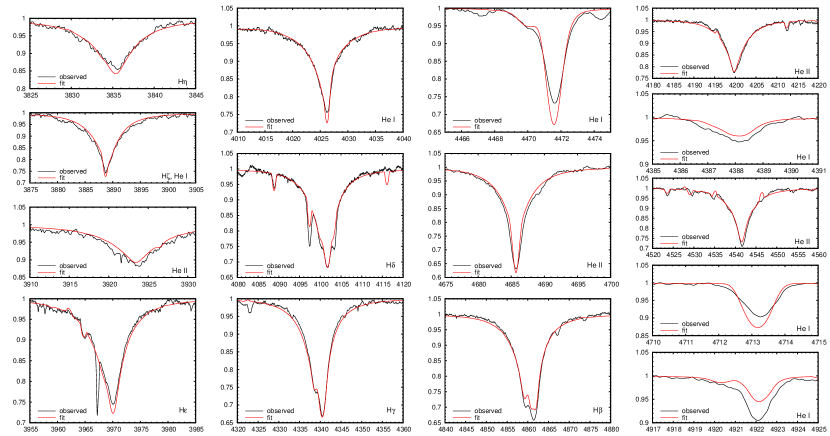
Figure 1: Comparison of the best-fit synthetic spectra (red line) and UVES spectra (black line) of HD~49798 in the visual region. Here we plot the normalised spectrum as a function of wavelength in Å.

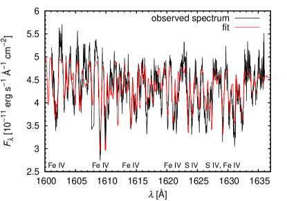
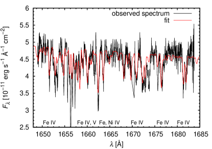
Figure 2: Comparison of the best-fit synthetic spectra (red line) and HST/GHRS spectra (black line) of HD~49798 in the UV region.

We used UVES and HST/GHRS spectra for the determination of the stellar parameters of HD~49798. All stellar parameters (see Table 2) were derived from UVES spectra except for abundances of Al, Fe, and Ni, for which we used HST/GHRS spectra. The model atmosphere grid for the stellar parameter determination, $T_{\mathrm{eff}}\in[44,\,46,\,48]\,\text{kK}$, $\log(g/1\,\text{cm}\,\text{s}^{-2})\in[4.15,\,4.40,\,4.65,\,4.90]$, and $\varepsilon_{\text{He}}\in[0.4,\,0.6,\,0.8]$, comprises the parameters derived by Kudritzki & Simon (1978) $T_{\mathrm{eff}}=47\,500\pm 2000\,\text{K}$, $\log(g/1\,\text{cm}\,\text{s}^{-2})=4.25\pm 0.2$, and $\varepsilon_{\text{He}}=0.5\pm 0.1$. After the determination of the helium abundance and the values of $T_{\mathrm{eff}}$  and $\log g$ from this grid, we determined the abundances of other elements using a model with fixed $\varepsilon_{\text{He}}$, $T_{\mathrm{eff}}$, and $\log g$. We iterated the process until convergence.

We adopted a slightly lower value of projected rotational velocity than Kudritzki & Simon (1978) $v\sin i=40\,\text{km}\,\text{s}^{-1}$ that provides a better fit of metallic lines. Figures 1 and 2 compare the observed UVES and HST/GHRS spectra with the best-fit synthetic spectra. The strongest lines used for the abundance determination are summarised in Table 3. We have not listed the UV lines of Fe and Ni, which are too numerous. The derived atmosphere parameters given in Table 2 agree with the results of Kudritzki & Simon (1978) within errors except the derived surface gravity, which is slightly higher. The nitrogen abundance is rather uncertain, because different nitrogen lines give very different abundances. The derived chemical composition deviates significantly from the solar composition (see Table 2). While carbon and oxygen are depleted, the abundances of nitrogen, iron, and nickel are a factor of a few higher than the solar value (Asplund et al., 2009).

The distance of HD~49798 was derived using GAIA DR2 data (Gaia Collaboration et al., 2016, 2018). With $V=8.287\pm 0.003\,$mag (Landolt & Uomoto, 2007) this gives the absolute magnitude $M_{V}=-0.24\pm 0.07\,$mag and with the bolometric correction $\text{BC}=27.58-6.80\log T_{\text{eff}}$ (Martins et al., 2005) the estimated luminosity is $L=4400\pm 400\,L_{\odot}$ (Martins et al., 2005, Eq. (5)). From this latter value, we derive a stellar radius of $R=1.05\,R_{\odot}\pm 0.06\,R_{\odot}$. With spectroscopic surface gravity, this gives the mass $M=1.46\pm 0.32\,M_{\odot}$, which nicely agrees with the mass of $1.50\pm 0.05\,M_{\odot}$ derived from the orbital solution (Mereghetti et al., 2009). With $i=85^{\circ}$ and the radius, and $v_{\text{rot}}\sin i$ from Table 2, we derive a rotational period of $1.3\pm 0.2\,$d. This is very close to the orbital period 1.55 d pointing to synchronised rotation.

The derived radius is lower than that estimated by Kudritzki & Simon (1978) due to lower adopted distance and higher derived gravity. As a result, predicted luminosity is also lower, which moves the position of the star closer to the canonical relationship between the stellar luminosity and X-ray luminosity (see Fig. 3, which is plotted assuming intrinsic wind X-ray luminosity of HD~49798 $3\times 10^{30}\,\text{erg}\,\text{s}^{-1}$, Mereghetti et al. 2013). Consequently, in this case the offset of the position of the star from the mean relationship was due to imprecise stellar parameters.

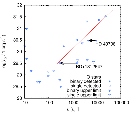
Figure 3: Relation between observed X-ray luminosity and the stellar luminosity for subdwarfs (adopted from Krtička et al. 2016). Blue symbols refer to individual subdwarfs: circles denote X-ray-detected subdwarfs, while triangles denote available upper X-ray detection limits, filled symbols denote subdwarfs in binaries, and empty symbols correspond to single objects. Overplotted is the extrapolation of the observed mean relation for O stars (Nazé, 2009, solid red line). The shift of the stellar parameters with respect to previous determinations is denoted using the black arrow.

5.2 Wind model

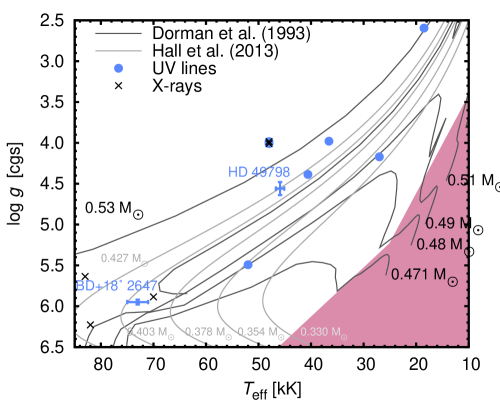
Figure 4: Position of studied stars in the $T_{\text{eff}}$ versus $\log g$ diagram. Red region denotes the parameter area with no predicted wind (Krtička et al., 2016). Overplotted are the evolutionary tracks of Dorman et al. (1993), post-RGB tracks of Hall et al. (2013) and the positions of subdwarfs with known mass-loss rates derived from observed UV wind-line profiles (blue circles) and subdwarfs with X-ray emission (black crosses). Adapted from Krtička et al. (2016).

We used our wind code to predict the structure of the stellar wind of HD~49798. The subdwarf lies well above the wind boundary in the $T_{\text{eff}}$ versus $\log g$ diagram (see Fig. 4), and consequently the predicted mass-loss rate is relatively large, $2.1\times 10^{-9}\,M_{\odot}\,\text{yr}^{-1}$ (see Table 2). Although iron and nickel are significantly overabundant with respect to the ratio of abundances of these elements relative to hydrogen, the predicted wind mass-loss rate is slightly lower than the value derived assuming solar chemical composition, $2.7\times 10^{-9}\,M_{\odot}\,\text{yr}^{-1}$. This is because (for solar chemical composition) the contribution of iron and nickel to the radiative force is surpassed by that of oxygen, which is depleted on the surface of HD~49798 by more than one order of magnitude with respect to the solar value. Moreover, the total mass fraction of heavier elements is close to the solar value. Similar results were derived for the influence of CNO cycle abundances on mass-loss rate for O stars (Krtička & Kubát, 2014).

The derived mass-loss rate is in close agreement with the value $2.8\times 10^{-9}\,M_{\odot}\,\text{yr}^{-1}$ derived from the fitting formula for subdwarfs (Krtička et al., 2016) assuming solar chemical composition. The mass-loss rates derived using the formula for ten times higher and ten times lower abundances of heavier elements are $8.8\times 10^{-9}\,M_{\odot}\,\text{yr}^{-1}$ and $8.7\times 10^{-10}\,M_{\odot}\,\text{yr}^{-1}$, respectively. The moderate difference between these values and the predicted mass-loss rate further demonstrates that the mass-loss rate is not particularly sensitive to abundances for HD~49798 parameters.

The X-ray luminosity of HD~49798 outside eclipses stems from the release of the gravitational potential energy during wind accretion on the compact companion. Within the classical Bondi-Hoyle-Lyttleton theory (Hoyle & Lyttleton, 1941; Bondi & Hoyle, 1944) the accretion luminosity is

$$L_{\text{X}}=\eta\frac{G^{3}M_{\text{X}}^{3}}{R_{\text{X}}D^{2}v^{4}}\dot{M},$$ (1)

where $M_{\text{X}}$ and $R_{\text{X}}$ are the mass and radius of the compact companion, $D$ is binary separation, $v$ is relative velocity, and $\eta$ is efficiency. If the wind velocity is much larger than the orbital velocity and is not affected by X-ray ionisation (Krtička et al., 2018; Sander et al., 2018), the wind terminal velocity can be inserted instead of the relative velocity $v=v_{\infty}$. Using wind parameters derived here (Table 2) in conjunction with $M_{\text{X}}=1.28\,M_{\odot}$ and $D=7.85\,R_{\odot}$ (Mereghetti et al., 2009), with $\eta=1$ we derive $L_{\text{X}}=1.2\times 10^{31}\,\text{erg}\,\text{s}^{-1}$ for typical parameters of a white dwarf and $L_{\text{X}}=4\times 10^{33}\,\text{erg}\,\text{s}^{-1}$ for a neutron star. The observed X-ray luminosity, with the updated distance provided by GAIA, is $\sim 10^{32}\,\text{erg}\,\text{s}^{-1}$ (Mereghetti et al., 2016). Consequently, to explain this luminosity in the case of a white dwarf, a decrease of the wind velocity due to X-ray ionisation is required. Instead, in the case of a neutron star, the predicted luminosity is higher than the observed one, requiring a low efficiency.

5.3 The X-ray eclipse light curve

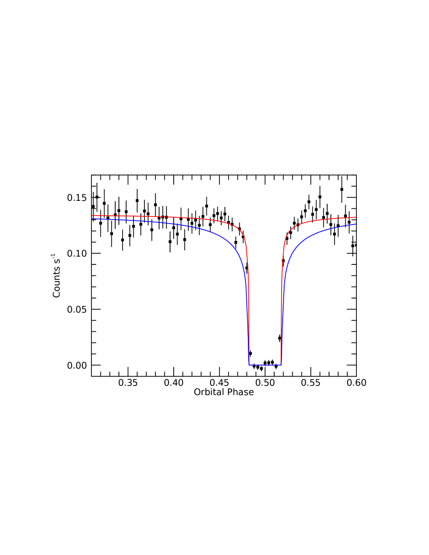
Figure 5: X-ray light curve of HD~49798 plotted during the eclipse. The red line shows the simulated eclipse light curve predicted assuming derived wind and stellar parameters. For a comparison, we also plot the light curve calculated assuming solar chemical composition (blue line).

X-ray observations with the XMM-Newton satellite showed that the eclipse ingress and egress are not sharp, suggesting that the X-rays emitted by the compact object are gradually absorbed in the wind of the sdO star. Using the wind model and surface composition derived in this work, we computed the absorption coefficient at different X-ray energies $\chi_{\nu}(r)$ and derived the expected profile for the resulting light curve around the time of the eclipse as an integral

$$F(\varphi)=F_{0}\,e^{-\tau(\varphi)},\qquad\tau(\varphi)=\int_{z_{\text{c}}(\varphi)}^{\infty}\chi_{\nu}(r(z))\,\text{d}z.$$ (2)

Here, $F_{0}$ is the X-ray flux from the companion and the integral is calculated numerically along the phase $\varphi$-dependent ray between the companion (located at $z=z_{\text{c}}$) and observer. We assumed a circular orbit with an inclination of $85^{\circ}$ that fits the length of the eclipse.

The calculation is compared to the observations in Fig. 5. The data were obtained from nine XMM-Newton observations covering the orbital phase of the eclipse (2008 May 10; 2011 May 02; August 18, 20, 25; September 3, 8; 2013 November 9; 2018 November 8). The figure shows the net light curve in the 0.15-0.5 keV energy range as measured with the EPIC pn instrument (the emission from HD~49798, as derived in the 4300 s of complete eclipse, has been subtracted). The red line shows the expected profile of the eclipse as computed with the wind abundances of HD 49798 derived in Sect. 5.2. For comparison, the blue line shows the profile that would be caused by a stellar wind with solar abundances. Although the statistical quality of the current X-ray data does not allow us to directly estimate the wind parameters, it is clear that the model derived with the proper abundances provides a good description of the X-ray data.

Table 4: Surface abundances of HD~49798 expressed relative to the total number density of baryons.

	HD~49798	Sun
$\log\tilde{\varepsilon}_{\text{CNO}}$	$-3.7\pm 0.2$	$-3.21$
$\log\tilde{\varepsilon}_{\text{Mg}}$	$-4.8\pm 0.5$	$-4.53$
$\log\tilde{\varepsilon}_{\text{Al}}$	$-5.5\pm 0.5$	$-5.68$
$\log\tilde{\varepsilon}_{\text{Si}}$	$-4.7\pm 0.2$	$-4.62$
$\log\tilde{\varepsilon}_{\text{Fe}}$	$-4.5\pm 0.2$	$-4.63$
$\log\tilde{\varepsilon}_{\text{Ni}}$	$-5.6\pm 0.2$	$-5.91$

5.4 Evolutionary implications

Bisscheroux et al. (1997) propose that the progenitor of HD~49798 was a star with an initial mass of $4-6\,M_{\odot}$ which during the asymptotic giant branch phase lost its envelope due to the common envelope event. This would imply that the star is in the phase of shell-helium burning with a degenerate C-O core. However, stars with C-O core mass implied by this scenario would instead ignite carbon (Siess, 2007, 2010). Moreover, massive post-AGB objects evolve on an extremely fast evolutionary timescale of the order of years (Vassiliadis & Wood, 1994; Miller Bertolami, 2016) and are therefore unlikely to be spotted in this stage. Alternatively, massive subdwarfs could be formed by the merger of white dwarfs, but this would likely lead to hydrogen deficient objects (Saio & Jeffery, 2002).

Popov et al. (2018) suggested that the subdwarf originates from an object with a helium-burning core. The companion could be either a white dwarf or a neutron star, but the white dwarf is preferred on the basis of known properties of X-rays and on evolutionary grounds (Bisscheroux et al., 1997). Moreover, the detected spin-up of the compact companion (Mereghetti et al., 2016) could be naturally explained as the consequence of cooling and contraction of a white dwarf (Popov et al., 2018).

HD~49798 shows very unusual chemical composition (see Table 2). Chemical peculiarities in blue horizontal branch stars are typically attributed to radiative diffusion (Hui-Bon-Hoa et al., 2000; Michaud et al., 2008; LeBlanc et al., 2009). A mass-loss rate of the order of $10^{-13}\,M_{\odot}\,\text{yr}^{-1}$ is required to explain the observed abundance anomalies in sdB stars (Unglaub & Bues, 2001). Higher mass-loss rates would not allow for the abundance separation in the atmosphere, while weaker wind would lead to a complete absence of helium (Unglaub & Bues, 2001; Michaud et al., 2015). Given the relatively high mass-loss rate found in HD~49798, the detected abundance anomalies are likely of evolutionary origin.

The high abundance of helium likely results from the stripping of the stellar envelope which led to the exposition of the stellar core, whose chemical composition was affected by hydrogen burning. A typical abundance ratio resulting from hydrogen burning by CNO cycles is $\log(\varepsilon_{\text{O}}/\varepsilon_{\text{N}})\approx-1$ (Maeder, 2009), while our analysis gives $\log(\varepsilon_{\text{O}}/\varepsilon_{\text{N}})=-1.5\pm 0.3$. The CNO equilibrium carbon-to-nitrogen ratio is $\log(\varepsilon_{\text{C}}/\varepsilon_{\text{N}})\approx-1.6$, which is consistent with our result $\log(\varepsilon_{\text{C}}/\varepsilon_{\text{N}})<-1.1$. To account for the enhanced abundance of helium, we scaled the derived elemental abundances relative to the baryonic number density $\tilde{\varepsilon}_{\text{el}}=\varepsilon_{\text{el}}/(\varepsilon_{\text{H}}+4\varepsilon_{\text{He}})$. From Table 4 it follows that the scaled abundances of most elements are consistent with solar chemical composition.

According to the evolutionary models, the helium-shell-burning subdwarf will fill its Roche lobe in approximately 40 000 – 65 000 yr (Brooks et al., 2017; Wang et al., 2017). On this evolutionary time-scale, the current mass loss as predicted here will not significantly contribute to mass transfer. The subdwarf lifetime is of the order of 1 Myr if the subdwarf is indeed burning its core helium (Paczyński, 1971), implying a larger contribution of the wind to the mass transfer. Mereghetti et al. (2009) showed that the further evolution of the system could lead to a second phase of mass transfer, which could ignite a SN Ia explosion. An alternative outcome of the evolution could be a double degenerate binary consisting of a neutron star (originating from the collapse of the compact companion) and a white dwarf (Brooks et al., 2017; Wang et al., 2017).

6 BD+18^∘ 2647

Subdwarf BD+18$^∘$ 2647 (Feige 67, PG 1239+178, $\alpha={12\,\text{h}\,41\;\text{m}\;51.79\,\text{s},}\;\delta={+17^{\circ}\,31^{\prime}\,19.75^{\prime\prime}}$, J2000) is a helium-poor star, which does not show any signs of a secondary companion (Latour et al., 2018). The subdwarf does not show any detectable X-ray emission with the upper limit of X-ray luminosity $3.2\times 10^{29}\,\text{erg}\,\text{s}^{-1}$ (La Palombara et al., 2014).

6.1 Determination of stellar parameters

Table 5: Wavelengths of the strongest lines (in Å) used for abundance determination in BD+18$^∘$ 2647.

C iii	977
C iv	1169, 1548, 1551
N iv	(923), (924), (955), 1719
N v	1239, 1243
O iv	923
F iv	1060
Ne v	1721
Si iv	1067, 1122, 1128, 1394, 1403
S v	1040, 1502, 1572
S vi	933, 944, 1001, 1118
Fe v	1068, 1200–1208, 1234–1799
Fe vi	986, 1009, 1042, 1200–1210, 1228–1766
Ni v	1001, 1200–1211, 1225–1620
Ni vi	954, 971, 980, 982, 1000, 1003, 1009, 1042, 1061,
	1065, 1068, 1070, 1071, 1075, 1076, 1200–1211,
	1227–1620

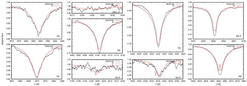
Figure 6: Comparison of synthetic spectra calculated for the derived parameters and UVES spectra of BD+18$^∘$ 2647 in the visual region.

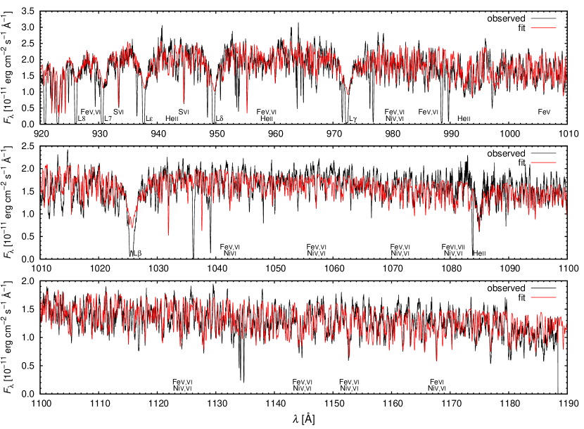
Figure 7: Comparison of synthetic spectra calculated for the derived parameters and FUSE spectra of BD+18$^∘$ 2647 in the UV region.

We used UVES, IUE, and FUSE spectra for the determination of the stellar parameters of BD+18$^∘$ 2647. The $T_{\text{eff}}$, $\log g$, and helium abundance were determined from the fit of optical and Lyman lines. The cores of predicted optical lines show emission and the cores of Lyman lines are affected by interstellar absorption. Therefore we fitted only the wings in the case of hydrogen Lyman lines and Balmer lines with central emission. The wings originate in the lower parts of the photosphere and are not severely affected by NLTE effects. For the determination of BD+18$^∘$ 2647 parameters, we first used a grid of NLTE models with a combination of $T_{\mathrm{eff}}\in[55,\,60,\,65,\,70,\,75,\,80,\,85,\,90]\,$kK, $\log(g/1\,\text{cm}\,\text{s}^{-2})\in[4.5,\,5.0,\,5.5,\,6.0]$, and $\varepsilon_{\text{He}}\in[0.01,\,0.032,\,0.1]$. During the final steps of parameter determination, we restricted the grid to $T_{\mathrm{eff}}\in[65,\,70,\,75]\,\text{kK}$, $\log(g/1\,\text{cm}\,\text{s}^{-2})\in[5.5,\,6.0,\,6.5]$, and $\varepsilon_{\text{He}}\in[0.01,\,0.032,\,0.1]$. Using these grids we obtained the values of $T_{\mathrm{eff}}$, $\log g$, and $\varepsilon_{\text{He}}$ listed in Table 2. The abundances of heavy elements were determined from the fit of UV spectra with a model calculated for derived values of stellar parameters. These steps were repeated until convergence was achieved.

The strongest lines used for abundance determination are given in Table 5. The comparison of the observed UVES and FUSE spectra and the best-fit synthetic spectra is given in Figs. 6 and 7. The derived atmosphere parameters and abundances given in Table 2 agree with the results of Latour et al. (2018) within errors, except for the derived effective temperature which is higher by about 12 kK. Latour et al. (2018) used optical spectra with lower resolution, consequently the problems with line centre emission could be one of the reasons for the difference in the derived temperatures. We were able to obtain a reasonable fit of hydrogen lines for lower $T_{\text{eff}}$, but this led to overly strong He i lines. Our derived effective temperature is lower than $T_{\text{eff}}=75\,000\,\text{K}$ derived by Bauer & Husfeld (1995).

To test the origin of the difference between the effective temperature derived by Latour et al. (2018) and our results, we smoothed the observed spectra by a Gaussian filter with $1.3\,\AA$ width that should roughly correspond to the spectra used in their analysis. We fitted full line profiles and the derived effective temperature was lower by about $6\,$kK. This shows that the adopted spectral resolution in combination with a different way of fitting could be one of the causes of the difference between the results. A higher abundance of iron, as derived by Latour et al. (2018), could be another reason for the difference. For some stars, the use of UV and optical observations may lead to discrepant results (Dixon et al., 2017), however in our case the UV spectra helped us mainly to constrain the grid of possible stellar parameters.

Because the derived effective temperature is higher than that derived by Latour et al. (2018), we further compared the predicted flux distribution with that derived using the VOSA tool (Bayo et al., 2008). The observed flux distribution in Fig. 8 is in close agreement with predictions with $E(B-V)=0.04\pm 0.02$ and assuming the Fitzpatrick & Massa (2007) extinction law. The derived reddening agrees with $E(B-V)=0.02\pm 0.02$ (Green et al., 2018), which corresponds to BD+18$^∘$ 2647 coordinates.

The distance was derived using GAIA DR2 data (Gaia Collaboration et al., 2016, 2018). With $V=11.63\pm 0.12\,$mag (Høg et al., 2000) this gives the absolute magnitude $M_{V}=4.07\pm 0.15\,$mag (with $E(B-V)=0.04\pm 0.02$) and with the bolometric correction $\text{BC}=27.58-6.80\log T_{\text{eff}}$ (Martins et al., 2005) the estimated luminosity is $L=290\pm 50\,L_{\odot}$ (Martins et al., 2005, Eq. (5)). From this, the stellar radius is $R=0.107\pm 0.011\,R_{\odot}$. With spectroscopic surface gravity this gives a mass of $M=0.38\pm 0.08\,M_{\odot}$.

The adopted bolometric correction fit (Martins et al., 2005) was derived for O stars with significantly lower effective temperature ($T_{\text{eff}}<45\,$kK) than derived here. To estimate the error connected with extrapolation of the bolometric correction, we calculated bolometric correction from our models using Eq. (1) of Lanz & Hubeny (2003) and the$V$ filter response curve from Mikulášek (private communication). The derived $BC=-5.60\pm 0.08\,$mag is only slightly lower than estimated from the fit of Martins et al. (2005), and therefore the resulting stellar parameters ($L=320\pm 50\,L_{\odot}$, $R=0.113\pm 0.011\,R_{\odot}$, and $M=0.41\pm 0.09\,M_{\odot}$) only differ within the derived uncertainties. We also note that the application of the frequently used bolometric corrections of Flower (1996, see also ,) to BD+18$^∘$ 2647 also leads to extrapolation, because these corrections were derived for stars with $T_{\text{eff}}<53\,$kK. Furthermore, Flower (1996) used high-order polynomial approximation, which may give erroneous results during extrapolation. In our case, the formula predicts bolometric correction which is 1 mag higher than adopted here leading to significantly lower mass.

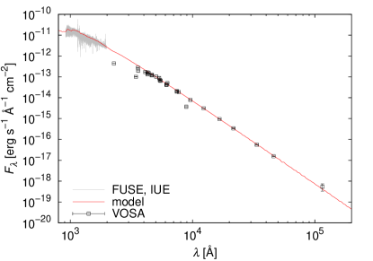
Figure 8: Comparison of predicted (red line) and observed flux distribution. The predicted flux was taken from the best-fit model and smoothed using a Gaussian filter. The observed flux distribution was taken from FUSE and IUE observations (grey lines) and from the optical and inferred photometry available in the VOSA database (squares with error bars).

The central parts of predicted hydrogen line profiles show emission that is missing in observed spectra (see Fig. 6). The missing emission in the observed spectra was already recognised by Latour et al. (2018), but the absence of emission is more striking in our analysis because we use spectra with higher resolution. To understand the origin of the emission in theoretical spectra, we calculated an additional NLTE model with fixed temperature derived assuming LTE. Even this model predicts emission in hydrogen line profiles. Therefore, the emission in predicted spectra is not caused by NLTE temperature inversion.

On the other hand, the structure of model atmosphere could be influenced by elements not included in our analysis. This could be connected with the possible appearance of weak lines in the optical spectrum which is not explained by the predicted spectrum. To test this, we calculated additional model atmospheres with ten times higher abundance of selected elements whose abundances were not determined from spectroscopy (Mg, Al, P, and Cr). However, we did not find any significant influence of these elements on hydrogen line profiles. Moreover, classical chemically peculiar stars show vertical abundance stratification (Stift & Alecian, 2012; Nesvacil et al., 2013), which may be present also in subdwarf atmospheres and affect the observed spectra (as suggested, e.g. by Geier 2013).

6.2 Wind model

Also, BD+18$^∘$ 2647 is located outside the wind limit in $T_{\text{eff}}$ versus $\log g$ diagram (Fig. 4, see also Krtička et al. 2016), however the mass-loss rate $7.2\times 10^{-11}\,M_{\odot}\,\text{yr}^{-1}$ predicted using Eq. (1) of Krtička et al. (2016) for BD+18$^∘$ 2647 parameters (Table 2) and solar chemical composition is two orders of magnitude lower than that of HD 49798. This value agrees reasonably well with the mass-loss rate of $3.9\times 10^{-11}\,M_{\odot}\,\text{yr}^{-1}$ derived from global models and solar chemical composition.

Due to its low mass-loss rate, the solar abundance wind of BD+18$^∘$ 2647 is mostly driven by lighter elements O, Ne, and Mg, while the contribution of iron is relatively small because numerous iron lines remain optically thin at low density (e.g. Puls et al., 2000; Vink & Cassisi, 2002; Krtička et al., 2016). Because these lighter elements are depleted on the surface of BD+18$^∘$ 2647  (see Table 2), it can be expected that the mass-loss rate calculated for realistic BD+18$^∘$ 2647 abundances is significantly lower than the mass-loss rate derived using solar abundances.

To test the presence of the wind for BD+18$^∘$ 2647 abundances we compared the magnitude of the radiative acceleration due to lines and scattering on free electrons $g^{\text{rad}}$ with the magnitude of the gravitational acceleration $g$. The winds are only possible if

$$g^{\text{rad}}>g.$$ (3)

The wind condition of Eq. (3) was tested using artificial wind models with fixed density and velocity structure and with mass-loss rate as a parameter. We assumed a linear velocity profile and the density profile was derived from the assumed mass-loss rate using the continuity equation. The application of Eq. (3) to these artificial models led to an upper limit of the mass-loss rate of BD+18$^∘$ 2647  of $10^{-12}\,M_{\odot}\,\text{yr}^{-1}$, while the wind condition is fulfilled for a mass-loss rate of $10^{-13}\,M_{\odot}\,\text{yr}^{-1}$.

Nevertheless, Eq. (3) gives a simply necessary but not sufficient condition for the presence of wind, because it does not compare the radiative and gravitational acceleration for a consistent wind solution. This likely explains why our global models failed to provide consistent wind models, although Eq. (3) would allow for a wind, albeit with a low mass-loss rate. To better understand this issue, we calculated additional simplified (but consistent) wind models that use the model atmosphere flux as an input for the calculation of the radiative force. Our tests with these simplified models showed that they are unable to pass through the sonic point with consistently calculated radiative force. Close inspection of the results revealed that the models are able to provide a converged solution with a first estimate of the radiative force, but further iterations failed. This corresponds to the fact that the models fulfilled the necessary condition for the presence of a wind Eq. (3) (which uses just one calculation of the radiative force), but failed to provide a consistent model.

Therefore, it is likely that BD+18$^∘$ 2647 is located close to the wind limit for its abundances. The proximity of the wind limit implies that the wind mass-loss rate is sensitive to metallicity. This can be further demonstrated using the mass-loss rate formula of Krtička et al. (2016), which for the increase of abundance by a factor of ten from the solar values predicts an increase of the mass-loss rate also by a factor of ten. This is a stronger metallicity dependence than in HD 49798. We cannot completely rule out the presence of wind in BD+18$^∘$ 2647 because the abundances of some elements that can drive wind were not determined from the spectra and could be higher than the solar values assumed here. Moreover, stars close to the wind limit may still have very weak purely metallic wind (Babel, 1995). The missing (or very weak) wind explains the absence of X-rays in BD+18$^∘$ 2647 ($L_{\text{X}}<3.2\times 10^{29}\,\text{erg}\,\text{s}^{-1}$, La Palombara et al., 2014).

6.3 Evolutionary implications

Hot subdwarfs are typically expected to be the products of binary evolution (Han et al., 2002). However, understanding the evolutionary state of BD+18$^∘$ 2647 is complicated by the unknown nature of a potential secondary. There is no evidence of a secondary from radial velocities, spectral energy distributions (Williams et al., 2001; Latour et al., 2018, see also Fig. 8), or from optical variability (Pancino et al., 2012; Marinoni et al., 2016). This could possibly mean that either the secondary is on a wide orbit, or that it is missing. Another problem is that the mass determined here is relatively small compared to typical subdwarfs (Heber, 2016), although the derived uncertainties are large and in principle even allow for more typical subdwarf masses.

From the missing signature of a companion it follows that BD+18$^∘$ 2647 could be formed by stable Roche-lobe overflow near the tip of the red giant branch, which may form wide binaries with low-mass subdwarfs (Podsiadlowski et al., 2008; Vos et al., 2019). Alternatively, BD+18$^∘$ 2647 could have been produced by the merger of either two helium white dwarfs (Han et al., 2002) or a helium white dwarf and a main sequence star (Zhang et al., 2018). However, the merger scenario likely implies a He-rich composition, which is not the case for this star. BD+18$^∘$ 2647 parameters also nicely correspond to stars in a post-red-giant-branch evolutionary phase (Fig. 4, Hall et al., 2013, see Reindl et al. 2014, Fig. 13), which have a degenerate helium core formed as a result of common envelope evolution. However, a companion on a short-period orbit is expected in this case. On the other hand, the derived mass is still within uncertainties close to the canonical subdwarf mass, which would allow for evolutionary scenarios that are more typical for subdwarfs (Heber, 2016).

The derived peculiar composition (Table 2) likely originates from radiative diffusion and gravitational settling in the atmosphere of the star (Latour et al., 2018). The upper limit of the mass-loss rate for BD+18$^∘$ 2647  has just the right value to moderate abundance stratification (Unglaub & Bues, 1998, 2001), while stronger wind would inhibit the abundance stratification (Unglaub & Bues, 2001; Vick et al., 2011). Within diffusion models, low abundance of helium is a result of gravitational settling. Chayer et al. (1995) provided equilibrium abundances of white dwarfs accounting for radiatively supported diffusion and, in agreement with our results, found enhanced surface abundance of iron, while carbon, nitrogen, neon, silicon, and sulphur were depleted at $T_{\mathrm{eff}}=70\,\text{kK}$.

It is not clear how is it possible that the star acquired abundance anomalies that would not likely develop if the star appeared at its current position on the HR diagram with solar abundances. Likely, the star initially had solar chemical composition, was located below the wind limit at some previous stage of its evolution, and developed abundance anomalies by diffusion. The abundance anomalies then persisted until the star attained the current parameters, although the wind predicted assuming a solar composition would have wiped out any peculiarities (Unglaub & Bues, 2001). It is also not clear why helium is still present in the atmosphere, because with absence of a wind, helium should be missing (Unglaub & Bues, 2001). Perhaps, some other process (e.g. turbulence, Michaud et al. 2011b) is responsible for this.

Despite similar abundance anomalies, in contrast to classical chemically peculiar stars, the subdwarfs and horizontal branch stars do not show rotationally modulated light variability (Pancino et al., 2012; Marinoni et al., 2016; Paunzen et al., 2019). Light variability in classical chemically peculiar stars typically originates due to flux redistribution in surface abundance spots (e.g. Prvák et al., 2015), which are supposed to be connected with strong surface magnetic field. Hot subdwarfs likely do not possess any strong global magnetic fields (Landstreet et al., 2012), which might explain the lack of rotationally modulated light variability.

7 Conclusions

We studied the implications of realistic surface abundances for the hot subdwarf wind mass-loss rates. We determined stellar parameters for two selected hydrogen-rich, hot subdwarfs from our own optical spectroscopy and from UV spectroscopy using TLUSTY NLTE atmosphere models. We predicted the wind mass-loss rates with our global wind model and compared the derived results with those predicted assuming solar chemical composition.

For HD 49798, we find an effective temperature in agreement with previous determinations and a mass that agrees with a binary solution. The chemical composition, with enhanced abundances of helium and nitrogen, appears to be a result of a previous process of hydrogen burning. The mass-loss rate predicted using realistic surface abundances does not significantly differ from that derived using solar abundances, because the mass fraction of heavier elements roughly corresponds to the solar chemical composition. The X-ray eclipse light curve can be nicely reproduced by absorption in the wind with the derived mass-loss rate and abundances, but not by a wind with solar abundances.

In the case of BD+18^∘ 2647 the derived stellar parameters agree reasonably with previous determinations with the exception of the effective temperature, which is about 12 kK higher than the recent determination, but is still in the range of values available in the literature. The discrepant temperature is probably due to an overly weak dependence of line profiles on the stellar parameters and the appearance of emission in the cores of predicted absorption lines. The subsolar abundance of light elements and the overabundance of iron can be interpreted as a result of radiative diffusion and gravitational settling. As a result of this, the homogeneous wind is missing for determined abundances, while the wind would exist at solar metallicity. On the other hand, a stronger wind would likely have effaced all peculiarities.

Although we used UV and optical spectra to determine the abundances, the lines of some elements that are important for driving wind are inaccessible in the available spectral regions. From our models it follows that about one-third of the line driving still comes from such elements. This contributes to the uncertainty related to mass-loss rate predictions.

We conclude that while the precise abundances are not very important for the strength of the wind in cases where the surface abundances are affected by hydrogen burning, abundances have a significant effect when diffusion processes come into play. Therefore, abundance variations and imprecise stellar parameters may be one of the reasons for the large scatter of hot subdwarf X-ray luminosity when plotted as a function of bolometric luminosity.