Reachability Analysis of Self Modifying Code

Abstract

A Self modifying code is code that modifies its own instructions during execution time. It is nowadays widely used, especially in malware to make the code hard to analyse and to detect by anti-viruses. Thus, the analysis of such self modifying programs is a big challenge. Pushdown systems (PDSs) is a natural model that is extensively used for the analysis of sequential programs because they allow to accurately model procedure calls and mimic the program’s stack. In this work, we propose to extend the PushDown System model with self-modifying rules. We call the new model Self-Modifying PushDown System (SM-PDS). A SM-PDS is a PDS that can modify its own set of transitions during execution. We show how SM-PDSs can be used to naturally represent self-modifying programs and provide efficient algorithms to compute the backward and forward reachable configurations of SM-PDSs. We implemented our techniques in a tool and obtained encouraging results. In particular, we successfully applied our tool for the detection of self-modifying malware.

I Introduction

Self-modifying code is code that modifies its own instructions during execution time. It is nowadays widely used, mainly to make programs hard to understand. For example, self-modifying code is extensively used to protect software intellectual property, since it makes reverse code engineering harder. It is also abundantly used by malware writers in order to obfuscate their malicious code and make it hard to analyse by static analysers and anti-viruses.

There are several kinds of implementations for self-modifying codes. Packing [CT08] consists in applying compression techniques to make the size of the executable file smaller. This converts the executable file to a form where the executable content is hidden. Then, the code is ”unpacked” at runtime before execution. Such packed code is self-modifying. Encryption is another technique to hide the code. It uses some kind of invertible operations to hide the executable code with an encryption key. Then, the code is ”decrypted” at runtime prior to execution. Encrypted programs are self-modifying. These two forms of self-modifying codes have been well studied in the litterature and could be handled by several unpacking tools such as [Tea, Kar].

In this work, we consider another kind of self-modifying code, caused by self-modifying instructions, where code is treated as data that can thus be read and written by self-modifying instructions. These self-modifying instructions are usually mov instructions, since mov can access memory, and read and write to it. For example, consider the program shown in Figure1. For simplification matters, we suppose that the addresses’ length is 1 byte. The binary code is given in the left side, while in the right side, we give its corresponding assembly code obtained by translating syntactically the binary code at each address. For example, ff is the binary code of the instruction push, thus, the first line is translated to push 0x3, the second line to push 0b, etc. Let us execute this code. First, we execute push 0x3, then push 0b, then mov 0x2 0xc. This last instruction will replace the first byte at address 0x2 by 0xc. Thus, at address 0x2, ff 0b is replaced by 0c 0b. Since 0c is the binary code of jmp, this means the instruction push 0b is replaced by jmp 0xb. Therefore, this code is self-modifying. If we treat it blindly, without looking at the semantics of the different instructions, we will extract from it the Control Flow Graph CFG a, whereas its correct Control Flow Graph is CFG b. You can see that the mov instruction was able to modify the instructions of the program successfully via its ability to read and write the memory.

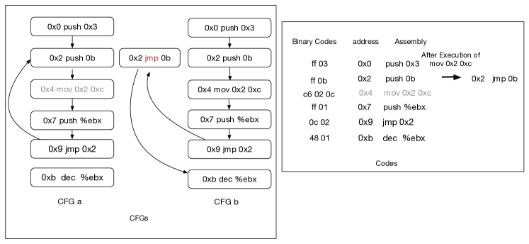
Figure 1: A Simple Example of Self-modifying Codes

In this paper, we consider the reachability analysis of self-modifying programs where the code is modified by mov instructions. To this aim, we first need to find an adequate model for such programs. PushDown Systems (PDS) are known to be a natural model for sequential programs [Sch02], as they allow to track the contexts of the different calls in the program. Moreover, PushDown Systems allow to record and mimic the program’s stack, which is very important for malware detection. Indeed, to check whether a program is malicious, anti-viruses start by identifying the calls it makes to the API functions. To evade these checks, malware writers try to obfuscate the calls they make to the Operating System by using pushes and jumps. Thus, it is important to be able to track the stack to detect such obfuscated calls. This is why PushDown Systems were used in [ST12, ST13] to model binary programs in order to perform malware detection. However, these works do not consider malwares that use self-modifying code, as PushDown Systems are not able to model self-modifying instructions.

To overcome this limitation, we propose in this work to extend the PushDown System model with self-modifying rules. We call the new model Self-Modifying PushDown System (SM-PDS). Roughly speaking, a SM-PDS is a PDS that can modify its own set of transitions during execution. We show how SM-PDSs can be used to naturally represent self-modifying programs. It turns out that SM-PDSs are equivalent to standard PDSs. We show how to translate a SM-PDS to a standard PDS. This translation is exponential. Thus, performing the reachability analysis on the equivalent PDS is not efficient. We propose then direct algorithms to compute the forward ($post^{*}$) and backward ($pre^{*}$) reachability sets for SM-PDSs. This allows to efficiently perform reachability analysis for self-modifying programs. Our algorithms are based on (1) representing regular (potentially infinite) sets of configurations of SM-PDSs using finite state automata, and (2) applying saturation procedures on the finite state automata in order to take into account the effect of applying the rules of the SM-PDS. We implemented our algorithms in a tool that takes as input either an SM-PDS or a self-modifying program. Our experiments show that our direct techniques are much more efficient than translating the SM-PDS to an equivalent PDS and then applying the standard reachability algorithms for PDSs [BEM97, EHRS00, Sch02]. Moreover, we successfully applied our tool to the analysis of several self-modifying malwares.

This paper is an expanded version of the conference paper [TY17]. Compared to [TY17], in this expanded version, we propose new algorithms for computing the forward and backward reachable configurations for SM-PDSs, and we provide the detailed proofs that show the correctness of our constructions.

Outline. The rest of the paper is structured as follows: Section 2 introduces our new model and shows how to translate a SM-PDS to an equivalent pushdown system. In Section 3, we give the translation from a binary code to a SM-PDS. In Section 4, we define finite automata to represent regular (potentially infinite) sets of configurations of SM-PDSs. Sections 5 and 6 give our algorithms to compute the backward and forward reachability sets of SM-PDSs. Section 7 describes our experiments.

Related Work.

Reachability analysis of pushdown systems was considered in [BEM97, EHRS00]. Our algorithms are extensions of the saturation approach of these works.

Model checking and static analysis approaches have been widely used to analyze binary programs, for instance, in [BDD⁺01, BRK⁺05, SL03, CJS⁺05, KKSV05, ST13, CJS⁺05]. These works cannot handle self-modifying code.

Cai et al. [CSV07] use a Hoare-logic-style framework to describe self-modifying code by applying local reasoning and separation logic, and treating program code uniformly as regular data structure. However, [CSV07] requires programs to be manually annotated with invariants. In [CT08], the authors describe a formal semantics for self-modifying codes, and use that semantics to represent self-unpacking code. This work only deals with packing and unpacking behaviours, it cannot capture self-modifying instructions as we do. In [BMRP09], Bonfante et al. provide an operational semantics for self-modifying programs and show that they can be constructively rewritten to a non-modifying program. All these specifications [BMRP09, CSV07, CT08] are too abstract to be used in practice.

In [AMDB06], the authors propose a new representation of self-modifying code named State Enhanced-Control Flow Graph (SE-CFG). SE-CFG extends standard control flow graphs with a new data structure, keeping track of the possible states programs can reach, and with edges that can be conditional on the state of the target memory location. It is not easy to analyse a binary program only using its SE-CFG, especially that this representation does not allow to take into account the stack of the program.

[BLP16] propose abstract interpretation techniques to compute an over-approximation of the set of reachable states of a self-modifying program, where for each control point of the program, an over-approximation of the memory state at this control point is provided. [RM10] combine static and dynamic analysis techniques to analyse self-modifying programs. Unlike our self-modifying pushdown systems, these techniques [BLP16, RM10] cannot handle the program’s stack.

Finally, unpacking binary code is considered in [CDKT09, KPY07, RHD⁺06, CT08]. These works do not consider self-modifying mov instructions.

II Self-modifying Pushdown Systems

II-A Definition

We introduce in this section our new model: Self-modifying Pushdown Systems.

Definition 1.

A Self-modifying Pushdown System (SM-PDS) is a tuple $\mathcal{P}=(P,\Gamma,\Delta,\Delta_{c})$, where $P$ is a finite set of control points, $\Gamma$ is a finite set of stack symbols, $\Delta\subseteq(P\times\Gamma)\times(P\times\Gamma^{*})$ is a finite set of transition rules, and $\Delta_{c}\subseteq P\times(\Delta\cup\Delta_{c})\times(\Delta\cup\Delta_{c})\times P$ is a finite set of modifying transition rules. If $((p,\gamma),(p^{\prime},w))\in\Delta$, we also write $\langle p,\gamma\rangle\hookrightarrow\langle p^{\prime},w\rangle\in\Delta$. If $(p,r_{1},r_{2},p^{\prime})\in\Delta_{c}$, we also write $p\stackrel{{\scriptstyle(r_{1},r_{2})}}{{\lhook\joinrel\relbar\joinrel\relbar\joinrel\relbar\joinrel\relbar\joinrel\rightarrow}}p^{\prime}\in\Delta_{c}$. A Pushdown System (PDS) is a SM-PDS where $\Delta_{c}=\emptyset$.

Intuitively, a Self-modifying Pushdown System is a Pushdown System that can dynamically modify its set of rules during the execution time: rules $\Delta$ are standard PDS transition rules, while rules $\Delta_{c}$ modify the current set of transition rules: $\langle p,\gamma\rangle\hookrightarrow\langle p^{\prime},w\rangle\in\Delta$ expresses that if the SM-PDS is in control point $p$ and has $\gamma$ on top of its stack, then it can move to control point $p^{\prime}$, pop $\gamma$ and push $w$ onto the stack, while $p\stackrel{{\scriptstyle(r_{1},r_{2})}}{{\lhook\joinrel\relbar\joinrel\relbar\joinrel\relbar\joinrel\relbar\joinrel\rightarrow}}p^{\prime}\in\Delta_{c}$ expresses that when the PDS is in control point $p$, then it can move to control point $p^{\prime}$, remove the rule $r_{1}$ from its current set of transition rules, and add the rule $r_{2}$. Formally, a configuration of a SM-PDS is a tuple $c=(\langle p,w\rangle,\theta)$ where $p\in P$ is the control point, $w\in\Gamma^{*}$ is the stack content, and $\theta\subseteq\Delta\cup\Delta_{c}$ is the current set of transition rules of the SM-PDS. $\theta$ is called the current phase of the SM-PDS. When the SM-PDS is a PDS, i.e., when $\Delta_{c}=\emptyset$, a configuration is a tuple $c=(\langle p,w\rangle,\Delta)$, since there is no changing rule, so there is only one possible phase. In this case, we can also write $c=\langle p,w\rangle$. Let $\mathcal{C}$ be the set of configurations of a SM-PDS. A SM-PDS defines a transition relation $\Rightarrow_{\mathcal{P}}$ between configurations as follows: Let $c=(\langle p,w\rangle,\theta)$ be a configuration, and let $r$ be a rule in $\theta$, then:

1. if $r\in\Delta_{c}$ is of the form $r=p\stackrel{{\scriptstyle(r_{1},r_{2})}}{{\lhook\joinrel\relbar\joinrel\relbar\joinrel\relbar\joinrel\relbar\joinrel\rightarrow}}p^{\prime}$, such that $r_{1}\in\theta$, then $(\langle p,w\rangle,\theta)\Rightarrow_{\mathcal{P}}(\langle p^{\prime},w\rangle,\theta^{\prime})$, where $\theta^{\prime}=(\theta\setminus\{r_{1}\})\cup\{r_{2}\}$. In other words, the transition rule $r$ updates the current set of transition rules $\theta$ by removing $r_{1}$ from it and adding $r_{2}$ to it.

2. if $r\in\Delta$ is of the form $r=\langle p,\gamma\rangle\hookrightarrow\langle p^{\prime},w^{\prime}\rangle\in\Delta$, then $(\langle p,\gamma w\rangle,\theta)\Rightarrow_{\mathcal{P}}(\langle p^{\prime},w^{\prime}w\rangle,\theta)$. In other words, the transition rule $r$ moves the control point from $p$ to $p^{\prime}$, pops $\gamma$ from the stack and pushes $w^{\prime}$ onto the stack. This transition keeps the current set of transition rules $\theta$ unchanged.

Let $\Rightarrow_{\mathcal{P}}^{*}$ be the transitive, reflexive closure of $\Rightarrow_{\mathcal{P}}$. We define $\stackrel{{\scriptstyle i}}{{\Rightarrow}}$ as follows: $c\stackrel{{\scriptstyle i}}{{\Rightarrow}}c^{\prime}$ iff there exists a sequence of configurations $c_{0}\Rightarrow_{\mathcal{P}}c_{1}\Rightarrow_{\mathcal{P}}...\Rightarrow_{\mathcal{P}}c_{i}$ s.t. $c_{0}=c$ and $c_{i}=c$ Given a configuration $c$, the set of immediate predecessors (resp. successors) of $c$ is $pre_{\mathcal{P}}(c)=\{c^{\prime}\in\mathcal{C}\;:\;c^{\prime}\Rightarrow_{\mathcal{P}}c\}$ (resp. $post_{\mathcal{P}}(c)=\{c^{\prime}\in\mathcal{C}\;:\;c\Rightarrow_{\mathcal{P}}c^{\prime}\}$). These notations can be generalized straightforwardly to sets of configurations. Let $pre_{\mathcal{P}}^{*}$ (resp. $post_{\mathcal{P}}^{*}$) denote the reflexive-transitive closure of $pre_{\mathcal{P}}$ (resp. $post_{\mathcal{P}}$). We omit the subscript $\mathcal{P}$ when it is understood from the context.

Example 1.

Let $\mathcal{P}=(P,\Gamma,\Delta,\Delta_{c})$ be a SM-PDS where $p=\{p_{1},p_{2},p_{3},p_{4}\}$, $\Gamma=\{\gamma_{1},\gamma_{2},\gamma_{3}\}$, $\Delta=\{r_{1}:\langle p_{1},\gamma_{1}\rangle\hookrightarrow\langle p_{2},\gamma_{2}\gamma_{1}\rangle,r_{2}:\langle p_{2},\gamma_{2}\rangle\hookrightarrow\langle p_{3},\epsilon\rangle,r_{3}:\langle p_{4},\gamma_{1}\rangle\hookrightarrow\langle p_{2},\gamma_{2}\gamma_{3}\rangle\}$, $\Delta_{c}=\{r^{\prime}:p_{3}\stackrel{{\scriptstyle(r_{1},r_{3})}}{{\lhook\joinrel\relbar\joinrel\relbar\joinrel\relbar\joinrel\relbar\joinrel\rightarrow}}p_{4}\}$. Let $c_{0}=(\langle p_{1},\gamma_{1}\gamma_{1}\rangle,\theta_{0})$ where $\theta_{0}=\{r_{1},r_{2},r^{\prime}\}$. Applying rule $r_{1}$, we get $(\langle p_{1},\gamma_{1}\gamma_{1}\rangle,\theta_{0})\Rightarrow_{\mathcal{P}}(\langle p_{2},\gamma_{2}\gamma_{1}\gamma_{1}\rangle,\theta_{0})$. Then, applying rule $r_{2}$, we get $(\langle p_{2},\gamma_{2}\gamma_{1}\gamma_{1}\rangle,\theta_{0})\Rightarrow_{\mathcal{P}}(\langle p_{3},\gamma_{1}\gamma_{1}\rangle,\theta_{0})$. Then, applying rule $r^{\prime}$, we get $(\langle p_{3},\gamma_{1}\gamma_{1}\rangle,\theta_{0})\Rightarrow_{\mathcal{P}}(\langle p_{4},\gamma_{1}\gamma_{1}\rangle,\theta_{1})$ where $r^{\prime}$ is self-modifying, thus, it leads the SM-PDS from phase $\theta_{0}=\{r_{1},r_{2},r^{\prime}\}$ to phase $\theta_{1}=\theta_{0}\setminus\{r_{1}\}\cup\{r_{3}\}=\{r_{2},r_{3},r^{\prime}\}$. Then, applying rule $r_{3}$, we get $(\langle p_{4},\gamma_{1}\gamma_{1}\rangle,\theta_{1})\Rightarrow_{\mathcal{P}}(\langle p_{2},\gamma_{2}\gamma_{3}\gamma_{1}\rangle,\theta_{1})$. Then, applying rule $r_{2}$ again, we get $(\langle p_{2},\gamma_{2}\gamma_{3}\gamma_{1}\rangle,\theta_{1})\Rightarrow_{\mathcal{P}}(\langle p_{3},\gamma_{3}\gamma_{1}\rangle,\theta_{1})$.

II-B From SM-PDSs to PDSs

A SM-PDS can be described by a PDS. This is due to the fact that the number of phases is finite, thus, we can encode phases in the control points of the PDS: Let $\mathcal{P}=(P,\Gamma,\Delta,\Delta_{c})$ be a SM-PDS, we compute the PDS $\mathcal{P}^{\prime}=(P^{\prime},\Gamma,\Delta^{\prime})$ as follows: $P^{\prime}=P\times 2^{\Delta\cup\Delta_{c}}$. Initially, $\Delta^{\prime}=\emptyset$. For every $\theta\in 2^{\Delta\cup\Delta_{c}}$, $r\in\theta$:

1. If $r=\langle p,\gamma\rangle\hookrightarrow(p^{\prime},w)\in\Delta$, we add $\langle(p,\theta),\gamma\rangle\hookrightarrow\langle(p^{\prime},\theta),w\rangle$ to $\Delta^{\prime}$

2. if $r=p\stackrel{{\scriptstyle(r_{1},r_{2})}}{{\lhook\joinrel\relbar\joinrel\relbar\joinrel\relbar\joinrel\relbar\joinrel\rightarrow}}p^{\prime}\in\Delta_{c}$, then for every $\gamma\in\Gamma$, we add $\langle(p,\theta),\gamma\rangle\hookrightarrow\langle(p^{\prime},\theta^{\prime}),\gamma\rangle$ to $\Delta^{\prime}$, where $\theta^{\prime}=(\theta\setminus\{r_{1}\})\cup\{r_{2}\}$.

It is easy to see that:

Proposition 1.

$(\langle p,w\rangle,\theta)\Rightarrow_{\mathcal{P}}(\langle p^{\prime},w^{\prime}\rangle,\theta^{\prime})$ iff $\langle(p,\theta),w\rangle\Rightarrow_{\mathcal{P}^{\prime}}\langle(p^{\prime},\theta^{\prime}),w^{\prime}\rangle$.

Proof: 

$\Rightarrow:$ We will show that if $(\langle p,w\rangle,\theta)\Rightarrow_{\mathcal{P}}(\langle p^{\prime},w^{\prime}\rangle,\theta^{\prime})$, then we have $\langle(p,\theta),w\rangle\Rightarrow_{\mathcal{P}^{\prime}}\langle(p^{\prime},\theta^{\prime}),w^{\prime}\rangle$. There are two cases depending on the form of the rule that led to this transition.

• Case $\theta=\theta^{\prime}:$ it means that the transition does not correspond to a self-modifying transition rule. Thus there is a rule $r\in\theta$ of the form $r=\langle p,\gamma\rangle\hookrightarrow\langle p^{\prime},u^{\prime}\rangle$ that led to this transition. Let $u$ be such that $w=\gamma u,w^{\prime}=u^{\prime}u$. By the construction rule of the PDS $\mathcal{P}^{\prime}$, we have $\langle(p,\theta),\gamma\rangle\hookrightarrow\langle(p^{\prime},\theta),u^{\prime}\rangle\in\Delta^{\prime}$. Therefore, $\langle(p,\theta),\gamma u\rangle\Rightarrow_{\mathcal{P}^{\prime}}\langle(p^{\prime},\theta),u^{\prime}u\rangle$ holds. This implies that $\langle(p,\theta),w\rangle\Rightarrow_{\mathcal{P}^{\prime}}\langle(p^{\prime},\theta),w^{\prime}\rangle$.

• Case $\theta\neq\theta^{\prime}:$ it means that the transition corresponds to a self-modifying transition rule. Thus there is a rule $r\in\theta$ of the form $p\stackrel{{\scriptstyle(r_{1},r_{2})}}{{\lhook\joinrel\relbar\joinrel\relbar\joinrel\relbar\joinrel\relbar\joinrel\rightarrow}}p^{\prime}$ that led to this transition. Let $u$ be such that $w=\gamma u,w^{\prime}=\gamma u$. By the construction rule of the PDS $\mathcal{P}^{\prime}$, we have $\langle(p,\theta),\gamma\rangle\hookrightarrow\langle(p^{\prime},\theta^{\prime}),\gamma\rangle\in\Delta^{\prime}$ where $\theta^{\prime}=(\theta\backslash\{r_{1}\})\cup\{r_{2}\}$. Therefore, $\langle(p,\theta),\gamma u\rangle\Rightarrow_{\mathcal{P}^{\prime}}\langle(p^{\prime},\theta^{\prime}),\gamma u\rangle$ holds. This implies that $\langle(p,\theta),w\rangle\Rightarrow_{\mathcal{P}^{\prime}}\langle(p^{\prime},\theta^{\prime}),w^{\prime}\rangle$.

$\Leftarrow:$ We will show that if $\langle(p,\theta),w\rangle\Rightarrow_{\mathcal{P}^{\prime}}\langle(p^{\prime},\theta^{\prime}),w^{\prime}\rangle$, then $(\langle p,w\rangle,\theta)\Rightarrow_{\mathcal{P}}(\langle p^{\prime},w^{\prime}\rangle,\theta^{\prime})$. Let $\gamma\in\Gamma,u,u^{\prime}\in\Gamma^{*}$ be such that $w=\gamma u,w^{\prime}=u^{\prime}u.$ There are two cases.

• Case $\theta=\theta^{\prime}.$ Let $r=\langle(p,\theta),\gamma\rangle\hookrightarrow\langle(p^{\prime},\theta),u^{\prime}\rangle\in\Delta^{\prime}$ be the rule that led to the transition. By the construction of PDS $\mathcal{P^{\prime}}$, there must exist a rule $r\in\theta$ such that $r=\langle p,\gamma\rangle\hookrightarrow\langle p^{\prime},u^{\prime}\rangle$. Therefore, $(\langle p,\gamma u\rangle,\theta)\Rightarrow_{\mathcal{P}}(\langle p,u^{\prime}u\rangle,\theta)$ holds. This implies that $(\langle p,w\rangle,\theta)\Rightarrow_{\mathcal{P}}(\langle p,w^{\prime}\rangle,\theta^{\prime})$.

• Case $\theta\neq\theta^{\prime}.$ Let $r=\langle(p,\theta),\gamma\rangle\hookrightarrow\langle(p^{\prime},\theta^{\prime}),\gamma\rangle\in\Delta^{\prime}$ be the rule leading to the transition and $u^{\prime}=\gamma.$ By the construction of PDS $\mathcal{P^{\prime}}$, there must exist a rule $r\in\theta$ such that $r=p\stackrel{{\scriptstyle(r_{1},r_{2})}}{{\lhook\joinrel\relbar\joinrel\relbar\joinrel\relbar\joinrel\relbar\joinrel\rightarrow}}p^{\prime}$ where $\theta^{\prime}=(\theta\backslash\{r_{1}\})\cup\{r_{2}\}$. Therefore, $(\langle p,\gamma u\rangle,\theta)\Rightarrow_{\mathcal{P}}(\langle p^{\prime},\gamma u\rangle,\theta^{\prime})$ holds. This implies that $(\langle p,w\rangle,\theta)\Rightarrow_{\mathcal{P}}(\langle p,w^{\prime}\rangle,\theta^{\prime})$.

$\;\;\Box$

Thus, we get:

Theorem 1.

Let $\mathcal{P}=(P,\Gamma,\Delta,\Delta_{c})$ be a SM-PDS, we can compute an equivalent PDS $\mathcal{P}^{\prime}=(P^{\prime},\Gamma,\Delta^{\prime})$ such that $|\Delta^{\prime}|=\big{(}|\Delta|+|\Delta_{c}|\cdot|\Gamma|\big{)}\cdot 2^{\mathcal{O}(|\Delta|+|\Delta_{c}|)}$ and $|P^{\prime}|=|P|\cdot 2^{\mathcal{O}(|\Delta|+|\Delta_{c}|)}$.

II-C From SM-PDSs to Symbolic PDSs

Instead of recording the phases $\theta$ of the SM-PDS in the control points of the equivalent PDS, we can have a more compact translation from SM-PDSs to symbolic PDSs [Sch02], where each SM-PDS rule is represented by a single, symbolic transition, where the different values of the phases are encoded in a symbolic way using relations between phases:

Definition 2.

A symbolic pushdown system is a tuple $\mathcal{P}=(P,\Gamma,\delta)$, where $P$ is a set of control points, $\Gamma$ is the stack alphabet, and $\delta$ is a set of symbolic rules of the form: $\langle p,\gamma\rangle\stackrel{{\scriptstyle R}}{{\lhook\joinrel\relbar\joinrel\relbar\joinrel\relbar\joinrel\relbar\joinrel\rightarrow}}\langle p^{\prime},w\rangle$, where $R\subseteq 2^{\Delta\cup\Delta_{c}}\times 2^{\Delta\cup\Delta_{c}}$ is a relation.

A symbolic PDS defines a transition relation $\leadsto_{\mathcal{P}}$ between SM-PDS configurations as follows: Let $c=(\langle p,\gamma w^{\prime}\rangle,\theta)$ be a configuration and let $\langle p,\gamma\rangle\stackrel{{\scriptstyle R}}{{\lhook\joinrel\relbar\joinrel\relbar\joinrel\relbar\joinrel\relbar\joinrel\rightarrow}}\langle p^{\prime},w\rangle$ be a rule in $\delta$, then: $(\langle p,\gamma w^{\prime}\rangle,\theta)\leadsto_{\mathcal{P}}(\langle p^{\prime},ww^{\prime}\rangle,\theta^{\prime})$ for $(\theta,\theta^{\prime})\in R$. Let $\leadsto_{\mathcal{P}}^{*}$ be the transitive, reflexive closure of $\leadsto_{\mathcal{P}}$. Then, given a SM-PDS $\mathcal{P}=(P,\Gamma,\Delta,\Delta_{c})$, we can compute an equivalent symbolic PDS $\mathcal{P}^{\prime}=(P,\Gamma,\Delta^{\prime})$ such that: Initially, $\Delta^{\prime}=\emptyset$;

• For every $\langle p,\gamma\rangle\hookrightarrow\langle p^{\prime},w\rangle\in\Delta$, add $\langle p,\gamma\rangle\stackrel{{\scriptstyle R_{id}}}{{\lhook\joinrel\relbar\joinrel\relbar\joinrel\relbar\joinrel\relbar\joinrel\rightarrow}}\langle p^{\prime},w\rangle$ to $\Delta^{\prime}$, where $R_{id}$ is the identity relation.

• For every $r=p\stackrel{{\scriptstyle(r_{1},r_{2})}}{{\lhook\joinrel\relbar\joinrel\relbar\joinrel\relbar\joinrel\relbar\joinrel\rightarrow}}p^{\prime}\in\Delta_{c}$ and every $\gamma\in\Gamma$, add $\langle p,\gamma\rangle\stackrel{{\scriptstyle R}}{{\lhook\joinrel\relbar\joinrel\relbar\joinrel\relbar\joinrel\relbar\joinrel\rightarrow}}\langle p^{\prime},\gamma\rangle$ to $\Delta^{\prime}$, where $R=\{(\theta_{1},\theta_{2})\in 2^{\Delta\cup\Delta_{c}}\times 2^{\Delta\cup\Delta_{c}}\mid r\in\theta_{1}\text{ and }\theta_{2}=(\theta_{1}\setminus\{r_{1}\})\cup\{r_{2}\}\}$.

It is easy to see that:

Proposition 2.

$(\langle p,w\rangle,\theta)\Rightarrow_{\mathcal{P}}(\langle p^{\prime},w^{\prime}\rangle,\theta^{\prime})$ iff $(\langle p,w\rangle,\theta)\leadsto_{\mathcal{P^{\prime}}}(\langle p^{\prime},w^{\prime}\rangle,\theta^{\prime})$.

Proof: 

$\Rightarrow:$ we will show that if $(\langle p,w\rangle,\theta)\Rightarrow_{\mathcal{P}}(\langle p^{\prime},w^{\prime}\rangle,\theta^{\prime})$, then $(\langle p,w\rangle,\theta)\leadsto_{\mathcal{P^{\prime}}}(\langle p^{\prime},w^{\prime}\rangle,\theta^{\prime})$. There are two cases depending on the form of the rule that led to this transition.

• Case $\theta=\theta^{\prime}$, it means that the transition does not correspond to a self-modifying transition rule. Thus there is a rule $r\in\theta$ of the form $r=\langle p,\gamma\rangle\hookrightarrow\langle p^{\prime},u^{\prime}\rangle$ that led to this transition. Let $u$ be such that $w=\gamma u,w^{\prime}=u^{\prime}u$. By construction of the symbolic pushdown system $\mathcal{P^{\prime}}$, $\langle p,\gamma\rangle\stackrel{{\scriptstyle R_{id}}}{{\lhook\joinrel\relbar\joinrel\relbar\joinrel\relbar\joinrel\relbar\joinrel\rightarrow}}\langle p^{\prime},u^{\prime}\rangle\in\Delta^{\prime}$, therefore, $(\langle p,\gamma u\rangle,\theta)\leadsto_{\mathcal{P^{\prime}}}(\langle p^{\prime},u^{\prime}u\rangle,\theta)$ holds. This implies that $(\langle p,w\rangle,\theta)\leadsto_{\mathcal{P^{\prime}}}(\langle p^{\prime},w^{\prime}\rangle,\theta^{\prime}).$

• Case $\theta\neq\theta^{\prime}$, it means that the transition corresponds to a self-modifying transition rule. Thus there is a rule $r\in\theta$ of the form $r=p\stackrel{{\scriptstyle(r_{1},r_{2})}}{{\lhook\joinrel\relbar\joinrel\relbar\joinrel\relbar\joinrel\relbar\joinrel\rightarrow}}p^{\prime}$ that led to this transition and $\theta^{\prime}=(\theta\backslash\{r_{1}\})\cup\{r_{2}\}$. Let $u$ be such that $w=\gamma u,w^{\prime}=\gamma u$. By construction of the symbolic pushdown system $\mathcal{P}^{\prime}$, $\langle p,\gamma\rangle\stackrel{{\scriptstyle R}}{{\lhook\joinrel\relbar\joinrel\relbar\joinrel\relbar\joinrel\relbar\joinrel\rightarrow}}\langle p^{\prime},\gamma\rangle\in\Delta^{\prime}$ and $R=\{(\theta,\theta^{\prime})\in 2^{\Delta\cup\Delta_{c}}\times 2^{\Delta\cup\Delta_{c}}\mid r\in\theta\text{ and }\theta^{\prime}=(\theta\setminus\{r_{1}\})\cup\{r_{2}\}\}$, therefore, $(\langle p,\gamma u\rangle,\theta)\leadsto_{\mathcal{P^{\prime}}}(\langle p^{\prime},\gamma u\rangle,\theta^{\prime})$ holds. This implies that $(\langle p,w\rangle,\theta)\leadsto_{\mathcal{P^{\prime}}}(\langle p^{\prime},w^{\prime}\rangle,\theta^{\prime}).$

$\Leftarrow:$ we will show that if $(\langle p,w\rangle,\theta)\leadsto_{\mathcal{P^{\prime}}}(\langle p^{\prime},w^{\prime}\rangle,\theta^{\prime})$, then $(\langle p,w\rangle,\theta)\Rightarrow_{\mathcal{P}}(\langle p^{\prime},w^{\prime}\rangle,\theta^{\prime})$. Let $\gamma\in\Gamma,u,u^{\prime}\in\Gamma^{*}$ be such that $w=\gamma u,w^{\prime}=u^{\prime}u$. There are two cases.

• Case $\theta=\theta^{\prime}$. Let $\langle p,\gamma\rangle\stackrel{{\scriptstyle R_{id}}}{{\lhook\joinrel\relbar\joinrel\relbar\joinrel\relbar\joinrel\relbar\joinrel\rightarrow}}\langle p^{\prime},u^{\prime}\rangle\in\Delta^{\prime}$ be the rule applied to this transition. By the construction of the symbolic pushdown system $\mathcal{P}^{\prime}$, there must exist a rule $r\in\theta$ s.t. $r=\langle p,\gamma\rangle\hookrightarrow\langle p^{\prime},u^{\prime}\rangle\in\Delta$. Therefore, $(\langle p,\gamma u\rangle,\theta)\Rightarrow_{\mathcal{P}}(\langle p^{\prime},u^{\prime}u\rangle,\theta)$ holds. This implies that $(\langle p,w\rangle,\theta)\Rightarrow_{\mathcal{P}}(\langle p^{\prime},w^{\prime}\rangle,\theta^{\prime})$.

• Case $\theta\neq\theta^{\prime}$. Let $\langle p,\gamma\rangle\stackrel{{\scriptstyle R}}{{\lhook\joinrel\relbar\joinrel\relbar\joinrel\relbar\joinrel\relbar\joinrel\rightarrow}}\langle p^{\prime},\gamma\rangle\in\Delta^{\prime}$ be the rule applied to this transition with $w^{\prime}=\gamma u$. By the construction of the symbolic pushdown system $\mathcal{P}^{\prime}$, there must exist a rule $r\in\theta$ of the form $r=p\stackrel{{\scriptstyle(r_{1},r_{2})}}{{\lhook\joinrel\relbar\joinrel\relbar\joinrel\relbar\joinrel\relbar\joinrel\rightarrow}}p^{\prime}\in\Delta_{c}$ s.t. $R=\{(\theta_{1},\theta_{2})\in 2^{\Delta\cup\Delta_{c}}\times 2^{\Delta\cup\Delta_{c}}\mid r\in\theta_{1}\text{ and }\theta_{2}=(\theta_{1}\setminus\{r_{1}\})\cup\{r_{2}\}\}$. Therefore, $\theta^{\prime}=(\theta\backslash\{r_{1}\})\cup\{r_{2}\}$ and $(\langle p,\gamma u\rangle,\theta)\leadsto_{\mathcal{P^{\prime}}}(\langle p^{\prime},\gamma u\rangle,\theta^{\prime})$ hold. This implies that $(\langle p,w\rangle,\theta)\leadsto_{\mathcal{P^{\prime}}}(\langle p^{\prime},w^{\prime}\rangle,\theta^{\prime}).$

$\;\;\Box$

Thus, we get:

Theorem 2.

Let $\mathcal{P}=(P,\Gamma,\Delta,\Delta_{c})$ be a SM-PDS, we can compute an equivalent symbolic PDS $\mathcal{P}^{\prime}=(P^{\prime},\Gamma,\Delta^{\prime})$ such that $|P^{\prime}|=|P|$, $|\Delta^{\prime}|=|\Delta|+|\Delta_{c}|\cdot|\Gamma|$, and the size of the relations used in the symbolic transitions is $2^{\mathcal{O}(|\Delta|+|\Delta_{c}|)}$.

III Modeling self-modifying code with SM-PDSs

III-A Self-modifying instructions

There are different techniques to implement self-modifying code. We consider in this work code that uses self-modifying instructions. These are instructions that can access the memory locations and write onto them, thus changing the instructions that are in these memory locations. In assembly, the only instructions that can do this are the mov instructions. In this case, the self-modifying instructions are of the form mov $l~{}v$, where $l$ is a location of the program that stores executable data and $v$ is a value. This instruction replaces the value at location $l$ (in the binary code) with the value $v$. This means if at location $l$ there is a binary value $v^{\prime}$ that is involved in an assembly instruction $i_{1}$, and if by replacing $v^{\prime}$ by $v$, we obtain a new assembly instruction $i_{2}$, then the instruction $i_{1}$ is replaced by $i_{2}$. E.g., ff is the binary code of push, 40 is the binary code of inc, 0c is the binary code of jmp, c6 is the binary code of mov, etc. Thus, if we have mov $l$ ff, and if at location $l$ there was initially the value 40 01 (which corresponds to the assembly instruction inc %edx), then 40 is replaced by ff, which means the instruction inc %edx is replaced by push 01. If at location $l$ there was initially the value c6 01 02 (which corresponds to the assembly instruction mov edx 0x2), then c6 is replaced by ff, which means the instruction mov edx 0x2 is replaced by push 02.

Note that if the instructions $i_{1}$ and $i_{2}$ do not have the same number of operands, then mov $l~{}v$ will, in addition to replacing $i_{1}$ by $i_{2}$, change several other instructions that follow $i_{1}$. Currently, we cannot handle this case, thus we assume that $i_{1}$ and $i_{2}$ have the same number of operands.

Note also that $mov~{}l~{}v$ is self-modifying only if $l$ is a location of the program that stores executable data, otherwise, it is not; e.g., $mov~{}eax~{}v$ does not change the instructions of the program, it just writes the value $v$ to the register $eax$. Thus, from now on, by self-modifying instruction, we mean an instruction of the form $mov~{}l~{}v$, where $l$ is a location of the program that stores executable data. Moreover, to ensure that only one instruction is modified, we assume that the corresponding instructions $i_{1}$ and $i_{2}$ have the same number of operands.

III-B From self-modifying code to SM-PDS

We show in what follows how to build a SM-PDS from a binary program. We suppose we are given an oracle $\mathcal{O}$ that extracts from the binary code a corresponding assembly program, together with informations about the values of the registers and the memory locations at each control point of the program. In our implementation, we use Jakstab [Kin08] to get this oracle. We translate the assembly program into a self-modifying pushdown system where the control locations store the control points of the binary program and the stack memics the program’s stack. The non self-modifying instructions of the program define the rules $\Delta$ of the SM-PDS (which are standard PDS rules), and can be obtained following the translation of [ST12] that models non self-modifying instructions of the program by a PDS.

As for the self-modifying instructions of the program, they define the set of changing rules $\Delta_{c}$. As explained above, these are instructions of the form $mov~{}l~{}v$, where $l$ is a location of the program that stores executable data. This instruction replaces the value at location $l$ (in the binary code) with the value $v$. Let $i_{1}$ be the initial instruction involving the location $l$, and let $i_{2}$ be the new instruction involving the location $l$, after applying the $mov~{}l~{}v$ instruction. As mentioned previously, we assume that $i_{1}$ and $i_{2}$ have the same number of operands (to ensure that only one instruction is modified). Let $r_{1}$ (resp. $r_{2}$) be the SM-PDS rule corresponding to the instruction $i_{1}$ (resp. $i_{2}$). Suppose from control point $n$ to $n^{\prime}$, we have this $mov~{}l~{}v$ instruction, then we add $n\stackrel{{\scriptstyle(r_{1},r_{2})}}{{\lhook\joinrel\relbar\joinrel\relbar\joinrel\relbar\joinrel\relbar\joinrel\rightarrow}}n^{\prime}$ to $\Delta_{c}$. This is the SM-PDS rule corresponding to the instruction $mov~{}l~{}v$ at control point $n$.

IV Representing infinite sets of configurations of a SM-PDS

Multi-automata were introduced in [BEM97, EHRS00] to finitely represent regular infinite sets of configurations of a PDS. A configuration $c=(\langle p,w\rangle,\theta)$ of a SM-PDS involves a PDS configuration $\langle p,w\rangle$, together with the current set of transition rules (phase) $\theta$. To finitely represent regular infinite sets of such configurations, we extend multi-automata in order to take into account the phases $\theta$:

Definition 3.

Let $\mathcal{P}=(P,\Gamma,\Delta,\Delta_{c})$ be a SM-PDS. A $\mathcal{P}$-automaton is a tuple $\mathcal{A}=(Q,\Gamma,T,P,F)$ where $\Gamma$ is the automaton alphabet, $Q$ is a finite set of states, $P\times 2^{\Delta\cup\Delta_{c}}\subseteq Q$ is the set of initial states, $T\subset Q\times\big{(}(\Gamma\cup\{\epsilon\})\big{)}\times Q$ is the set of transitions and $F\subseteq Q$ is the set of final states.

If $\big{(}q,\gamma,q^{\prime}\big{)}\in T$, we write $q\mathop{{\hbox{{$\mathrel{\mathop{\hbox to10.62413pt{\rightarrowfill}}\limits^{\gamma}}$}}}}_{T}q^{\prime}$. We extend this notation in the obvious manner to sequences of symbols: (1) $\forall q\in Q,q\mathop{{\hbox{{$\mathrel{\mathop{\hbox to9.84134pt{\rightarrowfill}}\limits^{\epsilon}}$}}}}_{T}q$, and (2) $\forall q,q^{\prime}\in Q,\theta^{\prime}\in 2^{\Delta\cup\Delta_{c}},\forall\gamma\in\Gamma\cup\{\epsilon\},\forall w\in\Gamma^{*}\text{ for }w=\gamma_{0}\gamma_{1}\cdots\gamma_{n},q\mathop{{\hbox{{$\mathrel{\mathop{\hbox to15.8239pt{\rightarrowfill}}\limits^{\gamma w}}$}}}}_{T}q^{\prime}$ iff $\exists q^{\prime\prime}\in Q,q\mathop{{\hbox{{$\mathrel{\mathop{\hbox to10.62413pt{\rightarrowfill}}\limits^{\gamma}}$}}}}_{T}q^{\prime\prime}\;\mbox{and}\;q^{\prime\prime}\mathop{{\hbox{{$\mathrel{\mathop{\hbox to12.19978pt{\rightarrowfill}}\limits^{w}}$}}}}_{T}q^{\prime}$. If $q\xrightarrow{w}_{T}q^{\prime}$ holds, we say that $q\xrightarrow{w}_{T}q^{\prime}$ is a path of $\mathcal{A}$. A configuration $(\langle p,w\rangle,\theta)$ is accepted by $\mathcal{A}$ iff $\mathcal{A}$ contains a path $(p,\theta){\mathop{{\hbox{{$\mathrel{\mathop{\hbox to12.62413pt{\rightarrowfill}}\limits^{\gamma_{0}}}$}}}}}_{T}q_{1}{\mathop{{\hbox{{$\mathrel{\mathop{\hbox to12.62413pt{\rightarrowfill}}\limits^{\gamma_{1}}}$}}}}}_{T}q_{2}\cdots q_{n}{\mathop{{\hbox{{$\mathrel{\mathop{\hbox to13.02507pt{\rightarrowfill}}\limits^{\gamma_{n}}}$}}}}}_{T}q$ where $q\in F$. Let $L(\mathcal{A})$ be the set of configurations accepted by $\mathcal{A}$. Let $\mathcal{C}$ be a set of configurations of the SM-PDS $\mathcal{P}$. $\mathcal{C}$ is regular if there exists a $\mathcal{P}$-automaton $\mathcal{A}$ such that $\mathcal{C}=L(\mathcal{A})$

V Efficient computation of $pre^{*}$ images

Let $\mathcal{P}=(P,\Gamma,\Delta,\Delta_{c})$ be a SM-PDS, and let $\mathcal{A}=(Q,\Gamma,T,P,F)$ be a $\mathcal{P}$-automaton that represents a regular set of configurations $\mathcal{C}$ ( $\mathcal{C}=L(\mathcal{A})$). To compute $pre^{*}(\mathcal{C})$, one can use the translation of Section II-B to compute an equivalent PDS, and then apply the algorithms of [BEM97, EHRS00]. This procedure is too complex since the size of the obtained PDS is huge. One can also use the translation of Section II-C to compute an equivalent symbolic PDS, and then use the algorihms of [Sch02]. However, this procedure is not optimal neither since the number of elements of the relations considered in the rules of the symbolic PDSs are huge. We present in this section a direct and more efficient algorithm that computes $pre^{*}(\mathcal{C})$ without any need to translate the SM-PDS to an equivalent PDS or symbolic PDS. We assume w.l.o.g. that $\mathcal{A}$ has no transitions leading to an initial state. We also assume that the self-modifying rules $r=p\stackrel{{\scriptstyle(r_{1},r_{2})}}{{\lhook\joinrel\relbar\joinrel\relbar\joinrel\relbar\joinrel\relbar\joinrel\rightarrow}}p^{\prime}$ in $\Delta_{c}$ are such that $r\neq r_{1}$. This is not a restriction since a rule of the form $r=p\stackrel{{\scriptstyle(r,r_{2})}}{{\lhook\joinrel\relbar\joinrel\relbar\joinrel\relbar\joinrel\relbar\joinrel\rightarrow}}p^{\prime}$ can be replaced by these rules that meet this constraint: $r=p\stackrel{{\scriptstyle(r_{\bot},r_{\bot})}}{{\lhook\joinrel\relbar\joinrel\relbar\joinrel\relbar\joinrel\relbar\joinrel\rightarrow}}p_{i}$ and $p_{i}\stackrel{{\scriptstyle(r,r_{2})}}{{\lhook\joinrel\relbar\joinrel\relbar\joinrel\relbar\joinrel\relbar\joinrel\rightarrow}}p^{\prime}$, where $r_{\bot}$ is a new fake rule that we can add to all phases.

The construction of $\mathcal{A}_{pre^{*}}$ follows the same idea as for standard pushdown systems (see [BEM97, EHRS00]). It consists in adding iteratively new transitions to the automaton $\mathcal{A}$ according to saturation rules (reflecting the backward application of the transition rules in the system), while the set of states remains unchanged. Therefore, let $\mathcal{A}_{pre^{*}}$ be the $\mathcal{P}$-automaton $(Q,\Gamma,T^{\prime},P,F)$, where $T^{\prime}$ is computed using the following saturation rules: initially $T^{\prime}=T$.

1. If $r=\langle p,\gamma\rangle\hookrightarrow\langle p_{1},w\rangle\in\Delta$, where $w\in\Gamma^{*}$. For every $\theta\subseteq\Delta\cup\Delta_{c}$ s.t. $r\in\theta$, if there exists in $T^{\prime}$ a path $\pi=(p_{1},\theta)\mathop{{\hbox{{$\mathrel{\mathop{\hbox to12.19978pt{\rightarrowfill}}\limits^{w}}$}}}}_{T}q$, then add $((p,\theta),\gamma,q)$ to $T^{\prime}$.

2. if $r=p\stackrel{{\scriptstyle(r_{1},r_{2})}}{{\lhook\joinrel\relbar\joinrel\relbar\joinrel\relbar\joinrel\relbar\joinrel\rightarrow}}p_{1}\in\Delta_{c}$ for every $\theta\subseteq\Delta\cup\Delta_{c}$ s.t. $r\in\theta,r_{2}\in\theta$ and for every $\gamma\in\Gamma$, if there exists in $T^{\prime}$ a transition $t=(p_{1},\theta)\mathop{{\hbox{{$\mathrel{\mathop{\hbox to10.62413pt{\rightarrowfill}}\limits^{\gamma}}$}}}}_{T}q$, then add $((p,\theta^{\prime}),\gamma,q)$ to $T^{\prime}$ where $\theta=(\theta^{\prime}\setminus\{r_{1}\})\cup\{r_{2}\}$.

The procedure above terminates since there is a finite number of states and phases.

Let us explain intuitively the role of the saturation rule ($\alpha_{1}$). Let $r=\langle p,\gamma\rangle\hookrightarrow\langle p^{\prime},w\rangle\in\Delta$. Consider a path in the automaton of the form $(p^{\prime},\theta^{\prime})\mathop{{\hbox{{$\mathrel{\mathop{\hbox to12.19978pt{\rightarrowfill}}\limits^{w}}$}}}}_{T^{\prime}}q\mathop{{\hbox{{$\mathrel{\mathop{\hbox to13.29977pt{\rightarrowfill}}\limits^{w^{\prime}}}$}}}}_{T^{\prime}}q_{F}$, where $q_{F}\in F$. This means, by definition of $\mathcal{P}$-automata, that the configuration $c=(\langle p^{\prime},ww^{\prime}\rangle,\theta^{\prime})$ is accepted by $\mathcal{A}_{pre^{*}}$. If $r$ is in $\theta^{\prime}$, then the configuration $c^{\prime}=(\langle p,\gamma w^{\prime}\rangle,\theta^{\prime})$ is a predecessor of $c$. Therefore, it should be added to $\mathcal{A}_{pre^{*}}$. This configuration is accepted by the run $(p,\theta^{\prime})\mathop{{\hbox{{$\mathrel{\mathop{\hbox to10.62413pt{\rightarrowfill}}\limits^{\gamma}}$}}}}_{T^{\prime}}q\mathop{{\hbox{{$\mathrel{\mathop{\hbox to13.29977pt{\rightarrowfill}}\limits^{w^{\prime}}}$}}}}_{T^{\prime}}q_{F}$ added by rules ($\alpha_{1}$).

Rule ($\alpha_{2}$) deals with modifying rules: Let $r=p\stackrel{{\scriptstyle(r_{1},r_{2})}}{{\lhook\joinrel\relbar\joinrel\relbar\joinrel\relbar\joinrel\relbar\joinrel\rightarrow}}p^{\prime}\in\Delta_{c}$. Consider a path in the automaton of the form $(p^{\prime},\theta^{\prime})\mathop{{\hbox{{$\mathrel{\mathop{\hbox to10.62413pt{\rightarrowfill}}\limits^{\gamma}}$}}}}_{T^{\prime}}q\mathop{{\hbox{{$\mathrel{\mathop{\hbox to13.29977pt{\rightarrowfill}}\limits^{w^{\prime}}}$}}}}_{T^{\prime}}q_{F}$, where $q_{F}\in F$. This means, by definition of $\mathcal{P}$-automata, that the configuration $c=(\langle p^{\prime},\gamma w^{\prime}\rangle,\theta^{\prime})$ is accepted by $\mathcal{A}_{pre^{*}}$. If $r$ and $r_{2}$ are in $\theta^{\prime}$, then the configuration $c^{\prime}=(\langle p,\gamma w^{\prime}\rangle,\theta)$ is a predecessor of $c$, where $\theta^{\prime}=(\theta\setminus\{r_{1}\})\cup\{r_{2}\}$. Therefore, it should be added to $\mathcal{A}_{pre^{*}}$. This configuration is accepted by the run $\pi^{\prime}=(p,\theta)\mathop{{\hbox{{$\mathrel{\mathop{\hbox to10.62413pt{\rightarrowfill}}\limits^{\gamma}}$}}}}_{T^{\prime}}q\mathop{{\hbox{{$\mathrel{\mathop{\hbox to13.29977pt{\rightarrowfill}}\limits^{w^{\prime}}}$}}}}_{T^{\prime}}q_{F}$ added by rules ($\alpha_{2}$).

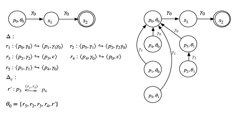
Figure 2: The automata $\mathcal{A}$ (left) and $\mathcal{A}_{pre^{*}}$ (right)

Thus, we can show that:

Theorem 3.

$\mathcal{A}_{pre^{*}}$ recognizes $pre^{*}({L(A)})$.

Before proving this theorem, let us illustrate the construction on 2 examples.

Example 2.

Let us illustrate the procedure by an example. Consider the SM-PDS with control points $P=\{p_{0},p_{1},p_{2},p_{3},p_{4},p_{5}\}$ and $\Delta,\Delta_{c}$ as shown in the left half of Fig. 2. Let $\mathcal{A}$ be the automaton that accepts the set $C=\{(\langle p_{0},\gamma_{0}\gamma_{0}\rangle,\theta_{0})\},$ also shown on the left where $(p_{0},\theta_{0})$ is the initial state and $s_{2}$ is the final state. The result of the algorithm is shown in the right half of Fig. 2. The result is obtained through the following steps:

1. First, we note that $(p_{0},\theta_{0})\xrightarrow{\epsilon}_{T^{\prime}}(p_{0},\theta_{0})$ holds. Since $\langle p_{0},\epsilon\rangle$ occurs on the right hand side of rule $r_{4}$ and $r_{4}\in\theta_{0}$, then Rule $(\alpha_{1})$ adds the transition $(p_{4},\theta_{0})\xrightarrow{\gamma_{0}}(p_{0},\theta_{0})$ to $T^{\prime}$.

2. Now that we have $(p_{4},\theta_{0})\xrightarrow{\gamma_{0}}_{T^{\prime}}(p_{0},\theta_{0})$, since $r_{5}\in\theta_{0}$, Rule $(\alpha_{1})$ adds $(p_{1},\theta_{0})\xrightarrow{\gamma_{1}}(p_{0},\theta_{0})$ to $T^{\prime}$.

3. Since we have $(p_{4},\theta_{0})\xrightarrow{\gamma_{0}}_{T^{\prime}}(p_{0},\theta_{0})$, the self-modifying transition $r^{\prime}\in\theta_{0}$ can be applied. Thus, Rule $(\alpha_{2})$ adds $(p_{3},\theta_{1})\xrightarrow{\gamma_{0}}(p_{0},\theta_{0})$ to $T^{\prime}$ where $\theta_{1}=(\theta_{0}\setminus\{r_{5}\})\cup\{r_{1}\}=\{r_{1},r_{2},r_{3},r_{4},r^{\prime}\}$.

4. Since $(p_{3},\theta_{1})\xrightarrow{\epsilon}(p_{3},\theta_{1})$ and $r_{3}\in\theta_{1}$, Rule $(\alpha_{1})$ adds $(p_{2},\theta_{1})\xrightarrow{\gamma_{2}}(p_{3},\theta_{1})$ to $T^{\prime}$.

5. Then, there is a path $(p_{2},\theta_{1})\xrightarrow{\gamma_{2}}_{T^{\prime}}(p_{3},\theta_{1})\xrightarrow{\gamma_{0}}_{T^{\prime}}(p_{0},\theta_{0})$. Since $\langle p_{2},\gamma_{2}\gamma_{0}\rangle$ occurs on the right hand side of $r_{2}$ and $r_{2}\in\theta_{1}$, then Rule $(\alpha_{1})$ adds the transition $(p_{5},\theta_{1})\xrightarrow{\gamma_{1}}(p_{0},\theta_{0})$ to $T^{\prime}$.

6. No further additions are possible. Thus, the procedure terminates.

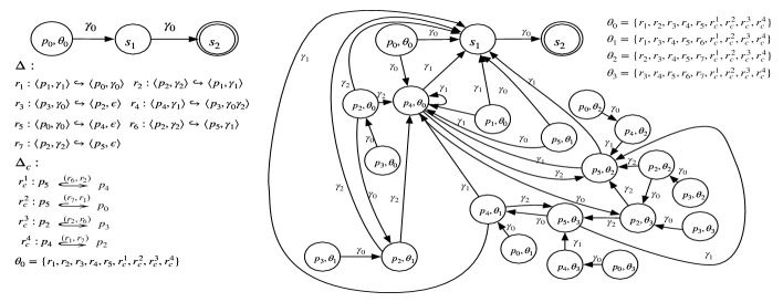
Figure 3: The automata $\mathcal{A}$ (left) and $\mathcal{A}_{pre^{*}}$ (right)

Example 3.

Let us give another example. Consider the SM-PDS with control points $P=\{p_{1},p_{2},p_{3},p_{4},p_{5}\}$ and $\Delta,\Delta_{c}$ as shown in the left half of Fig. 3. Let $\mathcal{A}$ be the automaton that accepts the set $C=\{(\langle p_{0},\gamma_{0}\gamma_{0}\rangle,\theta_{0})\}$ where $(p_{0},\theta_{0})$ is the initial state and $s_{2}$ is the final state as shown on the left. The result $\mathcal{A}_{pre^{*}}$ of the algorithm is on the right half of Fig. 3. The result is obtained through the following steps:

1. Since $(p_{0},\theta_{0})\xrightarrow{\gamma}_{T^{\prime}}s_{1}$ and $r_{1}\in\theta_{0}$, then Rule $(\alpha_{1})$ adds $(p_{1},\theta_{0})\xrightarrow{\gamma_{1}}s_{1}$ to $T^{\prime}$.

2. Since $(p_{1},\theta_{0})\xrightarrow{\gamma_{1}}_{T^{\prime}}s_{1}$ and $r_{2}\in\theta_{0}$, Rule $(\alpha_{1})$ adds the transition $(p_{2},\theta_{0})\xrightarrow{\gamma_{2}}s_{1}$ to $T^{\prime}$.

3. Since $(p_{2},\theta_{0})\xrightarrow{\epsilon}_{T^{\prime}}(p_{2},\theta_{0})$ and $r_{3}\in\theta_{0}$, Rule $(\alpha_{1})$ adds the transition $(p_{3},\theta_{0})\xrightarrow{\gamma_{0}}(p_{2},\theta_{0})$ to $T^{\prime}$.

4. Then, there is a path $(p_{3},\theta_{0})\xrightarrow{\gamma_{0}}_{T^{\prime}}(p_{2},\theta_{0})\xrightarrow{\gamma_{2}}_{T^{\prime}}s_{1}$ and $r_{4}\in\theta_{0}$, Rule $\alpha_{1}$ adds the transition $(p_{4},\theta_{0})\xrightarrow{\gamma_{1}}s_{1}$ to $T^{\prime}$.

5. Because $(p_{4},\theta_{0})\xrightarrow{\epsilon}_{T^{\prime}}(p_{4},\theta_{0})$ and $r_{5}\in\theta_{0}$, Rule $(\alpha_{1})$ adds the transition $(p_{0},\theta_{0})\xrightarrow{\gamma_{0}}(p_{4},\theta_{0})$ to $T^{\prime}$.

6. Since $(p_{0},\theta_{0})\xrightarrow{\gamma_{0}}_{T^{\prime}}(p_{4},\theta_{0})$ and $r_{1}\in\theta_{0}$, Rule $(\alpha_{1})$ adds the transition $(p_{1},\theta_{0})\xrightarrow{\gamma_{1}}(p_{4},\theta_{0})$ to $T^{\prime}$. Then, since $r_{2}\in\theta_{0}$, Rule $(\alpha_{1})$ adds the transition $(p_{2},\theta_{0})\xrightarrow{\gamma_{2}}(p_{4},\theta_{0})$ to $T^{\prime}$.

7. Since there is a path $(p_{3},\theta_{0})\xrightarrow{\gamma_{0}}_{T^{\prime}}(p_{2},\theta_{0})\xrightarrow{\gamma_{2}}_{T^{\prime}}(p_{4},\theta_{0})$ and $r_{4}\in\theta_{0}$, Rule $(\alpha_{1})$ adds $(p_{4},\theta_{0})\xrightarrow{\gamma_{1}}(p_{4},\theta_{0})$ to $T^{\prime}$.

8. Since $(p_{4},\theta_{0})\xrightarrow{\gamma_{1}}_{T^{\prime}}s_{1},(p_{4},\theta_{0})\xrightarrow{\gamma_{1}}_{T^{\prime}}(p_{4},\theta_{0})$ and $r_{c}^{1},r_{2}\in\theta_{0}$, Rule $(\alpha_{2})$ adds $(p_{5},\theta_{1})\xrightarrow{\gamma_{1}}s_{1}$ and $(p_{5},\theta_{1})\xrightarrow{\gamma_{1}}(p_{4},\theta_{0})$ to $T^{\prime}$ where $\theta_{1}=(\theta_{0}\setminus\{r_{2}\})\cup r_{6}=\{r_{1},r_{3},r_{4},r_{5},r_{6},r_{c}^{1},r_{c}^{2},r_{c}^{3},r_{c}^{4}\}$. For the same reason, since $(p_{0},\theta_{0})\xrightarrow{\gamma_{0}}_{T^{\prime}}(p_{4},\theta_{0})$, $(p_{0},\theta_{0})\xrightarrow{\gamma}_{T^{\prime}}s_{1}$ and $r_{1},\in\theta_{1}$, $r_{c}^{2}\in\theta_{0}$, Rule $(\alpha_{2})$ adds the transitions $(p_{5},\theta_{2})\xrightarrow{\gamma_{0}}(p_{4},\theta_{0})$ and $(p_{5},\theta_{2})\xrightarrow{\gamma_{0}}s_{1}$ to $T^{\prime}$ where $\theta_{2}=(\theta_{0}\setminus\{r_{1}\})\cup\{r_{7}\}=\{r_{2},r_{3},r_{4},r_{5},r_{7},r_{c}^{1},r_{c}^{2},r_{c}^{3},r_{c}^{4}\}.$

9. Since $(p_{5},\theta_{1})\xrightarrow{\gamma_{1}}_{T^{\prime}}s_{1}$, $(p_{5},\theta_{1})\xrightarrow{\gamma_{1}}_{T^{\prime}}(p_{4},\theta_{0})$ and $r_{6}\in\theta_{1}$, Rule $(\alpha_{1})$ adds the transitions $(p_{2},\theta_{1})\xrightarrow{\gamma_{2}}s_{1}$ and $(p_{2},\theta_{1})\xrightarrow{\gamma_{2}}(p_{4},\theta_{0})$ to $T^{\prime}$.

10. Since $(p_{2},\theta_{1})\xrightarrow{\epsilon}_{T^{\prime}}(p_{2},\theta_{1})$ and $r_{3}\in\theta_{1}$, Rule $(\alpha_{1})$ adds $(p_{3},\theta_{1})\xrightarrow{\gamma_{0}}(p_{2},\theta_{1})$.

11. Because there are paths $(p_{3},\theta_{1})\xrightarrow{\gamma_{0}}_{T^{\prime}}(p_{2},\theta_{1})\xrightarrow{\gamma_{2}}_{T^{\prime}}(p_{4},\theta_{0})$ and $(p_{3},\theta_{1})\xrightarrow{\gamma_{0}}_{T^{\prime}}(p_{2},\theta_{1})\xrightarrow{\gamma_{2}}_{T^{\prime}}s_{1}$, Rule $(\alpha_{1})$ adds the transitions $(p_{4},\theta_{1})\xrightarrow{\gamma_{1}}(p_{4},\theta_{0})$ and $(p_{4},\theta_{1})\xrightarrow{\gamma_{1}}s_{1}$ to $T^{\prime}$.

12. Since $(p_{4},\theta_{0})\xrightarrow{\epsilon}_{T^{\prime}}(p_{4},\theta_{0})$ and $r_{5}\in\theta_{1}$, Rule $(\alpha_{1})$ adds $(p_{0},\theta_{1})\xrightarrow{\gamma_{0}}(p_{4},\theta_{1})$.

13. Now we have $(p_{0},\theta_{1})\xrightarrow{\gamma_{0}}_{T^{\prime}}(p_{4},\theta_{1})$ and $r_{c}^{2},r_{1}\in\theta_{1}$, Rule $(\alpha_{2})$ adds the transition $(p_{5},\theta_{3})\xrightarrow{\gamma_{0}}(p_{4},\theta_{1})$ to $T^{\prime}$ where $\theta_{3}=\{r_{3},r_{4},r_{5},r_{6},r_{7},r_{c}^{1},r_{c}^{2},r_{c}^{3},r_{c}^{4}\}$. For the same reason, since $(p_{3},\theta_{1})\xrightarrow{\gamma_{0}}(p_{2},\theta_{1})$ and $r_{c}^{3},r_{6}\in\theta_{1}$, Rule $\alpha_{2}$ adds the transition $(p_{2},\theta_{0})\xrightarrow{\gamma_{0}}(p_{2},\theta_{1})$ to $T^{\prime}$ because $\theta_{0}=(\theta_{1}\setminus\{r_{6}\})\cup\{r_{2}\}$.

14. Since $(p_{5},\theta_{3})\xrightarrow{\epsilon}_{T^{\prime}}(p_{5},\theta_{3})$ and $r_{7}\in\theta_{3}$, Rule $(\alpha_{1})$ adds the transition $(p_{2},\theta_{3})\xrightarrow{\gamma_{2}}(p_{5},\theta_{3})$ to $T^{\prime}$.

15. Because $(p_{2},\theta_{3})\xrightarrow{\epsilon}_{T^{\prime}}(p_{2},\theta_{3})$ and $r_{3}\in\theta_{3}$, Rule ($\alpha_{1}$) adds the transition $(p_{3},\theta_{3})\xrightarrow{\gamma_{0}}(p_{2},\theta_{3})$ to $T^{\prime}$. Then, since there is a path $(p_{3},\theta_{3})\xrightarrow{\gamma_{0}}_{T^{\prime}}(p_{2},\theta_{3})\xrightarrow{\gamma_{2}}_{T^{\prime}}(p_{5},\theta_{3})$ and $r_{4}\in\theta_{3}$, Rule $(\alpha_{1})$ adds the transition $(p_{4},\theta_{3})\xrightarrow{\gamma_{1}}(p_{5},\theta_{3})$ to $T^{\prime}$. Then, since $r_{5}\in\theta_{3}$, Rule $(\alpha_{1})$ adds the transition $(p_{0},\theta_{3})\xrightarrow{\gamma_{0}}(p_{4},\theta_{3})$ to $T^{\prime}$.

16. Since $(p_{3},\theta_{3})\xrightarrow{\gamma_{0}}_{T^{\prime}}(p_{2},\theta_{3})$ and $r_{c}^{3}\in\theta_{3}$, Rule $(\alpha_{2})$ adds the transition $(p_{2},\theta_{2})\xrightarrow{\gamma_{0}}_{T^{\prime}}(p_{2},\theta_{3})$ to $T^{\prime}$ where $(\theta_{3}\setminus\{r_{6}\})\cup\{r_{2}\}=\theta_{2}$. Meanwhile, since $(p_{2},\theta_{3})\xrightarrow{\gamma_{2}}(p_{5},\theta_{3})$ and $r_{c}^{4},r_{7}\in\theta_{3}$, Rule $(\alpha_{2})$ adds the transition $(p_{4},\theta_{1})\xrightarrow{\gamma_{2}}(p_{5},\theta_{3})$ to $T^{\prime}$ where $(\theta_{3}\setminus\{r_{7}\})\cup\{r_{1}\}=\theta_{1}$.

17. Because $r_{7}\in\theta_{2}$ and $(p_{5},\theta_{2})\xrightarrow{\epsilon}_{T^{\prime}}(p_{5},\theta_{2})$, Rule ($\alpha_{1}$) adds the transition $(p_{2},\theta_{2})\xrightarrow{\gamma_{2}}(p_{5},\theta_{2})$ to $T^{\prime}$.

18. Since $(p_{2},\theta_{2})\xrightarrow{\epsilon}_{T^{\prime}}(p_{2},\theta_{2})$ and $r_{3}\in\theta_{2}$, Rule $(\alpha_{1})$ adds $(p_{3},\theta_{2})\xrightarrow{\gamma_{0}}_{T^{\prime}}(p_{2},\theta_{2})$ to $T^{\prime}$. Then, there is a path $(p_{3},\theta_{2})\xrightarrow{\gamma_{0}\gamma_{2}}_{T^{\prime}}^{*}(p_{5},\theta_{2})$, since $r_{4}\in\theta_{2}$, Rule $(\alpha_{1})$ adds the transition $(p_{4},\theta_{2})\xrightarrow{\gamma_{1}}_{T^{\prime}}(p_{5},\theta_{2})$ to $T^{\prime}$. Then, since $(p_{5},\theta_{2})\xrightarrow{\epsilon}_{T^{\prime}}(p_{5},\theta_{2})$ and $r_{5}\in\theta_{2}$, Rule $(\alpha_{1})$ adds the transition $(p_{0},\theta_{2})\xrightarrow{\gamma_{0}}(p_{4},\theta_{2})$ to $T^{\prime}$.

19. Now we have $(p_{2},\theta_{2})\xrightarrow{\gamma_{2}}_{T^{\prime}}(p_{5},\theta_{2})$ and $(p_{2},\theta_{2})\xrightarrow{\gamma_{0}}_{T^{\prime}}(p_{2},\theta_{3})$, since $r_{c}^{4},r_{7}\in\theta_{2}$, Rule $\alpha_{2}$ adds the transitions $(p_{4},\theta_{0})\xrightarrow{\gamma_{2}}(p_{5},\theta_{2})$ and $(p_{4},\theta_{0})\xrightarrow{\gamma_{0}}(p_{2},\theta_{3})$ to $T^{\prime}$ where $(\theta_{2}\setminus\{r_{7}\}\cup)\{r_{1}\}=\theta_{0}.$

20. Since $(p_{4},\theta_{2})\xrightarrow{\gamma_{1}}_{T^{\prime}}(p_{5},\theta_{2})$ and $r_{2},r_{c}^{1}\in\theta_{2}$, Rule $(\alpha_{2})$ adds the transition $(p_{5},\theta_{3})\xrightarrow{\gamma_{1}}(p_{5},\theta_{2})$ to $T^{\prime}$ where $(\theta_{2}\setminus\{r_{2}\})\cup\{r_{6}\}=\theta_{3}.$

21. Since $(p_{5},\theta_{3})\xrightarrow{\gamma_{1}}_{T^{\prime}}(p_{5},\theta_{2})$ and $r_{6}\in\theta_{3}$, Rule $(\alpha_{1})$ adds the transition $(p_{2},\theta_{3})\xrightarrow{\gamma_{2}}(p_{5},\theta_{2})$ to $T^{\prime}$.

22. No further additions are possible, so the procedure terminates.

V-A Proof of Theorem 3

Let us now prove Theorem 3. To prove this theorem, we first introduce the following lemma.

Lemma 1.

For every configuration $(\langle p,w\rangle,\theta_{0})\in L(A)$, if $(\langle p^{\prime},w^{\prime}\rangle,\theta)\Rightarrow_{\mathcal{P}}^{*}(\langle p,w\rangle,\theta_{0})$, then $(p^{\prime},\theta)\xrightarrow{w^{\prime}}_{T^{\prime}}q$ for some final state $q$ of $\mathcal{A}_{pre^{*}}$.

Proof:  Assume $(\langle p^{\prime},w^{\prime}\rangle,\theta)\stackrel{{\scriptstyle i}}{{\Rightarrow}}_{\mathcal{P}}(\langle p,w\rangle,\theta_{0})$. We proceed by induction on $i$.

Basis. $i=0$. Then $\theta=\theta_{0},p^{\prime}=p$ and $w=w^{\prime}$. Since $(\langle p,w\rangle,\theta_{0})\in L(A)$, we have $(p,\theta_{0})\xrightarrow{w}_{T^{\prime}}q$ always holds for some final state $q$ i.e. $(p^{\prime},\theta)\xrightarrow{w^{\prime}}_{T^{\prime}}q$ holds.

Step. $i>0$. Then there exists a configuration $(\langle p^{\prime\prime},u\rangle,\theta^{\prime\prime})$ such that

$$(\langle p^{\prime},w^{\prime}\rangle,\theta)\Rightarrow_{\mathcal{P}}(\langle p^{\prime\prime},u\rangle,\theta^{\prime\prime})\stackrel{{\scriptstyle i-1}}{{\Rightarrow}}_{\mathcal{P}}(\langle p,w\rangle,\theta_{0})$$

We apply the induction hypothesis to $(\langle p^{\prime\prime},u\rangle,\theta^{\prime\prime})\stackrel{{\scriptstyle i-1}}{{\Rightarrow}}(\langle p,w\rangle,\theta_{0})$, and obtain $(p^{\prime\prime},\theta^{\prime\prime})\mathop{{\hbox{{$\mathrel{\mathop{\hbox to11.00722pt{\rightarrowfill}}\limits^{u}}$}}}}_{T^{\prime}}q$ for $q\in F$.

Let $w_{1},u_{1}\in\Gamma^{*},\gamma^{\prime}\in\Gamma$ be such that $w^{\prime}=\gamma^{\prime}w_{1}$, $u=u_{1}w_{1}$. Let $q^{\prime}$ be a state of $\mathcal{A}_{pre^{*}}$ s.t.

$$(p^{\prime\prime},\theta^{\prime\prime}){\mathop{{\hbox{{$\mathrel{\mathop{\hbox to13.00722pt{\rightarrowfill}}\limits^{u_{1}}}$}}}}}_{T^{\prime}}q^{\prime}{\mathop{{\hbox{{$\mathrel{\mathop{\hbox to14.19978pt{\rightarrowfill}}\limits^{w_{1}}}$}}}}}_{T^{\prime}}q$$ (1)

There are two cases depending on which rule is applied to get $(\langle p^{\prime},w^{\prime}\rangle,\theta)\Rightarrow(\langle p^{\prime\prime},u\rangle,\theta^{\prime\prime})$.

1. Case $(\langle p^{\prime},w^{\prime}\rangle,\theta)\Rightarrow(\langle p^{\prime\prime},u\rangle,\theta^{\prime\prime})$ is obtained by a rule of the form: $\langle p^{\prime},\gamma^{\prime}\rangle\hookrightarrow\langle p^{\prime\prime},u_{1}\rangle\in\Delta$. In this case, $\theta^{\prime\prime}=\theta.$ By the saturation rule $\alpha_{1}$, we have

   $$(p^{\prime},\theta^{\prime\prime}){\mathop{{\hbox{{$\mathrel{\mathop{\hbox to11.72412pt{\rightarrowfill}}\limits^{\gamma^{\prime}}}$}}}}}_{T^{\prime}}q^{\prime}$$ (2)

   Putting (1) and (2) together, we can obtain that

   $$\pi=(p^{\prime},\theta^{\prime\prime}){\mathop{{\hbox{{$\mathrel{\mathop{\hbox to11.72412pt{\rightarrowfill}}\limits^{\gamma^{\prime}}}$}}}}}_{T^{\prime}}q^{\prime}{\mathop{{\hbox{{$\mathrel{\mathop{\hbox to14.19978pt{\rightarrowfill}}\limits^{w_{1}}}$}}}}}_{T^{\prime}}q$$ (3)

   Thus, $(p^{\prime},\theta^{\prime\prime})\mathop{{\hbox{{$\mathrel{\mathop{\hbox to18.92389pt{\rightarrowfill}}\limits^{\gamma^{\prime}w_{1}}}$}}}}_{T^{\prime}}q$ i.e. $(p^{\prime},\theta)\mathop{{\hbox{{$\mathrel{\mathop{\hbox to13.29977pt{\rightarrowfill}}\limits^{w^{\prime}}}$}}}}q$ for some final state $q\in F$.

2. Case $(\langle p^{\prime},w^{\prime}\rangle,\theta)\Rightarrow(\langle p^{\prime\prime},u\rangle,\theta^{\prime\prime})$ is obtained by a rule of the form $p^{\prime}\stackrel{{\scriptstyle(r_{1},r_{2})}}{{\lhook\joinrel\relbar\joinrel\relbar\joinrel\relbar\joinrel\relbar\joinrel\rightarrow}}p^{\prime\prime}\in\Delta_{c}$. I.e $\theta^{\prime\prime}\neq\theta.$ In this case, $u_{1}=\gamma^{\prime}$. By the saturation rule $\alpha_{2}$, we obtain that

   $$(p^{\prime},\theta){\mathop{{\hbox{{$\mathrel{\mathop{\hbox to11.72412pt{\rightarrowfill}}\limits^{\gamma^{\prime}}}$}}}}}_{T^{\prime}}q^{\prime}\text{ where }\theta^{\prime\prime}=\theta\backslash\{r_{1}\}\cup\{r_{2}\}.$$ (4)

   Putting (1) and (4) together, we have the following path

   $$(p^{\prime},\theta){\mathop{{\hbox{{$\mathrel{\mathop{\hbox to11.72412pt{\rightarrowfill}}\limits^{\gamma^{\prime}}}$}}}}}_{T^{\prime}}q^{\prime}{\mathop{{\hbox{{$\mathrel{\mathop{\hbox to14.19978pt{\rightarrowfill}}\limits^{w_{1}}}$}}}}}_{T^{\prime}}q.\text{ I.e. }(p^{\prime},\theta){\mathop{{\hbox{{$\mathrel{\mathop{\hbox to13.29977pt{\rightarrowfill}}\limits^{w^{\prime}}}$}}}}}_{T^{\prime}}q\text{ for }q\in F$$ (5)

$\;\;\Box$

Lemma 2.

If a path $\pi=(p,\theta)\xrightarrow{w}_{T^{\prime}}q$ for $\theta\subseteq\Delta\cup\Delta_{c}$ is in $\mathcal{A}_{pre^{*}}$, then

1. $(\langle p,w\rangle,\theta)\Rightarrow^{*}(\langle p^{\prime},w^{\prime}\rangle,\theta_{0})$ holds for a configuration $(\langle p^{\prime},w^{\prime}\rangle,\theta_{0})$ s.t. $(p^{\prime},\theta_{0}){\mathop{{\hbox{{$\mathrel{\mathop{\hbox to13.29977pt{\rightarrowfill}}\limits^{w^{\prime}}}$}}}}}_{T}q$ in the initial $\mathcal{P}$-automaton $\mathcal{A}$;

2. Moreover, if $q$ is an initial state i.e. in the form $(p,\theta)$, then $w^{\prime}=\epsilon$.

Proof:  Let $\mathcal{A}_{pre^{*}}=(Q,\Gamma,T,P,F)$ be the $\mathcal{P}$-automaton computed by the saturation procedure. In this proof, we use $\xlongrightarrow[i]{}_{T^{\prime}}$ to denote the transition relation of $\mathcal{A}_{pre^{*}}$ obtained after adding $i$-transitions using the saturation procedure. In particular, since initially $\mathcal{A}_{pre^{*}}=\mathcal{A}$, $\mathcal{A}_{pre^{*}}$ contains the path $(p^{\prime},\theta_{0})\xlongrightarrow{w^{\prime}}_{T}q$ where $(\langle p^{\prime},w^{\prime}\rangle,\theta_{0})\in L(A)$, then we write $(p^{\prime},\theta_{0})\xlongrightarrow[0]{w^{\prime}}_{T}q$.

Let $i$ be an index such that $\pi=(p,\theta)\xlongrightarrow[i]{w}_{T^{\prime}}q$ holds. We shall prove (I) by induction on $i$. Statement (II) then follows immediately from the fact that initial states have no incoming transitions in $\mathcal{A}$.

Basis. $i=0$. Since $(\langle p,w\rangle,\theta)\Rightarrow^{*}(\langle p,w\rangle,\theta)$ always holds, take then $p=p^{\prime},w=w^{\prime}$ and $\theta_{0}=\theta$.

Step. $i>0$. Let $t=((p_{1},\theta_{1}),\gamma,q^{\prime})$ be the $i$-th transition added to $\mathcal{A}_{pre^{*}}$ and $j$ be the number of times that $t$ is used in the path $(p,\theta){\xlongrightarrow[i]{w}}_{T^{\prime}}q$. The proof is by induction on $j$. If $j=0$, then we have $(p,\theta){\xlongrightarrow[i-1]{w}}_{T^{\prime}}q$ in the automaton, and we apply the induction hypothesis (induction on $i$) then we obtain $(\langle p,w\rangle,\theta)\Rightarrow^{*}(\langle p^{\prime},w^{\prime}\rangle,\theta_{0})$ for a configuration $(\langle p^{\prime},w^{\prime}\rangle,\theta_{0})$ s.t. $(p^{\prime},\theta_{0}){\mathop{{\hbox{{$\mathrel{\mathop{\hbox to13.29977pt{\rightarrowfill}}\limits^{w^{\prime}}}$}}}}}_{T}q$ in the initial $\mathcal{P}$-automaton $\mathcal{A}$. So assume that $j>0$. Then, there exist $u$ and $v$ such that $w=u\gamma v$ and

$$(p,\theta){\xlongrightarrow[i-1]{u}}_{T^{\prime}}(p_{1},\theta_{1}){\xlongrightarrow[i]{\gamma}}_{T^{\prime}}q^{\prime}{\xlongrightarrow[i]{v}}_{T^{\prime}}q$$ (1)

The application of the induction hypothesis (induction on $i$) to $(p,\theta)\xlongrightarrow[i-1]{u}_{T^{\prime}}(p_{1},\theta_{1})$ (notice that $(p_{1},\theta_{1})$ is an initial state) gives that

$$(\langle p,u\rangle,\theta)\Rightarrow^{*}(\langle p_{1},\epsilon\rangle,\theta_{1})$$ (2)

There are 2 cases depending on whether transition $t$ was added by saturation rule $\alpha_{1}$ or $\alpha_{2}$.

1. Case $t$ was added by rule $\alpha_{1}$: There exist $p_{2}\in P$ and $w_{2}\in\Gamma^{*}$ such that

   $$r=\langle p_{1},\gamma\rangle\hookrightarrow\langle p_{2},w_{2}\rangle\in\Delta\cap\theta_{1}$$ (3)

   and $\mathcal{A}_{pre^{*}}$ contains the following path:

   $$\pi^{\prime}=(p_{2},\theta_{1})\xlongrightarrow[i-1]{w_{2}}_{T^{\prime}}q^{\prime}\xlongrightarrow[i]{v}_{T^{\prime}}q$$ (4)

   Applying the transition rule $r$ gets that

   $$(\langle p_{1},\gamma v\rangle,\theta_{1})\Rightarrow(\langle p_{2},w_{2}v\rangle,\theta_{1})$$ (5)

   By induction on $j$ (since transition $t$ is used $j-1$ times in $\pi^{\prime}$), we get from (4) that

   $$(\langle p_{2},w_{2}v\rangle,\theta_{1})\Rightarrow^{*}(\langle p^{\prime},w^{\prime}\rangle,\theta_{0})\text{ s.t. }(p^{\prime},\theta_{0}){\mathop{{\hbox{{$\mathrel{\mathop{\hbox to13.29977pt{\rightarrowfill}}\limits^{w^{\prime}}}$}}}}}_{T^{\prime}}q$$ (6)

   $$\text{ in the initial }\mathcal{P}\text{-automaton }\mathcal{A}$$

   Putting (2) ,(5) and (6) together, we can obtain that

   $$(\langle p,w\rangle,\theta)=(\langle p,u\gamma v\rangle,\theta)\Rightarrow^{*}(\langle p_{1},\gamma v\rangle,\theta_{1})\Rightarrow$$

   $$(\langle p_{2},w_{2}v\rangle,\theta_{1})\Rightarrow^{*}(\langle p^{\prime},w^{\prime}\rangle,\theta_{0})$$

   such that $(p^{\prime},\theta_{0}){\mathop{{\hbox{{$\mathrel{\mathop{\hbox to13.29977pt{\rightarrowfill}}\limits^{w^{\prime}}}$}}}}}_{T}q$ in the initial $\mathcal{P}$-automaton $\mathcal{A}$

2. Case $t$ was added by rule $\alpha_{2}:$ there exist $p_{2}\in P$ and $\theta^{\prime\prime}\subseteq\Delta\cup\Delta_{c}$ such that

   $$p_{1}\stackrel{{\scriptstyle(r_{1},r_{2})}}{{\lhook\joinrel\relbar\joinrel\relbar\joinrel\relbar\joinrel\relbar\joinrel\rightarrow}}p_{2}\in\Delta_{c}\cap\theta^{\prime\prime},\theta^{\prime\prime}=(\theta_{1}\backslash\{r_{1}\})\cup\{r_{2}\}$$ (7)

   and the following path in the current automaton ( self-modifying rule won’t change the stack) with $r\in\theta^{\prime\prime}:$

   $$(p_{2},\theta^{\prime\prime}){\xrightarrow[i-1]{\gamma}_{T^{\prime}}}q^{\prime}\xlongrightarrow[i]{v}_{T^{\prime}}q$$ (8)

   Applying the transition rule, we can get from (7) that

   $$(\langle p_{1},\gamma v\rangle,\theta_{1})\Rightarrow(\langle p_{2},\gamma v\rangle,\theta^{\prime\prime})$$ (9)

   We can apply the induction hypothesis (on $j$) to (8), and obtain

   $$(\langle p_{2},\gamma v\rangle,\theta^{\prime\prime})\Rightarrow^{*}(\langle p^{\prime},w^{\prime}\rangle,\theta_{0})\text{ s.t. }(p^{\prime},\theta_{0}){\mathop{{\hbox{{$\mathrel{\mathop{\hbox to13.29977pt{\rightarrowfill}}\limits^{w^{\prime}}}$}}}}}_{T}q$$ (10)

   $$\text{ in the initial }\mathcal{P}\text{-automaton }\mathcal{A}$$

   From (2),(9) and (10), we get

   $$(\langle p,w\rangle,\theta)=(\langle p,u\gamma v\rangle,\theta)\Rightarrow^{*}(\langle p_{1},\gamma v\rangle,\theta_{1})\Rightarrow$$

   $$(\langle p_{2},\gamma v\rangle,\theta^{\prime\prime})\Rightarrow^{*}(\langle p^{\prime},w^{\prime}\rangle,\theta_{0})$$

   such that $(p^{\prime},\theta_{0}){\mathop{{\hbox{{$\mathrel{\mathop{\hbox to13.29977pt{\rightarrowfill}}\limits^{w^{\prime}}}$}}}}}_{T}q$ in the initial $\mathcal{P}$-automaton $\mathcal{A}$.

$\;\;\Box$

Then, we can prove Theorem 3:

Proof:  Let $(\langle p,w\rangle,\theta)$ be a configuration of $pre^{*}(L(A))$. Then $(\langle p,w\rangle,\theta)\Rightarrow^{*}(\langle p^{\prime},w^{\prime}\rangle,\theta_{0})$ for a configuration $(\langle p^{\prime},w^{\prime}\rangle,\theta_{0})$ s.t. $(p^{\prime},\theta_{0}){\mathop{{\hbox{{$\mathrel{\mathop{\hbox to13.29977pt{\rightarrowfill}}\limits^{w^{\prime}}}$}}}}}_{T^{\prime}}q$ is a path in $\mathcal{A}$ for $q\in F$. By lemma 1, we can obtain that there exists a path $(p,\theta)\xrightarrow{w}_{T^{\prime}}q$ for some final state $q$ of $\mathcal{A}_{pre^{*}}$. So $(\langle p,w\rangle,\theta)$ is recognized by $\mathcal{A}_{pre^{*}}$.

Conversely, let $(\langle p,w\rangle,\theta)$ be a configuration accepted by $\mathcal{A}_{pre^{*}}$ i.e. there exists a path $(p,\theta)\xrightarrow{w}_{T^{\prime}}q$ in $\mathcal{A}_{pre^{*}}$ for some final state $q\in F$. By lemma 2, there exists a configuration $(\langle p^{\prime},w^{\prime}\rangle,\theta_{0})$ s.t. there exist a path $(p^{\prime},\theta_{0})\xrightarrow{w^{\prime}}_{T}q$ in the initial automaton $\mathcal{A}$ and $(\langle p,w\rangle,\theta)\Rightarrow^{*}(\langle p^{\prime},w^{\prime}\rangle,\theta_{0})$. Because $q$ is a final state, we have $(\langle p^{\prime},w^{\prime}\rangle,\theta_{0})\in L(A)$ i.e. $(\langle p,w\rangle,\theta)\in pre^{*}(L(A))$.

$\;\;\Box$

VI Efficient computation of $post^{*}$ images

Let $\mathcal{P}=(P,\Gamma,\Delta,\Delta_{c})$ be a SM-PDS, and let $\mathcal{A}=(Q,\Gamma,T,P,F)$ be a $\mathcal{P}$-automaton that represents a regular set of configurations $\mathcal{C}$ ( $\mathcal{C}=L(\mathcal{A})$). Similarly, it is not optimal to compute $post^{*}(\mathcal{C})$ using the translations of Sections II-B and II-C to compute equivalent PDSs or symbolic PDSs, and then apply the algorithms of [EHRS00, Sch02]. We present in this section a direct and efficient algorithm that computes $post^{*}(\mathcal{C})$. We assume w.l.o.g. that $\mathcal{A}$ has no transitions leading to an initial state. Moreover, we assume that the rules of $\Delta$ are of the form $\langle p,\gamma\rangle\hookrightarrow\langle p^{\prime},w\rangle$, where $|w|\leq 2$. This is not a restriction, indeed, a rule of the form $\langle p,\gamma\rangle\hookrightarrow\langle p^{\prime},\gamma_{1}\cdots\gamma_{n}\rangle$, $n>2$ can be replaced by the following rules:

• $\langle p,\gamma\rangle\hookrightarrow\langle p_{1},a_{1}\gamma_{n}\rangle$

• $\langle p_{1},a_{1}\rangle\hookrightarrow\langle p_{2},a_{2}\gamma_{n-1}\rangle$

• $\langle p_{2},a_{2}\rangle\hookrightarrow\langle p_{3},a_{3}\gamma_{n-2}\rangle$

• $\cdots$,

• $\langle p_{n-2},a_{n-2}\rangle\hookrightarrow\langle{p^{\prime}},\gamma_{1}\gamma_{2}\rangle$

As previously, the construction of $\mathcal{A}_{post^{*}}$ consists in adding iteratively new transitions to the automaton $\mathcal{A}$ according to saturation rules (reflecting the forward application of the transition rules in the system). We define $\mathcal{A}_{post^{*}}$ to be the $\mathcal{P}$-automaton $({Q^{\prime}},\Gamma,T^{\prime},P,F)$, where $T^{\prime}$ is computed using the following saturation rules and $Q^{\prime}$ is the smallest set s.t. $Q\subseteq Q^{\prime}$ and for every $r=\langle p,\gamma\rangle\hookrightarrow\langle p^{\prime},\gamma_{1}\gamma_{2}\rangle\in\Delta,q_{p^{\prime}\gamma_{1}}^{\theta}\in Q^{\prime}$ where $q_{p^{\prime}\gamma_{1}}^{\theta}$ is the new state labelled with $p^{\prime},\gamma_{1}$ and $\theta$: initially $T^{\prime}=T$;

1. If $r=\langle p,\gamma\rangle\hookrightarrow\langle p^{\prime},\epsilon\rangle\in\Delta$ and there exists in $T^{\prime}$ a path $\pi=(p,\theta)\mathop{{\hbox{{$\mathrel{\mathop{\hbox to10.62413pt{\rightarrowfill}}\limits^{\gamma}}$}}}}_{T^{\prime}}q$ with $r\in\theta$, then add $((p^{\prime},\theta),\epsilon,q)$ to $T^{\prime}$.

2. If $r=\langle p,\gamma\rangle\hookrightarrow\langle p^{\prime},\gamma^{\prime}\rangle\in\Delta$ and there exists in $T^{\prime}$ a path $\pi=(p,\theta)\mathop{{\hbox{{$\mathrel{\mathop{\hbox to10.62413pt{\rightarrowfill}}\limits^{\gamma}}$}}}}_{T^{\prime}}q$ with $r\in\theta$, then add $((p^{\prime},\theta),\gamma^{\prime},q)$ to $T^{\prime}$.

3. If $r=\langle p,\gamma\rangle\hookrightarrow\langle p^{\prime},\gamma_{1}\gamma_{2}\rangle\in\Delta$ and there exists in $T^{\prime}$ a path $\pi=(p,\theta)\mathop{{\hbox{{$\mathrel{\mathop{\hbox to10.62413pt{\rightarrowfill}}\limits^{\gamma}}$}}}}_{T^{\prime}}q$ with $r\in\theta$. Add $t^{\prime}=((p^{\prime},\theta),\gamma_{1},q_{p^{\prime}\gamma_{1}}^{\theta})$ and $t^{\prime\prime}=(q_{p^{\prime}\gamma_{1}}^{\theta},\gamma_{2},q)$ to $T^{\prime}$.

4. if $r=p\stackrel{{\scriptstyle(r_{1},r_{2})}}{{\lhook\joinrel\relbar\joinrel\relbar\joinrel\relbar\joinrel\relbar\joinrel\rightarrow}}p^{\prime}\in\Delta_{c}$ and there exists in $T^{\prime}$ a path $\pi=(p,\theta)\mathop{{\hbox{{$\mathrel{\mathop{\hbox to10.62413pt{\rightarrowfill}}\limits^{\gamma}}$}}}}_{T^{\prime}}q$, where $\gamma\in\Gamma$ with $r\in\theta$, and $r_{1}\in\theta$, then add $t^{\prime}=((p^{\prime},\theta^{\prime}),\gamma,q)$ where $\theta^{\prime}=(\theta\setminus\{r_{1}\})\cup\{r_{2}\}\}$.

The procedure above terminates since there is a finite number of states and phases.

Let us explain intuitively the role of the saturation rules above. Consider a path in the automaton of the form $(p,\theta)\mathop{{\hbox{{$\mathrel{\mathop{\hbox to10.62413pt{\rightarrowfill}}\limits^{\gamma}}$}}}}_{T^{\prime}}q\mathop{{\hbox{{$\mathrel{\mathop{\hbox to13.29977pt{\rightarrowfill}}\limits^{w^{\prime}}}$}}}}_{T^{\prime}}q_{F}$, where $q_{F}\in F$. This means, by definition of $\mathcal{P}$-automata, that the configuration $c=(\langle p,\gamma w^{\prime}\rangle,\theta)$ is accepted by $\mathcal{A}_{post^{*}}$.

Let $r=\langle p,\gamma\rangle\hookrightarrow\langle p^{\prime},\epsilon\rangle\in\Delta$. If $r$ is in $\theta$, then the configuration $c^{\prime}=(\langle p^{\prime},w^{\prime}\rangle,\theta)$ is a successor of $c$. Therefore, it should be added to $\mathcal{A}_{post^{*}}$. This configuration is accepted by the run $(p^{\prime},\theta)\mathop{{\hbox{{$\mathrel{\mathop{\hbox to9.84134pt{\rightarrowfill}}\limits^{\epsilon}}$}}}}_{T^{\prime}}q\mathop{{\hbox{{$\mathrel{\mathop{\hbox to13.29977pt{\rightarrowfill}}\limits^{w^{\prime}}}$}}}}_{T^{\prime}}q_{F}$ added by rules ($\beta_{1}$).

If $\theta$ contains the rule $r=\langle p,\gamma\rangle\hookrightarrow\langle p^{\prime},\gamma^{\prime}\rangle\in\Delta$, then the configuration $c^{\prime}=(\langle p^{\prime},\gamma^{\prime}w^{\prime}\rangle,\theta)$ is a successor of $c$. Therefore, it should be added to $\mathcal{A}_{post^{*}}$. This configuration is accepted by the run $(p^{\prime},\theta)\mathop{{\hbox{{$\mathrel{\mathop{\hbox to11.72412pt{\rightarrowfill}}\limits^{\gamma^{\prime}}}$}}}}_{T^{\prime}}q\mathop{{\hbox{{$\mathrel{\mathop{\hbox to13.29977pt{\rightarrowfill}}\limits^{w^{\prime}}}$}}}}_{T^{\prime}}q_{F}$ added by rules ($\beta_{2}$).

If $r=\langle p,\gamma\rangle\hookrightarrow\langle p^{\prime},\gamma_{1}\gamma_{2}\rangle\in\Delta$ is in $\theta$, then the configuration $c^{\prime}=(\langle p^{\prime},\gamma_{1}\gamma_{2}w^{\prime}\rangle,\theta)$ is a successor of $c$. Therefore, it should be added to $\mathcal{A}_{post^{*}}$. This configuration is accepted by the run $(p^{\prime},\theta)\mathop{{\hbox{{$\mathrel{\mathop{\hbox to12.62413pt{\rightarrowfill}}\limits^{\gamma_{1}}}$}}}}_{T^{\prime}}q_{p^{\prime}\gamma_{1}}^{\theta}\mathop{{\hbox{{$\mathrel{\mathop{\hbox to12.62413pt{\rightarrowfill}}\limits^{\gamma_{2}}}$}}}}_{T^{\prime}}q\mathop{{\hbox{{$\mathrel{\mathop{\hbox to13.29977pt{\rightarrowfill}}\limits^{w^{\prime}}}$}}}}_{T^{\prime}}q_{F}$ added by rules ($\beta_{3}$).

Rule ($\beta_{4}$) deals with modifying rules: Let $r=p\stackrel{{\scriptstyle(r_{1},r_{2})}}{{\lhook\joinrel\relbar\joinrel\relbar\joinrel\relbar\joinrel\relbar\joinrel\rightarrow}}p^{\prime}\in\Delta_{c}$. If $r$ and $r_{1}$ are in $\theta$, then the configuration $c^{\prime}=(\langle p^{\prime},\gamma w^{\prime}\rangle,\theta^{\prime})$ is a successor of $c$, where $\theta^{\prime}=(\theta\setminus\{r_{1}\})\cup\{r_{2}\}$. Therefore, it should be added to $\mathcal{A}_{post^{*}}$. This configuration is accepted by the run $(p^{\prime},\theta^{\prime})\mathop{{\hbox{{$\mathrel{\mathop{\hbox to10.62413pt{\rightarrowfill}}\limits^{\gamma}}$}}}}_{T^{\prime}}q\mathop{{\hbox{{$\mathrel{\mathop{\hbox to13.29977pt{\rightarrowfill}}\limits^{w^{\prime}}}$}}}}_{T^{\prime}}q_{F}$ added by rules ($\beta_{4}$).

Thus, we can show that:

Theorem 4.

$\mathcal{A}_{post^{*}}$ recognizes the set $post^{*}({L(A)})$.

Before proving this theorem, let us illustrate the construction on 2 examples.

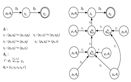
Figure 4: The automata $\mathcal{A}$ (left) and $\mathcal{A}_{post^{*}}$ (right)

Example 4.

Let us illustrate this procedure by an example. Consider the SM-PDS shown in the left half of Fig. 4 and the automaton $\mathcal{A}$ from Fig. 4 that accepts the set $C=\{(\langle p_{0},\gamma_{0}\gamma_{0}\rangle,\theta_{0})\}$ where $(p_{0},\theta_{0})$ is the initial state and $s_{2}$ is the final state. Then the result $\mathcal{A}_{post^{*}}$ of the algorithm is shown in the right half of Fig. 4. The result is derived through the following steps:

1. First, since $(p_{0},\theta_{0})\xrightarrow{\gamma_{0}}_{T^{\prime}}s_{1}$ and $r_{1}\in\theta_{0}$, Rule $(\beta_{3})$ generates a new state $q_{p_{1}\gamma_{1}}^{\theta_{0}}$ and adds the two transitions: $(p_{1},\theta_{0})\xrightarrow{\gamma_{1}}q_{p_{1}\gamma_{1}}^{\theta_{0}}$ and $q_{p_{1}\gamma_{1}}^{\theta_{0}}\xrightarrow{\gamma_{0}}s_{1}$ to $T^{\prime}$.

2. Since $(p_{1},\theta_{0})\xrightarrow{\gamma_{1}}_{T^{\prime}}q_{p_{1}\gamma_{1}}^{\theta_{0}}$ and $r_{2}\in\theta_{0}$, Rule $(\beta_{3})$ generates a new state $q_{p_{2}\gamma_{2}}^{\theta_{0}}$ and adds two transitions : $(p_{2},\theta_{0})\xrightarrow{\gamma_{2}}q_{p_{2}\gamma_{2}}^{\theta_{0}}$ and $q_{p_{2}\gamma_{2}}^{\theta_{0}}\xrightarrow{\gamma_{1}}q_{p_{1}\gamma_{1}}^{\theta_{0}}$ to $T^{\prime}$.

3. Because $(p_{2},\theta_{0})\xrightarrow{\gamma_{2}}_{T^{\prime}}q_{p_{2}\gamma_{2}}^{\theta_{0}}$ and $r_{3}\in\theta_{0}$, Rule $(\beta_{1})$ adds the transition $(p_{3},\theta_{0})\xrightarrow{\gamma_{0}}q_{p_{2}\gamma_{2}}^{\theta_{0}}$ to $T^{\prime}$.

4. Since $(p_{3},\theta_{0})\xrightarrow{\gamma_{0}}_{T^{\prime}}q_{p_{2}\gamma_{2}}^{\theta_{0}}$ and $r^{\prime}\in\theta_{0}$, Rule $(\beta_{4})$ adds the transition $(p_{4},\theta_{1})\xrightarrow{\gamma_{0}}q_{p_{2}\gamma_{2}}^{\theta_{0}}$ to $T^{\prime}$ where $\theta_{1}=(\theta_{0}\setminus\{r_{3}\})\cup\{r_{5}\}=\{r_{1},r_{2},r_{4},r_{5},r^{\prime}\}$.

5. Since $(p_{4},\theta_{1})\xrightarrow{\gamma_{0}}_{T^{\prime}}q_{p_{2}\gamma_{2}}^{\theta_{0}}$ and $r_{4}\in\theta_{1}$, Rule $(\beta_{1})$ adds the transition $(p_{1},\theta_{1})\xrightarrow{\epsilon}q_{p_{2}\gamma_{2}}^{\theta_{0}}$ to $T^{\prime}$.

6. Then, since there is a path $(p_{1},\theta_{1})\xrightarrow{\gamma_{1}}_{T^{\prime}}^{*}q_{p_{1}\gamma_{1}}^{\theta_{0}}$ and $r_{2}\in\theta_{1}$, Rule $(\beta_{3})$ generates new state $q_{p_{2},\gamma_{2}}^{\theta_{1}}$ and adds two transitions $(p_{2},\theta_{1})\xrightarrow{\gamma_{2}}q_{p_{2},\gamma_{2}}^{\theta_{1}}$ and $q_{p_{2},\gamma_{2}}^{\theta_{1}}\xrightarrow{\gamma_{1}}q_{p_{1}\gamma_{1}}^{\theta_{0}}$ to $T^{\prime}$.

7. Since $(p_{2},\theta_{1})\xrightarrow{\gamma_{2}}_{T^{\prime}}q_{p_{2},\gamma_{2}}^{\theta_{1}}$ and $r_{5}\in\theta_{1}$, Rule $(\beta_{2})$ adds the transition $(p_{4},\theta_{1})\xrightarrow{\gamma_{1}}q_{p_{2},\gamma_{2}}^{\theta_{1}}$ to $T^{\prime}$.

8. No unprocessed matches remain. The procedure terminates.

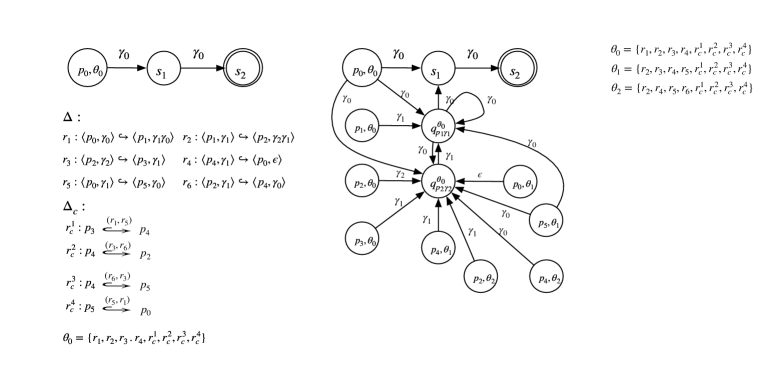
Figure 5: The automata $\mathcal{A}$ (left) and $\mathcal{A}_{post^{*}}$ (right)

Example 5.

Let us illustrate this procedure by another example. Consider the SM-PDS shown in the left half of Fig. 5 where $(p_{0},\theta_{0})$ is the initial state and $s_{2}$ is the final state. The result $\mathcal{A}_{post^{*}}$ of the algorithm is shown in the right half of Fig. 5 obtained as follows:

1. First, since $(p_{0},\theta_{0})\xrightarrow{\gamma_{0}}_{T^{\prime}}s_{1}$ and $r_{1}\in\theta_{0}$, Rule $(\beta_{3})$ generates a new state $q_{p_{1}\gamma_{1}}^{\theta_{0}}$ and adds two transitions: $(p_{1},\theta_{0})\xrightarrow{\gamma_{1}}q_{p_{1}\gamma_{1}}^{\theta_{0}}$ and $q_{p_{1}\gamma_{1}}^{\theta_{0}}\xrightarrow{\gamma_{0}}s_{1}$ to $T^{\prime}$.

2. Since $(p_{1},\theta_{0})\xrightarrow{\gamma_{1}}_{T^{\prime}}q_{p_{1}\gamma_{1}}^{\theta_{0}}$ and $r_{2}\in\theta_{0}$, Rule $(\beta_{3})$ generates a new state $q_{p_{2}\gamma_{2}}^{\theta_{0}}$ and adds two transitions: $(p_{2},\theta_{0})\xrightarrow{\gamma_{2}}q_{p_{2}\gamma_{2}}^{\theta_{0}}$ and $q_{p_{2}\gamma_{2}}^{\theta_{0}}\xrightarrow{\gamma_{1}}q_{p_{1}\gamma_{1}}^{\theta_{0}}$ to $T^{\prime}$.

3. Because $(p_{2},\theta_{0})\xrightarrow{\gamma_{2}}_{T^{\prime}}q_{p_{2}\gamma_{2}}^{\theta_{0}}$ and $r_{3}\in\theta_{0}$, Rule $(\beta_{2})$ adds $(p_{3},\theta_{0})\xrightarrow{\gamma_{1}}q_{p_{2}\gamma_{2}}^{\theta_{0}}$ to $T^{\prime}$.

4. Since $(p_{3},\theta_{0})\xrightarrow{\gamma_{1}}_{T^{\prime}}q_{p_{2}\gamma_{2}}^{\theta_{0}}$ and $r_{c}^{1},r_{1}\in\theta_{0}$, Rule $(\beta_{4})$ adds the transition $(p_{4},\theta_{1})\xrightarrow{\gamma_{1}}q_{p_{2}\gamma_{2}}^{\theta_{0}}$ to $T^{\prime}$ where $\theta_{1}=(\theta_{0}\setminus\{r_{1}\})\cup\{r_{5}\}$.

5. Since $(p_{4},\theta_{1})\xrightarrow{\gamma_{1}}_{T^{\prime}}q_{p_{2}\gamma_{2}}^{\theta_{0}}$ and $r_{4}\in\theta_{1}$, Rule $(\beta_{1})$ adds the transition $(p_{0},\theta_{1})\xrightarrow{\epsilon}q_{p_{2}\gamma_{2}}^{\theta_{0}}$ to $T^{\prime}$. Then there is a path $(p_{0},\theta_{1})\xrightarrow{\gamma_{1}}_{T^{\prime}}^{*}q_{p_{1}\gamma_{1}}^{\theta_{0}}$, since $r_{5}\in\theta_{1}$, Rule $(\beta_{2})$ adds the transition $(p_{5},\theta_{1})\xrightarrow{\gamma_{0}}q_{p_{1}\gamma_{1}}^{\theta_{0}}$ to $T^{\prime}$.

6. Since $(p_{5},\theta_{1})\xrightarrow{\gamma_{0}}_{T^{\prime}}q_{p_{1}\gamma_{1}}^{\theta_{0}}$ and $r_{c}^{4},r_{5}\in\theta_{1}$, Rule $(\beta_{4})$ adds the transition $(p_{0},\theta_{0})\xrightarrow{\gamma_{0}}q_{p_{1}\gamma_{1}}^{\theta_{0}}$ to $T^{\prime}$ where $(\theta_{1}\setminus\{r_{5}\})\cup\{r_{1}\}=\theta_{0}$.

7. Since $(p_{0},\theta_{0})\xrightarrow{\gamma_{0}}_{T^{\prime}}q_{p_{1}\gamma_{1}}^{\theta_{0}}$ and $r_{1}\in\theta_{0}$, Rule $(\beta_{3})$ adds the transitions $(p_{1},\theta_{0})\xrightarrow{\gamma_{1}}q_{p_{1}\gamma_{1}}^{\theta_{0}}$ and $q_{p_{1}\gamma_{1}}^{\theta_{0}}\xrightarrow{\gamma_{0}}q_{p_{1}\gamma_{1}}^{\theta_{0}}$ to $T^{\prime}$.

8. Because $(p_{4},\theta_{1})\xrightarrow{\gamma_{1}}_{T^{\prime}}q_{p_{2}\gamma_{2}}^{\theta_{0}}$ and $r_{c}^{2}\in\theta_{1}$, Rule $(\beta_{4})$ adds the transition $(p_{2},\theta_{2})\xrightarrow{\gamma_{1}}q_{p_{2}\gamma_{2}}^{\theta_{0}}$ to $T^{\prime}$.

9. Since $(p_{2},\theta_{2})\xrightarrow{\gamma_{1}}_{T^{\prime}}q_{p_{2}\gamma_{2}}^{\theta_{0}}$ and $r_{6}\in\theta_{2}$, Rule $(\beta_{2})$ adds the transition $(p_{4},\theta_{2})\xrightarrow{\gamma_{0}}q_{p_{2}\gamma_{2}}^{\theta_{0}}$ to $T^{\prime}$.

10. Since $p_{4},\theta_{2}\xrightarrow{\gamma_{0}}_{T^{\prime}}q_{p_{2}\gamma_{2}}^{\theta_{0}}$ holds and $r_{6},r_{c}^{3}\in\theta_{2}$, Rule $(\beta_{4})$ adds the transition $(p_{5},\theta_{1})\xrightarrow{\gamma_{0}}q_{p_{2}\gamma_{2}}^{\theta_{0}}$ to $T^{\prime}$.

11. Then, since $(p_{5},\theta_{1})\xrightarrow{\gamma_{0}}_{T^{\prime}}q_{p_{2}\gamma_{2}}^{\theta_{0}}$ and $r_{c}^{4}\in\theta_{1}$, Rule $(\beta_{4})$ adds the transition $(p_{0},\theta_{0})\xrightarrow{\gamma_{0}}q_{p_{2}\gamma_{2}}^{\theta_{0}}$ to $T^{\prime}$.

12. Since $r_{1}\in\theta_{0}$ and $(p_{0},\theta_{0})\xrightarrow{\gamma_{0}}_{T^{\prime}}q_{p_{2}\gamma_{2}}^{\theta_{0}}$, Rule ($\beta_{3}$) adds two transitions: $(p_{1},\theta_{0})\xrightarrow{\gamma_{1}}q_{p_{1}\gamma_{1}}^{\theta_{0}}$ and $q_{p_{1}\gamma_{1}}^{\theta_{0}}\xrightarrow{\gamma_{0}}q_{p_{2}\gamma_{2}}^{\theta_{0}}$ to $T^{\prime}$.

13. No more rules can be applied. Thus, the procedure terminates.

VI-A Proof of Theorem 4

Let us now prove Theorem 4. To prove this theorem, we first show the following lemma:

Lemma 3.

For every configuration $(\langle p,w\rangle,\theta_{0})\in L(A)$, if $(\langle p,w\rangle,\theta_{0})\Rightarrow^{*}(\langle p^{\prime},w^{\prime}\rangle,\theta)$ then we have a path $\pi=(p^{\prime},\theta)\xlongrightarrow{w^{\prime}}_{T^{\prime}}q$ for some final state $q$ of $\mathcal{A}_{post^{*}}$.

Proof: 

Let $i$ be the index s.t. $(\langle p,w\rangle,\theta_{0})\stackrel{{\scriptstyle i}}{{\Rightarrow}}(\langle p^{\prime},w^{\prime}\rangle,\theta)$ holds. We proceed by induction on $i$.

Basis. $i=0$. Then $p^{\prime}=p$, $w=w^{\prime}$ and $\theta_{0}=\theta$. Since $(\langle p,w\rangle,\theta_{0})\in L(A)$, we have $(p,\theta_{0})\xlongrightarrow{w}_{T^{\prime}}q$ for some final state $q$ that implies $\pi=(p^{\prime},\theta)\xlongrightarrow{w^{\prime}}_{T^{\prime}}q$ is a path of $\mathcal{A}_{post^{*}}$.

Step. $i>0.$ Then there exists a configuration $(\langle p^{\prime\prime},u\rangle,\theta^{\prime\prime})$ with

$$(\langle p,w\rangle,\theta_{0})\stackrel{{\scriptstyle i-1}}{{\Rightarrow}}(\langle p^{\prime\prime},u\rangle,\theta^{\prime\prime})\Rightarrow(\langle p^{\prime},w^{\prime}\rangle,\theta)$$

By applying the induction hypothesis (induction on $i$), we can get that

$$(p^{\prime\prime},\theta^{\prime\prime})\xlongrightarrow{u}_{T^{\prime}}q\text{ for some }q\in F$$ (1)

Then, let $\gamma\in\Gamma$, $u_{1},w_{1}\in\Gamma^{*}$ be such that $u=\gamma u_{1}$, $w^{\prime}=w_{1}u_{1}$. Let $q_{1}$ be a state of $\mathcal{A}_{post^{*}}$ s.t. we have the following path in $\mathcal{A}_{post^{*}}$:

$$(p^{\prime\prime},\theta^{\prime\prime})\xrightarrow{\gamma}_{T^{\prime}}q_{1}{\mathop{{\hbox{{$\mathrel{\mathop{\hbox to13.00722pt{\rightarrowfill}}\limits^{u_{1}}}$}}}}}_{T^{\prime}}q$$ (2)

There are two cases depending on whether $(\langle p^{\prime\prime},u\rangle,\theta^{\prime\prime})\Rightarrow(\langle p^{\prime},w^{\prime}\rangle,\theta)$ is corresponding to a self-modifying transition (i.e. ($\theta^{\prime\prime}=\theta$)) or not.

1. Case: $\theta^{\prime\prime}=\theta$. Then there exists a transition rule $r:\langle p^{\prime\prime},\gamma\rangle\hookrightarrow\langle p^{\prime},w_{1}\rangle\in\Delta$ s.t. $r\in\theta$. There are three possible cases depending on the length of $w_{1}:$

   1. Case $|w_{1}|=0$ i.e. $w_{1}=\epsilon$, by applying the saturation rule $\beta_{1}$, we can get

      $$(p^{\prime},\theta)\xrightarrow{\epsilon}_{T^{\prime}}q_{1}$$ (3)

      Putting (2) and (3) together, we can have $(p^{\prime},\theta)\xrightarrow{\epsilon}_{T^{\prime}}q_{1}\mathop{{\hbox{{$\mathrel{\mathop{\hbox to13.00722pt{\rightarrowfill}}\limits^{u_{1}}}$}}}}_{T^{\prime}}q$ i.e. $(p^{\prime},\theta)\xrightarrow{w^{\prime}}_{T^{\prime}}q$ for some final state $q$ of $\mathcal{A}_{post^{*}}$.

   2. Case $|w_{1}|=1,$ then let $\gamma^{\prime}\in\Gamma$ s.t. $w_{1}=\gamma^{\prime}$. By applying the saturation rule $\alpha_{2}$, we can get

      $$(p^{\prime},\theta)\xrightarrow{\gamma^{\prime}}_{T^{\prime}}q_{1}$$ (4)

      Putting (2) and (4) together, we can have $(p^{\prime},\theta)\xrightarrow{\gamma^{\prime}}_{T^{\prime}}q_{1}\mathop{{\hbox{{$\mathrel{\mathop{\hbox to13.00722pt{\rightarrowfill}}\limits^{u_{1}}}$}}}}_{T^{\prime}}q$ i.e. $(p^{\prime},\theta)\xrightarrow{w^{\prime}}_{T^{\prime}}q$ for some final state $q$ of $\mathcal{A}_{post^{*}}$.

   3. Case $|w_{1}|=2,$ let $\gamma_{0}^{\prime},\gamma_{1}^{\prime}\in\Gamma$ be such that $w_{1}=\gamma_{0}^{\prime}\gamma_{1}^{\prime}$. By applying the saturation rule $\alpha_{3}$, we can get

      $$(p^{\prime},\theta){\mathop{{\hbox{{$\mathrel{\mathop{\hbox to12.62413pt{\rightarrowfill}}\limits^{\gamma_{0}^{\prime}}}$}}}}}_{T^{\prime}}q^{\theta}_{p^{\prime}\gamma_{0}^{\prime}}{\mathop{{\hbox{{$\mathrel{\mathop{\hbox to12.62413pt{\rightarrowfill}}\limits^{\gamma_{1}^{\prime}}}$}}}}}_{T^{\prime}}q_{1}$$ (5)

      Putting (2) and (5) together, then we have a path $(p^{\prime},\theta)\xrightarrow{\gamma_{0}^{\prime}}_{T^{\prime}}q^{\theta}_{p^{\prime}\gamma_{0}^{\prime}}\xrightarrow{\gamma_{1}^{\prime}}_{T^{\prime}}q_{1}\xrightarrow{u_{1}}_{T^{\prime}}q$ i.e. $(p^{\prime},\theta)\xrightarrow{w^{\prime}}_{T^{\prime}}q$ for some final state $q$ of $\mathcal{A}_{post^{*}}$.

2. Case $\theta^{\prime\prime}\neq\theta$. Then there exists a self-modifying transition rule s.t. $r:p^{\prime\prime}\stackrel{{\scriptstyle(r_{1},r_{2})}}{{\lhook\joinrel\relbar\joinrel\relbar\joinrel\relbar\joinrel\relbar\joinrel\rightarrow}}p^{\prime}\in\Delta_{c}\cap\theta^{\prime\prime}$ and $\gamma=w_{1}$ and $\theta=(\theta^{\prime\prime}\backslash\{r_{1}\})\cup\{r_{2}\}$.

   By applying rule $\beta_{4}$ to (2), we have the following path in the automaton:

   $$(p^{\prime},\theta)\xrightarrow{\gamma}_{T^{\prime}}q_{1}\xrightarrow{u_{1}}_{T^{\prime}}q$$ (5)

   i.e. $(p^{\prime},\theta)\xrightarrow{w^{\prime}}_{T^{\prime}}q$ for some final state $q$ of $\mathcal{A}_{post^{*}}$.

$\;\;\Box$

Lemma 4.

If a path $\pi=(p,\theta)\xrightarrow{w}_{T^{\prime}}q$ is in $\mathcal{A}_{post^{*}}$, then the following holds:

1. if $q$ is a state of $\mathcal{A}$, then $(\langle p^{\prime},w^{\prime}\rangle,\theta_{0})\Rightarrow^{*}(\langle p,w\rangle,\theta)$ for a configuration $(\langle p^{\prime},w^{\prime}\rangle,\theta_{0})$ such that $(p^{\prime},\theta_{0})\xrightarrow{w^{\prime}}_{T}q$ is a path in the initial $\mathcal{P}$-automaton $\mathcal{A}$ ;

2. if $q$ is a new state of the form $q=q_{p_{1}\gamma_{1}}^{\theta_{1}}$, then $(\langle p_{1},\gamma_{1}\rangle,\theta_{1})\Rightarrow^{*}(\langle p,w\rangle,\theta)$.

Proof:  Let $\mathcal{A}_{post^{*}}=({Q^{\prime}},\Gamma,{T^{\prime}},P,F)$ be the $\mathcal{P}$-automaton computed by the saturation procedure. In this proof, we use $\xlongrightarrow[i]{}_{T^{\prime}}$ to denote the transition relation $\rightarrow_{T^{\prime}}$ of $\mathcal{A}_{post^{*}}$ obtained after adding $i$ transitions using the saturation procedure.

Let $i$ be an index such that $(p,\theta)\xlongrightarrow[i]{w}_{T^{\prime}}q$ holds. We prove both parts of the lemma by induction on $i$.

Basis. $i=0$. Only (I) applies. Thus, $p^{\prime}=p$, $\theta_{0}=\theta$ and $w=w^{\prime}$. $(\langle p^{\prime},w^{\prime}\rangle,\theta)\Rightarrow^{*}(\langle p^{\prime},w^{\prime}\rangle,\theta)$ always holds.

Step. $i>1$. Let $t$ be the $i$-th transition added to the automaton. Let $j$ be the number of times that $t$ is used in $(p,\theta)\xlongrightarrow[i]{w}_{T^{\prime}}q$. $\mathcal{A}$ has no transitions leading to initial states, and the algorithm does not add any such transitions; therefore, if $t$ starts in an initial state, $t$ can only be used at the start of the path.

The proof is by induction on $j$. If $j=0$, then we have $(p,\theta)\xrightarrow[i-1]{w}_{T^{\prime}}q$. We apply the induction hypothesis (induction on $i$) then we obtain that there exists a configuration $(\langle p^{\prime},w^{\prime}\rangle,\theta_{0})$ s.t. $(\langle p^{\prime},w^{\prime}\rangle,\theta_{0})\Rightarrow^{*}(\langle p,w\rangle,\theta)$ and $(p^{\prime},\theta_{0})\xrightarrow{w^{\prime}}_{T}q$ is a path of initial $\mathcal{P}$-automaton $\mathcal{A}$. So assume that $j>0$. We distinguish three possible cases:

1. If $t$ was added by the rule $\beta_{1}$, $\beta_{2}$ or $\beta_{3}$, then $t=((p_{1},\theta_{1}),v,q_{1})$, where $v=\epsilon$ or $v=\gamma_{1}$. Then, necessarily, $j=1$ and there exists the following path in the current automaton:

   $$(p,\theta)=(p_{1},\theta_{1})\xlongrightarrow[i]{v}_{T^{\prime}}q_{1}\xlongrightarrow[i-1]{w_{1}}_{T^{\prime}}q$$ (1)

   There are 2 cases depending on whether transition $t$ was added by rule $\beta_{4}$ or not.

   1. Case $t$ was added by rule $\beta_{4}$: there exists a self-modifying transition rule such that $r=p_{2}\stackrel{{\scriptstyle(r_{1},r_{2})}}{{\lhook\joinrel\relbar\joinrel\relbar\joinrel\relbar\joinrel\relbar\joinrel\rightarrow}}p_{1}\in\Delta_{c}$, and there exists the following path in the current automaton:

      $$(p_{2},\theta_{2})\xlongrightarrow[i-1]{v}_{T^{\prime}}q_{1}\xlongrightarrow[i-1]{w_{1}}_{T^{\prime}}q,\theta_{1}=\theta_{2}\backslash\{r_{1}\}\cup\{r_{2}\}$$ (2)

      By induction on $(i)$, we get from (2) that there exists a configuration $(\langle p^{\prime},w^{\prime}\rangle,\theta_{0})$ s.t. $(p^{\prime},\theta_{0})\xrightarrow{w^{\prime}}_{T}q$ is a path in the initial $\mathcal{P}$-automaton $\mathcal{A}$:

      $$(\langle p^{\prime},w^{\prime}\rangle,\theta_{0})\Rightarrow^{*}(\langle p_{2},vw_{1}\rangle,\theta_{2})$$ (3)

      By applying the rule $p_{2}\stackrel{{\scriptstyle(r_{1},r_{2})}}{{\lhook\joinrel\relbar\joinrel\relbar\joinrel\relbar\joinrel\relbar\joinrel\rightarrow}}p_{1}$, we get that

      $$(\langle p_{2},vw_{1}\rangle,\theta_{2})\Rightarrow(\langle p_{1},vw_{1}\rangle,\theta_{1})$$ (4)

      Thus, putting (3) and (4) together, we get that there exists a configuration $(\langle p^{\prime},w^{\prime}\rangle,\theta_{0})$ s.t. $(p^{\prime},\theta_{0})\xrightarrow{w^{\prime}}_{T}q$ is a path in the initial $\mathcal{P}$-automaton $\mathcal{A}$ and:

      $$(\langle p^{\prime},w^{\prime}\rangle,\theta_{0})\Rightarrow^{*}(\langle p_{2},vw_{1}\rangle,\theta_{2})\Rightarrow$$ (5)

      $$(\langle p_{1},w\rangle,\theta_{1})=(\langle p,w\rangle,\theta)$$

   2. Case $t$ is added by $\beta_{1}$ or $\beta_{2}$: then there exists $p_{2}\in P$, $\gamma_{2}\in\Gamma$ such that

      $$r=\langle p_{2},\gamma_{2}\rangle\hookrightarrow\langle p_{1},v\rangle\in\Delta$$ (6)

      and $\mathcal{A}_{post^{*}}$ contains the following path:

      $$(p_{2},\theta_{1})\xlongrightarrow[i-1]{\gamma_{2}}_{T^{\prime}}q_{1}\xlongrightarrow[i-1]{w_{1}}_{T^{\prime}}q$$ (7)

      By induction on $(i)$, We can get from (7) that there exists a configuration $(\langle p^{\prime},w^{\prime}\rangle,\theta_{0})$ s.t. $(p^{\prime},\theta_{0})\xrightarrow{w^{\prime}}_{T}q$ is a path in the initial $\mathcal{P}$-automaton $\mathcal{A}$ and:

      $$(\langle p^{\prime},w^{\prime}\rangle,\theta_{0})\Rightarrow^{*}(\langle p_{2},\gamma_{2}w_{1}\rangle,\theta_{1})$$ (8)

      Thus, putting (6) and (8) together, we have that there exists a configuration $(\langle p^{\prime},w^{\prime}\rangle,\theta_{0})$ s.t. $(p^{\prime},\theta_{0})\xrightarrow{w^{\prime}}_{T}q$ is a path in the initial $\mathcal{P}$-automaton $\mathcal{A}$ and:

      $$(\langle p^{\prime},w^{\prime}\rangle,\theta_{0})\Rightarrow^{*}(\langle p_{2},\gamma_{2}w_{1}\rangle,\theta_{1})\Rightarrow$$ (9)

      $$(\langle p_{1},w\rangle,\theta_{1})=(\langle p,w\rangle,\theta)$$

2. If $t$ is the first transition added by rule $\beta_{3}$ i.e. $t$ is in the form of $((p_{1},\theta^{\prime\prime}),\gamma_{1},q_{p_{1}\gamma_{1}}^{\theta_{1}})$. If this transition is new, then there are no transitions outgoing from $q_{p_{1}\gamma_{1}}^{\theta_{1}}$. So the only path using $t$ is $(p_{1},\theta^{\prime\prime})\xlongrightarrow[i]{\gamma_{1}}_{T^{\prime}}q_{p_{1}\gamma_{1}}^{\theta_{1}}$. For this path, we only need to prove part (II), and $(\langle p_{1},\gamma_{1}\rangle,\theta_{1})\Rightarrow^{*}(\langle p_{1},\gamma_{1}\rangle,\theta_{1})$ holds trivially.

3. Let $t=(q_{p_{1}\gamma_{1}}^{\theta_{1}},\gamma^{\prime\prime},q^{\prime})$ be the second transition added by saturation rule $\beta_{3}$. Then there exist $u$, $v\in\Gamma^{*}$ s.t. $w=u\gamma^{\prime\prime}v$ and the current automaton contains the following path:

   $$(p,\theta)\xlongrightarrow[i-1]{u}_{T^{\prime}}q_{p_{1}\gamma_{1}}^{\theta_{1}}\xlongrightarrow[i]{\gamma^{\prime\prime}}_{T^{\prime}}q^{\prime}\xlongrightarrow[i]{v}_{T^{\prime}}q$$ (10)

   Because $t$ was added via the saturation rule, then there exist $p_{2}\in P$, $\gamma_{2}\in\Gamma$ and a rule of the form

   $$\langle p_{2},\gamma_{2}\rangle\hookrightarrow\langle p_{1},\gamma_{1}\gamma^{\prime\prime}\rangle\in\Delta\cap\theta_{1}$$ (11)

   and $\mathcal{A}_{post^{*}}$ contains the following path:

   $$(p_{2},\theta_{1})\xlongrightarrow[i-1]{\gamma_{2}}_{T^{\prime}}q^{\prime}\xlongrightarrow[i]{v}_{T^{\prime}}q$$ (12)

   We apply the induction hypothesis on $i$ and obtain that

   $$(\langle p_{1},\gamma_{1}\rangle,\theta_{1})\Rightarrow^{*}(\langle p,u\rangle,\theta)$$ (13)

   We apply the induction hypothesis on $i$ to obtain that there exists a configuration $(\langle p^{\prime},w^{\prime}\rangle,\theta_{0})$ s.t. $(p^{\prime},\theta_{0})\xrightarrow{w^{\prime}}_{T}q$ is a path in the initial $\mathcal{P}$-automaton $\mathcal{A}$ and:

   $$(\langle p^{\prime},w^{\prime}\rangle,\theta_{0})\Rightarrow^{*}(\langle p_{2},\gamma_{2}v\rangle,\theta_{1})$$ (14)

   Thus, putting (11) (13) and (14) together, we have that there exists a configuration $(\langle p^{\prime},w^{\prime}\rangle,\theta_{0})$ s.t. $(p^{\prime},\theta_{0})\xrightarrow{w^{\prime}}_{T}q$ is a path in the initial $\mathcal{P}$-automaton $\mathcal{A}$ and:

   $$(\langle p^{\prime},w^{\prime}\rangle,\theta_{0})\Rightarrow^{*}(\langle p_{2},\gamma_{2}v\rangle,\theta_{1})\Rightarrow$$ (15)

   $$(\langle p_{1},\gamma_{1}\gamma^{\prime\prime}v\rangle,\theta_{1})\Rightarrow^{*}(\langle p,u\gamma^{\prime\prime}v\rangle,\theta)=(\langle p,w\rangle,\theta)$$

$\;\;\Box$

Then we continue to prove Theorem 4:

Proof:  Let $(\langle p^{\prime},w^{\prime}\rangle,\theta)$ be a configuration of $post^{*}(L(\mathcal{A}))$. Then there exists a configuration $(\langle p,w\rangle,\theta_{0})$ such that there exists a path $(p,\theta_{0})\xrightarrow{w}_{T}q$ in the initial automaton $\mathcal{A}$ and $(\langle p,w\rangle,\theta_{0})\Rightarrow^{*}(\langle p^{\prime},w^{\prime}\rangle,\theta)$. By Lemma 3, we can have $(p^{\prime},\theta)\xrightarrow{w^{\prime}}_{T^{\prime}}q$ for $q$ is a final state of $\mathcal{A}_{post^{*}}$. So $(\langle p^{\prime},w^{\prime}\rangle,\theta)$ is recognized by $\mathcal{A}_{post^{*}}$.

Conversely, let $(\langle p^{\prime},w^{\prime}\rangle,\theta)$ be a configuration recognized by $\mathcal{A}_{post^{*}}$. Then there exists a path $(p^{\prime},\theta)\xrightarrow{w^{\prime}}_{T^{\prime}}q$ in $\mathcal{A}_{post^{*}}$ for some final state $q$. By Lemma 4, since $q$ is a final state, we have $(\langle p,w\rangle,\theta_{0})\Rightarrow_{\mathcal{P}}^{*}(\langle p^{\prime},w^{\prime}\rangle,\theta)$ s.t. there exists a configuration $(\langle p,w\rangle,\theta_{0})$ s.t. $(p,\theta_{0})\xrightarrow{w}_{T^{\prime}}q$ is a path in the initial automaton $\mathcal{A}$ i.e. $(\langle p,w\rangle,\theta_{0})\in L(A)$. Therefore, $(\langle p^{\prime},w^{\prime}\rangle,\theta)\in post^{*}(L(A))$

$\;\;\Box$

VII Experiments

VII-A Our algorithms vs. standard $pre^{*}$ and $post^{*}$ algorithms of PDSs

$|\Delta|+|\Delta_{c}|$	SM-PDS	PDS	Result1	Total1	Symbolic PDS	Result2	Total2
$10+3$	0.08s & 2MB	0.15s & 3MB	0.00s	0.15s	0.10s & 2MB	0.00s	0.10s
$13+3$	0.10s & 2MB	0.15s & 3MB	0.00s	0.15s	0.10s & 2MB	0.00s	0.10s
$13+3$	0.12s & 2MB	0.15s & 3MB	0.00s	0.15s	0.10s & 2MB	0.00s	0.10s
$43+7$	0.24s &3MB	3.44s &4MB	0.02s	3.46s	4.80s &5MB	0.01s	4.81s
$110+10$	0.38s &7MB	5.15s &6MB	0.01s	5.16s	2.71s &8MB	0.00s	2.71s
$120+10$	0.42s &11MB	5.20s &15MB	0.01s	5.21s	2.79s &10MB	0.01s	2.80s
$255+8$	0.65s & 15MB	295.41s & 86MB	0.05s	295.46s	21.41s & 76MB	0.02s	21.43s
$1009+10$	1.49s &97MB	11504.2s & 117MB	2.46s	11506.66s	14.10s &471MB	1.74s	15.84s
$1899+7$	2.98s & 210MB	6538s & 171MB	4.09s	6542.09s	124.10s & 558MB	2.71s	173.71s
$2059+8$	3.82s &423MB	19525.1s &113MB	4.19s	19529.29s	20.70s &713MB	error	-
$2099+8$	4.05s & 32MB	19031s & 192MB	4.19s	19035.19s	124.12s & 757MB	error	-
$2099+9$	7.08s & 252MB	29742s & 198MB	4.28s	29746.28s	128.12s & 760MB	error	-
$3060+9$	11.36s & 282MB	29993.05s & 241MB	18.72s	30011.77s	261.07s & 610MB	error	-
$3160+9$	11.99s & 285MB	29252.05s & 257MB	26.15s	29278.2s	162.55s & 611MB	error	-
$4058+7$	18.06s & 332MB	81408.51s &307MB	92.68s	81501.19s	802.07s &1013MB	error	-
$4058+8$	19.42s & 397MB	82812.51s &399MB	91.91s	82904.42s	899.07s & 1020MB	error	-
$4158+8$	21.68s &491MB	83112.51s &401MB	97.68s	83210.19	899.19s &1021MB	error	-
$5050+8$	23.26s &499MB	93912.51s &298MB	118.12	94030.63s	205.12s &375MB	error	-

TABLE I: Our direct $pre^{*}$ algorithm vs. standard $pre^{*}$ algorithms of PDSs

We implemented our algorithms in a tool. To compare the performance of our algorithms against the approach that consists in translating the SM-PDS into an equivalent PDS or symbolic PDS and then apply the standard $post^{*}$ and $pre^{*}$ algorithms for PDSs and symbolic PDSs [EHRS00, Sch02], we first applied our tool on randomly generated SM-PDSs of various sizes. The results of the comparision using the $pre^{*}$ (resp. $post^{*}$) algorithms are reported in Table 1 (resp. Table 2).

$|\Delta|+|\Delta_{c}|$	SM-PDS	PDS	Result1	Total1	Symbolic PDS	Result2	Total2
$10+3$	0.12s & 2MB	0.15s & 3MB	0.00s	0.15s	0.10s &2MB	0.00s	0.10s
$13+3$	0.12s & 2MB	0.15s &3MB	0.00s	0.15s	0.10s &2MB	0.00s	0.10s
$43+7$	0.28s & 2MB	3.44s & 4MB	0.04s	3.48s	4.80s & 5MB	0.02s	4.82s
$110+10$	0.36s & 8MB	5.15s &6MB	0.01s	5.16s	2.71s &8MB	0.00s	2.71s
$120+10$	0.39s & 13MB	5.20s &15MB	0.01s	5.21s	2.79s & 10MB	0.01s	2.80s
$255+8$	0.44s & 15MB	295.41s & 86MB	0.05s	295.46s	21.41s & 76MB	0.02s	21.43s
$1009+10$	1.48s & 97MB	11504.2s & 117MB	2.56s	11506.76s	14.10s & 471MB	1.75s	15.85s
$1899+7$	3.47s & 212MB	6538s & 171MB	3.89s	6541.89s	124.10s & 558MB	2.71s	126.81s
$2059+8$	4.03s &323MB	19525.1s & 113MB	3.99s	19528.99s	20.70s &713MB	error	-
$2099+8$	4.15s &332MB	19031s &192MB	3.99s	19034.99s	124.12s & 757MB	error	-
$2099+9$	4.95s & 352MB	29742s & 198MB	4.18s	29746.18s	128.12s & 760MB	error	-
$3060+9$	5.71s & 388MB	29993.05s & 241MB	18.12s	30011.17s	261.07s &610MB	error	-
$3160+9$	5.79s & 415MB	29252.05s & 257MB	26.10s	29278.15s	162.55s & 611MB	error	-
$4058+7$	7.56s & 364MB	81408.51s & 307MB	91.68s	81500.19s	802.07s & 1013MB	error	-
$4058+8$	9.76s & 387MB	82812.51s & 399MB	91.71s	82904.22s	899.07s & 1020MB	error	-
$4158+8$	11.85s & 487MB	83112.51s & 401MB	97.28s	83209.79s	899.19s & 1021MB	error	-
$5050+8$	13.04s & 498MB	93912.51s &498MB	112.53s	94025.04s	205.12s & 375MB	error	-

TABLE II: Our direct $post^{*}$ algorithm vs. standard $post^{*}$ algorithms of PDSs

In Table I, Column $|\Delta|+|\Delta_{c}|$ is the number of transitions of the SM-PDS (changing and non changing rules). Column SM-PDS gives the cost it takes to apply our direct algorithm to compute the $pre^{*}$ for the given SM-PDS. Column PDS shows the cost it takes to get the equivalent PDS from the SM-PDS. Column Symbolic PDS reports the cost it takes to get the equivalent Symbolic PDS from the SM-PDS. Column Result1 reports the cost it takes to get the $pre^{*}$ analysis of Moped [Sch02] for the PDS we got. Column Total1 is the total cost it takes to translate the SM-PDS into a PDS and then apply the standard $pre^{*}$ algorithm of Moped (Total1=PDS+Result1). Column Result2 reports the cost it takes to get the $pre^{*}$ analysis of Moped for the symbolic PDS we got. Column Total2 is the total cost it takes to translate the SM-PDS into a symbolic PDS and then apply the standard $pre^{*}$ algorithm of Moped (Total2=Symbolic PDS+Result2). ”error” in the table means failure of Moped, because the size of the relations involved in the symbolic transitions is huge. Hence, we mark $-$ for the total execution time. You can see that our direct algorithm (Column SM-PDS) is much more efficient.

Table II shows the performance of our $post^{*}$ algorithm. The meaning of the columns are exactly the same as for the $pre^{*}$ case, but using the $post^{*}$ algorithms instead. You can see from this table that applying our direct $post^{*}$ algorithm on the SM-PDS is much better than translating the SM-PDS to an equivalent PDS or symbolic PDS, and then applying the standard $post^{*}$ algorithms of Moped. Going through PDSs or symbolic PDSs is less efficient and leads to memory out in several cases.

VII-B Malware Detection

Self-modifying code is widely used as an obfuscation technique for malware writers. Thus, we applied our tool for malware detection.

Example	SM-PDS	PDS
Email-Worm.Win32.Klez.b	Y	N
Backdoor.Win32.Allaple.b	Y	N
Email-Worm.Win32.Avron.a	Y	N
Email-Worm.Win32.Anar.a	Y	N
Email-Worm.Win32.Anar.b	Y	N
Email-Worm.Win32.Bagle.a	Y	N
Email-Worm.Win32.Bagle.am	Y	N
Email-Worm.Win32.Bagle.ao	Y	N
Email-Worm.Win32.Bagle.ap	Y	N
Email-Worm.Win32.Ardurk.d	Y	N
Email-Worm.Win32.Atak.k	Y	N
Email-Worm.Win32.Atak.g	Y	N
Email-Worm.Win32.Hanged	Y	N

TABLE III: Malware Detection

We consider self-modifying versions of 13 well known malwares. In these versions, the malicious behaviors are unreachable if one does not take into account that the self-modifying piece of code will change the malware code: if the code does not change, the part that contains the malicious behavior cannot be reached; after executing the self-modifying code, the control point will jump to the part containing the malicious behavior.

We model such malwares in two ways: (1) first, we take into account the self-modifying piece of code and use SM-PDSs to represent these programs as discussed in Section III-B, (2) second, we don’t take into account that this part of the code is self-modifying and we treat it as all the other instructions of the program. In this case, we model these programs by a standard PDS following the translation of [ST12].

The results are reported in Table 3, Column Example reports the name of the worm. Column SM-PDS shows the result obtained by applying our method to check the reachability of the entry point of the malicious block. Column PDS gives the result if we apply the traditional PDS translation of programs (without taking into account the semantics of self modifying code) method to check the reachability of the entry point of the malicious block. $Y$ stands for yes (the program is malicious) and $N$ stands for no (the program is benign). As it can be seen, our techniques that go through SM-PDS to model self modifying code is able to conclude that the entry point of the malicious block is reachable, whereas the standard PDS translation from programs fails to reach this conclusion.

References

- [AMDB06] Bertrand Anckaert, Matias Madou, and Koen De Bosschere. A model for self-modifying code. In IH, pages 232–248, 2006.
- [BDD+01] Jean Bergeron, Mourad Debbabi, Jules Desharnais, Mourad M Erhioui, Yvan Lavoie, Nadia Tawbi, et al. Static detection of malicious code in executable programs. Int. J. of Req. Eng, 2001(184-189):79, 2001.
- [BEM97] A. Bouajjani, J. Esparza, and O. Maler. Reachability Analysis of Pushdown Automata: Application to Model Checking. In CONCUR, pages 135–150, 1997.
- [BLP16] Sandrine Blazy, Vincent Laporte, and David Pichardie. Verified abstract interpretation techniques for disassembling low-level self-modifying code. Journal of Automated Reasoning, 56(3):283–308, 2016.
- [BMRP09] Guillaume Bonfante, Jean-Yves Marion, and Daniel Reynaud-Plantey. A computability perspective on self-modifying programs. In SEFM, pages 231–239, 2009.
- [BRK+05] Gogul Balakrishnan, Thomas W. Reps, Nicholas Kidd, Akash Lal, Junghee Lim, David Melski, Radu Gruian, Suan Hsi Yong, Chi-Hua Chen, and Tim Teitelbaum. Model checking x86 executables with codesurfer/x86 and WPDS++. In CAV, pages 158–163, 2005.
- [CDKT09] Kevin Coogan, Saumya Debray, Tasneem Kaochar, and Gregg Townsend. Automatic static unpacking of malware binaries. In WCRE, pages 167–176, 2009.
- [CJS+05] Mihai Christodorescu, Somesh Jha, Sanjit A Seshia, Dawn Song, and Randal E Bryant. Semantics-aware malware detection. In SP, pages 32–46, 2005.
- [CSV07] Hongxu Cai, Zhong Shao, and Alexander Vaynberg. Certified self-modifying code. ACM SIGPLAN Notices, 42(6):66–77, 2007.
- [CT08] Saumya K Debray Kevin P Coogan and Gregg M Townsend. On the semantics of self-unpacking malware code. Technical report, Citeseer, 2008.
- [EHRS00] Javier Esparza, David Hansel, Peter Rossmanith, and Stefan Schwoon. Efficient algorithms for model checking pushdown systems. In CAV, pages 232–247, 2000.
- [Kar] Karl. Automated unpacking: A behaviour based approach. https://github.com/malwaremusings/unpacker.
- [Kin08] Veith H. Kinder.J. Jakstab: A static analysis platform for binaries. In CAV, pages 423–427. Springer, 2008.
- [KKSV05] Johannes Kinder, Stefan Katzenbeisser, Christian Schallhart, and Helmut Veith. Detecting malicious code by model checking. In DIMVA, pages 174–187, 2005.
- [KPY07] Min Gyung Kang, Pongsin Poosankam, and Heng Yin. Renovo: A hidden code extractor for packed executables. In WORM, pages 46–53. ACM, 2007.
- [RHD+06] Paul Royal, Mitch Halpin, David Dagon, Robert Edmonds, and Wenke Lee. Polyunpack: Automating the hidden-code extraction of unpack-executing malware. In ACSAC, pages 289–300, 2006.
- [RM10] Kevin A Roundy and Barton P Miller. Hybrid analysis and control of malware. In International Workshop on Recent Advances in Intrusion Detection, pages 317–338. Springer, 2010.
- [Sch02] Stefan Schwoon. Model-checking pushdown systems. PhD thesis, Technische Universität München, Universitätsbibliothek, 2002.
- [SL03] Prabhat K Singh and Arun Lakhotia. Static verification of worm and virus behavior in binary executables using model checking. In IAW, pages 298–300, 2003.
- [ST12] Fu Song and Tayssir Touili. Efficient malware detection using model-checking. In FM, pages 418–433, 2012.
- [ST13] Fu Song and Tayssir Touili. Ltl model-checking for malware detection. In TACAS, pages 416–431. Springer, 2013.
- [Tea] EnSilo Research Team. Self-modifying code unpacking tool using dynamorio. https://github.com/BreakingMalware/Selfie.
- [TY17] Tayssir Touili and Xin Ye. Reachability analysis of self modifying code. In 2017 22nd International Conference on Engineering of Complex Computer Systems (ICECCS), pages 120–127. IEEE, 2017.