A finite electric-field approach to evaluate the vertex correction for the screened Coulomb interaction in the quasiparticle self-consistent GW method

Abstract

We apply the quasiparticle self-consistent GW method (QSGW) to slab models of ionic materials, LiF, KF, NaCl, MgO, and CaO, under electric field. Then we obtain the optical dielectric constants $\epsilon_{\infty}({\rm Slab})$ from the differences of the slopes of the electrostatic potential in the bulk and vacuum regions. Calculated $\epsilon_{\infty}({\rm Slab})$ show very good agreements with experiments. For example, we have $\epsilon_{\infty}({\rm Slab})$=2.91 for MgO, in agreement with the experimental value $\epsilon_{\infty}(\rm Experiment)$=2.96. This is in contrast to $\epsilon_{\infty}(\rm RPA)$=2.37, which is calculated in the random-phase approximation for the bulk MgO in QSGW. After we explain the difference between the quasiparticle-based perturbation theory and the Green’s function based perturbation theory, we interpret the large difference $\epsilon_{\infty}({\rm Slab})-\epsilon_{\infty}({\rm RPA})=2.91-2.37$ as the contribution from the vertex correction of the proper polarization which determines the screened Coulomb interaction $W$. Our result encourages the theoretical development of self-consistent $G_{0}W$ approximation along the line of QSGW self-consistency, as was performed by Shishkin, Marsman and Kresse [Phys. Rev. Lett. 99, 246403(2007)].

I introduction

The quasiparticle self-consistent GW (QSGW) is one of the most reliable method to determine the one-particle effective Hamiltonian which describes the independent-particle picture, or the quasiparticle (QP) picture, for treating electric excitations of materials Faleev et al. (2004); van Schilfgaarde et al. (2006); Kotani et al. (2007). Other competitive methods such as HSE Heyd et al. (2006) and Tran-Blaha-09 functional Tran and Blaha (2009) may work well in many systems, although we may need to use material-dependent parameters He and Franchini (2012). In contrast, QSGW is virtually parameter free and gives reliable descriptions for a wide range of materials, not only metals and semiconductors, but also transition-metal oxides, type-II superlattice, and $4f$ systems Bruneval and Gatti (2014); Deguchi et al. (2016); Okumura et al. (2019); Lee et al. (2020). Since heterogeneous mixtures of materials are used in current technologies, QSGW is worth to be developed more as a tool to treat electronic structures of such materials, where methods including such material-dependent parameters are hardly applicable.

However, QSGW as it is has a shortcoming that it gives a systematic overestimation of the exchange effects. This results in a little larger band gaps in QSGW for materials. In fact, Faleev, van Schilfgaarge, and Kotani Faleev et al. (2004); van Schilfgaarde et al. (2006); Kotani et al. (2007) made a suggestion that the overestimation is removed if we perform improved QSGW calculations taking into account the enhancement of the screening effect due to the electron-hole correlation in the evaluation of the screened Coulomb interaction $W$. This is based on the theoretical consideration combined with the observation that the calculated optical dielectric constant $\epsilon_{\infty}$ in the random-phase approximation (RPA) in QSGW gives $\sim 20$ percent smaller $\epsilon_{\infty}$ than experiments for kinds of materials Kotani et al. (2007); Bhandari et al. (2018).

Such an improved calculation was performed by Shishkin, Marsman and Kresse, where they include the enhancement of the screening effect Shishkin et al. (2007). The enhancement is via the vertex correction for the proper polarization $P$, which determines $W=v/(1-vP)$, where $v$ denoted the Coulomb interaction. They approximately include the lowest-order vertex correction due to the electron-hole correlation; see Eq.(15) around in Ref.Bruneval et al., 2005. Their results are theoretically quite satisfactory in the sense that both band gaps and $\epsilon_{\infty}$, which are calculated simultaneously and self-consistently without parameters as in HSE, are in agreement with experiments. For example, calculated values $\epsilon_{\infty}=2.96$ and band gap $E_{\rm G}=8.12$eV for MgO are in agreement with the experiments, 2.95, and 7.83 eV, respectively. See sc$GW$(e-h) in Table I in Ref.Shishkin et al., 2007. Furthermore, based on these theoretical analyses, we can introduce QSGW80 to avoid the very expensive computational costs of the method by Shishkin et al.. QSGW80 is just a simple hybridization, 80 % QSGW+ 20 % GGA to include such enhancement of the screening effectively. The hybridization is very different from the hybridization in HSE, where the mixing ratio $\alpha$ between GGA and the Hartree-Fock strongly affects to final results. QSGW80 works well to describe experimental band gaps Chantis et al. (2006). The performance of QSGW80 is systematically examined in Ref.Deguchi et al., 2016 by Deguchi et al., where we see both the calculated band gaps and effective masses are in good agreements with experiments. QSGW80 is successfully used for practical applications, for example, to the type-II superlattice of InAs/GaSb Otsuka et al. (2017); Sawamura et al. (2017).

In this paper, we evaluate $\epsilon_{\infty}$ not in bulk calculations with such approximations used in Ref.Shishkin et al., 2007, but by slab models with finite electric bias voltage. We treat five ionic materials, LiF, KF, NaCl, MgO and CaO. We put a slab in the middle of vacuum region in a supercell. The electric field is applied by the effective screening medium (ESM) method given by Otani and Sugino Otani and Sugino (2006). We obtain $\epsilon_{\infty}$ from the ratio of slopes of the electrostatic fields at slab region and at vacuum region. Our approach is based on the self-consistent method, thus we do not need to utilize approximations as was used in Ref.Shishkin et al., 2007. Since we explicitly treat the response to the bias, our method includes higher-order effects in a self-consistent manner.

Our findings are that the calculated $\epsilon_{\infty}$ in QSGW for the slab models are very close to experimental values. This is in contrast to the fact that $\epsilon_{\infty}$ in RPA of QSGW are generally $\sim$ 20 percent smaller than experimental values. This indicates that the vertex correction at the level of derivative of the QSGW self-energy should make $W$ be in agreements with experiments. Our results is consistent with Table II in Ref.Shishkin et al., 2007.

We can interpret the enhancement of screening, represented by the enlargement of $\epsilon_{\infty}$, as the size of the vertex correction for the proper polarization $P$. Note that the vertex correction we evaluate is not what is defined in the Hedin’s equation Hedin and Lundqvist (1969). In the equation, we see $P=-iGG\Gamma$, that is, the vertex function $\Gamma$ is for the correction to $P=-iGG$, where $G$ denotes the Green’s function. Instead, we rather evaluate $\Gamma$ for $P=-iG_{0}G_{0}\Gamma$, where $G_{0}$ is the bare Green’s function. To clarify the above theoretical point on $\Gamma$, we give an extensive discussion in Sec.II. We explain role of $\Gamma$ in the two kinds of perturbation theories. In Sec.III, we explain QSGW+ESM, an implementation of QSGW combined with ESM. The QSGW+ESM for slab models should be very useful not only for our purpose here, but also for others where usual GGA+ESM have difficulties. In Sec.IV, we show our results of $\epsilon_{\infty}$. Then they are interpreted as the vertex correction. In Sec. IV.2, we give a rationale of QSGW80, followed by a summary.

II QP-based perturbation vs. $G$-based perturbation

To make our motivation in this paper clarified, we have to clarify the difference between the quasiparticle-based perturbation (QbP) and the Green’s function-based perturbation (GbP). QbP is based on the Landau-Silin’s QP theory, while GbP is on the Hedin’s one. To illustrate the difference between QbP and GbP, we give a narrow-band model as follows. The model represent situations where we have good QP picture (= independent-particle picture).

In advance, remind that we mainly have two kinds of excitations in the paramagnetic electronic systems. That is, the multi-particle excitations, and the collective excitation such as plasmons. The former is described by QPs interacting each other. Note that plasmons is located at high energy because of the long-range Coulomb interaction Pines and Nozieres (1966). These excitations can be hybridized. For example, we know pseudo plasmon in Silver, where one-particle excitations of $3d$ electrons are hybridized with plasmons.

II.1 narrow-band model to explain the QP-based perturbation

The QPs based on the Landau-Silin’s Fermi liquid theory is originally for metals Pines and Nozieres (1966). However, the idea of QPs are rather easily applicable to insulators. We can consider QbP based on the QPs. To illustrate this, let us consider a narrow-band model, a paramagnetic case given by a Hamiltonian $H$, which has an one-body term represented by finite numbers of Wannier functions in the primitive cell, and the Coulomb-like interaction $\frac{e^{2}}{\epsilon^{\prime}|{\bf r}-{\bf r}^{\prime}|}$, where $\epsilon^{\prime}$ is a constant. We consider a case that it gives the QPs shown in Fig.1 given by the one-particle Hamiltonian $H_{0}$.

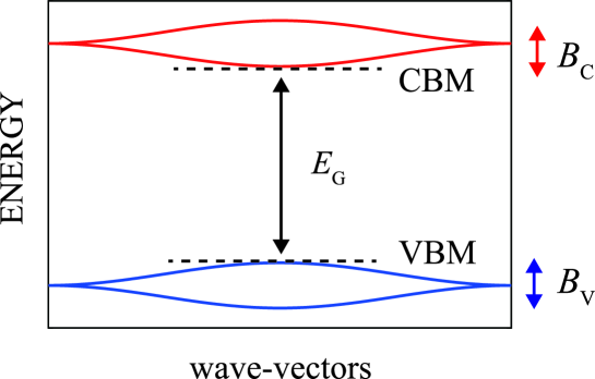
Figure 1: Band structure of a narrow-band model to illustrate the quasiparticle based perturbation. CBM and VBM are the acronyms of conduction-band minimum and valence-band maximum. The width of bands $B_{\rm C}$ and $B_{\rm V}$ are smaller than the band gap $E_{\rm G}$. As in the text, we expect well-defined QPs in this model.

Based on the perturbation, we expect that the lifetimes of all the electrons are infinite because the band gap $E_{\rm G}$ is large enough to forbid all the electrons decaying into lower energy electrons accompanying electron-hole pairs, holes as well. In other words, all bands are within the threshold of impact ionization Kotani and van Schilfgaarde (2010a). Thus QPs described by $G_{0}=1/(\omega-H_{0})$ should give well-defined one-particle excitations of the narrow-band model.

This conclusion should be essentially kept even when we fully turn on the interaction as long as the following conditions are well satisfied. First, excitons, binding states of electron-hole pairs, should be only slightly at lower energies than $E_{\rm G}$. Second, plasmons should be located at high enough energies so that the plasmon are hardly hybridized with the one-particle excitations. Under these assumptions, we have well-defined QPs. We can consider a path of adiabatic connection with keeping the well-defined QPs given by $H_{0}$ since the QP spectrum is clearly separated from the other excitations. It can be written as $H_{\lambda}=H_{0}+(H_{\lambda}-H_{0})$ for $\lambda$ is from zero to unity, where $H=H_{\lambda=1}$. Note that $(H_{\lambda}-H_{0})$ need to contain $\lambda$-dependent one-body term.

In this narrow-band model, QbP should be suitable; QPs are interacting each other by $(H_{\lambda=1}-H_{0})$. As for the proper polarization function, we can take all the non-interacting two-body QP excitations correctly by $P_{0}=-iG_{0}G_{0}$. Based of this QbP, $G_{0}W_{0}$ approximation, $\Sigma=iG_{0}W_{0}$ where $W_{0}=v/(1-vP_{0})$, is physically justified. That is, it describes how the motion of QPs in $G_{0}$ is perturbed by the dynamical self-interaction given by $W_{0}$ in RPA. Most of all first-principles calculations in literatures are implicitly based on this QbP, while some latest literatures Kutepov (2016, 2017) are based on GbP explained in Sec.II.3. QSGW is a method to determine $H_{0}$ self-consistently in QbP.

II.2 vertex function $\Gamma_{\rm QbP}$ in the QP-based perturbation

To improve $G_{0}W_{0}$, we may include electron-hole correlation. The corrections replace $P_{0}=-iG_{0}G_{0}$ with $P$ where we include the correlation via the Bethe-Salpeter equation (ladder diagrams). That is, we include two-body spectrum in the proper polarization accurately. This lets us to use $W=1/(1-vP)$ instead of $W_{0}$, resulting the $G_{0}W$ approximation as $\Sigma=iG_{0}W$. In this paper, we concentrate on the $G_{0}W$ approximation as in the case of sc$GW$(e-h) in Ref.Shishkin et al., 2007. In QbP, we thus define the vertex function $\Gamma_{\rm QbP}$ for $W$ as $P=-iG_{0}G_{0}\Gamma_{\rm QbP}$. Roughly speaking, $P=P_{0}\Gamma_{\rm QbP}$. We give the numerical evaluation for this $\Gamma_{\rm QbP}$ via the evaluation of $\epsilon_{\infty}$ as shown in Sec.IV.1.

To go beyond $\Sigma=iG_{0}W$ approximation here, we need to take into account three-particle intermediate states. However, it is not theoretically straightforward because of a double counting problem that $\Sigma=iG_{0}W$ already partially takes into account such states. We will need to construct theories of three-particle problem without double counting along the line of first-principles calculations. We do not treat this problem in this paper.

II.3 $G$-based perturbation and vertex function $\Gamma_{\rm GbP}$

Let us consider how we can apply GbP to the narrow-band model. In contrast to $G_{0}$ in QbP, the one-body Green function $G$ has complex meanings. We have imaginary part of $G$ at high energies, representing QPs hybridized with plasmons (plasmarons). Because of sum rule for ${\rm Im}[G]$, the QP parts are suppressed by $Z$-factor. Thus there is a problem that $P=-iGG$ do not contain the two-body non-interacting excitations with the correct weight, in contrast to the case $P_{0}=-iG_{0}G_{0}$.

In principle, this problem is corrected by including the vertex function $\Gamma_{\rm GbP}$ in the Hedin’s equation to determine the one-particle Green’s function $G(1,2)$ Hedin and Lundqvist (1969). Because Hedin’s equation is theoretically rigorous, we expect $-iGG\Gamma_{\rm GbP}\approx P_{0}=-iG_{0}G_{0}$ in the model, under the discussion of Sec.II.1 that $P_{0}$ gives good approximation for the model. That is, contributions related to the collective excitations and renormalization factors $Z$ in $-iGG$ should be virtually taken away by the factor $\Gamma_{\rm GbP}$. However, such numerical calculations should be computationally very demanding Bechstedt et al. (1997). Similar discussion of $Z$-factor cancellation is also seen when we multiply $G_{0}$ to $W$. That is, we should have $G_{0}W\approx GW\Gamma_{\rm GbP}$ since QbP correctly treats the model. Our analysis here is consistent with Takada’s analysis based on the Ward identity Takada (2016).

QbP should be generally superior to GbP even in real materials. In contrast to GbP, QbP is quite simple and physically convincing. We should not be confused with the similarity of QbP and GbP. In this paper, we evaluate $\Gamma_{\rm QbP}$. In the following, we calculate the enhancement of the screening effect. Then we evaluate the size of the ratio $P/P_{0}$ from the comparison between calculated $\epsilon_{\infty}$ in RPA and $\epsilon_{\infty}$ in the slab models. This ratio gives the size of $\Gamma_{\rm QbP}$.

III QSGW combined with Effective screening medium method

To calculate $\epsilon_{\infty}$, we put a slab in the middle of vacuum region in a supercell. $\epsilon_{\infty}$ is calculated from the difference of slopes in the vacuum region and in the slab region under small bias voltage. The supercell we use are detailed at the beginning of Sec.IV. In such calculations, we can obtain $\epsilon_{\infty}$ beyond the bulk calculation in RPA as we explain in the next paragraph. That is, we can obtain $\epsilon_{\infty}$ including the effect of the vertex correction.

To explain how the effect is included, let us consider slab calculations in the case of GGA at first. We first perform self-consistent calculation under zero bias. Then we perform self-consistent calculation under the finite bias (theoretically, it should be infinitesimally small). Then we have the difference of the electron density $\delta n({\bf r})$ between the two calculations. Simultaneously, we have a corresponding response of the one-particle potential given as $\delta V({\bf r})=\int d^{3}r^{\prime}v({\bf r}-{\bf r}^{\prime})\delta n({\bf r}^{\prime})+\frac{\partial V^{\rm GGA}_{\rm xc}}{\partial n({\bf r})}\delta n({\bf r})$. The last term is the difference in the exchange-correlation (xc) potential caused by $\delta n({\bf r})$ self-consistently. That is, the derivative $\frac{\delta V({\bf r})}{\delta n({\bf r}^{\prime})}$ contains the contribution of the xc kernel $f_{\rm xc}=\frac{\partial V^{\rm GGA}_{\rm xc}}{\partial n({\bf r})}$. Under the bias, we can obtain $\epsilon_{\infty}$, from the ratio of slopes of the electrostatic potential in the vacuum region and in the slab region. It should contain the contribution from $f_{\rm xc}$, which is identified as the vertex correction in GGA.

This is essentially the same in QSGW. Recall that the self-energy in QSGW denoted as $V^{\rm QSGW}_{\rm xc}({\bf r},{\bf r}^{\prime})$ is a static non-local potential, replacing $V^{\rm GGA}_{\rm xc}$. The derivative of the one-particle potential is given as $\delta V({\bf r},{\bf r}^{\prime})=\int d^{3}r^{\prime\prime}v({\bf r}-{\bf r}^{\prime\prime})\delta n({\bf r}^{\prime\prime})+\delta V^{\rm QSGW}_{\rm xc}({\bf r},{\bf r}^{\prime})$, where the last term play a role of $\frac{\partial V^{\rm GGA}_{\rm xc}}{\partial n({\bf r})}\delta n({\bf r})$. Note that $\delta V^{\rm QSGW}_{\rm xc}({\bf r},{\bf r}^{\prime})$ is determined self-consistently, although it is not so simply given as $\frac{\partial V^{\rm QSGW}_{\rm xc}}{\partial n({\bf r})}\delta n({\bf r})$. Our calculations include the contribution of $\delta V^{\rm QSGW}_{\rm xc}({\bf r},{\bf r}^{\prime})$ self-consistently as in the case of GGA. Our method is on the same spirit of solving the Bethe-Salpeter equation in Ref.Nguyen et al., 2019.

Our QSGW+ESM is implemented in a first-principles package ecalj Deguchi et al. (2016); eca which is based on a mixed-basis method, the augmented plane wave (APW) and Muffin-tin (MT) orbital method (the PMT method) Kotani and van Schilfgaarde (2010b); Kotani and Kino (2013); Kotani (2014); Kotani et al. (2015). The PMT method is an all-electron full potential method which uses not only the APW basis in the LAPW method, but also the MT orbitals in the LMTO method simultaneously in the expansion of eigenfunctions. It also use the local orbital basis Singh (1991). On top of the PMT method, we had implemented the QSGW method Kotani (2014); Deguchi et al. (2016). In PMT, we use very localized untuned MTOs which contains damping factor $\exp(-\kappa r)$, where $\kappa$ are fixed to be 1/bohr and/or 2/bohr, together with low-cutoff APWs ($\leq$3 Ry). We do not need empty spheres since the APWs can handle vacuum regions of slab models. The charge density is represented in the three component representation, ’smooth part’,’true part within MT’, and ’counter part within MT’ as in the case of PAW method Blochl (1994). In contrast to the other $GW$ methods which requires the Wannier-interpolation technique to make band plots in the whole Brillouin zone, we can make band plots easily without resorting to the technique Deguchi et al. (2016). In the following, we show how to implement ESM in the PMT method, after an explanation of general theory of ESM.

III.1 The electrostatic potential in the Effective screening medium method

We apply the ESM method Otani and Sugino (2006) to slab models under an external electric field. We treat a supercell with periodic boundary condition where we have a slab with periodicity in the xy-plane. The slab is at the middle of supercell. Position in the cell is specified by ${\bf r}=({\bf r}_{//},z)$. Planes at $z=-z_{0}$ and at $z=z_{0}$ are the left and right ends of the supercells. The electrostatic potential is calculated from the charge density in the supercell assuming two electrodes are at $z=\pm z_{0}$ (we set $z_{1}=z_{0}$ in Fig.1 of Ref.Otani and Sugino, 2006.) for applying voltage to the supercell. As we summarize as follows, the ESM in DFT is formulated from the total energy minimization, however, it is not true in QSGW since QSGW itself is not formulated from the total energy minimization. After we obtain the following key equation Eq. ​(2) to determine electrostatic potential. We use it even in QSGW.

Let us start from the energy functional of DFT in the ESM. It is written as

$$E[n]=E^{\rm kin}[n]+E^{\rm xc}[n]+E^{\rm es}[n]+E^{\rm app}[n].$$ (1)

Here, we have kinetic energy $E^{\rm kin}[n]$, xc energy $E^{\rm xc}[n]$, and the electrostatic energy $E^{\rm es}[n]$ terms. In addition, the last term is the applied electrostatic term $E^{\rm app}[n]=\int d^{3}rV^{\rm app}({\bf r})(n({\bf r})+n_{\rm N}({\bf r}))$, where $n({\bf r})$ and $n_{\rm N}({\bf r})$ are the electron density and the the charge density of nuclei, respectively; $V^{\rm app}({\bf r})$ is a linear function of $z$, representing the external field.

In ESM, we enforce the periodicity in the supercell for the electrostatic potential. Thus we use $V^{\rm app}({\bf r})s({\bf r})$ instead of $V^{\rm app}({\bf r})$, where we introduce a support function $s({\bf r})$ which is unity for most of all regions, but is going to be zero at $z=-z_{0}$ and $z=z_{0}$. It is different from unity only near the boundaries, $z\approx-z_{0}$ or $z\approx z_{0}$. Thus the potential $V^{\rm app}({\bf r})s({\bf r})$ recover the periodicity of the supercell. A constant can be added to $V^{\rm app}({\bf r})$ so that it keep smooth periodicity over $z=\pm z_{0}$. As long as we use large enough vacuum region, we have little electrons near the boundaries. Thus the choice of $s({\bf r})$ is irrelevant.

A key in ESM is that we use the Green function $\bar{v}({\bf r},{\bf r}^{\prime})$ for the electrostatic energy $E^{\rm es}[n]$ instead of the Coulomb interaction $v({\bf r}-{\bf r}^{\prime})$ in usual the GGA calculations. As in Ref.Otani and Sugino, 2006, $\bar{v}({\bf r},{\bf r}^{\prime})$ contains not only the Coulomb interaction $v({\bf r}-{\bf r}^{\prime})$ but also the effects due to the polarization of virtual electrodes, which are at $z=\pm z_{1}$ (we use $z_{0}=z_{1}$ in our calculations here). Polarization of the slab occurs with keeping the electrostatic potential being constants at electrodes. Corresponding to $V^{\rm app}({\bf r})s({\bf r})$, we use $s({\bf r})\bar{v}({\bf r},{\bf r}^{\prime})s({\bf r}^{\prime})$ instead of $\bar{v}({\bf r},{\bf r}^{\prime})$ in practice. Then we have well-defined Kohn-Sham total energy with keeping the periodic boundary condition for given $V^{\rm app}({\bf r})$.

The minimization of $E[n]$ with respect to $n({\bf r})$ gives the Kohn-Sham potential $V({\bf r})$ as

$$V({\bf r})=\int d^{3}r^{\prime}\bar{v}({\bf r},{\bf r}^{\prime})(n({\bf r}^{\prime})+n_{\rm N}({\bf r}^{\prime}))+V^{\rm app}({\bf r})+V^{\rm xc}({\bf r}),$$ (2)

Hereafter, we skip $s({\bf r})$ for simplicity.

In QSGW Kotani (2014), we cannot derive its fundamental equation from the energy minimization. Thus the formulation of QSGW+ESM is not exactly along the line above. However, we can use the one-particle potential of Eq. ​(2) in the self-consistent cycle, where $V^{\rm xc}({\bf r})$ is replaced by a static version of the self-energy Faleev et al. (2004). Thus, in principle, it is straightforward to perform QSGW+ESM.

III.2 ESM in the PMT method

In the PMT method, electron density (and also the charge density) is represented by the three component formalism described in Ref.Kotani et al., 2015, originally introduced by Soler and Williams Soler and Williams (1989, 1990, 1993). At first, space is divided into MT regions and interstitial regions. Then electron density is represented by three components as $n=\{n_{0}({\bf r}),\{n_{1,a}({\bf r})\},\{n_{2,a}({\bf r})\}\}$ where $a$ is the index of atomic sites in the primitive cell. Following Ref.Kotani et al., 2015, this is simply expressed as $n=n_{0}~{}\oplus n_{1}~{}\ominus~{}n_{2}$. The 0th component $n_{0}({\bf r})$ is the spatially smooth functions, expanded in analytic functions, that is, planewaves, Gaussians, and smooth Hankel functions Kotani (2014). The 1st components $n_{1,a}({\bf r})$ is the true electron density within MT at ${\bf R}_{a}$. The 2nd components $n_{2,a}({\bf r})$ is the counter part, that is, the projection of $n_{0}({\bf r})$ into the MT at ${\bf R}_{a}$. $n_{0}({\bf r})$ and $n_{2,a}({\bf r})$ are identical within MT at ${\bf R}_{a}$ up to given angular momentum cutoff in their spherical harmonics expansion.

We can get all charge density $n^{\rm Zcv}=n^{\rm Zcv}_{0}~{}\oplus n^{\rm Zcv}_{1}~{}\ominus~{}n^{\rm Zcv}_{2}$ by adding the ion-core contribution to $n$. Then we apply the multipole transformation clearly defined in Ref. Kotani et al., 2015, resulting $\bar{n}^{\rm Zcv}_{0}\oplus\bar{n}^{\rm Zcv}_{1}\ominus\bar{n}^{\rm Zcv}_{2}$ as shown in Eq.(28-30) in Ref.Kotani et al., 2015. The transformation makes $\bar{n}^{\rm Zcv}_{0}({\bf r})$, $\bar{n}^{\rm Zcv}_{1,a}({\bf r})$, and $\bar{n}^{\rm Zcv}_{2,a}({\bf r})$ have the same multipole in each MT site at ${\bf R}_{a}$, although physically observable density unchanged. The 1st components $\bar{n}^{\rm Zcv}_{1,a}({\bf r})$, unchanged by the transformation, are the sum of ion-core charge density and $n_{1,a}({\bf r})$.

From the smooth density $\bar{n}^{\rm Zcv}_{0}({\bf r})$, we can calculate electrostatic potential as $V^{\rm es}_{0}({\bf r})=\int d^{3}r^{\prime}\bar{v}({\bf r},{\bf r}^{\prime})\bar{n}^{\rm Zcv}_{0}({\bf r}^{\prime})+V^{\rm app}({\bf r})$. This gives correct interstitial part of the potential $V^{\rm es}_{0}({\bf r})$ calculated from all charge density. The values of $V^{\rm es}_{0}({\bf r})$ at MT boundaries are used to determine the electrostatic potential within MTs.

We can use usual procedure to determine the electrostatic potential within MTs. In each MT, we have 1st and 2nd components $\bar{n}^{\rm Zcv}_{1,a}({\bf r})$ and $\bar{n}^{\rm Zcv}_{2,a}({\bf r})$, which have the same multipole. With the condition that the electrostatic potential is zero at the MT boundary, we can calculate the potential generated by the difference of the 1st and 2nd components.

Thus we finally have the electrostatic potential $V^{\rm es}({\bf r})$ represented in the three component formalism. With this potential, we can perform self-consistent calculations for slab models.

IV Results

IV.1 Optical dielectric constants via the slab model

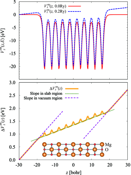
Figure 2: A slab (18 atoms per cell) is placed in in the middle of a supercell (60 a.u. width along the $z$ axis which is perpendicular to the slab), with electrodes at the left and right ends. At the top panel, we show $V_{z}^{\rm es}(z,E)$ for $E=0.2$ Ry and $E=0.0$ Ry. In the bottom panel, we show their difference $\Delta V_{z}^{\rm es}(z)$. From the ratio of two slopes of $\Delta V_{z}^{\rm es}$ in the slab region(green) and in the vacuum region(violet), we obtain $\epsilon_{\infty}({\rm Slab})$. We have better numerical accuracy by using $\Delta V_{z}^{\rm es}(z)$ instead of $V_{z}^{\rm es}(z,0.2{\rm Ry})$ directly.

In Fig.2, we illustrate our treatments in the slab models for five NaCl-structure ionic materials, where we use $\pm z_{0}=\pm 30$ a.u. We use slabs made of nine layers, 18 atoms in the supercell. We use experimental lattice constants of bulk materials, without relaxation of atomic positions. The electrostatic potential $V_{z}^{\rm es}(z,E)$ are the average of $V_{0}^{\rm es}({\bf r})$ in the xy plane under the bias voltage $E$. We plot the cases of $E=0.2$ Ry and of $E=0.0$ Ry. We show $\Delta V_{z}^{\rm es}(z)=V_{z}^{\rm es}(z,0.2{\rm Ry})-V_{z}^{\rm es}(z,0.0{\rm Ry})$ in the bottom panel in Fig.2. $\Delta V_{z}^{\rm es}(z,E)$ changes linearly as a function of $z$ in the vacuum regions and in the slab regions. From the ratio of two slopes of $\Delta V_{z}^{\rm es}$ in the slab region and in the vacuum region, we obtain $\epsilon_{\infty}({\rm Slab})$.

Table 1: Calculated optical dielectric constant $\epsilon_{\infty}$. ‘RPA’ are in bulk calculations with local field correction (LFC). ‘RPA(noLFC)’ are without LFC. ‘Slab’ are calculated from the slab models in the setting of Fig.2. Ratios $\eta=\frac{\epsilon_{\infty}({\rm RPA})}{\epsilon_{\infty}({\rm Slab})}$ and $\gamma=\frac{\epsilon_{\infty}({\rm Slab})-1}{\epsilon_{\infty}({\rm RPA})-1}$ are calculated just simply from the values of $\epsilon({\rm QSGW,RRA})$ and $\epsilon({\rm QSGW,Slab})$.

		RPA	RPA	Slab	$\eta$	$\gamma$	Experiments
		(noLFC)					Ashcroft et al. (2016); Sangster and Stoneham (1981); Jacobson and Nixon (1968)
LiF	GGA	2.04	1.95	2.01			1.96
	QSGW	1.73	1.67	1.94	0.86	1.40
KF	GGA	2.16	1.96	1.94			1.85
	QSGW	1.79	1.68	1.86	0.90	1.26
NaCl	GGA	2.70	2.33	2.42			2.34
	QSGW	2.13	1.92	2.31	0.83	1.42
MgO	GGA	3.17	2.96	3.09			2.96
	QSGW	2.50	2.37	2.91	0.81	1.39
CaO	GGA	3.94	3.59	3.68			3.33
	QSGW	2.88	2.68	3.31	0.81	1.38

Our main results are $\epsilon_{\infty}$ calculated from slab models in QSGW, $\epsilon_{\infty}({\rm QSGW,Slab})$, in Table 1. Note that $\epsilon_{\infty}({\rm Slab})$ contains the effect of vertex corrections based on QbP (See Sec.II), because changes of the self-energy caused by the bias $E$ are self-consistently taken into account. Numerical reliability of our calculations are estimated to be $\lesssim 1$ percent. See supplemental materials for computational details sup . In Table 1, we also show bulk values $\epsilon_{\infty}({\rm RPA})$. To obtain them, we first perform self-consistent calculations in QSGW for bulk materials. Then we calculate $\epsilon_{\infty}$ in the random-phase approximation (RPA) with/without local field correction (LFC). We also show $\epsilon_{\infty}$ in GGA together.

The QSGW values are in good agreements with experiments. For example, $\epsilon_{\infty}({\rm QSGW,Slab})$=1.94 for LiF gives surprisingly good agreement with $\epsilon_{\infty}({\rm Experiment})$=1.96.        In contrast, $\epsilon_{\infty}({\rm QSGW,RPA})$=1.67 is very smaller than $\epsilon_{\infty}({\rm QSGW,Slab})$=1.94. These are generally true in all other materials. We see that ratios $\eta=\epsilon_{\infty}({\rm QSGW,RPA})/\epsilon_{\infty}({\rm QSGW,Slab})$ in Table 1 are $\sim$0.8. This is consistent with Ref.Kotani et al., 2007 where $\epsilon_{\infty}$ for ZnO, Cu₂O, MnO, and NiO are presented. From a point of view to estimate the enhancement factors ($\approx$ vertex $\Gamma$ ) of the proper polarization, we may consider ratios $\gamma=\frac{\epsilon_{\infty}({\rm Slab})-1}{\epsilon_{\infty}({\rm RPA})-1}$. As shown in Table 1, $\gamma\sim$1.4. Since $\epsilon_{\infty}({\rm QSGW,Slab})$ gives very good agreements with $\epsilon_{\infty}({\rm experiment})$, we can say that the vertex correction for bulk should give the difference between $\epsilon_{\infty}({\rm RPA})$ and $\epsilon_{\infty}({\rm experiment})$ very well, where the vertex correction is calculated at the level of the functional derivative of the self-energy in QSGW; See Sec.III.

This is in contrast to the case of GGA. For example, look into the case of LiF. The difference $\epsilon_{\infty}({\rm GGA,Slab})-\epsilon_{\infty}({\rm GGA,RPA})=2.01-1.95=0.06$ is very small. The difference is originated from the xc kernel $f_{\rm xc}$ in the density functional perturbation theory. This is consistent with results in Ref.Botti et al., 2004 where they explicitly evaluate $f_{\rm xc}$ in GGA for bulk materials. Note that $\epsilon_{\infty}({\rm GGA,Slab})=2.01$ is a little larger than $\epsilon_{\infty}({\rm experiment})=1.96$; this is true for all other materials. We see that the contributions of vertex corrections $f_{\rm xc}$ do not necessarily improve agreements; $\epsilon_{\infty}({\rm GGA,Slab})$ give poorer agreement with $\epsilon_{\infty}({\rm experiment})$ than $\epsilon_{\infty}({\rm GGA,RPA})$.

IV.2 Rationale for QSGW80

Table 2: Calculated band gaps (eV) of bulk materials. In QSGW80, we show self-consistent results with the hybrid xc potential, 80 % QSGW+ 20 % GGA. QSGW80nosc specifies one-shot calculations with the hybrid potentials after QSGW 100% self-consistent calculations. QSGW80nosc is slightly larger because it is not fully self-consistent under such xc potential. See Ref.Deguchi et al., 2016.

	Experiments	QSGW	QSGW80	QSGW80nosc	GGA
	Roessler and Walker (1967a); Eby et al. (1959); Roessler and Walker (1967b); Whited et al. (1973)
LiF	13.6	16.04	14.53	14.85	9.52
KF	10.9	11.78	10.53	10.82	6.43
NaCl	8.6	9.51	8.55	8.76	5.37
MgO	7.77	8.86	7.91	8.10	4.86
CaO	7.1	7.45	6.57	6.74	3.69

Our result in Sec.IV.1 shows that the vertex correction should be included in the proper polarization $P$ to obtain $\epsilon_{\infty}$ in agreement with experiments. We have to use such $P$ in the QSGW self-consistent cycle. Such improved QSGW self-consistency can be identified as a self-consistent method in the $G_{0}W$ approximation on the basis of QbP. Ref.Shishkin et al., 2007 by Shishkin et al. gives a method on this idea.

However, their method is too expensive for computational efforts to apply wide-range of materials. In fact, although their method was applied to calculate ionization potentials in Ref.Grüneis et al., 2014, it was not so satisfactory because calculations are performed in the combination of simple materials (bulk calculations) with the supercell calculations in GGA. Furthermore, no papers available to treat transition-metal oxides such as LaMnO₃ in their method. We have to develop such an improved QSGW method applicable to wide range of materials. Two requirements are the computational efficiency and the theoretical validity.

As a possibility to respect the efficiency, we can consider a hybridization method between QSGW and the density functional xc Chantis et al. (2006). In QSGW80, a simple hybridization, 80 % QSGW+ 20 % GGA, we can see that it works well for wide range of materials. Our present results support the method of QSGW80, which takes only the 80 percent of QSGW self-energy. We can identify QSGW80 as a simplification of the method in Ref.Shishkin et al., 2007. Ref.Chen and Pasquarello, 2015 also presents one another approximation at the level of QSGW80 for the vertex correction in QSGW, resulting in similar good agreement with experiments.

Let us examine how QSGW80 is justified for materials calculated here. This is by the fact that $\eta=\epsilon_{\infty}({\rm QSGW,RPA})/\epsilon_{\infty}({\rm QSGW,Slab})$ in Table 1 are approximately 80 %, and show little material-dependency. Thus we expect that QSGW80 can mimic QSGW with the vertex corrections; too large screened-exchange effect is reduced by the factor 0.8, with adding 0.2 GGA term so as to keep the total size of the xc term. In Table 2, we show band gaps in QSGW and QSGW80 for materials treated here. The band gaps are systematically too large in QSGW in comparison with experimental values Deguchi et al. (2016), while QSGW80 gives rather better agreements with experimental values. In Ref.Deguchi et al., 2016, we checked the performance of the QSGW80 for ranges of materials. As in the case of Ref.Shishkin et al., 2007, QSGW80 is theoretically reasonable in the sense that the band gaps are improved by using the corrected $W$. To go beyond QSGW80, we have to develop methods to take the vertex correction into $W$ as was done in Ref.Shishkin et al., 2007 in a simple manner. Considering the fact that QSGW80 works well as shown in Ref.Deguchi et al., 2016, we may expect simple methods to represent the vertex correction by a scalar factor or by limited number of parameters. As long as we know, the vertex correction can be relatively insensitive to materials, thus we expect some simple method might be available.

V Summary

To clarify the importance of quasiparticle self-consistency in QSGW, we have explained the quasiparticle based perturbation in Sec.II. Then we emphasize the importance of the self-consistency in the $G_{0}W$ approximation. Then we obtain the quasiparticles (independent-particle) given by $H_{0}$, and the interaction between the quasiparticles given by $W$. The vertex correction in QbP is introduced.

We have performed QSGW calculations for slab models under electric field by means of the ESM method. The calculated $\epsilon_{\infty}$ are in good agreements with experimental values. Compared with $\epsilon_{\infty}$ in bulk calculation in RPA, we evaluated the size of vertex corrections as the functional derivative of the static self-energy in QSGW. Our results on $\epsilon_{\infty}$ give a support to the method by Shishkin, Marsman and Kresse Shishkin et al. (2007). As a simplified substitution of their method, we examined the performance of QSGW80 Deguchi et al. (2016) for materials treated here. The method QSGW+ESM developed for the calculations should be useful even for other purposes such as bias-dependent spin susceptibility in material theory, as well as practical device applications and materials designs.

To go beyond usual QSGW, we should develop improved QSGW method in the $G_{0}W$ approximation, whereas we should use accurate $W$ by including the vertex correction. Then we have virtually best division of $H=H_{0}+(H-H_{0})$ where $H_{0}$ gives the optimum independent particle picture.