Biomedical Image Segmentation by Retina-like Sequential Attention Mechanism Using Only A Few Training Images

Abstract

In this paper we propose a novel deep learning-based algorithm for biomedical image segmentation which uses a sequential attention mechanism able to shift the focus of attention across the image in a selective way, allowing subareas which are more difficult to classify to be processed at increased resolution. The spatial distribution of class information in each subarea is learned using a retina-like representation where resolution decreases with distance from the center of attention. The final segmentation is achieved by averaging class predictions over overlapping subareas, utilizing the power of ensemble learning to increase segmentation accuracy. Experimental results for semantic segmentation task for which only a few training images are available show that a CNN using the proposed method outperforms both a patch-based classification CNN and a fully convolutional-based method.

1 Introduction

Recently deep learning methods [2], which automatically extract hierarchical features capturing complex nonlinear relationships in the data, have managed to successfully replace most task-specific hand-crafted features. This has resulted in a significant improvement in performance on a variety of biomedical image analysis tasks, like object detection, recognition and segmentation (see e.g. [10] for a recent survey of the field and representative methods used in different applications), and currently Convolutional Neural Network (CNN) based methods define the state-of-the-art in this area.

In this paper we concentrate on biomedical image segmentation. For segmentation, where each pixel needs to be classified into its corresponding class, initially patch-wise training/classification was used [1]. In patch-based methods, local patches of pre-determined size are extracted from the images, typically using a CNN as pixel-wise classifier. During training, the patch is used as an input to the network and it is assigned as a label the class of the pixel at the center of the patch (available from ground-truth data provided by a human expert). During the test phase, a patch is fed into the trained net and the output layer of the net provides the probabilities for each class. More recently, Fully Convolutional Networks (FCN) [8], which replace the fully connected layers with convolutional ones, have replaced the patch-wise approach by providing a more efficient way to train CNNs end-to-end, pixels-to-pixels, and methods stemming from this approach presently define the state-of-the-art in biomedical image segmentation, exemplified by conv-deconv-based methods like U-Net [7].

Although fully convolutional methods have shown state-of-the-art performance on many segmentation tasks, they typically need to be trained on large datasets to achieve good accuracy. In many biomedical image segmentation tasks, however, only a few training images are available – either data simply being not available, or providing pixel-level ground truth by experts being too costly to obtain. Here we are motivated by a similar problem (section 3), where less than 50 images are available for training. On the other hand, patch-wise methods need only local patches, a huge number of which can be extracted even from a small number of training images. They however suffer from the following problem. While fully convolutional methods learn a map from pixel areas (multiple input image values) to pixel areas (multiple classes of all the pixels in the area), patch-wise methods learn a map from pixel areas (input image values) to a single pixel (class of the pixel in the center of the patch). As illustrated in Fig. 1 [i], this wastes the rich information about the topology of the class structure inside the patch for many of the samples which contain more than a single class, and these would typically be the most interesting/difficult samples [4]. Instead of trying to represent in a suitable way and learn the complex class topology, it just substitutes it by a single class (the class of the pixel in the center of the patch).

Regarding fully convolutional methods, they treat all locations in the images in the same way, which is in contrast with how human visual perception works. It is known that humans employ attentional mechanisms to focus selectively on subareas of interest and construct a global scene-representation by combining the information from different local subareas [6].

Figure 1: [i] Local patch containing pixels belonging to 3 classes shown in different color. On the right is normalized histogram showing the empirical distribution of the classes inside the patch, which can be interpreted as probabilities. A standard patch-wise method learns only the class of the pixel at the center, ignoring completely class topology. [ii] The proposed method learns the structure of the spatial distribution of the class topology in a local subarea represented similarly to the retina - the resolution is highest in the center and decreases progressively in the periphery. As attention shifts inside the image, the information of overlapping subareas is combined to produce the final segmented image (details explained in the text). Figure best viewed in color.

Based on the above observations, we propose a new method, which takes a middle ground between fully convolutional and patch-wise learning and combines the benefits of both of these strategies. As shown in Fig. 1, as in the patch-wise approach we consider subareas of the whole image at a time, which provides us with sufficient number of training samples, even if only a few ground-truth labeled images are available. However, as illustrated in Fig. 1 [ii], the class information is organized as in the retina [3]: the spatial resolution is highest in the central area (corresponding to the fovea), and it diminishes as we go to the periphery of the subarea. We propose a sequential attention mechanism which shifts the focus of attention in such a way that areas of the image which are difficult to classify (i.e. the classification uncertainty is higher) are considered in much more detail than areas which are easy to classify. Since the focus of attention moves the subarea under investigation much slower over difficult areas (i.e. with much smaller step), this results in many overlapping subareas in these regions. The final segmentation is achieved by averaging the class predictions over the overlapping subareas. In this way, the power of ensemble learning [5] is utilized by incorporating information from all overlapping subareas in the neighborhood (each of which provides slightly different views of the scene) to further improve accuracy.

This is the basic idea of the method proposed in the paper, and details how to implement it in a CNN will be given in the next section. Experimental results are reported in section 3, indicating that a significant improvement in segmentation accuracy can be achieved by the proposed method compared to both patch-based and fully convolutional-based methods.

2 Method

We represent a subarea $\cal{S}$ extracted from an input image (centered at the current focus of attention) as a tensor of size $d\times d\times c$, where $d$ is the size of the subarea in pixels and $c$ stands for the color channels if color images are used (as typically done, and $c=3$ for RGB images). As shown in Fig. 1 [ii], we can represent the class information corresponding to this subarea as grids of different resolution, where each cell in a grid contains a sample histogram $h^{(i)}$ calculated so that the $k$-th element of $h^{(i)}$ gives the number of pixels from class $k$ observed in the $i$-th cell of the grid. If each histogram $h^{(i)}$ is normalized to sum to 1 by dividing each bin by the total number of pixels covered by the cell, the corresponding vector $p^{(i)}$ can now be used to represent the probability mass function (pmf) for cell $i$: the $k$-th element of $p^{(i)}$, i.e. $p_{k}^{(i)}$, can be interpreted as the probability of observing class $k$ in the area covered by the $i$-th cell of the grid.

Next, we show how retina-like grids of different resolution levels can be created. Let’s start with a grid of size $4\times 4$, as shown in the top row of Fig. 1 [ii]. This we will call Resolution Level 1 and denote it as $r=1$. At resolution level 1 all the cells in the grid have the same resolution, i.e. the pmfs corresponding to each cell are calculated from areas of the same size. For example, if the size of the local subarea under consideration is $d=128$ pixels (i.e. image patch of size $128\times 128$ pixels), each cell in the grid at resolution level $r=1$ would correspond to an image area of size $32\times 32$ pixels from which a probability mass function $p^{(i)}$ would be calculated, as explained above. Next, we can create a grid at Resolution Level 2 ($r=2$) by dividing in half the four cells in the center of the grid, so that they form an inner $4\times 4$ grid, whose resolution is double. We can continue this process of dividing the innermost 4 cells into 2 to obtain still higher resolution levels. It is easy to see that the number of cells $N$ in a grid obtained at resolution level $r$ is $N=16+12(r-1)$. Of course, it is not necessary the initial grid at $r=1$ to be of size $4\times 4$, but choosing this number makes the process of creating different resolution levels especially simple, since in this case the innermost cells are always 4 ($2\times 2$).

In our method, we train a CNN to learn the map between a local subarea image given as input to the network, and the corresponding pmfs $p^{(i)}$ used as target values. We use the cross-entropy between the pmfs of the targets $p^{(i)}$ and the corresponding output unit activations $y^{(i)}$ as loss function $L$:

$$L=-\sum_{n}\sum_{i}\sum_{k}p^{(i)}_{k,n}\log{y^{(i)}_{k,n}}(S_{n};\vec{w}),$$ (1)

where $n$ indexes the training subarea image patches ($S_{n}$ being the $n$-th training subarea image patch), $i$ indexing the cells in the corresponding resolution grid, and $k$ the classes. Here, $\vec{w}$ represents the weights of the network, to be found by minimizing the loss function. To form probabilities, the network output units corresponding to each cell are passed through the soft-max activation function.

Finally, we describe the sequential attention mechanism we utilize, whose purpose is to move the focus of attention across the image in such a way that those parts which are difficult to classify (i.e. classification uncertainty is high) are observed at the highest possible resolution, and the retina-like grid of pmfs moves with smaller steps across such areas. To evaluate the classification uncertainty of the grid over the present subarea $\cal{S}$, we use the following function,

$$H(S)=-\frac{1}{N}\sum_{i\in S}\sum_{k}p^{(i)}_{k}\log{p^{(i)}_{k}},$$ (2)

which represents the average entropy obtained from the posterior pmfs $p^{(i)}$ for each cell (indexed by $i$) inside the grid, and $k$ indexes the classes. Using $H(S)$ as a measure of classification uncertainty, the position of the next location where to move the focus of attention (horizontal shift in pixels) is given by

$$f(H(S))=d\exp\{{-(H(S))^{2}/2\sigma^{2}}\}.$$ (3)

The whole process is illustrated in Fig. 2. We start at the upper left corner of the input image, with a subarea of size $d\times d$ pixels (the yellow patch (a) in the figure). The classification uncertainty for that subarea is calculated using Eq. 2, and the step size in pixels to move in the horizontal direction is calculated by Eq. 3. As illustrated in the graph in the center of Fig. 2, since in this case the classification uncertainty is 0 (all pixels in the subarea belong to the same class), the focus of attention moves $d$ pixels to the right, i.e. in this extreme case there is no overlap between the current and next subareas. For the subarea (b) shown in green, the situation is very different. In this case the classification uncertainty is very high, and the focus of attention would move only slightly to the right, allowing the image around this area to be assessed at the highest resolution. This would result in very high level of overlap between neighboring subareas, as shown in the heat map on the right (where intensity is proportional to the level of overlap). This process is repeated until the right corner of the image is reached. Then the focus of attention is moved 10 pixels in the vertical direction to scan the next row and everything is repeated until the whole image is processed.

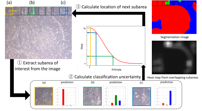
Figure 2: Overview of the sequential attention mechanism (see text for details).

While the above attention mechanism moves the focus of attention across the image, the posterior class pmfs from the grids corresponding to each subarea are stored in a probability map of the same size as the image, i.e. to each pixel in the image is allocated a pmf equal to the pmf of the cell from the grid positioned above that pixel. In areas in the image where several subareas overlap, the probability map is computed by averaging for each pixel the pmfs of all cells which partially overlap over that pixel. Finally, the class of the pixel is obtained by taking the class with highest probability from the final probability map, as shown in the upper right corner of Fig. 2 for the final segmented image.

Table 1: Experimental results for different values $d$ of the size of the local subareas

$d$	Method	Jaccard Index	Dice	TPR	TNR	Accuracy
96	patch-center	0.811 $\pm$ 0.039	0.879 $\pm$ 0.034	0.877 $\pm$ 0.039	0.922 $\pm$ 0.014	0.932 $\pm$ 0.016
	ResLv-1	0.798 $\pm$ 0.046	0.868 $\pm$ 0.040	0.866 $\pm$ 0.042	0.914 $\pm$ 0.016	0.928 $\pm$ 0.015
	ResLv-2	0.811 $\pm$ 0.037	0.879 $\pm$ 0.031	0.878 $\pm$ 0.035	0.919 $\pm$ 0.020	0.931 $\pm$ 0.015
	ResLv-3	0.819 $\pm$ 0.034	0.884 $\pm$ 0.029	0.883 $\pm$ 0.035	0.923 $\pm$ 0.012	0.936 $\pm$ 0.010
	ResLv-4	0.820 $\pm$ 0.033	0.884 $\pm$ 0.029	0.881 $\pm$ 0.036	0.926 $\pm$ 0.013	0.936 $\pm$ 0.012
UNet-patch	0.788 $\pm$ 0.051	0.861 $\pm$ 0.047	0.859 $\pm$ 0.045	0.916 $\pm$ 0.013	0.922 $\pm$ 0.011
128	patch-center	0.811 $\pm$ 0.029	0.878 $\pm$ 0.026	0.873 $\pm$ 0.028	0.917 $\pm$ 0.012	0.931 $\pm$ 0.012
	ResLv-1	0.812 $\pm$ 0.038	0.878 $\pm$ 0.032	0.874 $\pm$ 0.033	0.918 $\pm$ 0.020	0.935 $\pm$ 0.012
	ResLv-2	0.815 $\pm$ 0.039	0.881 $\pm$ 0.032	0.878 $\pm$ 0.034	0.923 $\pm$ 0.015	0.934 $\pm$ 0.014
	ResLv-3	0.816 $\pm$ 0.030	0.881 $\pm$ 0.029	0.879 $\pm$ 0.033	0.920 $\pm$ 0.011	0.935 $\pm$ 0.008
	ResLv-4	0.818 $\pm$ 0.034	0.821 $\pm$ 0.031	0.881 $\pm$ 0.031	0.921 $\pm$ 0.017	0.936 $\pm$ 0.011
	ResLv-5	0.826 $\pm$ 0.032	0.891 $\pm$ 0.030	0.890 $\pm$ 0.032	0.924 $\pm$ 0.018	0.936 $\pm$ 0.009
UNet-patch	0.810 $\pm$ 0.035	0.879 $\pm$ 0.030	0.873 $\pm$ 0.034	0.921 $\pm$ 0.014	0.933 $\pm$ 0.012
192	patch-center	0.778 $\pm$ 0.029	0.856 $\pm$ 0.025	0.849 $\pm$ 0.020	0.899 $\pm$ 0.017	0.917 $\pm$ 0.017
	ResLv-1	0.810 $\pm$ 0.037	0.876 $\pm$ 0.030	0.872 $\pm$ 0.031	0.914 $\pm$ 0.021	0.933 $\pm$ 0.016
	ResLv-2	0.817 $\pm$ 0.041	0.880 $\pm$ 0.038	0.879 $\pm$ 0.041	0.922 $\pm$ 0.017	0.936 $\pm$ 0.011
	ResLv-3	0.821 $\pm$ 0.032	0.885 $\pm$ 0.030	0.883 $\pm$ 0.032	0.926 $\pm$ 0.010	0.935 $\pm$ 0.011
	ResLv-4	0.832 $\pm$ 0.036	0.894 $\pm$ 0.030	0.890 $\pm$ 0.034	0.926 $\pm$ 0.015	0.940 $\pm$ 0.012
	ResLv-5	0.825 $\pm$ 0.032	0.887 $\pm$ 0.030	0.883 $\pm$ 0.032	0.925 $\pm$ 0.015	0.938 $\pm$ 0.012
UNet-patch	0.809 $\pm$ 0.036	0.878 $\pm$ 0.029	0.870 $\pm$ 0.034	0.920 $\pm$ 0.015	0.933 $\pm$ 0.015
256	patch-center	0.732 $\pm$ 0.038	0.822 $\pm$ 0.037	0.813 $\pm$ 0.039	0.862 $\pm$ 0.023	0.897 $\pm$ 0.019
	ResLv-1	0.804 $\pm$ 0.039	0.871 $\pm$ 0.035	0.866 $\pm$ 0.036	0.910 $\pm$ 0.018	0.931 $\pm$ 0.012
	ResLv-2	0.810 $\pm$ 0.038	0.877 $\pm$ 0.037	0.870 $\pm$ 0.040	0.918 $\pm$ 0.018	0.932 $\pm$ 0.012
	ResLv-3	0.819 $\pm$ 0.029	0.882 $\pm$ 0.028	0.879 $\pm$ 0.034	0.922 $\pm$ 0.016	0.937 $\pm$ 0.010
	ResLv-4	0.814 $\pm$ 0.033	0.877 $\pm$ 0.030	0.871 $\pm$ 0.031	0.917 $\pm$ 0.020	0.936 $\pm$ 0.011
	ResLv-5	0.815 $\pm$ 0.038	0.880 $\pm$ 0.034	0.876 $\pm$ 0.035	0.919 $\pm$ 0.016	0.934 $\pm$ 0.012
UNet-patch	0.811 $\pm$ 0.034	0.879 $\pm$ 0.028	0.874 $\pm$ 0.030	0.921 $\pm$ 0.014	0.933 $\pm$ 0.012
	UNet-image	0.806 $\pm$ 0.033	0.877 $\pm$ 0.029	0.874 $\pm$ 0.031	0.919 $\pm$ 0.013	0.928 $\pm$ 0.008

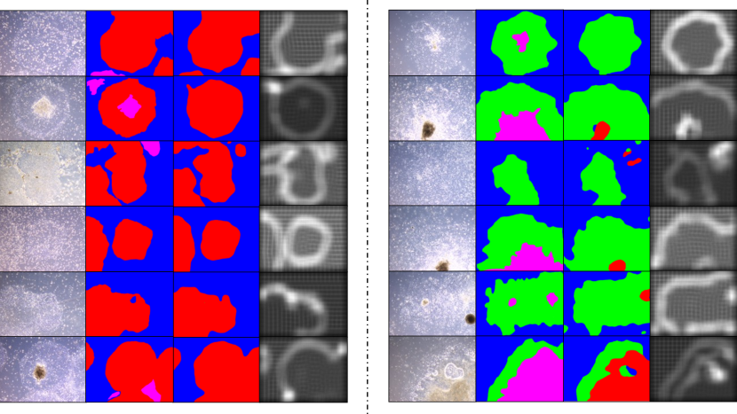
Figure 3: Segmentation results for several images from the iPS dataset, obtained by the proposed method (3rd column), using ResLv-4 with subarea size of $d=192$. First column shows the original images and second column the ground truth segmentation provided by an expert (red corresponds to class Good, green to Bad and blue to Background). The last column shows the corresponding heat map, where areas in which there was high overlap over neighboring subareas are shown with high intensity values.

3 Experiments

In this section we evaluate the proposed method in comparison with a standard patch-wise classification-based CNN [1] and the fully convolutional-based U-Net [7] on the dataset described below. Additionally we implemented a U-Net version, called UNet-patch, which applies U-Net to local patches rather than to a whole image. The original U-Net method which takes as input the whole image we will call UNet-image.
Dataset: Our dataset consists of 59 images showing colonies of undifferentiated and differentiated iPS cells obtained through phase-contrast microscopy. Induced pluripotent stem (iPS) cells [9], for whose discovery S. Yamanaka received the Nobel prize in Physiology and Medicine in 2012, contain great promise for regenerative medicine. Still, in order to fulfill their promise a steady supply of iPS cells obtained through harvesting of individual cell colonies is needed and automating the detection of abnormalities arising during the cultivation process is crucial. Thus, our task is to segment the input images into three categories: Good (undifferentiated), Bad (differentiated) and Background (BGD, the culture medium). Several representative images together with ground-truth provided by experts can be seen in Fig. 3. All images in this dataset are of size $1600\times 1200$ pixels. Several images contained a few locations where even the experts were not sure what the corresponding class was. Such ambiguous regions are shown in pink and these areas were not used during training and not evaluated during test.
Network Architecture and Hyperparameters: We used a network architecture based on the VGG-16 CNN net, apart from the following differences. There are 13 convolutional layers in VGG-16, while we used 10 here. Also, in VGG-16 there are 3 fully-convolutional layers of which the first two consist of 4096 units, while those had 1024 units in our implementation. The learning rate was set to 0.0001 and for the optimization procedure we used ADAM. Batch size was 16, training for 20 epochs (U-Net-patch for 15 epochs and U-Net-image for 200 epochs). For the implementation of the CNNs we used TensorFlow and Keras. Four different sizes for the local subareas were tried: $d=96,128,192,256$ and resolution level was changed between $r=1$ to $r=5$. The width of the Gaussian in Eq. 3 was empirically set to $\sigma=0.4$ for all experimental results. Evaluation procedure and criteria: The quality of the obtained segmentation results for each method were evaluated by 5-fold cross-validation using the following criteria: Jaccard index (the most challenging one), Dice coefficient, True Positive Rate (TPR), True Negative Rate (TNR) and Accuracy. For each score the average and standard deviation are reported.
Results: The results obtained on the iPS cell colonies dataset for each of the methods are given in Table 1, where, patch-center stands for the patch-wise classification method, and results for resolution levels from $r=1$ to $r=5$ are given for the proposed method. As can be seen from the results, the proposed method outperforms both patch-wise classification and the U-Net-based methods. Fig. 3 gives some examples of segmentation on images from the iPS dataset, showing that very good accuracy of segmentation can be achieved by the proposed method. The heat maps given in the last column demonstrate that the proposed attentional mechanism is able to focus the high-resolution parts of the retina-like grid on the boundaries between the classes which seem to be most difficult to classify, resulting in increased accuracy of segmentation.

4 Conclusion

In this paper we have shown that the combined power of (1) a sequential attention mechanism controlling the shift of the focus of attention, (2) local retina-like representation of the spatial distribution of class information and (3) ensemble learning can lead to increased segmentation accuracy in biomedical segmentation tasks. We expect that the proposed method can be especially useful for datasets for which only a few training images are available.

References

- [1] Cireşan, D.C., Giusti, A., Gambardella, L.M., Schmidhuber, J.: Deep neural networks segment neuronal membranes in electron microscopy images. In: NIPS. pp. 2843–2851 (2012)
- [2] Goodfellow, I., Bengio, Y., Courville, A.: Deep Learning. MIT Press (2016)
- [3] Kandel, E.R., Schwarz, J., Jessell, T.M., Siegelbaum, S.A., Hudspeth, A.J.: Principles of Neural Science, 5ed. McGraw-Hill (2013)
- [4] Kontschieder, P., Bulo, S.R., Bischof, H., Pelillo, M.: Structured class-labels in random forests for semantic image labeling. In: Proc. ICCV2012. pp. 2190 – 2197 (2012)
- [5] Kuncheva, L.: Combining Pattern Classifiers, 2ed. Wiley (2014)
- [6] Rensink, R.A.: The dynamic representation of scenes. Visual Cognition 7(1-3), 17–42 (2000)
- [7] Ronneberger, O., Fischer, P., Brox, T.: U-net: Convolutional networks for biomedical image segmentation. In: MICCAI (2015)
- [8] Shelhamer, E., Long, J., Darrell, T.: Fully convolutional networks for semantic segmentation. IEEE Trans. Pattern Anal. Mach. Intell. 39(4), 640–651 (2017)
- [9] Takahashi, K., Tanabe, K., Ohnuki, M., Narita, M., Ichisaka, T., Tomoda, K., Yamanaka, S.: Induction of pluripotent stem cells from adult human fibroblasts by defined factors. Cell 131 (5), 861–871 (2007)
- [10] Zhou, S.K., Greenspan, H., Shen, D. (eds.): Deep Learning for Medical Image Analysis. Academic Press (2017)