From Elastica to Floating Bodies of Equilibrium

Abstract

A short historical account of the curves related to the two-dimensional floating bodies of equilibrium and the bicycle problem is given. Bor, Levi, Perline and Tabachnikov found, quite a number had already been described as Elastica by Bernoulli and Euler and as Elastica under Pressure or Buckled Rings by Levy and Halphen. Auerbach already realized that Zindler had described curves for the floating bodies problem. An even larger class of curves solves the bicycle problem.

The subsequent sections deal with some supplemental details: Several derivations of the equations for the elastica and elastica under pressure are given. Properties of Zindler curves and some work on the problem of floating bodies of equilibrium by other mathematicians are considered. Special cases of elastica under pressure reduce to algebraic curves, as shown by Greenhill. Since most of the curves considered here are bicycle curves, a few remarks concerning them are added.

1 Introduction

Miklós Rédei introduces in his paper ”On the tension between mathematics and physics”[42] the ”supermarket picture” of the relation of mathematics and physics: that mathematics is like a supermarket and physics its customer.

When in 1938 Auerbach solved the problem of floating bodies of equilibrium[2] for the density $\rho=1/2$ he could go to the supermarket ’Mathematics’ and found the solution in form of the Zindler curves[63].

When I thought about this problem for densities $\rho\not=1/2$ I found a differential equation, went to the supermarket and found elliptic functions as ingredients for the solution. But in the huge supermarket I did not find the finished product. Later Bor, Levi, Perline, and Tabachnikov[7] showed me the shelf, where the boundary curves as Elastica under Pressure had been put already in the 19th century. The linear limit, which I had also considered had been put there as Elastica already in the 17th century by James Bernoulli[4, 5] and in the 18th century by Leonhard Euler.[14] Fortunately good mathematics has no date of expiry.

Section 2 presents a short historical survey of the curves and their applications, called Elastica and Elastica under Pressure or Buckled Rings. These curves, known since the seventeenth and nineteenth century, first as solutions of elastic problems, have shown up as solutions of quite a number of other problems, in particular as boundaries of two-dimensional bodies which can float in equilibrium in all orientations; this later problem is also solved by Zindler curves.

These classes of curves yield solutions to the bicycle problem. One asks in this problem for front and rear traces of a bicycle, which do not allow to conclude, in which direction the bicycle went, that is the traces are identical in both directions. The curves that give the traces of the front wheel and the traces of the rear wheels are the boundary and the envelope of the water lines, resp., of the floating bodies of equilibrium.

The subsequent sections deal with some supplemental details: In section 3 several derivations of the equations for the elastica and elastica under pressure are given. Section 4.1 deals with the Zindler curves and work on the problem of floating bodies of equilibrium by other mathematicians, including criticism. Section 5 is devoted to work by Greenhill, who found that special cases of the elastica under pressure can be represented by algebraic curves. Since most of the curves considered here are special cases of bicycle curves, section 6 brings some remarks on these curves.

2 Historical survey

In this paper we consider a class of planar curves, which surprisingly show up in quite a number of different physical and mathematical problems. These curves are not generally known, since they are represented by elliptic functions, although special cases can be represented by more elementary functions.

2.1 The Curves

These curves appear in two flavors; they obey in the linear form the equation

$$\frac{1}{\sqrt{1+y^{\prime 2}}}=ay^{2}+b$$ (1)

in Cartesian coordinates $(x,y=y(x))$, $y^{\prime}={\rm d}y/{\rm d}x$. The circular form is described by

$$\frac{1}{\sqrt{r^{2}+r^{\prime 2}}}=ar^{2}+b+\frac{c}{r^{2}},$$ (2)

in polar coordinates $(r,\phi)$ with $r=r(\phi)$ and $r^{\prime}={\rm d}r/{\rm d}\phi$. Eq. (1) yields the curvature $\kappa$,

$$\frac{1}{y^{\prime}}\frac{{\rm d}}{{\rm d}x}\frac{1}{\sqrt{1+y^{\prime 2}}}=-\frac{y^{\prime\prime}}{(1+y^{\prime 2})^{3/2}}=\kappa=2ay.$$ (3)

From (2) we obtain the curvature

$$\frac{1}{rr^{\prime}}\frac{{\rm d}}{{\rm d}\phi}\frac{r^{2}}{\sqrt{r^{2}+r^{\prime 2}}}=\frac{r^{2}+2r^{\prime 2}-rr^{\prime\prime}}{(r^{2}+r^{\prime 2})^{3/2}}=\kappa=4ar^{2}+2b.$$ (4)

We relate the polar coordinates to Cartesian coordinates and shift $y$ by $r_{0}$,

$$r\cos\phi=r_{0}+y,\quad r\sin\phi=x.$$ (5)

Then (4) reads

$$\kappa=4ar_{0}^{2}+8ar_{0}y+4a(x^{2}+y^{2})+b.$$ (6)

If we now choose

$$b=-2ar_{0}^{2},\quad a=\tilde{a}/(4r_{0}),$$ (7)

and perform the limit $r_{0}\rightarrow\infty$, then eq. (6) reads

$$\kappa=2\tilde{a}y,$$ (8)

which is the linear form (3). Thus the linear form is a limit of the circular form, where the radius $r_{0}$ goes to infinity.

The equation of the curves can be formulated coordinate-independent,

$$2\kappa^{\prime\prime}+\kappa^{3}-\mu\kappa-\sigma=0,$$ (9)

where the prime now indicates the derivative with respect to the arc length. Multiplication by $\kappa^{\prime}$ allows integration,

$$\kappa^{\prime 2}+\frac{\kappa^{4}}{4}-\mu\frac{\kappa^{2}}{2}-\sigma\kappa=2\hat{E}.$$ (10)

The coefficient $\sigma$ vanishes in the linear case. The derivation will become apparent, when we formulate the physical and/or mathematical problems solved by the curves. But the relation between eqs. (1, 2) and eqs. (9, 10) can also be given directly.[7]

2.2 Linear Elastica

The linear curves show up in Elastica. The question is: How does an elastic beam (or wire or rod) of given length bend? It may be fixed at two ends and the directions of the wire at both ends are given, or it is fixed at one end and loaded at the other end. Bending under load was already considered in the 13th century by Jordanus de Nemore, around 1493 by Leonardo da Vinci[3], in 1638 by Galileo Galilei, and in 1673 by Ignace-Gaston Pardies.[37, 53], although they could not give correct results.[37, 52] James Bernoulli following Hooke’s ideas obtained a correct differential equation assuming that the curvature is proportional to the bending moment, and partially solved it in 1691-1692. [4],

$$\frac{{\rm d}y}{{\rm d}x}=\frac{x^{2}}{\sqrt{a^{4}-x^{4}}}.$$ (11)

Huygens[31] argued in 1694 that the problem had a larger variety of solutions and sketched several of them. The more general differential equation was given by Bernoulli[5] in 1694-1695,

$$\frac{{\rm d}y}{{\rm d}x}=\frac{x^{2}\pm ab}{\sqrt{a^{4}-(x^{2}\pm ab)^{2}}},$$ (12)

This equation yields

$$\frac{1}{\sqrt{1+(\frac{{\rm d}x}{{\rm d}y})^{2}}}=\frac{x^{2}\pm ab}{a^{2}},$$ (13)

which is equation (1) with $x$ and $y$ exchanged and different notation for the constants. James Bernoulli also realized ”… among all curves of a given length drawn over a straight line the elastic curve is the one such that the center of gravity of the included area is the furthest distant from the line, just as the catenary is the one such that the center of gravity of the curve is the furthest distant …”[5]. Thus he found that the cross section of a volume of water contained in a cloth sheet is bounded (below the water line) by the elastica curve.

In 1742 Daniel Bernoulli (nephew of James) proposed in a letter to Leonhard Euler that the potential energy of a bent beam is proportional to the integral of the square of the curvature $\kappa$ integrated over the arclength $s$ of the beam $\int{\rm d}s\kappa^{2}$. In a 1744 paper Euler[14] used variation techniques to solve the problem. He found eq. (12), classified the solutions, discussed the stability, and realized that the curvature is proportional to $x$,

$$\kappa=\frac{y^{\prime\prime}}{(1+y^{\prime 2})^{3/2}}=\frac{2x}{a^{2}}.$$ (14)

This property plays a role in at least two other physical phenomena:

In 1807 Pierre Simon Laplace[36] investigated the shape of the capillary. The surface of a fluid trapped between two parallel vertical plates obeys also (14), since the difference of pressure inside and outside the fluid is proportional to the curvature of the surface.

Charges in a linearly increasing magnetic field move due to the Lorentz force on trajectories with curvature proportional to the magnetic field and thus again on trajectories given by the curves of elastica. Without being aware of this equivalence Evers, Mirlin, Polyakov, and Wölfle considered them in their paper on the semiclassical theory of transport in a random magnetic field.[15]

Figure 1: Examples of linear Elastica (i)

Figure 2: Examples of linear Elastica (ii)

Figure 3: Examples of linear Elastica (iii)

In 1859 Kirchhoff[33] introduced a kinetic analogue by showing that the problem of elastica is related to the movement of a pendulum. Set

$$\dot{x}=\cos\theta,\quad\dot{y}=\sin\theta,$$ (15)

where the dot indicates the derivative with respect to the arc $s$. Then one obtains

$$\dot{\theta}=\kappa,\quad y^{\prime}=\tan\theta.$$ (16)

Thus using eqs. (3) and (1) one obtains

$$\dot{\theta}^{2}=4a^{2}y^{2}=4a(\cos\theta-b).$$ (17)

Multiplication by $mr^{2}/2$ (with $m$ for the mass and $r$ for the length of the pendulum) and a corresponding choice of the constants $a$ and $b$, yields

$$\frac{mr^{2}}{2}\dot{\theta}^{2}-mgr\cos\theta=E.$$ (18)

This is the energy of a pendulum, if we substitute time $t$ for the arc $s$ in the derivative. Thus $\theta(t)$ is the time dependence of the angle of the pendulum against its lowest position. The periodic movement is obvious. Suppose $a$ is positive. Then for $-1<b<1$ the pendulum will swing in a finite interval $-\theta_{0}\leq\theta\leq+\theta_{0}$. These are the inflectional solutions. If $b<-1$ then the pendulum will move across the highest point $\theta=\pi$. These are the non-inflectional solutions. The limit case $b=-1$ yields a non-periodic solution (infinite period).

Some examples of elastica are shown in figures 1 to 3. The first two rows of figure 1 show non-inflectional cases where the pendulum moves across the highest point. The third row shows the aperiodic limit case $b=-1$. It is called syntractrix of Poloni (1729). The last row of figure 1 and figures 2 and 3 show inflectional cases corresponding to periodic oscillations without reaching the highest point. This yields a large variety of shapes including the Eight in the middle of figure 2 called lemnoid. The second drawing in figure 3 corresponds to the case where the pendulum moves up to a horizontal position. It is the rectangular elastica or right lintearia. The pendulum swings below the horizontal position in the last two rows of figure 3. In all cases the curves show equilibrium positions of the elastic beam. However, only sufficiently short pieces of the curves correspond to a stable equilibrium or even the absolute minimum of the potential energy.

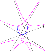
The hyperbolas are shown in magenta, their asymptotes in black. The vertices of the two branches are connected by a magenta line.

Figure 4: Rectangular elastica as roulette of hyperbola

Rectangular elastica as roulette of hyperbola The rectangular elastic curve is the locus of the center of a rectangular hyperbola rolling without slipping on a straight line. The upper branch of the hyperbola is shown in figure 4 in two different orientations. The midpoint between the branches lies on the blue rectangular linteria. (Sturm 1841, see [16], Greenhill 1892 [23]).

An excellent survey with many figures on the history of the elastica has been given by Raph Levien.[37] Also Todhunter[52] and Truesdell[53, 54] give reviews of the history of elasticity. Many details are found in the treatise by Love[39] on the mathematical theory of elasticity. In his PhD thesis[8] (1906) Max Born investigated elastic wires theoretically and experimentally in the plane and also in three dimensional space. The solution of eq. (1) or equivalently eqs. (11, 12) was given by Saalschütz[44] in 1880 by means of elliptic functions. The elliptic functions were developed by Abel and Jacobi mainly in the years 1826 – 1829 in several articles in Crelles Journal.[12]. Abel died in 1829, Jacobi published his fundamental work in the same year.[32] The explicit solutions are not given here. They can be found, e.g., in sect. 263 of [39], in sect. 13 of [37] and in ref. [60, 61]. Engineers often call ’Bernoulli-Euler beam theory’ approximations, in which the beam is only slightly bent.[62]

2.3 Elastica under Pressure (buckled rings)

By now we considered elastica to which only forces acted at the ends. A more general problem considers elastic wires, on which forces act along the arc. Maurice Levy realized in 1884[38] that the case, where a constant force $P$ per arc length acts perpendicularly on the wire, yields the differential equation (2). He showed that this problem could be solved by elliptic functions and found two types of solutions. They are called buckled rings, if the wire is closed. The constraints are equivalent if instead the perimeter and the area inside the ring are given. Halphen worked out the results in some detail in the same year[27] and included it in his ’Traité des fonctions elliptic et de leurs applications’.[28] Some elastica under pressure are shown in figure 5. Their symmetry is given by the dieder groups $D_{p}$ with $p=2,3,3$ in the first row, $p=4,4,5,5$ in the second row and $p=5,5,6$ in the third row. All of them are solutions of equation (2). Whereas those in the first and second row can be considered as deformed circles, those in the third row show double points. Similarly as for the elastica the curves show equilibrium configurations. But often only small parts of them are in stable equilibrium.

Figure 5: Examples of Elastica under Pressure (buckled rings)

Greenhill[24] considered the same problem in 1899 and looked particularly for curves that can be expressed by pseudo-elliptic functions. Thus some of the solutions are algebraic curves. The simplest example besides the circle is given by

$$r^{3}=a^{3}\cos(3\phi)$$ (19)

with the curvature

$$\kappa=4r^{2}/a^{3}$$ (20)

in polar coordinates $(r,\phi)$, which may be written

$$(x^{2}+y^{2})^{3}=a^{3}x(x^{2}-3y^{2})$$ (21)

in Cartesian coordinates $(x,y)$. This Kiepert curve (W. Roberts and L. Kiepert 1870, see [16]) looking like a cloverleaf is shown in fig. 6.

Figure 6: Kiepert curve $r^{3}=a^{3}\cos(3\phi)$

Area-constrained planar elastica in biophysics
Cells in biology have usually nearly constant volume and constant surface area. Their shape is to a large extend determined by the minimum of the membrane bending energy, see e.g. Helfrich[29] and Svetina and Zeks[49]. The two-dimensional analogue was considered by Arreaga, Capovilla et al.[1, 11] and by Goldin et al.[22]. Since pressure and area are conjugate quantities, the shapes are also given by those of elastica under pressure. Now of course, constant area and constant length of the bounding loop are given. The authors refer for the determination of the shape to the Lagrange equations (9, 10) as reported by Langer and Singer for elastica[35] and for buckled rings [34], see also the references [7, 47]. The equations for the elastica under pressure can also be obtained by considering the forces and momenta in the rods.[51] The solution of the equation (2) for buckled rings in terms of elliptic functions can be found in [38, 27, 28, 24] and in [60, 61]. Reference [61] contains further figures.

2.4 Floating Bodies of Equilibrium

2.4.1 Ulam’s Problem in two dimensions

The curves mentioned in the previous subsections appear in two other problems: the problem of Floating Bodies of Equilibrium and the Bicycle Problem. The first of these problems is related to the problem 19 in the Scottish Book by Ulam[55]: ”Is a solid of uniform density which will float in water in every position a sphere?” The two-dimensional version of the problem concerns a cylinder of uniform density $\rho$ which floats in water in equilibrium in every position with its axis parallel to the water surface. Sought is the curve different from a circle confining the cross section of the cylinder perpendicular to its axis.

The density of the log be $\rho$ (more precisely $\rho$ is the ratio of the density of the log over that of the liquid). The area of the cross section be $A$, the part above and below the water-line are denoted by $A_{1}$ and $A_{2}$. Then Archimedes’ law requires

$$A_{1}=(1-\rho)A,\quad A_{2}=\rho A.$$ (22)

The distance of the center of gravity of the cross section above the water-line be $h_{1}$, that below the water-line $h_{2}$, the length of the log $L$. Then the potential energy is

$$\rho(1-\rho)ALg(h_{1}+h_{2}).$$ (23)

Thus $h_{1}+h_{2}$ has to be constant. The line connecting the two centers of gravity has to be perpendicular to the water-line. Rotation by an infinitesimal angle yields that the length $2l$ of the water-line obeys

$$\frac{2}{3}l^{3}\left(\frac{1}{A_{1}}+\frac{1}{A_{2}}\right)=h_{1}+h_{2}.$$ (24)

Thus the length of the water-line does not depend on the orientation of the log. The conditions that the area below the water-line and the length of the water-line are constant implies that the part of the perimeter of the cross-section below the water-line is constant. It also implies that the envelope of the water-lines is given by the midpoints of the water-lines.

This two-dimensional problem has attracted many mathematicians.

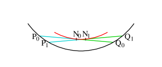
Figure 7: Lower part of the boundary (black) of the floating body

Two waterlines $P_{0}Q_{0}$ and $P_{1}Q_{1}$ are in blue and cyan. The midpoints $N_{0}$ and $N_{1}$ lie on the envelope (red) of the water-lines.

2.4.2 Density $\rho=1/2$

There is a large class of solutions for $\rho=1/2$. The solutions are not related to the elastica, but it seems worthwhile to mention them. Basically the solutions were found by Zindler[63], although he did not consider this physical problem, but found convex curves which have the property that chords between two points on the boundary which bisect the perimeter have constant length $2l$ and simultaneously cut the enclosed area in two halves. They can be parameterized by

$$x(\alpha)=l\cos(\alpha)+\xi(\alpha), y(\alpha)=l\sin(\alpha)+\eta(\alpha),$$ (25)

$$\xi(\alpha)=\int^{\alpha}{\rm d}\beta\cos(\beta)\hat{\rho}(\beta), \eta(\alpha)=\int^{\alpha}{\rm d}\beta\sin(\beta)\hat{\rho}(\beta),$$ (26)

with parameter $\alpha$, where $\xi$ and $\eta$ obey

$$\xi(\alpha+\pi)=\xi(\alpha),\quad\eta(\alpha+\pi)=\eta(\alpha).$$ (27)

$(\xi,\eta)$ are the coordinates of the envelope of the water lines, and $|\hat{\rho}(\alpha)|$ is the radius of curvature of the envelope. Typically the envelope has an odd number of cusps.

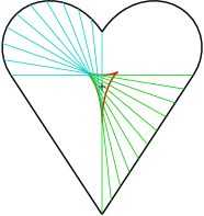
Figure 8: Heart-shaped Zindler curve, see Auerbach[2]

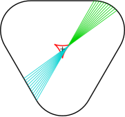
Figure 9: Zindler curve, see Auerbach[2]

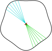
Figure 10: Zindler curve, five-fold symmetry

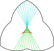
Figure 11: Zindler curve, see Salgaller and Kostelianetz[45], similarly by Zindler[63]

Condition (27) implies $\hat{\rho}(\beta+\pi)=-\hat{\rho}(\beta)$. The chords run from $(x(\alpha),y(\alpha))$ to $(x(\alpha+\pi),y(\alpha+\pi))$. Zindler did not consider the centers of gravity of both halfs of the area. Otherwise he would have realized that their distance does not depend on the angle $\alpha$ and the line between them is always perpendicular to the chord. This class of curves was also found by Auerbach[2] in 1938 and by Geppert[19] in 1940. Special cases were given by Salkowski[46] in 1934 and by Salgaller and Kostelianetz[45] in 1939. Examples of Zindler curves are shown in figures 9 to 11. They are due to Auerbach[2], Zindler[63], and Salgaller and Kostelianetz[45]. The envelopes of the water lines are shown in red, the water lines in blue and cyan.

2.4.3 Density $\rho\not=$ 1/2

For a long time it was not clear, whether solutions for $\rho\not=1/2$ exist. Gilbert[21] in his nice article ’How things float’ claims in section 3 ’Different heart-shaped cross sections work for other densities (he means densities different from $1/2$) and there are other solutions that are not heart-shaped.’ Indeed, there are cross-sections that are not heart-shaped for density 1/2 and densities different from 1/2. But I do not know a heart-shaped solution for density different from 1/2 and I doubt that at the time he wrote the paper a solution for densities different from 1/2 was known. At least he does not give reference to such a solution.

Attempts to find solutions for $\rho\not=1/2$ by Salkowski[46] in 1934, Gericke[20] in 1936, and Ruban[43] in 1939 failed. As I will explain later, it seems that Ruban was close to a solution. It was proven by several authors that chords, which form a triangle or a quadrangle yield only circles.

Bracho, Montejano, and Oliveros[9, 10, 41] were probably the first to find solutions for densities different from $1/2$. They consider a carousel, which is a dynamical equilateral polygon in which the midpoint of each edge travels parallel to it. The trace of the vertices describe the boundary and the midpoints outline the envelope of the waterline. In this way they found solutions where the chords form an equilateral pentagon. However, their solutions were not sufficiently convex, since the water line cuts the cross section in some positions several times.

For special densities $\rho$ one can deform the circular cross-section into one with $p$-fold symmetry axis and mirror symmetry.

$$r(\phi)=r_{0}(1+2\epsilon\cos(p\phi)+2\sum_{n=2}^{\infty}c_{n}\cos(pn\phi)),$$ (28)

where the coefficients $c_{n}$ are functions of $\epsilon$ and $p$ with $c_{n}=O(\epsilon^{n})$. The corresponding $p-2$ densities depend on $\epsilon$. Surprisingly, the perturbation expansion in $\epsilon$ yielded (up to order $\epsilon^{7}$) one and the same solution for all $p-2$ densities, although it had to be expected only for pairs with density $\rho$ and $1-\rho$. The present author reported this result in [58]. This result was unexpected. It was probably true to all orders in $\epsilon$ and thus deserved further investigation. (In eq. (83) of [58]v3 $c_{\delta_{0}}$ should be replaced by $s_{\delta_{0}}$).

In a first step the limit $p\rightarrow\infty$ was considered with $r_{0}\propto p$ and $\epsilon\propto 1/p$. This corresponds to the transition from the circular case to the linear case mentioned in subsection 2.1. In this limit only terms $\sum_{n,k}c_{n,k}p^{n+2k-1}\epsilon^{n+2k}\cos(pn\phi)$ in the expansion (28) contribute (with odd $n$).

Property of constant distance These curves have a remarkable property, which I call the property of constant distance:

Consider two copies of the curves. Choose an arbitrary point on each curve. Then in the linear case there exists always a length $\delta u$ by which the curves can be shifted against each other, and in the circular case there exists an angle $\delta\phi$ by which the two curves can be rotated against each other, so that the distance $2l$ between the two points stays constant, if they move on both curves by the same arc distance $s$.

Considering this procedure the other way round, we may shift curves in the linear case continuously against each other and watch how the distance $2l$ increases with $\delta u$, or we may rotate the curves in the circular case continuously against each other and watch how $2l$ varies with $\delta\phi$. When $\delta\phi$ is increased by $2\pi/p$, then both curves fall unto themselves, and a solution for the floating bodies is found, provided the curve is sufficiently convex, so that the chord between the two points does not intersect the curve at another point.

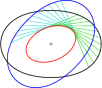
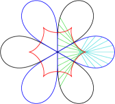
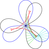
Figure 12: Property of constant distance

The first figure of 5 and figure 6 are shown in two copies rotated against each other by $45^{0}$, $60^{0}$ and $30^{0}$.

In figure 12 three examples for the property of constant distance are shown. Two copies of the first of the figures 5 are shown in black and blue. The lines of constant distance $2l$ are drawn in cyan and green switching color in the middle, where they touch the red envelope. Similarly these lines are shown for copies of the Kiepert curve, figure 6, rotated against each other by $\delta\phi=60^{0}$ and $\delta\phi=30^{0}$, resp. The length $2l$ of the chord for the Kiepert curve is given by $2l=a|\sin(3\delta\phi/2)|^{1/3}$.

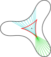
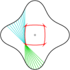
Figure 13: Floating bodies of equilibrium, $p=3$ and $p=4$

The distance $2l$ shrinks for the buckled ring (first figure of figure 12) after rotation by $2\pi/p=180^{0}$ to zero. Therefore it cannot serve as floating body of equilibrium. The buckled rings in figure 13 of symmetry $D_{3}$ and $D_{4}$ and those in figure 14 of symmetry $D_{5}$ are boundaries of floating bodies of equilibrium. Rotation by $2\pi/p$ yields a non-zero distance $l$. The waterlines are shown in green and cyan, the envelope of the waterlines in red. The figures with odd $p$ are also solutions for $\rho=1/2$, thus special Zindler curves. The figures with $p=5$ are besides solutions for $\rho=1/2$ also solutions for a density $\rho>1/2$ and for a density $\rho<1/2$.

Figure 14: Floating bodies of equilibrium, $p=5$

We turn to the linear case with examples in figure 15. In the first to third row examples of figures from the second to fourth row of figure 1 are shown. They are shifted by a distance $\delta u$ and in one case one curve is reflected. This reflected curve is solution of eq. 1 with the same constants $a$ and $b$. In the fourth and fifth row two examples are shown, where the figures were shifted so far that they fall on each other, together with lines of length $2l$ and the envelopes.

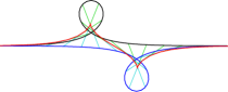
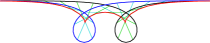
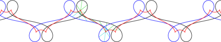
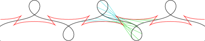
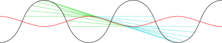
Figure 15: Property of constant distance for the linear case

The derivation of the differential equations (2,1) for the curves are contained in [57] based on [58, 59]. First the linear case was dealt with, where first large distances, then infinitesimal distances, and finally arbitrary distances were considered (section 2 of [59]). It yields eq. (1) (Eq. (17) of [59] and Eq. (27) of [57]). The circular case is considered in section 3 of [59] and in section 3.2 of [57]. In deriving this equation the author assumed that also for non-integer periodicity $p$ such chords (of infinitesimal length) exist between the curves rotated against each other by nearly $2\pi$. This assumption yields a differential equation of order 3, (43) of [59] and (33) of [57]. It can be integrated easily to eq. (2) (Eq. (47) of [59] and Eq. (37) of [57]). Explicit solution of these equations showed that the property of constant distance holds.[60, 61]

The problem is originally non-local, since it connects end-points of the chords generally without the necessecity of closing them to a polygon of chords. The eqs. (1, 2), however, reduce it to a local problem: The equations connect only locus and direction of the curve at the same point.

It came to my big surprise, when Bor, Levine, Perline, and Tabachnikov[7] pointed out, that the problem of elastica under pressure and the problem of floating bodies of equilibrium in two dimensions are governed by the same differential equation (2).

Charges in magnetic fields The curvature of the boundary curves is quadratic in the radius $r$, $\kappa=4ar^{2}+2b$ according to eq. (4). Thus charges moving in a perpendicular magnetic field of such an r-dependence, will move along these curves.

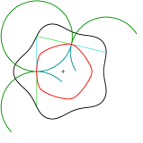
Figure 16: Magnetic billiard for perpendicular incidence

The red boundary is given by the envelope of the chords.

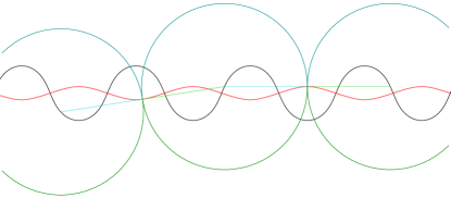
Figure 17: Magnetic billiard for perpendicular incidence

The red boundary is given by the envelope of the chords.

A different system is a dynamical billiard. There a particle alternates between free motion and specular reflections at a boundary (angle of incidence equals angle of reflection). Circles are boundaries with the property that the particle leaves and arrives at the boundary at the same angle $\delta$. Gutkin[25] found boundaries of billiards with this property, but different from circles.

In a magnetic billiard the particle is charged and subject to a constant perpendicular magnetic field. Thus it does not move on straight lines, but on Larmor circles of radius $R$ given by its charge and mass, and by the strength of the magnetic field. If the angle $\delta$ with the boundary of the billiard is a right angle, then billiards bounded by the (red) envelopes of the chords have this Gutkin $\delta$ property, if the radius equals half the length of the chords, $R=l$. (Bialy, Mironov, and Shalom[6]). These Larmor arcs can be inside (shown in dark blue), but also outside the boundary, (shown in dark green) in figure 17. Such Larmor arcs are also possible at the envelopes of the chords of linear elastica, see figure 17.

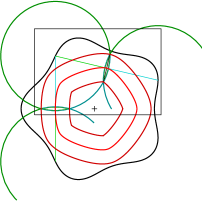
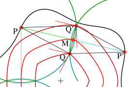
Figure 18: Magnetic billiards for $\delta\not=90^{0}$

The dark red parallel curves are the boundaries of the billiards. Right figure: Cut-out.

If the particle does not meet the boundary at right angle, then the boundary is described by a parallel curve to the envelope. These parallel curves are shown in figure 18 in dark red. The chord $PP^{\prime}$ touches the red envelope at the midpoint $M$. The parallel curves and the Larmor circles go through $Q$ and $Q^{\prime}$. The tangents at these curves at $Q$ and $Q^{\prime}$ are indicated by red lines. The angle between the tangents at $Q$ be $\delta$, that at $Q^{\prime}$ is $\delta^{\prime}$. Both angles add up to $180^{0}$. The angles in the rhomb $PQP^{\prime}Q^{\prime}$ with midpoint $M$ obey $\angle Q^{\prime}PM=\angle QPM=\angle Q^{\prime}P^{\prime}M=\angle QP^{\prime}M=90^{0}-\delta$. It is now obvious that the radius of the Larmor arcs obey $l=R\sin\delta$ and the distance between the red envelope and the boundaries of the billiards is $R\cos\delta$.

This construction is restricted to angles $\delta$ sufficiently close to $90^{0}$ and envelopes sufficiently convex.[6] Obviously the boundaries are not allowed to have double points.

2.5 The Bicycle Problem

The bicycle problem is closely related to the problem of finding floating bodies of equilibrium. It was addressed by Finn[17, 18, 50]. The problem goes back to a criticism of the discussion between Sherlock Holmes and Watson in The Adventure of the Priory School[13] on which way a bicycle went whose tires’ traces are observed. Let the distance between the front and the rear wheel of the bicycle be $l$. The end points of the tangent lines of length $l$ to the trace of the rear wheel in the direction the bicycle went yields the points of the traces of the front wheel. Thus if the tangent lines in both directions end at the trace of the front wheel, it is open which way the bicycle went. Thus curves $\gamma$ for the rear wheel (in red in Fig. 7) and $\Gamma$ for the front wheel (in black in fig. 7) are solutions for such an ambiguous direction of the bicycle. The tire track problem consists in finding such curves $\Gamma$ and $\gamma$ different from the trivial solutions of circles and straight lines.

Obviously the solutions of the two-dimensional floating body problem solve the bicycle problem, but also the linear elastica and the Zindler curves solve the problem. There are more solutions to the bicycle curves. Finn argues that the variety of bicycle curves is much larger: Draw from one point ($N_{0}$) of the rear tire track the tangent to the front wheel in both directions and give an arbitrary smooth tire track between these two points ($P_{0}$) and ($Q_{0}$) in figure 7. Then one can continue tire track curves in both directions.[17, 18].

We shortly explain why Zindler curves are bicycle curves. Let the bicyclist go in one direction so that the front wheel is at $(x(\alpha),y(\alpha))$ given in eq. (25) and with the rear wheels at $(\xi(\alpha).\eta(\alpha))$. Then the bicyclist going in the opposite direction is with its front wheels at

$$x_{-}(\alpha)=-l\cos(\alpha)+\xi(\alpha),\quad y_{-}(\alpha)=-l\sin(\alpha)+\eta(\alpha).$$ (29)

Since $(x_{-}(\alpha),y_{-}(\alpha))=(x(\alpha+\pi),y(\alpha+\pi))$ and the traces of the rear wheels agree due to (27), both bicyclists use the same traces for their wheels and one cannot determine, which way the bicyclist went.

Zindler curves, but also a number of curves from elastica and buckled rings yield envelopes, that is traces of the rear wheels with cusps. Then the rear wheel has to go back and forth. For these curves the front wheel has to be turned by more than the right angle. Driving along these traces requires artistic skills and a suitable bicycle. Apart from the Zindler curves (figs. 9 to 11) this is the case for the first, second, and fourth buckled ring of figure 13, the inner rear trace of figure 14, and the elastica of the fourth row of fig. 15. However, the third traces of fig. 13, the outer trace of fig. 14, and the traces of the fifth row of fig. 15 can be easily traversed. They constitute good solutions of the bicycle problem.

3 Derivation of the differential equations

The equations governing the elastic beam (wire) have been given in different ways. They are developed in this section. These differential equations have been given in numerous papers apart from their original derivation in numerous papers. I mention only [7, 34, 35, 37, 39, 47, 48, 51] and references therein.

3.1 Bernoulli - Huygens solution

James Bernoulli considered initially a beam AB loaded by a weight C at the end assuming the beam to be horizontally at the point of the load, see figure 19.

Figure 19: Beam AB with load C

He assumed the curvature $\kappa$ to be a function $f$ of the moment. Hence,

$$\kappa=\frac{{\rm d}\phi}{{\rm d}s}=\frac{{\rm d}}{{\rm d}x}\frac{y^{\prime}}{\sqrt{1+y^{\prime 2}}}=f(x),$$ (30)

where $\phi$ is the angle of the tangent at the curve against the x-axis. Integration yields

$$y^{\prime}=\frac{S(x)}{\sqrt{1-S^{2}(x)}},\quad S(x)=\int_{0}^{x}{\rm d}\xi f(\xi).$$ (31)

Assuming a linear relation between the curvature and the moment gives

$$f(x)=\frac{2x}{a^{2}},\quad S(x)=\frac{x^{2}\pm ab}{a^{2}}$$ (32)

and thus equation (12). The rectangular elastica primarily considered by James Bernoulli is obtained for $b=0$.

3.2 Forces and Pressure

Here we consider the force and torque acting in the elastic wire similar to that given by Levy[38] and derive eqs. (3, 4). Let us cut out a piece from ${\bf r}$ to ${\bf r}^{\prime}$ (figure 20). At the ends act forces ${\bf F}$ and $-{\bf F}^{\prime}$. In addition a force per length $P$ perpendicular to the wire exerts the force

$${\bf F}_{P}=P{\bf e}_{3}\times({\bf r}^{\prime}-{\bf r})$$ (33)

on the piece of wire, where ${\bf e}_{3}$ is the unit vector perpendicular to the plane.

Figure 20: Wire, forces, torques, pressure, and tangent and normal vectors

The total force vanishes in the static case,

$${\bf F}-{\bf F}^{\prime}+P{\bf e}_{3}\times({\bf r}^{\prime}-{\bf r})=0.$$ (34)

Integration yields the force acting on the wire,

$${\bf F}({\bf r})={\bf F}_{0}+P{\bf e}_{3}\times{\bf r}.$$ (35)

Next we consider the torque acting on the piece of wire. Due to the curvature of the wires there are torques ${\bf M}$ and $-{\bf M}^{\prime}$ at the ends of the wires. Moreover ${\bf r}\times{\bf F}$ and $-{\bf r}^{\prime}\times{\bf F}^{\prime}$ are exerted by the forces at the ends and the force on the piece exerts

$${\bf M}_{P}=\int{\rm d}{\bf M}_{P}=\int(-{\bf r}\times{\rm d}{\bf F}_{P})=-P\int{\bf r}\times({\bf e}_{3}\times{\rm d}{\bf r})$$

$$=-P\int{\bf e}_{3}({\bf r}{\rm d}{\bf r})=-\frac{1}{2}P{\bf e}_{3}(r^{\prime 2}-r^{2}).$$ (36)

The total torque vanishes,

$${\bf M}-{\bf M}^{\prime}+{\bf r}\times{\bf F}-{\bf r}^{\prime}\times{\bf F}^{\prime}+{\bf M}_{P}=0.$$ (37)

This yields

$${\bf M}({\bf r})=-{\bf r}\times{\bf F}_{0}-\frac{1}{2}P{\bf e}_{3}r^{2}+{\bf M}_{0}.$$ (38)

Let us introduce

$${\bf M}={\bf e}_{3}M,\quad{\bf M}_{0}={\bf e}_{3}M_{0},\quad{\bf e}_{3}\times{\bf F}_{0}={\bf F}_{n}.$$ (39)

Multiplication of (38) by ${\bf e}_{3}$ yields

$$M({\bf r})={\bf r}\cdot{\bf F}_{n}-\frac{1}{2}Pr^{2}+M_{0}=-\frac{1}{2}P({\bf r}-\frac{{\bf F}_{n}}{P})^{2}+\frac{{\bf F}_{n}^{2}}{2P}+M_{0}.$$ (40)

The torque is proportional to the curvature $\kappa$

$$M=-EI\kappa,$$ (41)

where $E$ is the elastic modulus and $I$ the second moment with respect to the axis in $e_{3}$-direction through the center of gravity of the cross section of the wire. Love calls this the ordinary approximate theory and discusses it in sections 255 – 258 of his book.[39]

If there is no external force, $P=0$, then the first equation (40) yields

$$\kappa=-\frac{1}{EI}({\bf r}\cdot{\bf F}_{n}+M_{0})$$ (42)

in agreement with eq. (3). Hence $\kappa$ increases linearly with ${\bf r}$ parallel to ${\bf F}_{n}$.

If $P\not=0$, then we replace ${\bf r}-{\bf F}_{n}/P\rightarrow{\bf r}$ and obtain

$$\kappa=4ar^{2}+2b,\quad a=P/(8EI),\quad b=-({\bf F}^{2}_{n}/(2P)+M_{0})/(2EI).$$ (43)

Hence the curvature $\kappa$ increases quadratically with ${\bf r}$ in accordance with eq. (4).

3.3 Equation for the curvature

We start with the Frenet-Serret formula for the tangential vector ${\bf t}$ and the normal vector ${\bf n}$ of the wire

$$\frac{{\rm d}{\bf t}}{{\rm d}s}=\kappa{\bf n},\quad\frac{{\rm d}{\bf n}}{{\rm d}s}=-\kappa{\bf t}.$$ (44)

We express the force as

$${\bf F}=F_{t}{\bf t}+F_{n}{\bf n}.$$ (45)

Then going along the wire (beam) we obtain

$$\frac{{\rm d}}{{\rm d}s}(F_{t}{\bf t}+F_{n}{\bf n})=P{\bf n}.$$ (46)

Thus

$$\frac{{\rm d}F_{t}}{{\rm d}s}-\kappa F_{n}=0,$$ (47)

$$\frac{{\rm d}F_{n}}{{\rm d}s}+\kappa F_{t}=P.$$ (48)

The torque obeys

$$\frac{{\rm d}M}{{\rm d}s}=-F_{n}.$$ (49)

Finally the torque is assumed to be proportional to the curvature

$$M=-EI\kappa.$$ (50)

This yields

$$EI\frac{{\rm d}\kappa}{{\rm d}s}=F_{n}.$$ (51)

We insert this relation in eq. (47) and obtain

$$\frac{{\rm d}F_{t}}{{\rm d}s}-EI\kappa\frac{{\rm d}\kappa}{{\rm d}s}=0,$$ (52)

which can be integrated to

$$F_{t}-\frac{EI}{2}\kappa^{2}=c^{\prime}.$$ (53)

Equations (51) and (48) yield

$$EI\frac{{\rm d}^{2}\kappa}{{\rm d}s^{2}}=\frac{{\rm d}F_{n}}{{\rm d}s}=-\kappa F_{t}+P=\kappa(-c^{\prime}-\frac{EI}{2}\kappa^{2})+P.$$ (54)

Hence

$$\frac{{\rm d}^{2}\kappa}{{\rm d}s^{2}}+\frac{1}{2}\kappa^{3}+\frac{c^{\prime}}{EI}\kappa-\frac{P}{EI}=0.$$ (55)

If we multiply this equation by ${\rm d}\kappa/{\rm d}s$ and integrate, then we obtain

$$\frac{1}{2}\left(\frac{{\rm d}\kappa}{{\rm d}s}\right)^{2}+\frac{1}{8}\kappa^{4}+\frac{c^{\prime}}{2EI}\kappa^{2}-\frac{P}{EI}\kappa=\hat{E}.$$ (56)

These are the equations (9) and (10).

3.4 Geometrical derivation

In this subsection we will derive this equation requiring the extreme of the integral over the square of the curvature with appropriate side conditions. We perform a purely geometrical derivation. As a function of the arc parameter $s$ we introduce the angle $\phi$ of the tangent against the x-axis and the Cartesian coordinates. The origin is at $s=0$. The curve starts with the angle $\phi_{0}$.

$$\phi(s) = \phi_{0}+\int_{0}^{s}{\rm d}s^{\prime}\kappa(s^{\prime}),$$ (57)

$$x(s) = \int_{0}^{s}{\rm d}s^{\prime}\cos(\phi(s^{\prime})),$$ (58)

$$y(s) = \int_{0}^{s}{\rm d}s^{\prime}\sin(\phi(s^{\prime})).$$ (59)

The length of the arc be $s_{0}$. The area between the arc and the straight line from the origin to the endpoint of the arc $(x(s_{0}),y(s_{0}))$ is given by

$$A=\frac{1}{2}\int_{0}^{s_{0}}{\rm d}s(x(s)\sin(\phi(s))-y(s)\cos(\phi(s))).$$ (60)

We may have several side conditions on the curve: the angle at the end point $\phi(s_{0})$, the coordinates of the end point and the area fixed. Thus the corresponding quantities have to be subtracted from the integral over $\kappa^{2}/2$ by Lagrange multipliers $\lambda_{1}...\lambda_{5}$,

$$I=\frac{1}{2}\int_{0}^{s_{0}}{\rm d}s\kappa^{2}(s)-\lambda_{1}\phi(s_{0})-\lambda_{2}x(s_{0})-\lambda_{3}y(s_{0})-\lambda_{4}A-\frac{\lambda_{5}}{2}(x^{2}(s_{0})+y^{2}(s_{0})).$$ (61)

In total these may be too many conditions. But for those we do not take into account, we set $\lambda_{i}=0$. The variation of $I$ has to vanish,

$$\delta I = \int_{0}^{s_{0}}{\rm d}s\delta\kappa(s)F(s),$$ (62)

$$F(s) = \kappa(s)-\lambda_{1}+(\lambda_{2}+\lambda_{5}x(s_{0}))\int_{s}^{s_{0}}{\rm d}s^{\prime}\sin(\phi(s^{\prime}))$$

$$- (\lambda_{3}+\lambda_{5}y(s_{0}))\int_{s}^{s_{0}}{\rm d}s^{\prime}\cos(\phi(s^{\prime}))$$

$$- \frac{\lambda_{4}}{2}\int_{s}^{s_{0}}{\rm d}s^{\prime}(x(s^{\prime})\cos(\phi(s^{\prime}))+y(s^{\prime})\sin(\phi(s^{\prime})))$$

$$+ \frac{\lambda_{4}}{4}\left(\int_{s}^{s_{0}}{\rm d}s^{\prime}\sin(\phi(s^{\prime}))\right)^{2}+\frac{\lambda_{4}}{4}\left(\int_{s}^{s_{0}}{\rm d}s^{\prime}\cos(\phi(s^{\prime}))\right)^{2}$$

$$= \kappa(s)-\lambda_{1}+\lambda_{2}(y(s_{0})-y(s))-\lambda_{3}(x(s_{0})-x(s))$$

$$+ \frac{\lambda_{4}}{2}[x(s)(x(s)-x(s_{0}))+y(s)(y(s)-y(s_{0}))]$$

$$+ \lambda_{5}(x(s_{0})y(s)-y(s_{0})x(s)).$$ (64)

The equation $F(s)=0$ has to be solved.One immediately sees from eq. (64) that $\kappa$ depends (for $\lambda_{4}\not=0$) quadratically on the distance from some point. The derivatives of $F$ with respect to $s$, indicated by a dot vanish,

$$\dot{F}(s) = \dot{\kappa}(s)+K_{1}=0,$$ (65)

$$K_{1} = \cos(\phi(s))[\lambda_{3}+\lambda_{4}x(s)-\frac{\lambda_{4}}{2}x(s_{0})-\lambda_{5}y(s_{0})]$$ (66)

$$+ \sin(\phi(s))[-\lambda_{2}+\lambda_{4}y(s)-\frac{\lambda_{4}}{2}y(s_{0})+\lambda_{5}x(s_{0})],$$

$$\ddot{F}(s) = \ddot{\kappa}(s)+K_{2}\kappa+\lambda_{4}=0,$$ (67)

$$K_{2} = -\sin(\phi(s))[\lambda_{3}+\lambda_{4}x(s)-\frac{\lambda_{4}}{2}x(s_{0})-\lambda_{5}y(s_{0})]$$ (68)

$$+ \cos(\phi(s))[-\lambda_{2}+\lambda_{4}y(s)-\frac{\lambda_{4}}{2}y(s_{0})+\lambda_{5}x(s_{0})],$$

$$\stackrel{{\scriptstyle\mbox{...}}}{{F}}(s) = \stackrel{{\scriptstyle\mbox{...}}}{{\kappa}}(s)+K_{2}\dot{\kappa}(s)-K_{1}\kappa(s)^{2}=0.$$ (69)

Elimination of $K_{1}$ and $K_{2}$ yields

$$\kappa\dot{F}(s)-\frac{1}{\kappa^{2}}\dot{\kappa}\ddot{F}(s)+\frac{1}{\kappa}\stackrel{{\scriptstyle\mbox{...}}}{{F}}(s)=\kappa\dot{\kappa}-\frac{1}{\kappa^{2}}\dot{\kappa}\ddot{\kappa}-\frac{\lambda_{4}}{\kappa^{2}}\dot{\kappa}+\frac{1}{\kappa}\stackrel{{\scriptstyle\mbox{...}}}{{\kappa}}=0.$$ (70)

This expression is a complete derivative. Integration and multiplication by $\kappa$ gives

$$\frac{1}{2}\kappa^{3}+\ddot{\kappa}+\lambda_{4}+C_{1}\kappa=0.$$ (71)

This is the Lagrange equation for the relative extrema of the bending energy. Multiplication of this expression by $\dot{\kappa}$ and another integration yields

$$\frac{1}{2}\dot{\kappa}^{2}+\frac{1}{8}\kappa^{4}+\lambda_{4}\kappa+\frac{C_{1}}{2}\kappa^{2}=C_{2},$$ (72)

which agrees with eqs. (55) and (56) by renaming the constants. Apart from eq. (70) also boundary conditions for $F=0$, $\dot{F}=0$, and $\ddot{F}(0)$ at $s=0$ or $s=s_{0}$ have to be fulfilled. Thus $\kappa$, $\dot{\kappa}$, and $\ddot{\kappa}$ at $s=0$ or $s=s_{0}$ are expressed by $\lambda_{i}$ and $x(s_{0})$, $y(s_{0})$, $\phi$ at $s=0$ or $s=s_{0}$. Insertion in (71) and (72) yields the corresponding constants $C_{1}$ and $C_{2}$.

3.5 Water contained in a cloth sheet

James Bernoulli showed that water contained in a long cloth sheet (in y-direction) is bound in the xz-direction by an elastic curve. (See Levien[37], footnotes 3 and 5, and Truesdell[53], p. 201). This problem goes under the name of lintearia.

The cloth ends should be fixed at $(\xi_{1},\zeta_{1})$ and $(\xi_{2},\zeta_{2})$. The height of the water-line is $h$. The water surface ranges from $x_{1}$ to $x_{2}$ as in figures 22 and 22.

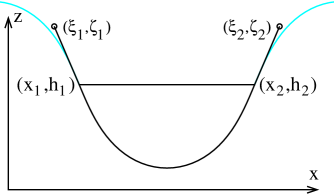
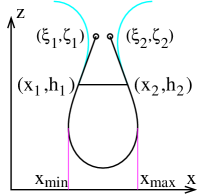
Figure 21: Cross section of the cloth filled with water for $x_{1}>\xi_{1}$ and $x_{2}<\xi_{2}$.

Figure 22: Cross section of the cloth filled with water for $x_{1}<\xi_{1}$ and $x_{2}>\xi_{2}$.

The cyan curve indicates in both cases the continuation of the elastica curve.

We give two derivations, a longer one using variational techniques, and a shorter one, considering forces and pressure as in subsection 3.3.

3.5.1 Variation of the potential energy

We denote the area of the cross section by $A$, the breadth of the cloth by $s$, the potential energy by $V$, the length of the cloth in y-direction $L_{y}$, the gravitational constant $g$, and the density of the water $\rho$. Then the area of the cross section $A$, the potential energy $V$ and the breadth $s$ of the cloth are given by

$$A = \int_{x_{1}}^{x_{2}}{\rm d}x(h(x)-z(x)),$$ (73)

$$V = \frac{L_{y}g\rho}{2}\int_{x_{1}}^{x_{2}}{\rm d}x(h^{2}(x)-z^{2}(x)),$$ (74)

$$s = s_{1}+s_{2}+s_{3},$$ (75)

$$s_{1} := \sqrt{(\xi_{1}-x_{1})^{2}+(\zeta_{1}-h_{1})^{2}},$$ (76)

$$s_{2} := \sqrt{(\xi_{2}-x_{2})^{2}+(\zeta_{2}-h_{2})^{2}},$$ (77)

$$s_{3} := \int_{x_{1}}^{x_{2}}{\rm d}x\sqrt{1+z^{\prime 2}},$$ (78)

$$z^{\prime} := \frac{{\rm d}z}{{\rm d}x},\quad h^{\prime}:=\frac{{\rm d}h}{{\rm d}x}.$$ (79)

Of course we know that $h(x)$ does not depend on $x$. However, it is of advantage to have $h(x_{1})$ and $h(x_{2})$ as two variables, which can be varied independently.

We look for the extreme of $V-\alpha A-\sigma S$. The variations are

$$\delta A = \int_{x_{1}}^{x_{2}}{\rm d}x(\delta h(x)-\delta z(x)),$$ (80)

$$\delta V = L_{y}g\rho\int_{x_{1}}^{x_{2}}{\rm d}x(h\delta h-z\delta z),$$ (81)

$$\delta s_{1} = \frac{\delta x_{1}(x_{1}-\xi_{1})+\delta h_{1}(h_{1}-\zeta_{1})}{s_{1}},$$ (82)

$$\delta s_{2} = \frac{\delta x_{2}(x_{2}-\xi_{2})+\delta h_{2}(h_{2}-\zeta_{2})}{s_{2}},$$ (83)

$$\delta s_{3} = \delta x_{2}\sqrt{1+z_{2}^{\prime 2}}-\delta x_{1}\sqrt{1+z_{1}^{\prime 2}}+\int_{x_{1}}^{x_{2}}{\rm d}x\frac{z^{\prime}}{\sqrt{1+z^{\prime 2}}}\frac{{\rm d}\delta z}{{\rm d}x},$$ (84)

$$z^{\prime}_{i} := z^{\prime}(x=x_{i}),\quad h^{\prime}_{i}:=h^{\prime}(x=x_{i}).$$ (85)

We have not included contributions proportional to $\delta x_{i}$ in $\delta A$ and $\delta V$, since $h_{i}=z_{i}$ at $x_{i}$. Partial integration transforms the integral to

$$\int_{x_{1}}^{x_{2}}{\rm d}x\frac{z^{\prime}}{\sqrt{1+z^{\prime 2}}}\frac{{\rm d}\delta z}{{\rm d}x}=\delta z_{2}\frac{z^{\prime}_{2}}{\sqrt{1+z_{2}^{\prime 2}}}-\delta z_{1}\frac{z^{\prime}_{1}}{\sqrt{1+z_{1}^{\prime 2}}}-\int_{x_{1}}^{x_{2}}{\rm d}x\delta z\frac{{\rm d}}{{\rm d}x}\left(\frac{z^{\prime}}{\sqrt{1+z^{\prime 2}}}\right).$$ (86)

The variation of $V-\alpha A-\sigma S$ contains contributions proportional to $\delta x_{i},\delta h_{i}$, and $\delta z_{i}$ and an integral over $x$,

$$\int_{x_{1}}^{x_{2}}{\rm d}x(L_{y}g\rho h(x)-\alpha)\delta h(x)$$ (87)

$$- \int_{x_{1}}^{x_{2}}{\rm d}x\left(L_{y}g\rho z(x)-\alpha-\sigma\frac{{\rm d}}{{\rm d}x}\left(\frac{z^{\prime}}{\sqrt{1+z^{\prime 2}}}\right)\right)\delta z(x)$$ (88)

The variation of $\delta h(x)$ yields constant $h$ as expected,

$$\alpha=L_{y}g\rho h.$$ (89)

The variation of $\delta z(x)$ yields

$$L_{y}g\rho(z(x)-h)=\sigma\frac{{\rm d}}{{\rm d}x}\left(\frac{z^{\prime}}{\sqrt{1+z^{\prime 2}}}\right)=\sigma\frac{z^{\prime\prime}}{(1+z^{\prime 2})^{3/2}}=\sigma\kappa.$$ (90)

Thus the curvature increases proportional to the depth measured from the water-surface.

Since the variation of $h(x_{i})=z(x_{i})$ yields

$$\delta h_{i}+h^{\prime}_{i}\delta x_{i}=\delta z_{i}+z^{\prime}_{i}\delta x_{i},\quad\delta z_{i}=\delta h_{i}-z^{\prime}_{i}\delta x_{i},$$ (91)

we obtain the contributions

$$\delta x_{1}\left(\frac{x_{1}-\xi_{1}}{s_{1}}\mp\frac{1}{\sqrt{1+z_{1}^{\prime 2}}}\right)+\delta h_{1}\left(\frac{h-\zeta_{1}}{s_{1}}\mp\frac{z_{1}^{\prime}}{\sqrt{1+z_{1}^{\prime 2}}}\right)$$ (92)

$$+ \delta x_{2}\left(\frac{x_{2}-\xi_{2}}{s_{2}}\pm\frac{z_{2}^{\prime}}{\sqrt{1+z_{2}^{\prime 2}}}\right)+\delta h_{2}\left(\frac{h-\zeta_{2}}{s_{2}}\pm\frac{z_{2}^{\prime}}{\sqrt{1+z_{2}^{\prime 2}}}\right).$$

The factors of $\delta x_{i}$ and $\delta h_{i}$ have to vanish. They yield the direction of the lines from the lines of the suspension to the lines where the cloth touches the waterline. If $x_{1}>\xi_{1}$ and $\xi_{2}>x_{2}$ as in fig. 22, then the upper signs in (92) apply, and the slope is continuous across the waterline as expected.

If instead $x_{1}<\xi_{1}$ and $\xi_{2}<x_{2}$ as in fig. 22, then $z(x)$ is double-valued with values $z_{-}(x)$ and $z_{+}(x)$. Then the $x$-integral of $s_{3}$ reads

$$s_{3}=\int_{x_{\rm min}}^{x_{\rm max}}{\rm d}x\sqrt{1+z_{-}^{\prime 2}(x)}+\int_{x_{\rm min}}^{x_{1}}{\rm d}x\sqrt{1+z_{+}^{\prime 2}(x)}+\int_{x_{2}}^{x_{\rm max}}{\rm d}x\sqrt{1+z_{-}^{\prime 2}(x)}.$$ (93)

Accordingly the contributions from $s_{3}$ change sign and the lower signs in (92) apply. Again the slope is continuous across the waterline. The expression for the area and similarly for the potential have different signs in front of the integrals,

$$A=\int_{x_{\rm min}}^{x_{\rm max}}{\rm d}x(h(x)-z_{-}(x))-\int_{x_{\rm min}}^{x_{1}}{\rm d}x(h(x)-z_{+}(x))-\int_{x_{2}}^{x_{\rm max}}{\rm d}x(h(x)-z_{+}(x)).$$ (94)

3.5.2 Considering forces and pressure

A simpler derivation can be given by considering the forces and the pressure as in subsection 3.3.

Since the cloth can be bent without exerting any forces or torques, one has $F_{n}=0$, $M=0$, $c=0$. Thus eqs. (47) and (48) read

$$\frac{{\rm d}F_{t}}{{\rm d}s}=0,\quad\kappa\frac{F_{t}}{L_{y}}=P,$$ (95)

where $F_{t}$ is the total force over the length $L_{y}$. The pressure acts from inside and depends on $z$,

$$P=-\rho g(h-z).$$ (96)

This yields

$$F_{t}={\rm const},\quad\kappa=\frac{L_{y}\rho g(z-h)}{F_{t}}$$ (97)

in agreement with equation (3).

3.6 Elastica as roulette of Hyperbola

We determine the differential equation for the roulette of the hyperbola. We parametrize the coordinates $(x_{h},y_{h})$ of the hyperbola by a parameter $p$,

$$x_{h}=a\cosh(p), y_{h}=b\sinh(p),$$ (98)

$$\frac{{\rm d}x_{h}}{{\rm d}p}=a\sinh(p), \frac{{\rm d}y_{h}}{{\rm d}p}=b\cosh(p).$$ (99)

$a$ and $b$ are the semi axes of the hyperbola. The arc length $s$ of the hyperbola reads

$${\rm d}s=-\sqrt{q}{\rm d}p,\quad q=a^{2}\sinh^{2}(p)+b^{2}\cosh^{2}(p)=\frac{a^{2}+b^{2}}{2}\cosh(2p)+\frac{b^{2}-a^{2}}{2}.$$ (100)

The coordinates $(x,y)$ of the midpoint between the branches of the hyperbola rolling on the x-axis without slipping obey

$$\left(\begin{array}[]{c}x\\ y\end{array}\right)=\left(\begin{array}[]{c}s\\ 0\end{array}\right)+\frac{1}{\sqrt{q}}\left(\begin{array}[]{cc}a\sinh(p)&b\cosh(p)\\ -b\cosh(p)&a\sinh(p)\end{array}\right)\left(\begin{array}[]{c}x_{h}\\ y_{h}\end{array}\right),$$ (101)

which yields

$$x=s+\frac{a^{2}+b^{2}}{2\sqrt{q}}\sinh(2p),\quad y=-\frac{ab}{\sqrt{q}}.$$ (102)

The derivatives

$$\frac{{\rm d}x}{{\rm d}p}=\frac{a^{2}b^{2}}{q^{3/2}},\quad\frac{{\rm d}y}{{\rm d}p}=\frac{ab(a^{2}+b^{2})}{2q^{3/2}}\sinh(2p)$$ (103)

yield

$$\frac{{\rm d}y}{{\rm d}x}=\frac{a^{2}+b^{2}}{2ab}\sinh(2p).$$ (104)

We express $\sinh(2p)$ by $q$ and $q$ by $y$,

$$q=\left(\frac{ab}{y}\right)^{2},\quad\left(q+\frac{a^{2}-b^{2}}{2}\right)^{2}=\left(\frac{a^{2}+b^{2}}{2}\sinh(2p)\right)^{2}+\left(\frac{a^{2}+b^{2}}{2}\right)^{2}.$$ (105)

This yields the differential equation for the Sturm roulette for the hyperbola rolling on a straight line

$$\frac{{\rm d}y}{{\rm d}x} = \frac{1}{ab}\sqrt{\left(q+\frac{a^{2}-b^{2}}{2}\right)^{2}-\left(\frac{a^{2}+b^{2}}{2}\right)^{2}}=\frac{1}{ab}\sqrt{(q+a^{2})(q-b^{2})}$$ (106)

$$= \frac{1}{ab}\sqrt{\left(\frac{a^{2}b^{2}}{y^{2}}+a^{2}\right)\left(\frac{a^{2}b^{2}}{y^{2}}-b^{2}\right)}=\frac{1}{y^{2}}\sqrt{(b^{2}+y^{2})(a^{2}-y^{2})}.$$

For a rectangular hyperbola one has $b=a$ and this equation reduces to

$$\frac{{\rm d}y}{{\rm d}x}=\frac{\sqrt{a^{4}-y^{4}}}{y^{2}},$$ (107)

which is eq. (11) for the rectangular elastica, only the coordinates $x$ and $y$ exchanged.

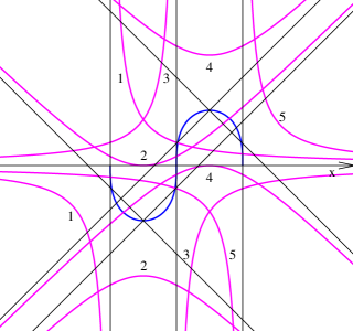
The hyperbolas are depicted in magenta, the asymptotes in black, and the elastica in blue.

Figure 23: Full period of the rectangular elastica as roulette of hyperbola

The roulette shown in figure 4 shows only half a period of the rectangular elastica. One obtains the full period, if one first rolls the upper branch of the hyperbola, as shown in figure 23 starting with hyperbola 1 over hyp. 2 to hyp. 3, where for 1 and 3 one asymptote is along the x-axis. Now we roll the lower branch from hyp. 3 to 4 and 5. This yields the second half of the elastica. The hyperbola 5 has the same orientation as number 1, only shifted by one period along the x-axis. Now one may continue for another period, and so on.

4 The case $\rho=1/2$

The boundaries of the two-dimensional floating bodies of equilibrium with density $1/2$ are Zindler curves. We describe these closed curves in the following subsection. Chords of the curves bisect both the boundary and the enclosed area. The centers of gravity of these halves have constant distance and their connecting line is perpendicular to the chord (subsect. 4.2). In the following subsection 4.3 I comment on some papers which investigate plain regions with the property that chords of constant length cut the region in two pieces of constant areas. Some of them deal with the problem of floating bodies of equilibrium, others are purely geometrical.

4.1 Zindler curves

Zindler considers mainly in sects. 6, 7 and 10 of [63] convex plain areas with the property that any chord between two points bisecting the perimeter has constant length and bisects the area.

The envelope of the chords is defined by Equation (26) with the constraint (27) which implies $\xi(\pi)=\xi(0)$, $\eta(\pi)=\eta(0)$. The boundary can be parameterized by equation (25). Hence

$$x(\alpha+\pi)=\xi(\alpha)-l\cos(\alpha),\quad y(\alpha+\pi)=\eta(\alpha)-l\sin(\alpha).$$ (108)

The diameters $D(\alpha)$ ranges from $(x(\alpha),y(\alpha))$ to $(x(\alpha+\pi),y(\alpha+\pi))$. It bisects the perimeter and the area enclosed by the boundary, provided $l$ is sufficiently large, so that the diameters cut the boundary only at the end points of the diameter.

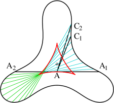
Figure 24: Two halves of the area

The area is cut in halves by the diameter $D(\alpha)=A_{1}AA_{2}$. The coordinates of $A$ are $\xi(\alpha),\eta(\alpha)$, and those of $A_{1},A_{2},C_{1},C_{2}$ are (x,y) at $\alpha,\alpha+\pi,\gamma,\gamma+{\rm d}\gamma$, resp. The infinitesimal triangle of eq. (109) is $AC_{1}C_{2}$.

We consider now the two regions cut by the diameter $D(\alpha)$. They consist of infinitesimal triangles $AC_{1}C_{2}$, (fig. 24)

$$A=(\xi(\alpha),\eta(\alpha)),\quad C_{1}=(x(\gamma),y(\gamma)),\quad C_{2}=(x(\gamma+{\rm d}\gamma),y(\gamma+{\rm d}\gamma)),$$ (109)

with $\gamma=\alpha_{1}=\alpha...\alpha+\pi$ for region 1 and $\gamma=\alpha_{2}=\alpha-\pi...\alpha$ for region 2.

Then the perimeter is given by

$$u_{1,2}=\int_{\alpha_{1,2}}^{\alpha_{1,2}+\pi}{\rm d}\gamma\sqrt{x^{\prime}(\gamma)^{2}+y^{\prime}(\gamma)^{2}}=\int_{\alpha_{1,2}}^{\alpha_{1,2}+\pi}{\rm d}\gamma\sqrt{\hat{\rho}^{2}(\gamma)+l^{2}}.$$ (110)

Since $\hat{\rho}(\gamma-\pi)=-\hat{\rho}(\gamma)$, one obtains the same integral. Hence $u_{2}=u_{1}$. The diameter bisects the perimeter.

The area of the infinitesimal triangle (109) is given by

$${\rm d}A=\frac{1}{2}{\rm d}\gamma[(x(\gamma)-\xi(\alpha))y^{\prime}(\gamma)-(y(\gamma)-\eta(\alpha))x^{\prime}(\gamma)].$$ (111)

With the abbreviations

$$\xi_{\gamma,\alpha}:=\xi(\gamma)-\xi(\alpha),\quad\eta_{\gamma,\alpha}:=\eta(\gamma)-\eta(\alpha)$$ (112)

we obtain

$$x(\gamma)-\xi(\alpha) = l\cos(\gamma)+\xi_{\gamma,\alpha},$$

$$y(\gamma)-\eta(\alpha) = l\sin(\gamma)+\eta_{\gamma,\alpha},$$

$$x^{\prime}(\gamma) = -l\sin(\gamma)+\hat{\rho}(\gamma)\cos(\gamma),$$

$$y^{\prime}(\gamma) = l\cos(\gamma)+\hat{\rho}(\gamma)\sin(\gamma)$$ (113)

and

$${\rm d}A = \frac{1}{2}{\rm d}\gamma[l^{2}+l\xi_{\gamma,\alpha}\cos(\gamma)+l\eta_{\gamma,\alpha}\sin(\gamma)$$ (114)

$$+ \xi_{\gamma,\alpha}\hat{\rho}(\gamma)\sin(\gamma)-\eta_{\gamma,\alpha}\hat{\rho}(\gamma)\cos(\gamma)].$$

One finds that both areas $A_{1}$ and $A_{2}$ are equal

$$A_{1}=A_{2} = \frac{\pi}{2}l^{2}-\Delta,$$

$$\Delta = \int_{\alpha}^{\alpha+\pi}{\rm d}\gamma\eta(\gamma)\hat{\rho}(\gamma)\cos(\gamma)$$ (115)

$$= -\int_{\alpha}^{\alpha+\pi}{\rm d}\gamma\xi(\gamma)\hat{\rho}(\gamma)\sin(\gamma).$$

They are independent of $\alpha$, since the integrand is a periodic function of $\gamma$ with period $\pi$. The term proportional to $l$ vanishes, since it is a total derivative of a function, which vanishes at the limits,

$$\int_{\alpha_{1,2}}^{\alpha_{1,2}+\pi}{\rm d}\gamma[\xi_{\gamma,\alpha}\cos(\gamma)+\eta_{\gamma,\alpha}\sin(\gamma)]$$ (116)

$$= \int_{\alpha_{1,2}}^{\alpha_{1,2}+\pi}{\rm d}\gamma\frac{{\rm d}}{{\rm d}\gamma}[\xi_{\gamma,\alpha}\sin(\gamma)-\eta_{\gamma,\alpha}\cos(\gamma)].$$

4.2 Centers of Gravity

Zindler did not consider the centers of gravity of the two half areas. It is important for the floating body problem that their distance is constant and that the straight line between the two centers is normal to the chord.

The centers of gravity $(\bar{x}(\gamma),\bar{y}(\gamma))$ of the infinitesimal triangles (109) are given by

$$\bar{x}(\gamma) = \frac{1}{3}\xi(\alpha)+\frac{2}{3}(l\cos(\gamma)+\xi(\gamma))=\xi(\alpha)+\frac{2}{3}(l\cos(\gamma)+\xi_{\gamma,\alpha}),$$

$$\bar{y}(\gamma) = \frac{1}{3}\eta(\alpha)+\frac{2}{3}(l\sin(\gamma)+\eta(\gamma))=\eta(\alpha)+\frac{2}{3}(l\sin(\gamma)+\eta_{\gamma,\alpha}).$$ (117)

Thus the centers of gravity $(\bar{X},\bar{Y})$ of the halves of the area are given by the integrals

$$A_{1,2}\bar{X}_{1,2}(\alpha) = \int{\rm d}A\bar{x}=\int{\rm d}A\xi(\alpha)+\frac{1}{3}\int{\rm d}\gamma[l^{3}\cos(\gamma)$$ (118)

$$+ l^{2}\xi_{\gamma,\alpha}(1+\cos^{2}(\gamma))+l^{2}\eta_{\gamma,\alpha}\cos(\gamma)\sin(\gamma)$$

$$+ l\xi_{\gamma,\alpha}^{2}\cos(\gamma)+l\xi_{\gamma,\alpha}\eta_{\gamma,\alpha}\sin(\gamma)$$

$$+ l\xi_{\gamma,\alpha}\hat{\rho}(\gamma)\sin(\gamma)\cos(\gamma)-l\eta_{\gamma,\alpha}\hat{\rho}(\gamma)\cos^{2}(\gamma)$$

$$+ \xi_{\gamma,\alpha}^{2}\hat{\rho}(\gamma)\sin(\gamma)-\xi_{\gamma,\alpha}\eta_{\gamma,\alpha}\hat{\rho}(\gamma)\cos(\gamma)],$$

$$A_{1,2}\bar{Y}_{1,2}(\alpha) = \int{\rm d}A\bar{y}=\int{\rm d}A\eta(\alpha)+\frac{1}{3}\int{\rm d}\gamma[l^{3}\sin(\gamma)$$ (119)

$$+ l^{2}\xi_{\gamma,\alpha}\cos(\gamma)\sin(\gamma)+l^{2}\eta_{\gamma,\alpha}(1+\sin^{2}(\gamma))$$

$$+ l\xi_{\gamma,\alpha}\eta_{\gamma,\alpha}\cos(\gamma)+l\eta_{\gamma,\alpha}^{2}\sin(\gamma)$$

$$+ l\xi_{\gamma,\alpha}\hat{\rho}(\gamma)\sin^{2}(\gamma)-l\eta_{\gamma,\alpha}\hat{\rho}(\gamma)\sin(\gamma)\cos(\gamma)$$

$$+ \xi_{\gamma,\alpha}\eta_{\gamma,\alpha}\hat{\rho}(\gamma)\sin\gamma-\eta_{\gamma,\alpha}^{2}\hat{\rho}(\gamma)\cos(\gamma)].$$

The result can be written

$$A_{1,2}\bar{X}_{1,2}(\alpha) = \pm(l^{3}\hat{x}_{3}+l\hat{x}_{1})+l^{2}\hat{x}_{2}+\hat{x}_{0},$$

$$A_{1,2}\bar{Y}_{1,2}(\alpha) = \pm(l^{3}\hat{y}_{3}+l\hat{y}_{1})+l^{2}\hat{y}_{2}+\hat{y}_{0},$$ (120)

which yields

$$\hat{x}_{3}=-\frac{2}{3}\sin(\alpha),\quad\hat{y}_{3}=\frac{2}{3}\cos(\alpha).$$ (121)

The integral for $\hat{x}_{1}$ and $\hat{y}_{1}$ can be written

$$\hat{x}_{1} = \frac{2}{3}\int{\rm d}\gamma\frac{{\rm d}}{{\rm d}\gamma}[\xi_{\gamma,\alpha}(\xi_{\gamma,\alpha}\sin(\gamma)-\eta_{\gamma,\alpha}\cos(\gamma))],$$

$$\hat{y}_{1} = \frac{2}{3}\int{\rm d}\gamma\frac{{\rm d}}{{\rm d}\gamma}[\eta_{\gamma,\alpha}(\xi_{\gamma,\alpha}\sin(\gamma)-\eta_{\gamma,\alpha}\cos(\gamma))].$$ (122)

They vanish at the limits. Thus $\hat{x}_{1}=\hat{y}_{1}=0$. Thus the distance $h$ between both centers of gravity obeys $A_{1,2}h=\frac{4}{3}l^{3}$ and the line between both centers is perpendicular to the chord between the two areas.

4.3 Remarks on other papers

At least seven papers[2, 19, 20, 30, 43, 45, 46] appeared from 1933 to 1940, which discuss (i) characteristic properties of the circle, and (ii) which (convex) plain regions have the property that chords between two points of the boundary of constant length cut the bounded region in two pieces of constant area. I shortly report on them. The first one by Hirakawa[30] stated two theorems:
Theorem I. A closed convex plane curve with the property that all chords of fixed length span arcs of equal length, is a circle.
Theorem II. A plane oval, in which the areas cut off by chords of equal length have the same content, is a circle.
Apparently it is meant that this should hold for all lengths of chords. Salkowski emphasizes that considerable weakening of the conditions yields similar results.

4.3.1 Salkowski 1934

Salkowski[46] started in 1934 with these two theorems and sharpened them. First he introduces what is now known as Darboux butterfly:

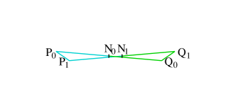
Figure 25: Darboux butterfly

Usually $P_{0},P_{1},Q_{0}$ are given and $Q_{1}$ is constructed. Compare this figure with fig. 7.

Consider a polygonal line $P_{0},P_{1},P_{2},...P_{n}$ with constant side length $P_{i}P_{i+1}=s$. Then one connects $P_{0}$ with $Q_{0}=P_{n}$ by the line $P_{0}Q_{0}=2d$. Then a point $P_{n+1}=Q_{1}$ is determined so that $Q_{0}Q_{1}=s,\quad P_{1}Q_{1}=P_{0}Q_{0}=2d$. $Q_{1}$ is the point which lies on the parallel to $P_{1}P_{n}$ through $P_{0}$. The arcs $P_{0}P_{1}$ and $Q_{0}Q_{1}$ in fig. 7 are equal. They are replaced by straight lines of equal length in the Darboux butterfly fig.25. In the limit considered here, where $P_{0}P_{1}=s$ tends to zero, the ratio of arc and distance tends to one. He argues that then Theorem I is equivalent to Theorem II and that this remains true when $s$ tends to 0 (and correspondingly $n$ to $\infty$). He restricts the corresponding curve $c$ to a curve without turning point. He considers the isosceles trapezoid $P_{i}P_{i+1}Q_{i}Q_{i+1}$ with circumcircles with centers $M_{i}$. This center is intersection point of the middle normals on $P_{i}P_{i+1}$, $Q_{i}Q_{i+1}$, but also on $P_{i}Q_{i}$, $P_{i+1}Q_{i+1}$. Denote the midpoint of $P_{i}Q_{i}$ by $N_{i}$ and that of $P_{i+1}Q_{i+1}$ by $N_{i+1}$. In the limit $s\rightarrow 0$ the points $N_{i}$ yield the curve $(N)$. The point $M_{i}$ yield the evolute $(M)$ of $(N)$. (I think, here is a misprint in the paper: Instead of ”die Punkte $N$ liegen auf einer Evolute der Kurve” it should read ”die Punkte $M$ liegen auf einer Evolute der Kurve”. A little bit later seems to be another misprint: Instead of ”Mittelpunkt der Sehne $PN$” one should read ”Mittelpunkte $N$ der Sehne $PQ$”.)

Salkowski continues: It may happen that the trapezoid degenerates to a rectangle. In this case the curve $(N)$ has a cusp. The tangents to the oval at the end points $P$ and $Q$ are parallel and perpendicular to $PQ$. If the arc $PQ$ is less than half of the circumference of the total circumference, then there exists an arc $P^{\prime}Q^{\prime}$ of the same length with $P^{\prime}Q^{\prime}$ parallel $PQ$, but shorter chord $P^{\prime}Q^{\prime}<PQ$. Thus the cusp of $(N)$ is only possible, if $PQ$ bisects the circumference. Such an example for $(N)$ is Steiner’s hypocycloid with three cusps.

He shows now
Theorem III. If a plane regular piece of curve has the property that three sets of chords of constant length $2d_{1},2d_{2},2d_{3}$ cut off constant lengths of curve and form a triangle, then the curve is a circle.
(Gericke[20] gave in 1936 another proof of this theorem).
Theorem IV. If all chords over constant arcs of length $2s$ of a curve have the same length $2d$ and the chords over arcs of length $s$ have the same length $2d^{\prime}$, then the curve is a circle.
Theorem IV’. If a set of quadrangles $PQRS$ with constant side lengths $2d_{1},2d_{2}$, $2d_{3},2d_{4}$ can be inscribed in an oval with corresponding constant arcs of curve, then the oval is a circle. In particular one finds
Theorem V. If all chords of an oval, which cut off one fourth of the circumference, have the same length, then the curve is a circle.

Finally Salkowski asks the general question: Are there ovals $c$, in which an $n$-gon with equal edges $2d$ can be shifted so that the corner points divide the perimeter in equal parts? One realizes that the area of the $n$-gon has to have constant size, further at least one angle is larger than a right angle. Consider three consecutive corners $P,Q,R$ of the figure with an obtuse angle at $Q$. Shift the chord $PQ$ continuously to $QR$, then the midpoint $N$ describes a piece of an oval $(N)$ and its evolute describes the curve $(M)$ of the midpoints of the circles, which touch the oval in the end points of the chords. Denote the midpoint of $PQ$ by $N_{0}$, the midpoint of $QR$ by $N_{1}$. $M_{0}$, $M_{1}$ are the intersections of the mid-normals on $PQ$ and $QR$, resp. $M$ is the intersection of the two mid-normals. Then the points $M_{0},M,M_{1}$ constitute a triangle with obtuse angle at $M$. The curve $(M)$ touches the mid-normals at $M_{0}$ and $M_{1}$.

So far I agree with the construction. But now Salkowski continues: Thus the piece of curve $MM_{0}$ (to my opinion it should read curve $M_{1}M_{0}$, since $M$ is generally not in the curve) is longer than the chord $M_{0}M_{1}$, thus larger than the distance $MM_{0}$. Since $M$ is the midpoint of the circumcircle of the isosceles triangle $PQR$, thus $MN_{0}=MN_{1}$, such a configuration is not possible unless $M,M_{0},M_{1}$ coincide. Then the triangle $PQR$ transforms into its neighboring position by an infinitesimal rotation, thus it remains unchanged during the shift along the curve $c$, hence remaining a circle.

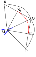
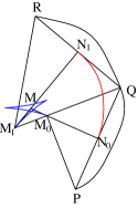
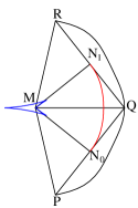
Figure 26: The construction by Salkowski

The curves $(P)$ are in black, $(N)$ in red, and $(M)$ in blue for $s_{Q}=\pi/7$, $\pi/14$, and $0$.

I do not see a reason, why $M,M_{0},M_{1}$ coincide in general. They will coincide at points where the curvature of $(P)$ at $Q$ has an extreme. Then the neighboring position need not be obtained by a mere rotation, since the distance $PR$ is not constant.

Salkowski has based his argument on an obtuse angle at $\angle PQR$. Such obtuse angles appear in several cases considered in ref. [58]. The curves (28) are convex for values $\epsilon$ up to approximately $1/(2p^{2})$. I choose the curve with $p=7$ fold symmetry and $\delta_{0}=52.959^{0}$, that is $\theta_{0}=37.041^{0}$. With $\epsilon=1/98$ the angle $\angle PQR$ varies between $102.99^{0}$ and $108.85^{0}$ and thus is always obtuse. I use an approximation in linear order in $\epsilon$ for the curve (P),

$$r(\phi)=1+2\epsilon\cos(p\phi),\quad\phi=s-\frac{\epsilon}{p}\sin(ps)$$ (123)

and choose

$$s_{P}=s_{Q}-2\theta_{0},\quad s_{R}=s_{Q}+2\theta_{0}.$$ (124)

The corresponding curves are shown in figure 26 for $s_{Q}=\pi/7$, $\pi/14$, and $0$. The curves $(P)$ are in black, $(N)$ in red, and $(M)$ in blue.

For $s_{Q}=0$ and $s_{Q}=\pi/7$ the three points $M$, $M_{0}$, and $M_{1}$ coincide. But in between, in particular for $s_{Q}=1/14$ the three points $M_{0}$, $M_{1}$, and $M$ differ. Note that curve $(M)$ has cusps. Thus the proof of his last theorem fails. This does not mean that his theorem is disproved. Since in terms of eqs. (123) the range for $\epsilon$ for convex boundaries becomes smaller with increasing $p$, it may be that there are not such ovals.

4.3.2 Auerbach 1938

Zindler had derived curves whose chords, which bisect the perimeter, have constant length and bisect the area. Auerbach[2] 1938 rederived the solution by Zindler, but he showed that these curves had also the property, that any chord acting as water-line yields the same potential energy, and thus all orientations are in equilibrium. The first five sections are for general densities $\rho$. He obtains for the curvatures at $P$ and $Q$

$$\kappa_{Q}-\kappa_{P}=2\frac{{\rm d}\theta}{{\rm d}s},\quad\kappa_{Q}+\kappa_{P}=\frac{4}{d}\sin\theta,$$ (125)

where $d/2$ is our $l$ and $\theta$ the angle between chord and tangent. From section 6 on he considers the case $\rho=1/2$. Auerbach derives the expressions for the coordinates $x,y$ of the boundary, eqs. (25, 26). One has to replace $(d/2)\rm{ctg}(\theta)\rightarrow\hat{\rho}$ and $d/2\rightarrow l$.

4.3.3 Ruban, Zalgaller, Kostelianetz 1939

Eugene Gutkin gives a few remarks of personal and socio-historical character at the end of his paper[26]. He reports the cruel death of Herman Auerbach under the Nazi regime. He also reports that the archimedean floating problem was popular among older mathematics students around 1939 in Leningrad. The results of three of them, Ruban, Zalgaller and Kostelianetz were published in the Proceedings (Doklady) of the Soviet Academy of Sciences in a Russian and a shorter French version.[43, 45] Only one of the authors, Zalgaller (often written Salgaller), could continue his career after the war. Kostelianetz did not return from the war. Ruban returned as invalid from the war, no longer able to do mathematics.

Although Ruban[43] and Salgaller and Kostelianetz[45] published side by side, they obtained contradictory results. Salgaller and Kostelianetz obtained solutions for $\rho=1/2$ in agreement with Zindler, but Ruban claimed that there are none besides the circle. Ruban obtained the second equation (125) and correctly found that $sin\theta$ of the angle $\theta$ between chord and tangent are equal at both ends of the tangent. Erroneously he concluded that both angles are equal, but they add up to $\pi$.

In sect. 5 of his paper[43] Ruban introduces the angle $\theta_{0}$ between chord and tangent and curvature $\kappa_{0}$ (Ruban uses $k$ instead of $\kappa$) of a circle of length $S$ and claims without proof or explanation: If

$$\theta_{0}{\rm ctg}\theta_{0}\not=\frac{\pi nl}{S}{\rm ctg}\frac{\pi nl}{S}$$ (126)

for $n=1,2,...$, then there exists a number $\epsilon>0$ so that the inequality $|\kappa(s)-\kappa_{0}|<\epsilon$ yields the equality $\kappa(s)=\kappa_{0}$, where $l$ is the length of the arc. Since $\theta_{0}=\pi l/S$, the inequality may be rewritten $C_{n}\not=0$ with

$$C_{n}=\cos(\theta_{0})\sin(n\theta_{0})-n\cos(n\theta_{0})\sin\theta_{0}.$$ (127)

It is likely that Ruban, who has derived the relation

$$b[\kappa(s+l)+\kappa(s)]=4\sin\theta(s)$$ (128)

in eq. (5) ($s$ is the arc parameter) and used a Fourier expansion for $\kappa(s)$ considered

$$\kappa(s)=\kappa_{0}+a_{n}\cos\frac{2\pi ns}{S}+b_{n}\sin\frac{2\pi ns}{S}.$$ (129)

Together with $2\theta(s)=\int_{s}^{s+l}{\rm d}t\kappa(t)$ and restricting to $a_{n}$ and $b_{n}$ in linear order yields condition $C_{n}=0$ for nontrivial solutions $a_{n}$, $b_{n}$. This is the starting point for non-circular perturbative solutions, as given in [58], where $\theta_{0}=\pi/2-\delta_{0}$. Thus Ruban was close to a solution, if he would have performed a perturbation expansion. Obviously $C_{n}=0$ is always fulfilled for $n=1$. It corresponds to a translation of the curve, compare sect. 4.2 of [58]. Thus Ruban’s statement should not include the case $n=1$.

In 1940 Geppert[19] gave the solutions for $\rho=1/2$, but erroneously argued that there are no solutions for $\rho\not=1/2$. He simply overlooked that in this later case the points on the boundary are end-points of two different chords, not one.

A general obstacle to find solutions for $\rho\not=1/2$ was that one expected that the circumference should be divided in an integer or at least rational number $n$ of equal parts. This was very good for $n=2$, $\rho=1/2$, but it is not at all necessary for $\rho\not=1/2$.

5 Algebraic Curves by Greenhill

In his 1899 paper[24] Greenhill gives special solutions expressed by pseudo-elliptic functions, in which the cosine and sine of the angle $n\theta$ and $n\theta/2$, resp. are algebraic functions of the radius $r$. Thus the curves are algebraic.

I do not attempt to go through the theory of the pseudo-elliptic functions, but refer only to the main results.

Starting point is the expression for the polar angle $\theta$ as function of the radius $r$,

$$\theta=\frac{1}{2}\int{\rm d}r^{2}\frac{Ar^{4}+Br^{2}+C}{r^{2}\sqrt{R}},\quad R=r^{2}-(Ar^{4}+Br^{2}+C)^{2}.$$ (130)

The integral is divided into two contributions,

$$\theta=\theta^{\prime}+(B-B^{\prime})u,$$ (131)

with

$$\theta^{\prime}=\frac{1}{2}\int{\rm d}r^{2}\frac{Ar^{4}+B^{\prime}r^{2}+C}{r^{2}\sqrt{R}},\quad u=\frac{1}{2}\int\frac{{\rm d}r^{2}}{\sqrt{R}},$$ (132)

where $u$ is the arc length.

The shape of the curves depends on two independent parameters. These may be the dimensionless $AC^{3}$ and $BC$, or $\epsilon$ and $\mu$ in [61], or $x$ and $y$ or $\beta$ and $\gamma$ by Greenhill.[24]

For a given periodicity in $\theta^{\prime}$, that is by an increase of $\theta^{\prime}$ by $2\pi/n$ (class I) or by $4\pi/n$, $n$ odd (class II), a certain relation between these parameters is fixed. Since at Greenhill’s time the integral for the arc length $u$, expressed as elliptic function of the first kind, was tabulated, one could easily calculate $\theta$ for these cases.

If moreover one requires $B=B^{\prime}$, in order to obtain an algebraic curve, one has a second condition, which allows only for single solutions.

5.1 Class I

For class I one finds solutions of the form

$$\sin(n\theta^{\prime}) = \frac{H(q)\sqrt{P_{1}}}{Qq^{n/2}},$$ (133)

$$\cos(n\theta^{\prime}) = \frac{L(q)\sqrt{P_{2}}}{Qq^{n/2}},$$ (134)

$$H(q) = q^{n-1}+h_{1}q^{n-2}+...+h_{n-1},$$ (135)

$$L(q) = q^{n-1}+l_{1}q^{n-2}+...+l_{n-1},$$ (136)

$$P_{1} = -q^{2}+2(2\gamma+1)q-1,$$ (137)

$$P_{2} = q^{2}+2(2\beta-2\gamma-1)q+(2\beta-1)^{2},$$ (138)

$$P = P_{1}P_{2}=-(q^{2}+2(\beta-2\gamma-1)q-2\beta+1)^{2}+16\beta^{2}\gamma q.$$ (139)

For $\gamma>0$ one uses $q=r^{2}$ and for $\gamma<-1$ one takes $q=-r^{2}$. $P$ is related to $R$ by

$$P=16\beta^{2}|\gamma|R=16\beta^{2}\gamma r^{2}-\left[4\beta\sqrt{|\gamma|}(Aq^{2}\pm Bq+C)\right]^{2}.$$ (140)

Hence $A,B,C$ are related to $\beta$ and $\gamma$ by

$$4\beta\sqrt{|\gamma|}=A,\quad\pm 8\beta\sqrt{|\gamma|}(\beta-2\gamma-1)=B,\quad 4\beta\sqrt{|\gamma|}(1-2\beta)=C.$$ (141)

The zeroes $q_{1,2}$ of $P_{1}$ are obtained as

$$q_{1,2}=2\gamma+1\pm 2\sqrt{\gamma(\gamma+1)}.$$ (142)

This yields the extreme values $r_{1,2}$ of $r$,

$$r_{1,2}=\left\{\begin{array}[]{cc}\sqrt{\gamma+1}\pm\sqrt{\gamma}&\gamma>0,\\ \sqrt{-\gamma}\pm\sqrt{-\gamma-1}&\gamma<-1.\end{array}\right.$$ (143)

The scale of $q$ is chosen so that $q_{1}q_{2}=1$. The other extreme values $q_{3,4}$ are the zeroes of $P_{2}$,

$$q_{3,4}=-2\beta+2\gamma+1\pm 2\sqrt{\gamma(2\beta-\gamma-1)}.$$ (144)

One may exchange $P_{1}$ and $P_{2}$ by simultaneously rescaling $q$. This yields

$$P_{1}(\beta,\gamma,q) = -(1-2\beta)^{2}P_{2}(\beta^{\prime},\gamma^{\prime},q^{\prime}),$$ (145)

$$P_{2}(\beta,\gamma,q) = -(1-2\beta)^{2}P_{1}(\beta^{\prime},\gamma^{\prime},q^{\prime}),$$ (146)

$$P(\beta,\gamma,q) = (1-2\beta)^{4}P(\beta^{\prime},\gamma^{\prime},q^{\prime}),$$ (147)

$$H(\beta,\gamma,q) = -(1-2\beta)^{n-1}L(\beta^{\prime},\gamma^{\prime},q^{\prime}),$$ (148)

$$L(\beta,\gamma,q) = -(1-2\beta)^{n-1}H(\beta^{\prime},\gamma^{\prime},q^{\prime})$$ (149)

with

$$\beta^{\prime}=\frac{-\beta}{1-2\beta},\quad\gamma^{\prime}=\frac{\gamma}{1-2\beta},\quad q^{\prime}=\frac{q}{1-2\beta}.$$ (150)

The derivative of $\theta^{\prime}$ calculated from eqs. (133, 134) yields

$$n\frac{{\rm d}\theta^{\prime}}{{\rm d}q} = \frac{2q\frac{{\rm d}H}{{\rm d}q}P_{1}+qH\frac{{\rm d}P_{1}}{{\rm d}q}-nHP_{1}}{2qL\sqrt{P_{1}P_{2}}}$$ (151)

$$= -\frac{2q\frac{{\rm d}L}{{\rm d}q}P_{2}+qL\frac{{\rm d}P_{2}}{{\rm d}q}-nLP_{2}}{2qH\sqrt{P_{1}P_{2}}}.$$ (152)

Thus one requires

$$2q\frac{{\rm d}H}{{\rm d}q}P_{1}+qH\frac{{\rm d}P_{1}}{{\rm d}q}-nHP_{1}=nLP^{\prime},$$ (153)

$$2q\frac{{\rm d}L}{{\rm d}q}P_{2}+qL\frac{{\rm d}P_{2}}{{\rm d}q}-nLP_{2}=-nHP^{\prime},$$ (154)

$$P^{\prime}:=q^{2}+2(\beta-2\gamma^{\prime}-1)q-2\beta+1,$$ (155)

so that

$$\frac{{\rm d}\theta^{\prime}}{{\rm d}q} = \frac{P^{\prime}}{2q\sqrt{P}}=\frac{R^{\prime}}{2q\sqrt{R}},$$ (156)

$$P^{\prime}=4\beta\sqrt{|\gamma|}R^{\prime} = Ar^{4}+B^{\prime}r^{2}+C,$$ (157)

$$B-B^{\prime} = \pm 16\beta\sqrt{|\gamma|}(\gamma^{\prime}-\gamma).$$ (158)

If one multiplies eq. (133) by $H$ and eq. (134) by $L$, and adds both equations, then one obtains

$$q^{n+1}\frac{{\rm d}}{{\rm d}q}\frac{H^{2}P_{1}+L^{2}P_{2}}{q^{n}}=0,$$ (159)

which yields after integration

$$\frac{H^{2}P_{1}+L^{2}P_{2}}{q^{n}}={\rm const.}$$ (160)

Denoting this constant by $Q^{2}$, one obtains

$$\cos^{2}(n\theta^{\prime})+\sin^{2}(n\theta^{\prime})=1,$$ (161)

as required.

From eqs. (133,134) one obtains

$$\cos(2n\theta^{\prime})=\frac{L^{2}(q)P_{2}-H^{2}(q)P_{1}}{Q^{2}q^{n}}.$$ (162)

Since

$$q^{n}\cos(2n\theta^{\prime})=\Re((x+{\rm i}y)^{2n})$$ (163)

and $q=x^{2}+y^{2}$, these curves are algebraic curves.

To obtain solutions for eqs. (133, 134) one has to solve eqs. (153-155). The coefficients $\beta$ and $\gamma$ are solutions of algebraic equations with integer coefficients.

$n$	$\beta$	$\gamma$	§ and fig. in [24]	fig. this paper
2	-1.36602540	-1.57735027	23 8	28
3	-0.37948166	-1.14356483	24 9	28
4	-0.19053133	-1.06944356	26 10	30
4	4.19179270	1.34344652	- -	30
5	-0.11633101	-1.04168414	27 11	32
5	-4.26375725	-2.97763686	- -	32
6	-0.07884381	-1.02799337	- -	34
6	2.21204454	0.41789155	- -	34

Table 1: Constants of curves class I

Figure 27: Curve with $n=2$

Figure 28: Curve with $n=3$

Figure 29: Curve with $n=4$

Figure 30: Curve with $n=4$

Figure 31: Curve with $n=5$

Figure 32: Curve with $n=5$

Figure 33: Curve with $n=6$

Figure 34: Curve with $n=6$

Several curves of class I are shown in figures 28 – 34. They are listed in table 1.

5.2 Class II

For class II the angle $\theta^{\prime}$ can be written for special values $A,B,C$ and odd $n$

$$\sin(\frac{n}{2}\theta^{\prime}) = \frac{H_{+}\sqrt{R_{+}}}{Qr^{n/2}},$$ (164)

$$\cos(\frac{n}{2}\theta^{\prime}) = \frac{H_{-}\sqrt{R_{-}}}{Qr^{n/2}},$$ (165)

$$H_{\pm} = r^{n-2}\pm h_{1}r^{n-3}+h_{2}r^{n-4}\pm...\pm h_{n-2},$$ (166)

$$R_{\pm} = r\pm(Ar^{4}+Br^{2}+C),$$ (167)

$$R = R_{+}R_{-}.$$ (168)

Differentiating (164, 165) one obtains

$$\frac{n{\rm d}\theta^{\prime}}{2{\rm d}r}=\pm\frac{2r\frac{{\rm d}H_{\pm}}{{\rm d}r}R_{\pm}+H_{\pm}r\frac{{\rm d}R_{\pm}}{{\rm d}r}-nH_{\pm}R_{\pm}}{2rH_{\mp}\sqrt{R_{-}R_{+}}}$$ (169)

This expression should yield

$$\frac{{\rm d}\theta^{\prime}}{{\rm d}r}=\frac{A^{\prime}r^{4}+B^{\prime}r^{2}+C^{\prime}}{r\sqrt{R}}$$ (170)

This requires

$$2r\frac{{\rm d}H_{\pm}}{{\rm d}r}R_{\pm}+H_{\pm}r\frac{{\rm d}R_{\pm}}{{\rm d}r}-nH_{\pm}R_{\pm}=\pm nH_{\mp}(A^{\prime}r^{4}+B^{\prime}r^{2}+C^{\prime}).$$ (171)

If we multiply the equation with the upper signs by $H_{+}$ and that with the lower signs by $H_{-}$, and add both then we obtain

$$r^{n+1}\frac{{\rm d}}{{\rm d}r}\frac{H_{+}^{2}R_{+}+H_{-}^{2}R_{-}}{r^{n}}=0,$$ (172)

which after integration yields

$$\frac{H_{+}^{2}R_{+}+H_{-}^{2}R_{-}}{r^{n}}={\rm const.}$$ (173)

which we set to $Q^{2}$. If we set

$$H_{1}=r^{n-2}+h_{2}r^{n-4}+...,\quad H_{2}=h_{1}r^{n-3}+h_{3}r^{n-5}+...,\quad P=Ar^{4}+Br^{2}+C,$$ (174)

so that

$$H_{\pm}=H_{1}\pm H_{2},\quad R_{\pm}=r\pm P,$$ (175)

then

$$H_{+}^{2}R_{+}+H_{-}^{2}R_{-}=2(H_{1}^{2}+H_{2}^{2})r+4H_{1}H_{2}P,$$ (176)

which is a polynomial of order $2n-1$ containing only terms with odd powers of $r$. Thus eq. (173) can only be fulfilled for odd $n$.

From eqs. (164, 165) one obtains

$$\cos(n\theta^{\prime})=\frac{H_{-}^{2}R_{-}-H_{+}^{2}R_{+}}{Q^{2}r^{n}}.$$ (177)

Since

$$r^{n}\cos(n\theta^{\prime})=\Re((x+{\rm i}y)^{n})$$ (178)

and

$$H_{-}^{2}R_{-}-H_{+}^{2}R_{+}=-2(H_{1}^{2}+H_{2}^{2})P-4H_{1}H_{2}r$$ (179)

is a polynomial even in $r$, these curves are algebraic, too.

Eq. (171) is an equation for a polynomial of order $n+2$ in $r$. Equating the coefficients of the powers $n+2$ and $n+1$ yields $nA=nA^{\prime}$ and $(n-2)Ah_{1}=-nA^{\prime}h_{1}$. $A=0$ would yield a constant curvature of the curve, thus only a circle or straight line, we require $A\not=0$. Hence $A^{\prime}=A$, $h_{1}=0$. The coefficients of the zeroth power in $r$ yield $-nCh_{n-2}=-nC^{\prime}h_{n-2}$. Thus if $h_{n-2}\not=0$, then $C^{\prime}=C$.

The simplest case is given by $n=3$. For this case one obtains $A^{\prime}=A$, $B^{\prime}=B/3$, $C^{\prime}=-C/3$. Here one does not obtain necessarily $C^{\prime}=C$, since $h_{1}=0$. Requiring $B^{\prime}=B$, $C^{\prime}=C$ yields

$$\sin(3\theta/2)=\frac{r\sqrt{r+Ar^{4}}}{\sqrt{2r^{3}}}=\sqrt{\frac{1+Ar^{3}}{2}},$$ (180)

$$\cos(3\theta/2)=\frac{r\sqrt{r-Ar^{4}}}{\sqrt{2r^{3}}}=\sqrt{\frac{1-Ar^{3}}{2}}.$$ (181)

Hence we obtain

$$\cos(3\theta)=-Ar^{3}$$ (182)

and with $A=-1/a^{3}$

$$r^{3}=a^{3}\cos(3\theta).$$ (183)

This curve is shown in figure 6.

For $n=5$ we find

$$B=\frac{1}{4C}-4AC^{2},\quad q=\sqrt{8}C$$ (184)

and

$$B^{\prime}=-\frac{1}{20C}-\frac{12AC^{2}}{5}.$$ (185)

Thus $B=B^{\prime}$ is obtained for

$$AC^{3}=\frac{3}{16},\quad BC=-\frac{1}{2}.$$ (186)

A remark on $n=5$ of Greenhill[24]. §14: The ratio of minimal radius and maximal radius is $(\sqrt[3]{10}-1)/3=0.38481156$ as given in the paper. §17 contains numerical errors: $c=(\sqrt[3]{10}-1)^{2}/3=0.44423982$, and the ratio of maximal radius and minmal radius is $(1+c)/(1-c)=2.59867451$, the inverse of the ratio of minimal and maximal radius in §14. The curves of §14 and §17 are not only of the same character, but they are the identical.

Figure 35: Curve with n=5

Figure 36: Curve with n=7

Figure 37: Curve with n=7

Figure 38: Curve with n=9

$n$	§and fig. in ref. [24]	fig. this paper
3	13 -	6
5	14 3	38
7	15 4	38
7	15 4	38
9	16 5	38

Table 2: Constants of curves class II

If we follow the curve with a continuous change of the direction of its tangent, then we have to circle twice around the origin in the figures 38, 38, 38, until we return to the start of the curve, whereas in figure 38 we have to do this only once. The curves are listed in table 2.

6 Bicycle Curves

Most of the elastica with and without pressure and the Zindler curves are bicycle curves. Finn[17] pointed out, that the class of bicycle curves is probably much larger. We will first comment on his ideas, but also on an important observation by Varkonyi[56] before we give some generalizations due to Mampel[40] and some closed curves with winding numbers different from one.

6.1 Circle of centroids

Tabachnikov[50] and also Salkowski[46] argue that one can give a segment of the front tire track. One draws the tangent at one point of the track of the back wheel in both directions and gives a smooth but arbitrary track of the front wheel between these two points. Then one can continue the tracks in both directions as for example described by Salkowski. Finn[17] instead starts with a segment of the back tire track, which is so long that the corresponding pieces of the front tire tracks meet themselves. In both cases certain conditions at the ends of the segments have to be met.

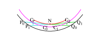
Figure 39: Bicycle tire tracks: Front track in black, rear track in red. Centroids of the areas enclosed by the cyan-green chords and the black track lie on the magenta circle

In section 2 and also section 6 of ref. [56] Varkonyi considered closed bicycle tracks. In fig. 39 two nearby locations of the bicycle moving to the left is shown in cyan and those of the bicycle moving to the right in green. They represent chords of length $2l$ of the black front track curve. These chords and the black line enclose areas ${\cal A}_{0}$ and ${\cal A}_{1}$ of constant size $A_{1}$. Their centroids are the points $C_{0}$ and $C_{1}$. Going from $P_{0}Q_{0}$ to $P_{1}Q_{1}$ the area $P_{0}P_{1}N$ is cut away and $Q_{0}Q_{1}N$ is added. These areas are $l^{2}\alpha/2$ with (infinitesimal) angle $\alpha$ between the two chords. Their centroids $C_{P}$ and $C_{Q}$ are $2l/3$ apart from the point of intersection $N$ of the two chords. Thus the centroid moves from $C_{0}$ to $C_{1}$ by the distance $r\alpha$ with $r_{1}=2l^{3}/(3A_{1})$ parallel to the chords. Since $l$ and $A_{1}$ are constant, the centroids lie on a circle of radius $r_{1}$.

Varkonyi now argues: If the bicycle curve is closed, then the same arguments apply for the complementary area of size $A_{2}=A-A_{1}$, where $A$ is the area enclosed by the black front track. The centroids of the complementary area lie on a circle of radius $r_{2}=2l^{3}/(3A_{2})$. In general it is not clear, whether these two circles are concentric. Thus it is not clear whether closed bicycle curves correspond to the boundaries of homogeneous floating bodies of equilibrium. The centroid of the whole area lies on the connecting line between the centers of the two circles. If one allows for an inhomogeneus body, then the volume centroid and the mass centroid can differ. Then one obtains floating bodies of equilibrium, if the mass centroid lies in one of the circle centers. For density $\rho=1/2$ both circles are identical. The known boundaries for $\rho\not=1/2$. have dieder symmetry. Thus also the centers of the circles are concentric. Whether there are other solutions for closed bicycle tracks is not known.

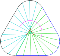
Figure 40: Nearly a triangle with rounded corners

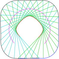
Figure 41: Nearly a square with rounded corners

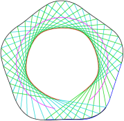
Figure 42: Nearly a pentagon with rounded corners

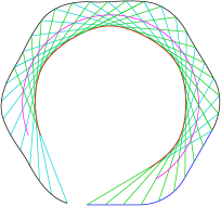
Figure 43: Nearly a hexagon with rounded corners

We give several examples of bicycle curves in the following. The segment of the front tire track from which we start is shown in blue. The following tire track is determined by adding Darboux butterflies and shown in black. (For Darboux butterflies see subsection 4.3.1 and figure 25). Chords are drawn after every fifth application of the butterfly. The centroids of the enclosed area are connected and shown in magenta. The appearence resembles part of a circle. In figures 41 to 43 the initial segment consists of three pieces, first a straight line of length $s/3$, then a circular arc of the same length $s/3$ and then again a straight line of length $s/3$. The circular arc changes the direction by an angle $2\pi/n$ with $n=3,4,5,6$ for figs. 41, 41, 43, and 43, respectively. The front tracks close nearly and show approximately polygons with $n$ rounded corners. The butterfly procedure generates nearly circular arcs from the (nearly) straight lines and nearly straight lines from the arcs. These curves are very similar to the figures 9 and 11, the first and third of fig. 13, the first of fig. 14, and fig. 52.

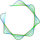
Figure 44: Based on eq. (187) with $c=2$

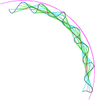
Figure 45: Based on eq. (187) with $c=4$

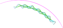
Figure 46: Based on eq. (187) with $c=4.5$

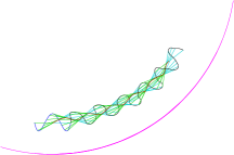
Figure 47: Based on eq. (187) with $c=5.5$

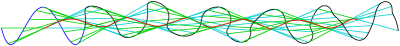
Figure 48: Based on eq. (187) with $c=5$

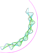
Figure 49: Based on eq. (187) with $c=6$

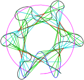
Figure 50: Based on eq. (187) with $c=8$

A second class of front tire tracks are shown in figures 45 to 50. The initial front track segment is given by

$$y=b(1-x^{2})(1-cx^{2}).$$ (187)

We have chosen $b=1/2$ for all figures and $c=2,4,4.5,5.5,5,6,8$ for figures 45 to 50. The area on both sides of the chord are counted with opposite sign. Thus the ’centroid’ may lie outside the areas. For $c=5$ (fig. 48) the ares on both sides of the chord are equal. Thus a centroid is not defined in this case or lies at infinity. From fig. 50 we see that the tracks may become very wild. This is also the case, if we use larger values of $b$ in eq. (187).

6.2 Zindler multicurves

Of course the curves we found for the floating bodies of equilibrium had to be closed after one revolution. This is not required for bicycle curves. Also the Zindler curves can be generalized to a larger class of bicycle curves, which I call Zindler multicurves.

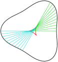
Figure 51: Zindler curve with $m=1,n=3$

Figure 52: Zindler curve with $m=1,n=5$

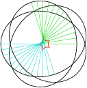
Figure 53: Zindler multicurve with $m=3,n=5$

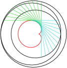
Figure 54: Zindler multicurve with $m=3,n=1$

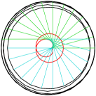
Figure 55: Zindler multicurve with $m=5,n=1$

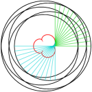
Figure 56: Zindler multicurve with $m=5,n=3$

The definition of the Zindler curves is generalized by replacing eqs. (25, 26) to

$$x(\alpha)=l\cos(m\alpha)+\xi(\alpha), y(\alpha)=l\sin(m\alpha)+\eta(\alpha),$$ (188)

$$\xi(\alpha)=\int^{\alpha}{\rm d}\beta\cos(m\beta)\hat{\rho}(\beta), \eta(\alpha)=\int^{\alpha}{\rm d}\beta\sin(m\beta)\hat{\rho}(\beta),$$ (189)

where $m$ is an odd integer. The radius of curvature is now $|\hat{\rho}/m|$. As in (27) we require

$$\xi(\alpha+\pi)=\xi(\alpha),\quad\eta(\alpha+\pi)=\eta(\alpha),$$ (190)

which again implies $\hat{\rho}(\beta+\pi)=-\hat{\rho}(\beta)$. The curves for $m=1$ are Zindler curves. For larger $m$ the curves are no longer double point free. Generally they repeat only after $m$ revolutions. These curves are also bicycle curves, since the argument around eq. (29) applies again.

Examples are

$$\hat{\rho}(\beta)=(m^{2}-n^{2})\sin(n\beta)$$ (191)

with odd $n$, $n\not=m$, and $n,m$ coprime. One obtains for the envelopes (traces of the rear wheels)

$$\xi(\alpha) = \frac{n-m}{2}\cos((n+m)\alpha)+\frac{n+m}{2}\cos((n-m)\alpha),$$ (192)

$$\eta(\alpha) = \frac{n-m}{2}\sin((n+m)\alpha)-\frac{n+m}{2}\sin((n-m)\alpha).$$ (193)

These envelopes are known as hypocycloids for $n>m$ and as epicycloids for $n<m$. They wind $m$ times around the origin and have $n$ cusps. These cusps point outward for hypocycloids and inward for epicycloids. With $\alpha=u/2$ the Zindler multicurve is parametrized by

$$z=x+{\rm i}y=\frac{n-m}{2}{\rm e}^{{\rm i}(n+m)u/2}+\frac{n+m}{2}{\rm e}^{{\rm i}(m-n)u/2}+l{\rm e}^{{\rm i}mu/2}.$$ (194)

In particular for $m=1,n=3$ one obtains

$$z={\rm e}^{2{\rm i}u}+2{\rm e}^{-{\rm i}u}+l{\rm e}^{{\rm i}u/2}.$$ (195)

Examples of such Zindler curves, $m=1$, are shown in figures 52 and 52. We show four examples of Zindler multicurves with $m=3$ and $m=5$ in figures 54 to 56.

6.3 Mampel’s generalized Zindler curves

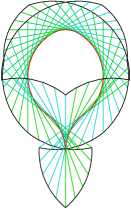
Figure 57: Envelope with one cusp pointing outside

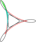
Figure 58: Curve according to (195) with $l=1.6$.

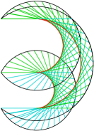
Figure 59: Three cusps pointing to the left.

Mampel[40] considers generalized Zindler curves. He introduces envelopes (denoted as ’Kern’ $\cal{K}$) with an odd number of cusps. He attaches tangents with constant length $l$ in both directions. The endpoints of the tangents form his generalized Zindler curves $\cal{Z}$, irrespective of any convexity. Examples similar to Mampel’s figures 8a, 8b, and 9, are shown in figures 59 to 59. The curves 59 and 59 consist of circular arcs. The envelope of fig. 59 is a hypocycloid.

6.4 Other bicycle curves

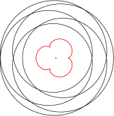
Figure 60: Curves with ratio = 1.72

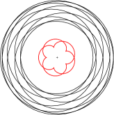
Figure 61: Curves with ratio = 1.582

We show some buckled rings, which turn around the center several times. The ratio of the maximal radius and the minimal radius is given. The buckled ring figure 61 is very similar to the Zindler multicurve figure 56.

Figures 61 to 67 show buckled rings which turn around the center nine times. These buckled rings have two different envelopes. The smaller one has five cusps pointing inward, figure 61. The outer envelope, figure 65 has no cusps. If the ratio of the largest distance to the smallest distance from the center is not too large, then the outer trace for the rear tire is without cusps. This is the case for the figures 63 to 65. If the ratio becomes larger, then cusps appear as seen in figures 65 to 67.

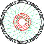
Figure 62: Curves with ratio = 1.1546

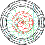
Figure 63: Curves with ratio = 1.399

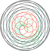
Figure 64: Curves with ratio = 1.582

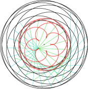
Figure 65: Curves with ratio = 1.8637

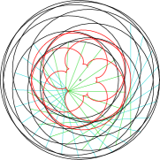
Figure 66: Curves with ratio = 2.0869

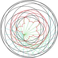
Figure 67: Curves with ratio = 2.4451

7 Conclusion

A short historical account of the curves related to the two-dimensional floating bodies of equilibrium and the bicycle problem is given in this paper. Bor, Levi, Perline and Tabachnikov found that quite a number of the boundary curves had already been described as Elastica and Elastica under Pressure or Buckled Rings. Auerbach already realized that curves described by Zindler are solutions for the floating bodies problem of density 1/2. An even larger class of curves solves the bicycle problem.

The subsequent sections deal with some supplemental details: Several derivations of the equations for the elastica and elastica under pressure are given. The properties of Zindler curves and some work on the problem of floating bodies of equilibrium by other mathematicians is discussed. Special cases of elastica under pressure lead to algebraic curves as shown by Greenhill. Since most of the curves considered here are bicycle curves, we added some remarks on them.

Acknowledgment I am indebted to Sergei Tabachnikov for many useful discussions. I am grateful to J.A. Hanna and M. Bialy for useful information.

References

- [1] G. Arreaga, R. Capovilla, C. Chryssomalakos, J. Guven, Area-constrained planar elastica, Phys. Rev. E 65 (2002) 031801
- [2] H. Auerbach, Sur une probl‘eme de M. Ulam concernant l’‘equilibre des corps flottants. Studia Math. 7 (1938) 121-142
- [3] R. Balarini, The Da Vinci-Euler-Bernoulli Beam Theory? Mechanical Engineering Magazine Online (April 18, 2003)
- [4] J. Bernoulli, Quadratura curvae, e cujus evolutione describtur inflexae laminae curvatura. In Die Werke von Jakob Bernoulli, Birkhäuser
- [5] J. Bernoulli, Jacobi Bernoulli, Basiliensis, Opera vol. 1 (1744) Cramer & Philibert, Geneva
- [6] M. Bialy, A.E. Mironov, L. Shalom, Magnetic billiards: Non-integrability for strong magnetic field; Gutkin type examples, arXiv: 2001.02119v1
- [7] G. Bor, M. Levi, R. Perline, S. Tabachnikov, Tire track geometry and integrable curve evolution, arxiv: 1705.06314
- [8] M. Born, Untersuchungen über die Stabilität der elastischen Linie in Ebene und Raum, unter verschiedenen Grenzbedingungen, PhD Thesis. Universität Göttingen (1906) https://archive.org/details/untersuchungenb00borngoog/page/n5
- [9] J. Bracho, L. Montejano, D. Oliveros, A classification theorem for Zindler Carousels, J. Dynam. Control Systems 7 (2001) 367
- [10] J. Bracho, L. Montejano, D. Oliveros, Zindler curves and the floating body problem, Period. Math. Hungar 49 (2004) 9
- [11] R. Capovilla, C. Chryssomalakos, J. Guven, Elastica hypoarealis, Eur. Phys. J. B 29 (2002) 163-166
- [12] Journal für die reine und angewandte Mathematik (Crelles Journal) vol. 1 (1826) – 4(1929)
- [13] A.C. Doyle, The Adventure of the Priory School in The Return of Sherlock Holmes, McClure, Philips & Co. (New York 1905), Georges Newnes, Ltd. (London 1905)
- [14] L. Euler, Additamentum: De curvis elasticis in Methodus inveniendi lineas curvas maximi minimive proprietate gaudentes, Lausanne (1744); Translated and annotated by W.A. Oldfather, C.A. Ellis, and D.M. Brown Leonhard Euler’s elastic curves Isis 20 (1933) 72-160, http://www.jstor.org/stable/224885; Übersetzt von H. Linsenbarth, in Abhandlungen über das Gleichgewicht und die Schwingungen der ebenen elastischen Kurven, Ostwald’s Klassiker der exakten Wissenschaften 175 (Leipzig 1910)
- [15] F. Evers, A.D. Mirlin, D.G. Polyakov, P. Wölfle, Semiclassical theory of transport in a random magnetic field, Phys. Rev. B60 (1999) 8951; cond-mat/9901070
- [16] R. Ferréol, Encyclopédie des formes mathématiques remarquables, www.mathcurve.com
- [17] D.L. Finn, Which way did you say that bicycle went? http://www.rose-hulman.edu/finn/research/bicycle/tracks.html
- [18] D.L. Finn, Which way did you say that bicycle went? Math. Mag. 77 (2004) 357-367
- [19] H. Geppert, Über einige Kennzeichnungen des Kreises, Math. Z. 46 (1940) 117-128
- [20] H. Gericke, Einige kennzeichnende Eigenschaften des Kreises, Math. Z. 40 (1936) 417
- [21] E.N. Gilbert, How Things Float, Am, Math. Monthly 98 (1991) 201
- [22] I. Goldin, J-M. Delosme, A.M. Bruckstein, Vesicles and Amoebae: On Globally Constrained Shape Deformation, J. Math. Imaging and Vision 37 (2010) 112
- [23] A.G. Greenhill, The applications of elliptic functions, MacMillan & Co, London, New York (1892)
- [24] A.G. Greenhill, The elastic curve, under uniform normal pressure, Mathematische Annalen LII (1899) 465
- [25] E. Gutkin, Capillary Floating and the Billiard Ball Problem, J. Math. Fluid Mech. 14 (2012) 363-382
- [26] E. Gutkin, Addendum to: Capillary Floating and the Billiard Ball Problem, J. Math. Fluid Mech. 15 (2013) 425
- [27] G.-H. Halphen, Sur une courbe elastique, Journal de l’ecole polytechnique, cahier (1884) p.183 (available via gallica.bnf.fr)
- [28] G.-H. Halphen, La courbe elastique plane sous pression uniforme, Chap. V in Traite des fonctions elliptiques et de leurs applications, Deuxieme partie. Applications a la mecanique, a la physique, a la geodesie, a la geometrie et au calcul integral. p. 192
- [29] W. Helfrich, Elastic Properties of Lipid Bilayers: Theory and Possible Experiments, Z. Naturforsch. 28c (1973) 693-703
- [30] J. Hirakawa, On a characteristic property of the circle, The Tôhoku Math. Journal 37 (1933) 175
- [31] C. Huygens, Constructio universalis problematis …, Acta Eruditorum Leipzig 1694 p. 338
- [32] C.G.J. Jacobi, Fundamenta nova theoriae functionum ellipticarum, Königsberg, Bornträger 1829
- [33] G. Kirchhoff, Über das Gleichgewicht und die Bewegung eines unendlich dünnen elastischen Stabes, J. reine u. angewandte Math. 56 (1859) 285-313
- [34] J. Langer, Recursion in Curve Geometry, New York J. of mathematics 5 (1999) 25-51
- [35] J. Langer, D.A. Singer, The total squared curvature of closed curves, J. Differential Geometry 20 (1984) 1-22
- [36] P. S. Laplace, Oeuvres complétes de Laplace, vol. 4, Gauthiers-Villars (1880)
- [37] R. Levien, The elastica: A mathematical history, www.levien.com/ phd/elastica_hist.pdf
- [38] M. Lévy, Memoire sur un nouveau cas integrable du probleme de l’elastique et l’une des ses applications, Journal de Mathematiques pures et appliquees serie, tome 10 (1884) p. 5-42
- [39] A.E.H. Love, A Treatise on the Mathematical Theory of Elasticity, Cambridge University Press (1927), p. 263
- [40] K.L. Mampel, Über Zindlerkurven Jour. für die reine und angewandte Mathematik 234 (1967) 12-44
- [41] D. Oliveros, L. Montejano, De volantines, espirógraphos y la flotación de los cuerpos, Revista Ciencias 55-56 (1999) 46-53
- [42] M. Rédei, On the tension between mathematics and physics, http://philsci-archive.pitt.edu/16071/ (2019)
- [43] A.N. Ruban, Sur le problème du cylindre flottant, Comptes Rendus (Doklady) de l’Académie des Sciences de l’URSS, XXV (1939) 350
- [44] L. Saalschütz, Der belastete Stab unter Einwirkung einer seitlichen Kraft, B.G. Teubner, Leipzig (1880)
- [45] V. Salgaller and P. Kostelianetz, Sur le problème du cylindre flottant, Comptes Rendus (Doklady) de l’Académie des Sciences de l’URSS, XXV (1939) 353
- [46] E. Salkowski, Eine kennzeichnende Eigenschaft des Kreises, Heinrich Liebmann zum 60. Geburtstag, Sitz.berichte der Heidelberger Akademie der Wissenschaften (1934) 57-62
- [47] D.A. Singer, Lectures on elastic curves and rods, Curvature and variational modeling in physics and biophysics, AIP Conference Proc. 1002 (2008) 3-32
- [48] H. Singh, J.A. Hanna, On the planar Elastica, Stress, and Material Stress, Jour. of Elasticity 136 (2019) 87-101
- [49] S. Svetina, B. Žekš, Membrane bending energy and shape determination of phospholipid vesicles and red blood cells, Eur. Biophysics J 17 (1989) 101-111
- [50] S. Tabachnikov, Tire track geometry: variations on a theme, Israel J. of Math. 151 (2006) 1-28 archive math.DG/0405445
- [51] I. Tadjbakhsh, F. Odeh, Equilibrium states of elastic rings, J. Math. Anal. Appl. 18 (1967) 59-74
- [52] I. Todhunter, (K. Pearson, ed.), A History of the Theory of Elasticity and of the Strength of Materials, 2 volumes, Cambridge University Press (1886, 1893). See also: en.wikiquote.org/wiki/A_History_of_ the_Theory_of_Elasticity_and_of_the_Strength_of_Materials
- [53] C. Truesdell, The rational mechanics of flexible or elastic bodies: 1638-1788, in: Leonhard Euler, Opera Omnia, Orell Füssli Turici, ser. 2, vol. XI, 2 (1960)
- [54] C. Truesdell, Der Briefwechsel von Jacob Bernoulli, chapter Mechanics, especially Elasticity, in the correspondence of Jacob Bernoulli with Leibniz. Birkhäusser (1987)
- [55] S. Ulam, Problem 19 in The Scottish Book, ed. R.D. Mauldin, Birkhäuser (2015)
- [56] P.L. Varkonyi, Floating Body Problems in Two Dimensions, Studies in Appl. Mathemetics 122 (2009) 195-218
- [57] F. Wegner, Floating Bodies of Equilibrium, Studies in Applied Mathematics 111 (2003) 167-183
- [58] F. Wegner, Floating bodies of equilibrium I, arxiv: Physics/0203061
- [59] F. Wegner, Floating bodies of equilibrium II, arxiv: Physics/0205059
- [60] F. Wegner Floating bodies of equilibrium. Explicit Solution, arxiv: Physics/0603160
- [61] F. Wegner, Floating bodies of equilibrium in 2D, the tire track problem and electrons in a parabolic magnetic field, arxiv: Physics/0701241v3
- [62] Wikipedia contributors, Euler-Bernoulli beam theory, Wikipedia, The Free Encyclopedia, https://en.wikipedia.org/wiki/Euler-Bernoulli_beam_theory
- [63] K. Zindler, Über konvexe Gebilde. II. Teil, Monatsh. Math. Physik 31 (1921) 25-57