Tutorial
Low-cost Wireless Condition Monitoring System for an Ultracold Atom Machine

Abstract

We present a flexible wireless monitoring system for condition-based maintenance and diagnostics tailored for dynamic and complex experimental setups encountered in modern research laboratories. Our platform leverages an Internet-of-Things approach to monitor a wide range of physical parameters via wireless sensor modules that broadcast to a networked computer. We give a specific demonstration for a so-called ultracold atom machine, which is the workhorse of many emerging quantum technologies and marries a broad spectrum of equipment and instrumentation into its setup. As a distinctive feature, our monitoring system taps into physical parameters of the ultracold atom machine both via customized sensor modules that directly perform measurements, and via modules that recruit and annex constituent instruments of the machine for the additional purpose of retrieving information for diagnostics.

1 Introduction

The advent of laser cooling opened up a way to produce trapped atomic gases at temperatures only a few microkelvin above absolute zero, initiating the field of ultracold atomic physics [1]. Augmenting laser cooling with evaporative cooling, a push was made to the nanokelvin domain where Bose-Einstein condensates and degenerate Fermi gases were attained. These ultracold atomic systems have remained at the cutting-edge of research because they offer a pristine environment to explore fundamental quantum phenomena, and the experimental platforms used in their production can accurately be referred to as ‘ultracold atom machines’ [2, 3]. Such machines—an example is shown in Fig. 1—are extremely complex, hybridising many different technologies from optical, microwave, vacuum, electronic, and mechanical engineering. They typically incorporate a range of both commercially available equipment and custom-built hardware, patching a variety of systems together to get a functional ultracold atom machine and an optimised process sequence. The end product of running a process cycle—a small gas cloud a few billionths of a degree above absolute zero temperature, levitated inside a vacuum chamber by electromagnetic fields—is extremely sensitive to changes in the process parameters and the environment. A reproducible result is hence strongly tied to these conditions remaining stable. Accordingly, detected variations in the end product such as atom number, quantum state purity or sample temperature may be associated with variations in specific, monitored process parameters through suitable analysis. For example, Ref. [4] employed commercial data acquisition hardware to monitor 50 parameters of an ultracold atom machine and tied fluctuations in the final atom number to the temperature of a magnetic field coil.

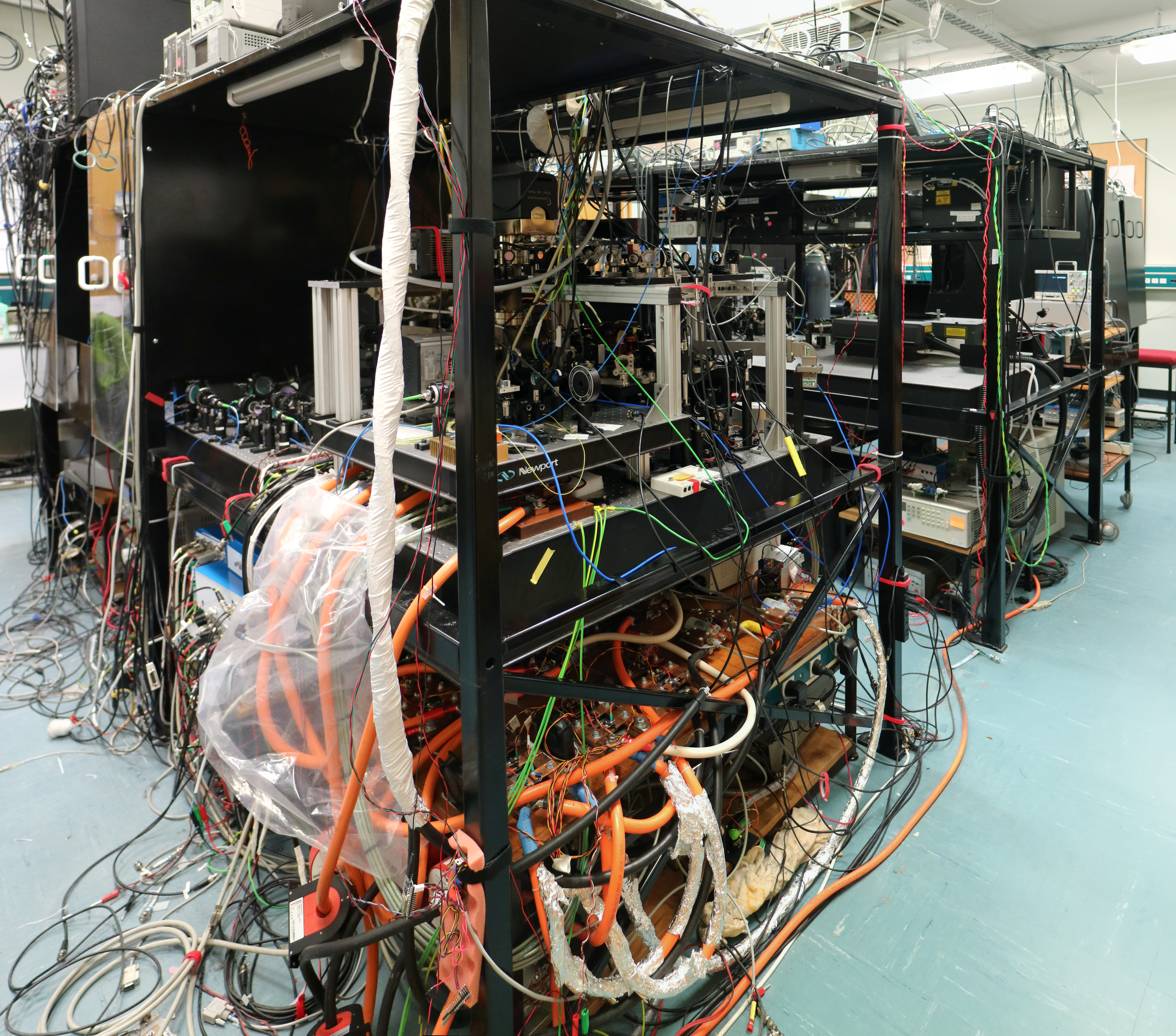
Fig. 1: The ultracold atom machine at the University of Otago. Equipment spans three $1.2\text{\times}3\text{\,}\mathrm{m}$ optical tables in four tiers. The experiment confines atoms inside an ultra-high vaccum chamber using high-current-carrying ($\sim 400$ A) magnetic field coils. The trapped atoms are manipulated by $\sim 10$ different laser systems, 3 different microwave and RF emitters, and $\sim 10$ auxiliary magnetic field coils. The machine is a hybrid of many different technologies from optical, microwave, vacuum, electronic, and mechanical engineering and incorporates a range of both commercially available equipment and custom-built hardware.

Condition monitoring [5] is a well known paradigm in conventional industrial plants, where monitoring equipment parameters allows for condition-based or predictive maintenance and leads to increased equipment up-time and smaller maintenance and operating costs. These benefits could also be reaped in a research laboratory setting, where, however, particular challenges emerge when dealing with commercial test and measurement equipment. Past generations of, for example, microwave frequency synthesizers, current supplies, and laser controllers will not natively interface with a condition monitoring system. Such equipment might however represent a considerable investment and from performance point of view remain completely adequate: a high-end Hewlett Packard 26 GHz YIG based synthesizer from the 1980s remains a fine instrument today. Incorporation of such instruments into a monitoring system along with a range of sensor modules can be achieved using ‘Internet-of-Things’ (IoT) technologies and ideas – an approach which is formed around having large numbers of devices (‘things’) connected to the Internet [6], and which has grown in popularity with the availability and declining cost of hardware with networking capability. IoT ideas are also finding use in home automation [7], wearable technology, healthcare [8, 9, 10], and are moving into wireless sensor network technologies in conventional processing plants [11, 12]. Wireless sensor networks themselves are used in numerous settings including sailboats [13], launch vehicles [14], heritage buildings [15], agriculture[16, 17], composting [18], and environmental [19, 20] and land slide monitoring [21, 22].

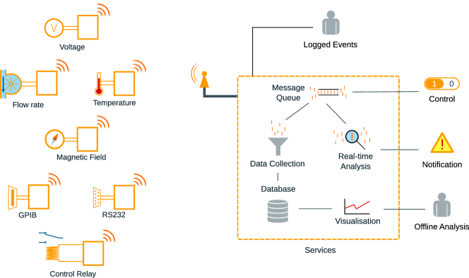
Fig. 2: The architecture and data-flow pipeline of the monitoring system. Some examples of the sensors we use are shown.

In this paper, we focus on a wireless, low-cost, long-term monitoring system, with an emphasis on experimental apparatus, which entails interfacing with both commercial laboratory equipment (for example via IEEE-488 or RS-232) and home-built, customized sensors using IEEE 802.11b/g/n WiFi as the communication backbone. Our monitoring system straddles these dual domains and augments a wireless sensor network with services for data collection and analysis as illustrated in Fig. 2. We have tested our monitoring system over a period of 2 years in connection to an ultracold atom machine at the University of Otago which over the past decade has developed into an apparatus of significant complexity [23, 24, 25, 26, 27, 28]. We have found the operation of the monitoring system robust, reliable, and useful in detecting equipment failures in our laboratory, especially those of a chiller used for cooling water, and the lab air conditioning – saving us from further equipment failure, and answering the questions “does it feel warm in here?” and “why is the experiment performing badly” with logged data. More recently, we have extended our data logging framework to contact tracing of lab users during the COVID19 pandemic. In the following we will describe key features of our monitoring system, including the construction of wireless sensor modules, examples of their usage and their integration into a flexible architecture that can log data from a diverse range of sources.

2 Sensor Module

Our sensor modules are based on either the ESP8266 or ESP32 micro-controllers by Espressif Systems which are self-contained System-on-Chips with built-in WiFi. These modules also contain analog-to-digital converters (ADCs), digital serial capabilities (including UART, I2C, SDIO, SPI), and a number of general-purpose input-output (GPIO) pins. We specifically use the NodeMCU V1.0 [31] and the DevKit C development boards for the ESP8266 and ESP32, respectively, which add USB serial interfaces for convenient programming as well as a supply voltage regulator.

Each of our sensor modules is programmed with firmware we have developed according to the application and containing drivers for the connected sensor. Table 1 shows the cost of the development boards, and the extra hardware for three typical example nodes—a simple temperature sensor, an RS-232 interface, and a wireless General Purpose Interface Bus (GPIB) module.

Our code [30] provides a ready-to-use framework where firmware is uploaded to the ESP development board via its USB connection (we use the PlatformIO tools [32] for this purpose). Once deployed, the device can be reprogrammed via WiFi from a web-browser. Our code library contains detailed information and instructions on configuring and deploying the modules. Essentially, the steps to be followed can be summarized as:

• Set up the data collection services on a networked computer in the laboratory (only needs to be done once).

• Connect sensors to the ESP development board.

• Specify the connected sensors in the code.

• Build firmware on computer (via PlatformIO) and upload it to the development board via USB (the sensor module will then broadcast a WiFi network to configure its connection).

• Deploy sensor module in lab.

• Connect to WiFi broadcast by the sensor module to connect to WiFi in the lab and publish measurements to the data collection server.

Below we present a range of the sensors that we have deployed in our laboratory and for which we provide code and hardware examples.

Table 1: Typical Bill of Materials for monitoring nodes.

Part	Price (USD)
Controller Development Boards
ESP32 DevKit C	$7.49
ESP8266 (NodeMCU V2)	$5.99
GPIB Monitor
GPIB Connector (e.g. DigiKey 1024RMA-ND)	$5.53
Arduino Nano	$4.66
$1\text{\,}\mathrm{k\SIUnitSymbolOhm}$ Resistor	$0.01
PCB Manufacture	$2.00
RS232 Monitor
DB9 Connector	$0.77
MAX202 Transceiver	$1.03
$1\text{\,}\mathrm{k\SIUnitSymbolOhm}$ Resistor	$0.01
$4\times$$100\text{\,}\mathrm{nF}$ Capacitors	$0.01
PCB Manufacture	$2.00
Temperature Monitor
DS18B20 Thermometer	$1.69

2.1 Temperature Sensor

For contact temperature measurement we primarily use the DS18B20 from Maxim Integrated, which we fit into various places in our machine. Each sensor has a digital interface, and is capable of reporting the temperature to a resolution as good as $62.5\text{\,}\mathrm{mK}$ [33]. We find the TO-92 package (small “transistor” shape) of the DS18B20 to be a convenient size to locate throughout our apparatus. We also employ variants enclosed in a water-proof housing.

To construct a wireless sensor module from the DS18B20, one can simply connect it to an ESP8266 as shown in Fig. 3(a), then configure the firmware specifying a DS18B20 is connected, and a handle to identify the measurement. Multiple DS18B20 devices can be connected to the same GPIO pin and read out separately as they have unique IDs.

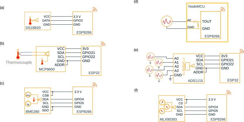
Fig. 3: Connection diagrams for wireless sensor modules for measuring contact temperature (a), (b), environmental temperature humidity and pressure (c), analog voltages (d), (e), and magnetic fields (f). The modules (b), (c), (e), and (f) integrate I2C sensors, which rely on power lines and two connections for the serial interface. Many of the sensors we use additionally require configuration by setting the voltage of another pin on the sensor, e.g. CS, CSB, SDO and ADDR above

For an even smaller sensor head or to measure temperatures exceeding $125\text{\,}\mathrm{\SIUnitSymbolCelsius}$, we use K-type thermocouples, with the MCP9600 16-bit thermocouple-to-digital converter from Microchip (see Fig. 3(b)). This device features all the required signal conditioning, supports multiple types of thermocouples, and has built-in compensation for the cold junction formed by physically connecting the thermocouple to the converter.

2.2 Atmospheric Sensors

To measure atmospheric signals of interest, such as ambient temperature and humidity, we use the AM2302 from Aosong Electronics – a small digital sensor which can measure the ambient temperature and relative humidity. Another sensor we use for this purpose is the BME280 from Bosch Sensortec, which additionally measures the atmospheric pressure (see Fig. 3(c)).

From these signals one can, for example, detect changes in the lab environmental control or the function of a positive pressure environment. In particular, we have found it useful to monitor the outside temperature with an atmospheric sensor module mounted on the side of the building to examine the impact of weather on our cooling water system’s performance. Monitoring the performance of the lab air conditioning has also proven useful.

2.3 Analog Voltage Measurements

Virtually any physical quantity we want to measure can be converted to an analog voltage by some electrical transducer, for example: currents (using a sense resistor, or hall-effect sensor), resistance (using a bridge circuit), temperatures (using a thermistor), forces/pressures (with a strain gauge), and magnetic fields (with hall-effect sensors). Furthermore, many industrial sensors produce an analog signal of 4–20 $\mathrm{mA}$, and many research instruments provide a voltage output to monitor signals of interest. The variety of applications for monitoring analog signals makes this an important requirement of our framework. Fig. 3 (d) and (e) shows two configurations for this task.

2.3.1 Internal ADC

The ESP8266 features an on-chip 10-bit ADC with a native $0\text{\,}\mathrm{V}1\text{\,}\mathrm{V}$ range, which on the NodeMCU boards has been extended to a $0\text{\,}\mathrm{V}3.2\text{\,}\mathrm{V}$ range with a 220:100 $\mathrm{k\SIUnitSymbolOhm}$ resistive voltage divider. This range can be adjusted by suitable replacement of the resistors of the NodeMCU board or by adding a resistor inline with the signal.

The ESP32 includes two 12-bit ADCs, which can be configured to take maximum voltages of up to $3.3\text{\,}\mathrm{V}$. These ADCs can be configured to measure on a number of different GPIO pins, meaning that one can monitor multiple signals in parallel. However, the ESP32’s ADCs suffer from non-linearity in their readings (see supplementary material), so we recommend using the ADS1115 external ADC, which we describe below.

The on-chip ADC is referenced to the chip ground, and hence the ESP controller must share its ground with the signal. The ground does, however, not have to be at the earth potential, as the controller can be powered from an isolated/floating power supply or battery. This allows for performing measurements in galvanic isolation from earthed equipment.

Our testing (see supplementary material) has demonstrated that the analog input pins of the ESP controllers are not tolerant of negative voltages (less than $-0.3\text{\,}\mathrm{V}$), or voltages exceeding $3.3\text{\,}\mathrm{V}$. It should be noted that the controller should be powered whenever it is connected to a signal source, as the input’s behaviour and tolerance changes when not powered.

The on-chip ADC can be sampled at a rate of about $2\text{\,}\mathrm{kHz}$, but for most of our monitoring applications, we sample at much lower rates, e.g., $1\text{\,}\mathrm{Hz}$.

2.3.2 External ADC

For higher resolution measurements, we use the ADS1115 analog-digital converter from Texas Instruments, which provides higher-resolution (16 bit) conversion, on four input channels, and a programmable-gain input. This allows a maximum measurement range of $\pm 6.144\text{\,}\mathrm{V}$, though the input pins can only tolerate $-0.3\text{\,}\mathrm{V}5.3\text{\,}\mathrm{V}$ when run off a $5\text{\,}\mathrm{v}\mathrm{o}\mathrm{l}\mathrm{t}$ supply. Negative signals are only possible with differential measurements between two positive voltages. Similarly to the ESP’s internal ADC, one can make floating measurements with care.

2.4 Magnetic-field Sensors

Ultracold atoms are particularly sensitive to magnetic fields. Hall-effect sensors are one way of measuring these fields and present an analog signal which can be monitored as previously described. We use a digital magnetic field sensor, the MLX90393 from Melexis. This is a 16-bit, 3-axis magnetometer capable of measuring fields of up to $\pm 500\text{\,}\mathrm{G}$, which we find suitable for monitoring our magnetic traps and background fields. A variety of alternative digital 3-axis magnetometers exist, but many are manufactured as digital compasses and saturate at fields of as little as $4\text{\,}\mathrm{G}$, which is insufficient for applications near our electromagnets. A wireless module based on the MLX90393 sensor is depicted in Fig. 3(f).

2.5 Digital Signal Monitoring

Commercial instruments embedded in our ultracold atom machine often have TTL outputs, e.g. “PLL locked”, “Laser locked” or “Error”, which we track via sensor modules. Other interesting digital signals include laser interlock status, comparator outputs, or timing signals, so the monitoring system is aware of the state of a process cycle.

The GPIO pins of the ESP controllers can be used to monitor the state of digital signals. The controllers are $3.3\text{\,}\mathrm{V}$ devices and the ESP32’s GPIO pins will not tolerate higher voltages, but the ESP8266’s GPIO pins are $5\text{\,}\mathrm{V}$ tolerant and can accept standard $5\text{\,}\mathrm{V}$ TTL signals (see supplementary material). For higher voltages, a resistor should be put in series with the signal to limit the current to less than $12\text{\,}\mathrm{mA}$, preventing damage of the GPIO pins.

2.5.1 Time-sensitive Digital Signals

Our flow meters for cooling water produce pulsed signals with the pulse rate being a measure of the flow rate. The GPIO pins of the ESP controller could be used for these tasks, but the processor in the ESP controller is busy managing WiFi tasks, and running a real-time operating system, which is not ideal for monitoring time-sensitive signals. The ESP32, however, has an on-chip pulse counter peripheral which can be used. For the ESP8266 we have used an external processor (an ATmega328P from Microchip on an Arduino Nano 3 board [34]) to perform time-critical functions. The ATmega328P has a convenient timer-counter peripheral for this purpose.

To measure the pulse rate of our flow meters we have one of these external boards programmed as a frequency counter and we read the frequency out with the ESP controller via a digital serial connection (I2C). The external processor can be used to make pulse width measurements (e.g., monitor a laser beam shutter’s opening time to detect if it is stuck) or perform a Fourier transform on analog signals to examine the spectrum of an incoming signal without loading ESP controller.

2.6 Serial Interface Readout

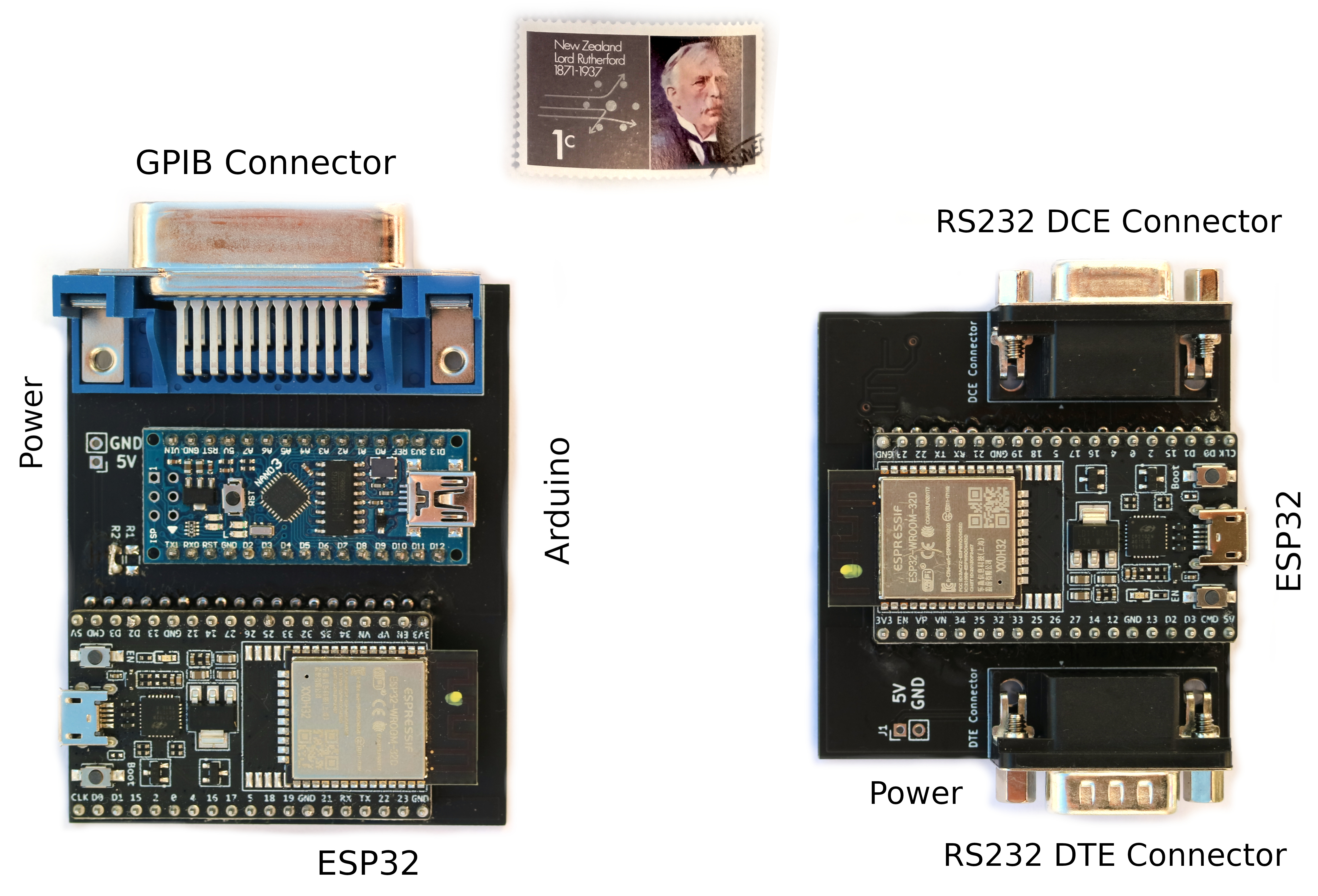
Fig. 4: Left: Our wireless GPIB interface which, for example, we use to monitor the power supplies of our electromagnets. The ESP32 uses an Arduino Nano to interface with GPIB. Right: Our wireless RS232 interface which, for example, we use to monitor a commercial laser controller. The module acts as Data Terminal Equipment (DTE), but many scientific instruments are wired as DTE, so it also features a Data Communications Equipment (DCE) wired connector to avoid the need for a null-modem cable. The MAX202 used to drive these serial interfaces is located on the reverse side of the board. A postage stamp is shown for size reference.

Commercial instruments are often outfitted with a digital serial interface for remote control and diagnostics. These interfaces, e.g. RS232, RS485 or GPIB, generally provide the ability to query the status of the device (e.g. via SCPI). Despite the obvious usefulness of wireless GPIB/serial interfaces [35, 36], curiously, commercial vendors do not provide solutions with integrated wireless capabilities, but invariably require a wireless router on top of an already costly GPIB-to-Ethernet interface [37, 38]. The cost of the latter can range from $200 to $1600 depending on supplier. As an attractive and more compact alternative, we provide a solution which integrates GPIB-to-WiFi on a single printed circuit board (PCB), with a total component cost that is less than $20.

To connect the ESP controller to the communication port of a commercial instrument, we need a protocol translator capable of handling and generating the voltage range of the interface bus. GPIB or IEEE-488 is a parallel bus interface, which only requires TTL signal levels. To manage this bus, we add an ATmega328P on an Arduino Nano 3 [34] board, following a design provided by Ref. [35]. This extra component acts as a level-shifter, and a serial-to-parallel converter, making the system GPIB compatible. We avoid using more powerful line drivers, which would be required for driving a GPIB bus with many instruments—our largest single bus has 3 instruments—and leave our setup “GPIB compatible”, rather than fully compliant with relevant GPIB specifications. The ESP controller and Arduino are assembled on a custom PCB with the appropriate connector to plug straight into an instrument (see Table 1). The board can be powered from a $5\text{\,}\mathrm{V}$ supply via the exposed header, or the USB ports on the Arduino or ESP development board.

For RS232, we use the MAX202 [39], which is a TTL-to-RS232 adapter. RS232 devices must be able to withstand a short-circuit to ground, and incoming voltages of up to $\pm$25\text{\,}\mathrm{V}$$, which are constraints the ESP controller cannot satisfy, but the MAX202 can. The MAX202 additionally contains a charge pump doubler and inverter to produce signals of $\pm$10\text{\,}\mathrm{V}$$ from the $5\text{\,}\mathrm{V}$ power supplied. We also use a custom PCB for this module. IEEE-488 and RS-232 are industry standards that have been used in test instrumentation since the 1960s for automation and control. Our system therefore opens up the very attractive possibility of retrofitting old high-end equipment with wireless monitoring and controlling capabilities.

3 Publishing Data to Server

The sensor modules connect to an MQTT service [40, 41] to which they transmit data (see Fig. 2). This service runs on a networked computer in the lab, which forms our data collection server. Data messages are sent as strings from each sensor module to the service with the value and units of each measurement. The messages are ‘published’ to different ‘topics’ on the server, which differentiates each signal being monitored. Other clients are then able to ‘subscribe’ to the ‘topics’, and receive the measurements.

When first deployed, a sensor module initially starts up its own WiFi network and awaits configuration from a web-browser (a mobile phone can be used for this purpose). This configuration specifies the SSID and password for the WiFi network to which the data collection server is connected, as well as the address of the server. Once configured, the device’s network disappears, and the module starts transmitting data.

In order for the data to be useful for analysis, we must have a way of storing it. We use the “agent” program Telegraf [42] to collect the data messages and store them in a time-series database, InfluxDB [43]. The data flow is shown in Fig. 2.

3.1 Other Data Sources

It is straightforward to send measurements to the message queuing service from sources other than our sensor modules, as the messages are transported in a simple string format, and the message queue interface is an open standard with many implementations available. Instruments that have USB, FireWire or network interfaces do not lend themselves easily to interfacing with the ESP controllers, but using suitable drivers for these instruments connected to a computer (e.g., a small Raspberry Pi single board computer), one can upload measurements to the message queue component of the monitoring system to take advantage of the analysis tools described in the following sections.

With an appropriate front-end, events can also be published to the server from direct user input via a web browser, e.g. from a cell phone. Examples of relevant events include periodic servicing maintenance tasks such as filter and lubricant replacement. Recently we have included the logging of shared equipment sterilization prompted by regulations put in place due to the COVID-19 pandemic. COVID-19 also introduced an acute requirement for contact tracing of laboratory personnel. We therefore currently log the user occupation of the laboratory, with a sign-in board built using NodeRED, a tool we also use for real-time analysis as discussed below.

4 Front End / Action Analysis

The setup we describe uses separate tools for real-time analysis, and for interacting with historical data (i.e., data stored in the InfluxDB database). Details on the services and their configuration can be found with our code [30].

Here we explain the user-facing tools that we use.

4.1 Visualisation

To visualise the data stored in the InfluxDB database we use Grafana [44] which offers “drag and drop” construction of monitoring dashboards and database queries. Grafana is accessed via a web-browser, allowing users to view the data remotely and from multiple computers simultaneously. It can also be made publicly and globally accessible via the internet, as we have done [45].

Grafana provides a number of ways of visualising data as ‘panels’ on a dashboard. Fig. 5 shows a simple example using graph and gauge panels. Grafana includes other panel types including bar gauges, tables, and heat maps. With these tools, one can create “control panel” type displays, or even “digital checklists”, where the operating state is indicated by colour, quickly highlighting anything that is not operating normally. Grafana supports multiple dashboards, and one can set the display to automatically change through them to get a live overview of the system. Grafana also offers a simple way for users to query and export data, avoiding having to interface with the database directly.

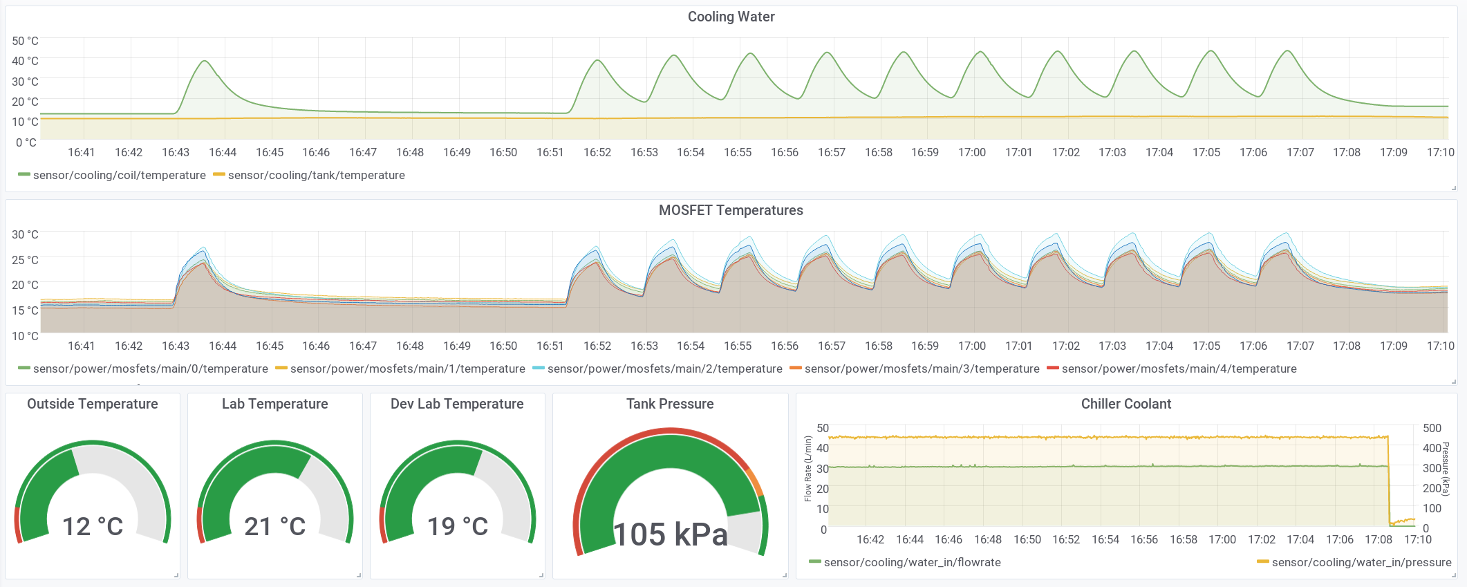
Fig. 5: Screenshot of a monitoring dashboard built using Grafana. The top graph shows the temperature of our cooling water in a storage tank, and coming out of a electromagnet coil. The middle plot shows the temperature of MOSFETs used for controlling current. The bottom row has several gauge panels, with the green colour indicating normal operating points. The lower plot is the cooling water supply flow-rate and pressure. Reference [45] provides a link to a live instance of our monitoring system.

4.2 Real-time Analysis

Our real-time analysis operates on data received from the message queue server directly, so detects if there is a fault with the experiment as soon as the data comes in. If a fault is detected, we may either wish to avoid wasting time collecting faulty experimental data, or we may try to act to correct the failure or minimise damage caused by the failure. The last point is the realm of safety devices (e.g. thermal fuses), and while it is not recommended to displace hardware interlocks and fail-safes, real-time analysis opens up interesting ways to augment these. An advantage of using the monitoring system to perform these tasks is the large amount of data available. For example, one may use data from multiple sensors simultaneously, e.g. differential flow rates between source and return lines can detect a leak.

For real-time analysis we use NodeRED [46] which runs on the data collection server and provides a web-based graphical and JavaScript programming environment for reacting to messages from the message queuing server. In NodeRED, messages are interpreted by a stream processing pipeline. In our setup, anomalies are primarily detected by determining when directly monitored quantities, or their combination, move outside set limits for normal operating values. For example, as the filter in our cooling water inlet gets dirty, the flow rate of water will slowly reduce over time and once it falls below a lower limit the monitoring system flags this. In addition, some parameters are compared against the average of recent values to detect sudden variations. An occurence of a leak or a blockage in a branch of our multi-stranded cooling water supply may not cause the oveall flow rate to move outside the set limits, but will give rise to an abrupt change. More complex sensor fusion and feature extraction are possible within the NodeRED framework, but we have found simple measures sufficient for detecting failures in our ultracold atom machine.

We use NodeRED to perform some preventative actions, such as shutting off our coolant pump if the system detects a leak or if the coolant tank is low. We can also disable the power supplies if the electromagnets being cooled get too warm or if the flow rate drops off. It is worth again noting that, especially the last two of these, should have dedicated hardware interlocks to act as a fail-safe. Real-time analysis is not meant as a replacement for proper safety design, but can take action to avoid the need to replace thermal fuses. Additionally, it can notify the user that there has been a fault, and where the fault occurred. In our setup, faults are displayed on Grafana, a custom LED character display at the experiment controls, and also sent out via Discord.

To take preventative actions we must have some devices capable of effecting control over parts of the experiment. While we have focused on the monitoring uses of our sensor modules, they are equally capable of producing a control signal. Typical examples include controlling relays, as shown in Fig. 2, or triggering interlock circuits. Hence the modules provide a way to react to changes in the experiment, such as turn off a pump if a leak is detected.

The above control examples produce digital signals using the GPIO pins. The ESP32 includes an on-chip digital-to-analog converter to produce analog signals. The ESP8266 does not have an on-chip converter, but one can be formed with pulse-width modulation and an output filter.

5 Demonstrations

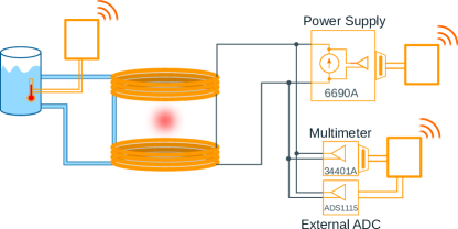
Fig. 6: A test configuration for our system. A power supply sources a current to our quadrupole electromagnets, trapping a cloud of cold atoms in the resulting magnetic field. The coil voltage is monitored by the power supply itself, a GPIB compatible multi-meter, and an ADS1115 ADC. The electromagnets are cooled by a recirculating water system (chiller and pumps not pictured), with the temperature of the coolant tank monitored.

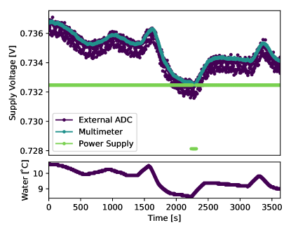
Fig. 7: Top panel: The voltage of the power supply for our the magnetic field coils of our quadrupole trap as measured in three different ways (see Fig. 6). The power supply readout is not sufficiently sensitive to detect the drifts which are recorded by the external ADC and the 6.5 digit multi-meter. Bottom panel: The temperature of recirculating cooling water flowing in the hollow copper tubing of the coils as measured in the storage tank by a wireless module (see Fig. 6).

5.1 Comparison of Data Sources

As a demonstration of our monitoring system, we use the setup in Fig. 6 to simultaneous log the voltage over a magnetic field coil pair and the temperature of cooling water flowing in the coils’ hollow copper windings. The coils are driven at a constant current by a commercial power supply (Keysight 6690A) and for demonstration purposes we monitor the voltage drop in three ways: using the module in Fig. 3(e) the supply voltage is monitored on one channel of an ADS1115 ADC , and using the wireless GPIB modules of Fig. 4(a), we poll the power supply itself as well as an external Keysight 34401A 6.5-digit multi-meter. The temperature of the cooling water supplied to the coils is monitored with the module in Fig. 3(a).

Figure 7 shows the data generated by the four detection modules of Fig. 6 and collected by our monitoring system over the course of an hour. Both the external ADC and the multi-meter are sufficiently sensitive to pick up the drift in the power supply voltage as it attempts to source a constant $35\text{\,}\mathrm{A}$ current. The voltage fluctuations measured using both these modules correlate highly with the temperature of the water cooling the coils, suggesting that we are observing the change of resistance due to temperature variation, with a coefficient of $51.2(1)\text{\,}\mathrm{\SIUnitSymbolMicro\SIUnitSymbolOhm}\text{\,}{\mathrm{K}}^{-1}$.

This example showcases the flexibility of our system. For simply detecting a fault in the coil, the coarse readings from directly polling the power supply itself via a wireless module would be sufficient to detect an open or short circuit. Using an ADC module, we can detect more subtle variations in process parameters that might correlate from one end of the ultracold atom machine to the other. Finally, using our wireless GPIB module we can achieve the accuracy provided by a 6.5 digit commercial state-of-the-art voltmeter (Agilent 34401A) with a traceble calibration.

5.2 Appending a spectrum analyzer

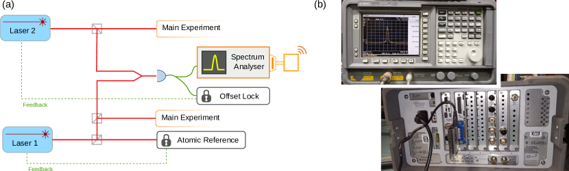
Fig. 8: (a) Light from two lasers is combined to produce a beat-note on a photodiode. As the frequency of Laser 1 is locked to an atomic reference, the beat-note is used to lock the frequency of Laser 2. Additionally, we monitor the beat-note with a spectrum analyser controlled via GPIB from our sensor module. (b) The front and rear view of the spectrum analyser, showing showing the the beat-note signal on the display, and the compact wireless sensor module connected to the GPIB interface.

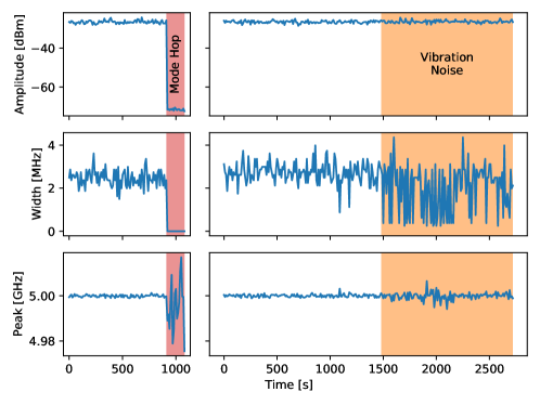
Fig. 9: The amplitude, linewidth, and centre frequency of the beat-note between two lasers, which are controlled such that the centre frequency is fixed at $5\text{\,}\mathrm{GHz}$. These observations show two areas of interest. In the red-shaded region, the laser has experienced a mode-hop, and the beat-note jumps out of range of the detector. In the orange-shaded region, an actively cooled RF source/amplifier is placed near the laser, coupling some vibration to the laser. The measured width becomes erratic as the beat-note moves around during a sweep of the spectrum analyser.

Ultra-cold atom machines make extensive use of narrow-linewidth, tunable light to cool and probe atomic samples. The lasers producing this light are typically frequency locked to atomic references using absorption spectroscopy. With one laser tied to an atomic spectroscopic line, other slave lasers may be locked to this master through a so-called beat-note or offset lock [47, 48]. Here, a phase detector compares the beat-note between the two lasers with a local oscillator. This offers an agile way of tuning the frequency of the slave laser, which can be offset by several GHz from the master. In our lab, we have found this particularly useful for dispersive optical probing of ultracold samples, where the probe light needs to be detuned far away from absorption resonances [49]. Prior to the implementation of our condition monitoring system, we would manually assess the quality of a beat-note lock using an Agilent E4405A Spectrum analyser. This is an example of a high-end legacy instrument with exceptional performance but with communication limited to GPIB. Using our wireless GPIB interface described in section 2.6, we poll the amplitude, width and peak frequency of the beat-note between a master and slave laser as shown in Fig. 8, and broadcast the values to the message queue of our monitoring system. Figure 9 shows two periods of traced data, highlighting two classes of events. In the red region, the slave laser experienced a mode-hop, resulting in the complete disappearance of the beat-note within the span monitored by the spectrum analyser. In contrast to such an obvious event which is fatal to an atomic experiment, we can also observe more subtle effects: the orange shaded region shows a decrease in laser stability that arose from the introduction of an RF source and amplifier near the laser, which we have attributed to vibrations introduced by a cooling fan.

6 Conclusion

We have reported on a condition monitoring system targeted at the research laboratory. Our platform operates with wireless sensor modules distributed around the lab and feeding into a message queuing service along with other data sources. The modules are all based on wireless ESP microcontrollers that interface both with home-built sensors and with commercial laboratory equipment which are annexed by the monitoring system. This latter, distinctive feature can lease a new life to legacy, high-end equipment. The present work provides a vehicle for detecting acute equipment failures and for providing information that quickly highlights the point of failure. It also provides a framework for logging process parameters and operating points of the day-to-day running of the experiments .

We have considered the specific example of an ultracold atom machine and used this as a test bed, but our monitoring system is suitable for a range of similarly complex experimental setups. The system is easily deployed and detailed instructions are provided to do this [30], making collecting information about an experiment’s condition a small investment. The code we developed for this project [30] is open-source, and uses third-party open-source libraries and tools. We hope that our work this will stimulate further development of this project.

Appendix A Supplementary material

A supplementary note discussing the voltage tolerance of the ESP System-on-Chips and documenting the ADC non-linearity of the ESP32 can be found online at (to be inserted by the editor). Code and detailed documentation for this project are available online [30]. This includes ready-to-use resources—sensor module firmware, service automation, and PCB designs for manufacture—and gives detailed documentation on how to replicate our monitoring system. .

References

- [1] L. Fallani, A. Kastberg, Cold atoms: A field enabled by light, EPL (Europhysics Letters) 110 (2015) 53001.
- [2] E. W. Streed, A. P. Chikkatur, T. L. Gustavson, M. Boyd, Y. Torii, D. Schneble, G. K. Campbell, D. E. Pritchard, W. Ketterle, Large atom number Bose-Einstein condensate machines, Rev. Sci. Instrum. 77 (2006) 023106.
- [3] H. J. Lewandowski, D. M. Harber, D. L. Whitaker, E. A. Cornell, Simplified system for creating a Bose-Einstein condensate, J. Low Temp. Phys. 132 (2003) 309–367.
- [4] O. Krarup, Imaging single atoms in an optical lattice, Master’s thesis, Aarhus University (2018).
- [5] G. Vachtsevanos, F. Lewis, M. Roemer, A. Hess, B. Wu, Intelligent Fault Diagnostrics and Prognosis for Engineering Systems, John Wiley and Sons, Inc, 2006.
- [6] J. Gubbi, R. Buyya, S. Marusic, M. Palaniswami, Internet of Things (IoT): A vision, architectural elements, and future directions, Future Generation Computer Systems 29 (2013) 1645–1660.
- [7] W.-T. Sung, S.-J. Hsiao, The application of thermal comfort control based on smart house system of IoT, Measurement 149 (2020) 106997.
- [8] L. Piwek, D. A. Ellis, S. Andrews, A. Joinson, The rise of consumer health wearables: Promises and barriers, PLOS Medicine 13 (2016) 1–9.
- [9] M. Akkaş, R. SOKULLU, H. E. Çetin, Healthcare and patient monitoring using IoT, Internet of Things 11 (2020) 100173.
- [10] R. Sokullu, M. A. Akkaş, E. Demir, IoT supported smart home for the elderly, Internet of Things 11 (2020) 100239.
- [11] F. Shrouf, J. Ordieres, G. Miragliotta, Smart factories in industry 4.0: A review of the concept and of energy management approached in production based on the internet of things paradigm, in: 2014 IEEE International Conference on Industrial Engineering and Engineering Management, 2014, pp. 697–701.
- [12] L. Hou, N. W. Bergmann, Novel industrial wireless sensor networks for machine condition monitoring and fault diagnosis, IEEE Trans. Instrum. Meas. 61 (2012) 2787–2798.
- [13] A. Bergeron, N. Baddour, Design and development of a low-cost multisensor inertial data acquisition system for sailing, IEEE Trans. Instrum. Meas. 63 (2014) 441–449.
- [14] M. Razfar, J. Castro, L. Labonte, R. Rezaei, F. Ghabrial, P. Shankar, E. Besnard, A. Abedi, Wireless network design and analysis for real time control of launch vehicles, in: IEEE International Conference on Wireless for Space and Extreme Environments, 2013, pp. 1–2.
- [15] L. Lombardo, S. Corbellini, M. Parvis, A. Elsayed, E. Angelini, S. Grassini, Wireless sensor network for distributed environmental monitoring, IEEE Trans. Instrum. Meas. 67 (2018) 1214–1222.
- [16] P. T. Lam, T. Q. Le, N. N. Le, S. D. Nguyen, Wireless sensing modules for rural monitoring and precision agriculture applications, Journal of Information and Telecommunication 2 (2018) 107–123.
- [17] B. T. W. Putra, New low-cost portable sensing system integrated with on-the-go fertilizer application system for plantation crops, Measurement 155 (2020) 107562.
- [18] O. Casas, M. López, M. Quílez, X. Martinez-Farre, G. Hornero, C. Rovira, M. R. Pinilla, P. M. Ramos, B. Borges, H. Marques, P. S. Girão, Wireless sensor network for smart composting monitoring and control, Measurement 47 (2014) 483–495.
- [19] N. Harris, A. Cranny, M. Rivers, K. Smettem, E. G. Barrett-Lennard, Application of distributed wireless chloride sensors to environmental monitoring: Initial results, IEEE Trans. Instrum. Meas. 65 (2016) 736–743.
- [20] A. G. Orozco-Lugo, D. C. McLernon, M. Lara, S. A. R. Zaidi, B. J. González, O. Illescas, C. I. Pérez-Macías, V. Nájera-Bello, J. A. Balderas, J. L. Pizano-Escalante, C. M. Perera, R. Rodríguez-Vázquez, Monitoring of water quality in a shrimp farm using a FANET, Internet of Things (2020) 100170.
- [21] V. V. Khoa, S. Takayama, Wireless sensor network in landslide monitoring system with remote data management, Measurement 118 (2018) 214–229.
- [22] P. Giri, K. Ng, W. Phillips, Wireless sensor network system for landslide monitoring and warning, IEEE Trans. Instrum. Meas. 68 (2019) 1210–1220.
- [23] A. Rakonjac, A. B. Deb, S. Hoinka, D. Hudson, B. J. Sawyer, N. Kjærgaard, Laser based accelerator for ultracold atoms, Opt. Lett. 37 (2012) 1085.
- [24] A. B. Deb, B. J. Sawyer, N. Kjærgaard, Dispersive probing of driven pseudospin dynamics in a gradient field, Phys. Rev. A 88 (2013) 063607.
- [25] A. B. Deb, T. McKellar, N. Kjærgaard, Optical runaway evaporation for the parallel production of multiple bose-einstein condensates, Phys. Rev. A 90 (2014) 051401.
- [26] C. S. Chisholm, R. Thomas, A. B. Deb, N. Kjærgaard, A three-dimensional steerable optical tweezer system for ultracold atoms, Rev. Sci. Instrum. 89 (2018) 103105.
- [27] R. Thomas, M. Chilcott, E. Tiesinga, A. B. Deb, N. Kjærgaard, Observation of bound state self-interaction in a nano-eV atom collider, Nat. Commun. 9 (2018) 4895.
- [28] B. J. Sawyer, M. Chilcott, R. Thomas, A. B. Deb, N. Kjærgaard, Deterministic quantum state transfer of atoms in a random magnetic field, Eur. Phys. J. D 73 (2019) 160.
- [29] S. J. Moore, C. D. Nugent, S. Zhang, I. Cleland, IoT reliability: a review leading to 5 key research directions, CCF Transactions on Pervasive Computing and Interaction 2 (2020) 147–163.
-
[30]
M. Chilcott, Monitoring
system source code, and internal documentation (2019).
URL https://github.com/kjaergaard-lab/lab-monitor -
[31]
NodeMcu Team, NodeMCU
devkit v1.0 (2019).
URL https://github.com/nodemcu/nodemcu-devkit-v1.0 -
[32]
PlatformIO, An open source ecosystem for IoT
development (2019).
URL https://platformio.org/ - [33] Maxim Integrated, DS18B20 datasheet (2018).
-
[34]
Arduino, Arduino (2019).
URL https://www.arduino.cc/ -
[35]
AR488 Arduino GPIB Interface,
2019.
URL https://github.com/Twilight-Logic/AR488 - [36] N. Quinteiro, Wirelessly accessing instruments with standard GPIB/WLAN interfaces, Bachelor’s thesis, HES-SO Valais-Wallis (2014).
-
[37]
National Instruments, Developing
wireless gpib test systems using ni ethernet-to-gpib controllers (2017).
URL http://www.ni.com/tutorial/3279/en/ -
[38]
Agilent Technologies,
Setting
up a wireless connection for the Agilent 34450a 5 digit
multimeter (2013).
URL https://literature.cdn.keysight.com/litweb/pdf/34450-90032.pdf - [39] Texas Instruments, MAX202 5-V dual RS-232 line driverand receiver with 15-kV ESD protection (2020).
-
[40]
Eclipse Foundation, Eclipse mosquitto (2019).
URL https://mosquitto.org/ -
[41]
Organization for the Advancement of Structured Information Standards,
Mqtt
specification (v5.0) (2019).
URL https://docs.oasis-open.org/mqtt/mqtt/v5.0/mqtt-v5.0.html -
[42]
InfluxData Inc., Influxdata
products (2019).
URL https://www.influxdata.com/products/ -
[43]
InfluxData Inc.,
Influxdb
(2019).
URL https://www.influxdata.com/products/influxdb-overview/ -
[44]
Grafana Labs, Grafana (2019).
URL https://grafana.com/ - [45] Our Grafana instance is visible at http://hoodoo.otago.ac.nz/mattlab/ at the time of print. (2019).
-
[46]
NodeRED Project, Nodered (2019).
URL https://nodered.org/ - [47] Y. Seishu, T. Hasegawa, Robust offset locking of laser frequency with electronically tunable LC circuits for sub-millihertz uncertainty, Applied Physics B 125 (2019) 142.
- [48] J. Appel, A. MacRae, A. I. Lvovsky, A versatile digital GHz phase lock for external cavity diode lasers, Measurement Science and Technology 20 (2009) 055302.
- [49] B. J. Sawyer, M. S. J. Horvath, E. Tiesinga, A. B. Deb, N. Kjærgaard, Dispersive optical detection of magnetic feshbach resonances in ultracold gases, Physical Review A 96 (2017) 022705.