Cell-Free Massive MIMO
for Wireless Federated Learning

Tung T. Vu, Duy T. Ngo, Nguyen H. Tran, Hien Quoc Ngo, Minh N. Dao, and Richard H. Middleton Manuscript received December 18, 2019; revised April 21, 2020; accepted June 10, 2020. The editor coordinating the review of this paper and approving it for publication was Ming Xiao.Tung T. Vu was supported by an ECR-HDR scholarship from The University of Newcastle. Duy T. Ngo was supported in part by the Australian Research Council Discovery Project (ARCDP) grant DP170100939, and in part by the Vietnam National Foundation for Science and Technology Development (NAFOSTED) under grant number 102.02-2018.320. Nguyen H. Tran was supported in part by the ARCDP grant DP200103718, and in part by NAFOSTED under grant number 102.02-2019.321. H. Q. Ngo was supported by the UK Research and Innovation Future Leaders Fellowships under Grant MR/S017666/1. Minh N. Dao was partially supported by ARCDP grants DP160101537 and DP190100555.T. T. Vu, D. T. Ngo and R. H. Middleton are with the School of Electrical Engineering and Computing, The University of Newcastle, Callaghan, NSW 2308, Australia (e-mail: thanhtung.vu@uon.edu.au; {duy.ngo, richard.middleton}@newcastle.edu.au).N. H. Tran is with the School of Computer Science, The University of Sydney, Sydney, NSW 2006, Australia (e-mail: nguyen.tran@sydney.edu.au).H. Q. Ngo is with the School of Electronics, Electrical Engineering and Computer Science, Queen’s University Belfast, Belfast BT7 1NN, United Kingdom (e-mail: hien.ngo@qub.ac.uk).M. N. Dao is with the Department of Applied Mathematics, The University of New South Wales, Sydney, NSW 2052, Australia (e-mail: daonminh@gmail.com).
Abstract

This paper proposes a novel scheme for cell-free massive multiple-input multiple-output (CFmMIMO) networks to support any federated learning (FL) framework. This scheme allows each instead of all the iterations of the FL framework to happen in a large-scale coherence time to guarantee a stable operation of an FL process. To show how to optimize the FL performance using this proposed scheme, we consider an existing FL framework as an example and target FL training time minimization for this framework. An optimization problem is then formulated to jointly optimize the local accuracy, transmit power, data rate, and users’ processing frequency. This mixed-timescale stochastic nonconvex problem captures the complex interactions among the training time, and transmission and computation of training updates of one FL process. By employing the online successive convex approximation approach, we develop a new algorithm to solve the formulated problem with proven convergence to the neighbourhood of its stationary points. Our numerical results confirm that the presented joint design reduces the training time by up to 55%percent5555\% over baseline approaches. They also show that CFmMIMO here requires the lowest training time for FL processes compared with cell-free time-division multiple access massive MIMO and collocated massive MIMO.

Index Terms:
Cell-free massive MIMO, federated learning.

I Introduction

The use of machine learning (ML) techniques in telecommunications industry has been growing dramatically in recent years [1, 2]. One reason for this trend is the fast growing number of mobile devices, wearable devices and autonomous vehicles. They are generating a vast amount of data by using in-built sensors, e.g., microphones, GPS and camera, for critical applications such as traffic navigation, indoor localization, image recognition, natural language processing, and augmented reality [3]. In addition, the computational capabilities of these devices also grow significantly with dedicated hardware architecture and computing engines, e.g., the energy-efficient Qualcomm Hexagon Vector eXtensions on Snapdragon 835835835 [4]. On-device artificial intelligence (AI) capabilities are predicted to be available on 80%percent8080\% of all smartphones by 202220222022 [5]. It is therefore critical for telecommunications operators to start investigating into a future communications system that efficiently utilizes the empowered computation resources from mobile devices to solve ML problems.

The typical ML framework used in the current telecommunications systems requires a cloud center to store and process raw data collected by the user equipment (UEs). However, such a centralized structure fails to support real-time applications because of its high latency [6]. The concept of mobile edge computing is introduced to process data at the edge nodes instead of the cloud center [7, 8]. Since the computational capability of mobile devices is growing noticeably, it is possible to even push the network computation further to the mobile device level [9, 10]. On the other hand, serious concerns about data privacy have recently been raised due to data being processed by third-party companies, e.g., Facebook, Apple. This urgently calls for a new class of ML frameworks that not only exploit the computational resources of the UEs for ML applications but also ensure data privacy.

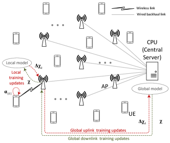
A promising candidate for such ML frameworks is the recently developed Federated Learning (FL) [9, 11]. As shown in Fig. 1, an FL process is an iterative process in which the UEs use their local training data to compute local model training updates, followed by sending the updates to a central server. The central server then aggregates these updates to compute the global training update, which is then sent back to the UEs to further assist their local update computation. This iterative process terminates when a certain learning accuracy level is attained. Data privacy is protected by not sharing the local training data, but only the local training updates computed at the UEs using local computational resources. Uploading only the local training updates to the central server incurs a significantly lower delay, compared to uploading a large amount of raw data. This distributed approach facilitates a large-scale model training and more flexible data collection, albeit at the expense of UEs’ computational resources [10].
Refer to caption
Figure 1: Illustration of an FL process over communication networks and CFmMIMO network model used to support FL.

With all the promising advantages listed above, FL has attracted much attention from both developer and researcher communities [12, 13, 14, 15, 10, 16, 17]. In [12], an FL algorithm for keyboard prediction on smartphones is developed by Google. [13] target improving the performance of the general FL algorithms, while [14, 15, 16, 10, 17] concentrate on optimizing the performance of FL algorithms used in wireless networks. In particular, [13] proposes a new compression framework for a communication-efficient FL system. [10] aims to obtain the best trade-off between FL training time and UE energy consumption. [14] proposes an incentive mechanism that encourages the UEs with high-quality data to participate in FL systems. [15] introduces a control algorithm to achieve the best trade-off between the number of local updates and that of global updates for a given resource budget. A joint device selection and beamforming design is proposed in [16] to enhance the performance of FL. [17] proposes a joint design of user selection, power control and subchannel allocation for minimizing the loss function of FL.

This paper investigates how to implement FL in a wireless network. It is worth noting that the existing works [10, 16] rely on an impractical assumption that the channel state information (CSI) remains unchanged during the whole FL process. In practice however, the channel changes in the order of milliseconds; and as such, certain system parameters for FL performance optimization, e.g., data rates and power control, would have become obsolete even before the FL process terminates. In addition, it might not be most efficient to use orthogonal multiplexing approaches, e.g., orthogonal frequency-division multiple access (OFDMA) [17] and time-division multiple access (TDMA) [10], for UEs to transmit their local updates. With a large number of UEs, the total training time could be significantly prolonged. To both deal with the wireless channel dynamics and to serve UEs at the same time and in the same frequency bands, a new wireless network structure that supports FL is called for.

In this work, we propose using cell-free massive multiple-input multiple-output (CFmMIMO) [18, 19] for FL in a wireless environment. Here, a central processing unit (CPU) (i.e., the central server) is connected to a large number of access point (APs) via backhaul links. These APs then simultaneously serve UEs via wireless links using the same frequency bands with the CSI acquired via uplink (UL) training pilots. An important characteristic of massive MIMO is channel hardening [20], i.e., the effective channel gain at the UEs is close to its expected value—a known deterministic constant [19]. As such, the channels are reasonably stable during one large-scale coherence time T~csubscript~𝑇𝑐\widetilde{T}_{c}111During one large-scale coherence time T~csubscript~𝑇𝑐\widetilde{T}_{c}, the large-scale fading coefficients are reasonably invariant. The value of T~csubscript~𝑇𝑐\widetilde{T}_{c} can be empirically measured, in the same way for small-scale fading measurement. For indoor communications, the large-scale coherence time can be at least 404040 small-scale fading coherence time [19], and it has a time order of seconds.. The channel dynamics due to small-scale fading thus have negligible effects on the FL processes. In addition, a CFmMIMO network also provides a high probability of coverage, making the FL processes less prone to the unfavorable UE links.

Our research contributions are summarized as follows.

  • We propose, for the first time, a scheme for CFmMIMO networks to support any FL framework. In this scheme, any iterative algorithm can be developed to optimize the FL performance before the FL process is executed. Each instead of all iterations of this FL optimization algorithm or the FL process happens within one T~csubscript~𝑇𝑐\widetilde{T}_{c} in order to guarantee channel stability during its operation. In each iteration of the FL process, we propose using the APs as relays to transmit the training updates between the CPU and UEs. Doing so allows any beamforming/filtering design to be applied to the APs in order to enhance the performance of training update transmission.

  • To show how to optimize the FL performance using the proposed scheme, we consider an existing FL framework [21] as an example and target the key performance metric of “training time minimization”. We formulate a mixed-timescale stochastic nonconvex optimization problem that minimizes the time of one FL process. The formulated problem captures the complex interactions among the FL training time, and transmission and computation of FL training updates in a CFmMIMO network. Here, a conjugate beamforming/matched filtering scheme is applied to the APs for ease of implementation. The local accuracy, power control, data rate and UE’s processing frequency are jointly designed, subject to the practical constraints on UEs’ energy consumption and imperfect channel estimation.

  • Utilizing the general framework in [22], we propose a new algorithm that is proven to converge to at least the neighborhood of the stationary points of the formulated problem. Here, the coupling among the variables makes it challenging to develop a specific algorithm that satisfies all the strict conditions stated in the general framework of [22]. It is also noted that our algorithm only requires channel stability in each but not all iterations. This important feature ensures the problem and its solution remain up-to-date and valid during the running time of the algorithm, despite the channel variations.

  • Simulation results verify the convergence of the proposed algorithm, and show that our solution reduces the training time by up to 55%percent5555\% compared with the baseline schemes. They further confirm that CFmMIMO offers the lowest training time compared to cell-free TDMA massive MIMO and collocated massive MIMO.

Paper Organization and Notation: The rest of this paper is organized as follows. Section II proposes a novel scheme for a CFmMIMO network to support a general FL framework. Section III introduces a specific example of the general FL framework considered in this paper. Section IV presents the system model and assumptions. Section V formulates the FL training time minimization problem, whereas Section VI proposes a new algorithm to solve the formulated problem. For comparison, Section VII introduces cell-free TDMA and collocated massive MIMO systems to also support the considered FL framework. Section VIII verifies the performance of the developed algorithm through comprehensive numerical examples. Finally, Section IX concludes the paper.

In this paper, boldfaced symbols are used for vectors and capitalized boldfaced symbols for matrices. 𝑿superscript𝑿\boldsymbol{X}^{*} and 𝑿Hsuperscript𝑿𝐻\boldsymbol{X}^{H} are the conjugate and conjugate transposition of a matrix 𝑿𝑿\boldsymbol{X}, respectively. dsuperscript𝑑\operatorname{\mathbb{R}}^{d} is a space where its elements are real vectors with length d𝑑d. 𝐱,𝐲𝐱𝐲\langle\operatorname{\boldsymbol{x}},\operatorname{\boldsymbol{y}}\rangle means the inner product of vectors 𝐱𝐱\operatorname{\boldsymbol{x}} and 𝐲𝐲\operatorname{\boldsymbol{y}}. ||.||||.|| denotes the 2subscript2\ell_{2}-norm function. 𝒞𝒩(𝝁,𝑸)𝒞𝒩𝝁𝑸\operatorname{\mathcal{CN}}(\boldsymbol{\mu},\boldsymbol{Q}) denotes the circularly symmetric complex Gaussian distribution with mean 𝝁𝝁\boldsymbol{\mu} and covariance 𝑸𝑸\boldsymbol{Q}. g𝑔\nabla g is the gradient of a function g𝑔g. 𝔼{x}𝔼𝑥\operatorname{\mathbb{E}}\{x\} denotes the expected value of a random variable x𝑥x.

II Proposed Scheme for CFmMIMO Networks to Support FL

II-A The General FL Framework

A global ML problem is solved at a central server with a global training data set partitioned over a number of participating clients. Each client trains their local model by an arbitrary learning algorithm. Let 𝒦={1,,K}𝒦1𝐾\operatorname{\mathcal{K}}=\{1,...,K\} be the set of clients and Dksubscript𝐷𝑘D_{k} the size of the local data stored at client k𝑘k. Then D~=k𝒦Dk~𝐷subscript𝑘𝒦subscript𝐷𝑘\widetilde{D}=\sum_{k\in\operatorname{\mathcal{K}}}D_{k} is the size of the global training data. Denote by 𝒟={1,,D~}𝒟1~𝐷\operatorname{\mathcal{D}}=\{1,...,\widetilde{D}\} and 𝒟k={1,,Dk}subscript𝒟𝑘1subscript𝐷𝑘\operatorname{\mathcal{D}}_{k}=\{1,...,D_{k}\} the index sets of the global data samples and the local data samples at a client k𝑘k, respectively. In a typical supervised learning, a data sample i𝒟𝑖𝒟i\in\operatorname{\mathcal{D}} is defined as an input-output pair {𝐱id,yi}subscript𝐱𝑖superscript𝑑subscript𝑦𝑖\{\operatorname{\boldsymbol{x}}_{i}\in\mathbb{R}^{d},y_{i}\}.

For λ>0𝜆0\lambda>0, the general global ML problem can be posed as the following minimization [11, 21]

min𝐰dJ(𝐰)1D~i𝒟fi(𝐰)+λg(𝐰),𝐰superscript𝑑𝐽𝐰1~𝐷subscript𝑖𝒟subscript𝑓𝑖𝐰𝜆𝑔𝐰\displaystyle\underset{\operatorname{\boldsymbol{w}}\in\mathbb{R}^{d}}{\min}\,\,J(\operatorname{\boldsymbol{w}})\triangleq\frac{1}{\widetilde{D}}\sum_{i\in\operatorname{\mathcal{D}}}f_{i}(\operatorname{\boldsymbol{w}})+\lambda g(\operatorname{\boldsymbol{w}}), (1)

where fi(𝐰)subscript𝑓𝑖𝐰f_{i}(\operatorname{\boldsymbol{w}}) is the loss function at data sample i𝑖i and g(𝐰)𝑔𝐰g(\operatorname{\boldsymbol{w}}) is a regularization term with a model parameter 𝐰𝐰\operatorname{\boldsymbol{w}}. Some popular examples are fi(𝐰)=12(𝐱iT𝐰yi)2subscript𝑓𝑖𝐰12superscriptsuperscriptsubscript𝐱𝑖𝑇𝐰subscript𝑦𝑖2f_{i}(\operatorname{\boldsymbol{w}})=\frac{1}{2}(\operatorname{\boldsymbol{x}}_{i}^{T}\operatorname{\boldsymbol{w}}-y_{i})^{2} for a linear regression problem and fi(𝐰)={0,1yi𝐱iT𝐰},yi{1,1}formulae-sequencesubscript𝑓𝑖𝐰01subscript𝑦𝑖superscriptsubscript𝐱𝑖𝑇𝐰subscript𝑦𝑖11f_{i}(\operatorname{\boldsymbol{w}})=\{0,1-y_{i}\operatorname{\boldsymbol{x}}_{i}^{T}\operatorname{\boldsymbol{w}}\},y_{i}\in\{-1,1\} for a support vector machine. Here, the learning problem is to find 𝐰𝐰\operatorname{\boldsymbol{w}} that characterizes the output yisubscript𝑦𝑖y_{i} with the loss function fi(𝐰)subscript𝑓𝑖𝐰f_{i}(\operatorname{\boldsymbol{w}}) for a given input 𝐱isubscript𝐱𝑖\operatorname{\boldsymbol{x}}_{i}. Note that fi(𝐰)subscript𝑓𝑖𝐰f_{i}(\operatorname{\boldsymbol{w}}) is not necessarily convex.

In a general FL framework to solve the general ML problem (1), this problem is decomposed into K𝐾K separate local ML problems that are solved at K𝐾K clients in parallel. For ease of presentation, we make the following definitions.

Definition 1.

“Global DL training update” is the information sent from the central server to the clients. Similarly, “global UL training updates” are those from the clients to the central server.

The general FL framework is described in Algorithm 1. Each iteration of Algorithm 1 consists the four key steps (S1)-(S4).

Definition 2.

“An FL process” is defined as a full execution of Algorithm 1.

Algorithm 1 A general FL framework
1:  Input: n=1𝑛1n=1, an initial global DL training update
2:  repeat
3:     (S1) The central server sends the global DL training update to the UEs.
4:     for k𝒦𝑘𝒦k\in\operatorname{\mathcal{K}} in parallel do
5:        (S2) Client k𝑘k updates and solves its local ML problem on its local data set and then computes the global UL training update
6:        (S3) Client k𝑘k sends its computed global UL training update to the central server
7:     end for
8:     (S4) The central server computes the global DL training update by aggregating the received UL training updates.
9:     Update n=n+1𝑛𝑛1n=n+1
10:  until convergence with the global accuracy ϵitalic-ϵ\epsilon

Remark 1.

The designs of local ML problems at the clients, the global DL/UL training updates, and the types of aggregation of training updates at the central server are different according to the different designs of FL frameworks for different types of objective functions due to different ML applications [23, 24, 25, 26, 21, 27].

II-B Proposed Cell-Free Massive MIMO Network Structure to Support the General FL Framework

Here, we propose using the CFmMIMO network structure [19] illustrated in Fig. 1 to support the general FL framework discussed above. In this structure, a central processing unit (CPU) is connected to a set of access points (APs) ={1,,M}1𝑀\operatorname{\mathcal{M}}=\{1,...,M\} via backhaul links with sufficient capacities. These APs serve a given set 𝒦𝒦\operatorname{\mathcal{K}} of participating UEs via wireless access links at the same time and in the same frequency bands222In general, since the UEs are geographically distributed, some user may loss the connectivity, and hence, cannot participate in the FL process. However, one of the main strong property of CFmMIMO is that, with very high probability, it can provide uniformly good service for all users in the networks [19]. In the other words, in CFmMIMO, the connectivity probability of each user is very high. Therefore, in the paper, for simplicity, we assume that all UEs participate in the FL process.. The APs and UEs are each equipped with a single antenna. The CPU and UEs act as the central server and the clients in the general FL framework, respectively. The APs are used to relay the training updates between the CPU and the UEs

Remark 2.

Both the AP and UEs can be considered as the clients in the general FL framework. In this paper, we choose the UEs to be the clients instead of the APs [10]. By doing so, data privacy is more protected since raw data does not have to be shared over wireless networks. Moreover, the computational resource of the UEs can be empowered with new computing engines such as Snapdragon 835835835 [4]. It is possible to push the ML tasks further to the UEs [9, 10].

II-C Proposed Scheme for a CFmMIMO to Support the General FL framework

Now, to realize an FL process in the considered CFmMIMO network structure, we propose a general scheme shown in Fig. 3. As seen from the figure, we divide the time period during which the statistics of large-scale fading is stable into multiple time intervals. The first interval of “FL performance optimization” is used for optimizing the performance of FL. The remaining intervals are reserved for the FL process; hence, termed as “FL process” intervals.

Refer to caption
Figure 2: Proposed scheme of a CFmMIMO system to support FL
Refer to caption
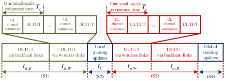
Figure 3: One iteration of the FL process

II-C1 Optimizing the performance of FL

In the “FL performance optimization” interval, any algorithms can be developed to optimize the performance of FL before the FL processes are executed. Here, we denote by “system parameters” the parameters that are designed by the FL optimization algorithm. These parameters are grouped into short-term and long-term parameters. The short-term parameters change in the timescale of large-scale coherence times, whereas the long-term parameters the statistics of large-scale fading. In each iteration of the optimization algorithm, the short-term parameters are designed in the short-term optimization (STO) time blocks, whereas the long-term parameters in the long-term optimization (LTO) time blocks. As a result of the channel hardening effect in massive MIMO, the wireless channel remains unchanged during one large-scale coherence time T~csubscript~𝑇𝑐\widetilde{T}_{c}. In practice, the completion time of the optimization algorithm can be larger than T~csubscript~𝑇𝑐\widetilde{T}_{c}. Therefore, we insist that only one iteration of the algorithm is to happen within T~csubscript~𝑇𝑐\widetilde{T}_{c}.

II-C2 Implementing the FL process

In the “FL process” intervals, the FL process is executed with the long-term parameters obtained from the “FL performance optimization” interval. The short-term parameters are optimized in the STO time block to enhance the performance of training update transmission before each iteration of the FL process. Since the completion time of the FL process can be larger than T~csubscript~𝑇𝑐\widetilde{T}_{c}, we insist that both STO and “one iteration of the FL process” time blocks are to happen in one T~csubscript~𝑇𝑐\widetilde{T}_{c}. Here, we note that the results of the LTO time blocks remain unchanged for several FL process, while the results of the STO time blocks are invariant only in one iteration of an FL process. Therefore, after the “FL performance optimization” step is executed, only the results of the LTO time block are used in FL processes. In each iteration of an FL process, the results of the STO time block are not the results of the STO time block in the “FL performance optimization” step, but rather are computed by the same method used for the STO time block in the “FL performance optimization” step.

II-C3 Implementing each iteration of the FL process

Fig. 3 shows the time block of “one iteration of the FL process”, in which the intervals of the four key steps (S1)-(S4) to implement each iteration of the FL process by the CFmMIMO network model are illustrated. Here, the interval of Step (S1) in Algorithm 1 consists one interval of “DL training update transmission (DLTUT) via backhaul links” from the CPU to the APs, and one interval of “DLTUT via wireless links” from the APs to the UEs. The interval of Step (S3) includes one interval of “UL training udpate transmission (ULTUT) via wireless links” from the UEs to the APs, and one interval of “ULTUT via backhaul links” from the APs to the CPU.

As also seen from Fig. 3, we split each time block of “DLTUT via wireless links” or “ULTUT via wireless links” into multiple intervals. The intervals of “UL training” is used for channel estimation. The remaining intervals are used for DL/UL training update transmission333The proposed scheme above focuses only on support FL. Therefore, in each small-scale coherence time, all the times not used to estimate the channel are used for transmitting training updates. The scheme that supports FL and data transmission at the same time is left for future works.. In these “DLTUT” or “ULTUT” intervals, any beamforming/filtering design can be applied to optimize the performance of training update transmission. Here, we insist that the pair of “UL training” and “DLTUT”/“ULTUT” intervals happen in one small-scale coherence time Tcsubscript𝑇𝑐T_{c} in order to adapt to the variation of small-scale fading444In this work, we consider time-division duplexing (TDD) where channels are first estimated at the APs via uplink channel estimation. Owing to the channel reciprocity property in massive MIMO, these channel estimates will then be used for: (i) precoding the data symbols in the downlink data transmission, and (ii) used for combining the received signals in the uplink data transmission. Moreover, there is no need for downlink channel estimation because of the channel hardening property in massive MIMO systems. This transmission protocol is widely used in the massive MIMO literature (see, e.g., [28]).. In addition, the data size of training updates may be larger than the amount of data that can be transmitted in Tcsubscript𝑇𝑐T_{c}. As such, there may be one or several “DLTUT” or “ULTUT” intervals in each “DLTUT via wireless links” or “ULTUT via wireless links” time block in order to complete the transmission of one global DL/UL training update.

Remark 3.

The proposed CFmMIMO network model in Section II-B and the proposed scheme in Section II-C can be used to support any version of the general FL framework to solve any global ML problem. This scheme only requires developing specific algorithms to optimize the performance of specific FL frameworks. In the following, we consider a specific example of the general FL framework and investigate an algorithm to optimize the FL performance of this framework.

III A Specific Example of the General FL Framework

Given the proposed framework in Section II, this section considers a specific example of the general FL framework to show how the performance of an FL process can be optimized in the latter sections. In particular, the FL optimization problem for this example is introduced in Section V, and the algorithms to solve this problem are proposed in Section VI.

Because of all the potential advantages offered by FL, many versions [23, 24, 25, 26, 21, 27] of the general FL framework have so far been studied despite research on FL is still in its infancy. Here, we consider an existing FL framework of [21] which is briefly introduced as follows. In this FL framework, the considered loss function fisubscript𝑓𝑖f_{i} is convex and the dual problem of (1) is written as

max𝜶D~JD~(𝜶)1D~i𝒟fi(𝜶)λg(𝝌(𝜶)),𝜶superscript~𝐷subscript𝐽~𝐷𝜶1~𝐷subscript𝑖𝒟superscriptsubscript𝑓𝑖𝜶𝜆superscript𝑔𝝌𝜶\displaystyle\underset{\operatorname{\boldsymbol{\alpha}}\in\mathbb{R}^{\widetilde{D}}}{\max}\,\,J_{\widetilde{D}}(\operatorname{\boldsymbol{\alpha}})\triangleq\tfrac{1}{\widetilde{D}}\sum_{i\in\operatorname{\mathcal{D}}}-f_{i}^{*}(-\operatorname{\boldsymbol{\alpha}})-\lambda g^{*}(\operatorname{\boldsymbol{\chi}}(\operatorname{\boldsymbol{\alpha}})), (2)

which is a special case of the Fenchel duality [21], where fisubscriptsuperscript𝑓𝑖f^{*}_{i} and gsuperscript𝑔g^{*} are the convex conjugate functions of fisubscript𝑓𝑖f_{i} and g𝑔g, respectively; 𝜶𝜶\operatorname{\boldsymbol{\alpha}} is a dual variable; 𝝌(𝜶)=1λD~𝐗𝜶𝝌𝜶1𝜆~𝐷𝐗𝜶\operatorname{\boldsymbol{\chi}}(\operatorname{\boldsymbol{\alpha}})=\tfrac{1}{\lambda\widetilde{D}}\operatorname{\boldsymbol{X}}\operatorname{\boldsymbol{\alpha}}; 𝐗=[𝐱1,,𝐱D~]d×D~𝐗subscript𝐱1subscript𝐱~𝐷superscript𝑑~𝐷\operatorname{\boldsymbol{X}}=[\operatorname{\boldsymbol{x}}_{1},...,\operatorname{\boldsymbol{x}}_{\widetilde{D}}]\in\mathbb{R}^{d\times\widetilde{D}}. It can be shown that if 𝜶superscript𝜶\operatorname{\boldsymbol{\alpha}}^{*} is an optimal solution of (2), then 𝐰(𝜶)=g(1λD~𝐗𝜶)𝐰superscript𝜶superscript𝑔1𝜆~𝐷𝐗superscript𝜶\operatorname{\boldsymbol{w}}(\operatorname{\boldsymbol{\alpha}}^{*})=\nabla g^{*}\big{(}\tfrac{1}{\lambda\widetilde{D}}\operatorname{\boldsymbol{X}}\operatorname{\boldsymbol{\alpha}}^{*}\big{)} is the optimal solution of (1). This property allows handling the dual variable 𝜶D~𝜶superscript~𝐷\operatorname{\boldsymbol{\alpha}}\in\mathbb{R}^{\widetilde{D}} instead of 𝐰d𝐰superscript𝑑\operatorname{\boldsymbol{w}}\in\mathbb{R}^{d}. Since each αisubscript𝛼𝑖\alpha_{i} corresponds to each data sample i𝑖i, 𝜶𝜶\operatorname{\boldsymbol{\alpha}} can be distributed in the same way that data are partitioned for the K𝐾K clients.

Let (ϕ)isubscriptbold-italic-ϕ𝑖(\operatorname{\boldsymbol{\phi}})_{i} be the i𝑖i-th element of vector ϕbold-italic-ϕ\operatorname{\boldsymbol{\phi}} and (𝐗)isubscript𝐗𝑖(\operatorname{\boldsymbol{X}})_{i} be the i𝑖i-th column vector of matrix 𝐗𝐗\operatorname{\boldsymbol{X}}. For any ϕD~bold-italic-ϕsuperscript~𝐷\operatorname{\boldsymbol{\phi}}\in\mathbb{R}^{\widetilde{D}}, denote by ϕ[k]D~subscriptbold-italic-ϕdelimited-[]𝑘superscript~𝐷\operatorname{\boldsymbol{\phi}}_{[k]}\in\mathbb{R}^{\widetilde{D}} the vector for device k𝑘k, i.e., (ϕ[k])i=(ϕ)isubscriptsubscriptbold-italic-ϕdelimited-[]𝑘𝑖subscriptbold-italic-ϕ𝑖(\operatorname{\boldsymbol{\phi}}_{[k]})_{i}=(\operatorname{\boldsymbol{\phi}})_{i} if i𝒟k𝑖subscript𝒟𝑘i\in\mathcal{D}_{k} and 00 otherwise. Similarly, for any 𝐗d×D~𝐗superscript𝑑~𝐷\operatorname{\boldsymbol{X}}\in\mathbb{R}^{d\times\widetilde{D}}, denote by 𝐗[k]d×D~subscript𝐗delimited-[]𝑘superscript𝑑~𝐷\operatorname{\boldsymbol{X}}_{[k]}\in\mathbb{R}^{d\times\widetilde{D}} the matrix for device k𝑘k, i.e., (𝐗[k])i=(𝐗)isubscriptsubscript𝐗delimited-[]𝑘𝑖subscript𝐗𝑖(\operatorname{\boldsymbol{X}}_{[k]})_{i}=(\operatorname{\boldsymbol{X}})_{i} if i𝒟k𝑖subscript𝒟𝑘i\in\mathcal{D}_{k} if i𝒟k𝑖subscript𝒟𝑘i\in\operatorname{\mathcal{D}}_{k} and 𝟎0\boldsymbol{0} otherwise. The local problem at each client k𝑘k is then assigned to find the optimal change ϕ[k]subscriptbold-italic-ϕdelimited-[]𝑘\operatorname{\boldsymbol{\phi}}_{[k]} in the local dual variable 𝜶[k]subscript𝜶delimited-[]𝑘\operatorname{\boldsymbol{\alpha}}_{[k]}, for a given previous 𝜶𝜶\operatorname{\boldsymbol{\alpha}} as

maxϕ[k]D~Jk(ϕ[k],𝝌(𝜶),𝜶[k]),subscriptbold-italic-ϕdelimited-[]𝑘superscript~𝐷subscript𝐽𝑘subscriptbold-italic-ϕdelimited-[]𝑘𝝌𝜶subscript𝜶delimited-[]𝑘\displaystyle\underset{\operatorname{\boldsymbol{\phi}}_{[k]}\in\operatorname{\mathbb{R}}^{\widetilde{D}}}{\max}\,\,J_{k}(\operatorname{\boldsymbol{\phi}}_{[k]},\operatorname{\boldsymbol{\chi}}(\operatorname{\boldsymbol{\alpha}}),\operatorname{\boldsymbol{\alpha}}_{[k]}), (3)

where

Jk(ϕ[k],𝝌(𝜶),𝜶[k])subscript𝐽𝑘subscriptbold-italic-ϕdelimited-[]𝑘𝝌𝜶subscript𝜶delimited-[]𝑘\displaystyle J_{k}(\operatorname{\boldsymbol{\phi}}_{[k]},\operatorname{\boldsymbol{\chi}}(\operatorname{\boldsymbol{\alpha}}),\operatorname{\boldsymbol{\alpha}}_{[k]})
=1Kg(𝝌(𝜶))1D~𝐗[k]Tg(𝝌(𝜶)),ϕ[k]absent1𝐾superscript𝑔𝝌𝜶1~𝐷superscriptsubscript𝐗delimited-[]𝑘𝑇superscript𝑔𝝌𝜶subscriptbold-italic-ϕdelimited-[]𝑘\displaystyle=-\tfrac{1}{K}g^{*}(\operatorname{\boldsymbol{\chi}}(\operatorname{\boldsymbol{\alpha}}))-\left\langle\tfrac{1}{\widetilde{D}}\operatorname{\boldsymbol{X}}_{[k]}^{T}\nabla g^{*}(\operatorname{\boldsymbol{\chi}}(\operatorname{\boldsymbol{\alpha}})),\operatorname{\boldsymbol{\phi}}_{[k]}\right\rangle
λ21λD~𝐗[k]ϕ[k]21D~i𝐃kfi((𝜶[k])i(ϕ[k])i)𝜆2superscriptnorm1𝜆~𝐷subscript𝐗delimited-[]𝑘subscriptbold-italic-ϕdelimited-[]𝑘21~𝐷subscript𝑖subscript𝐃𝑘superscriptsubscript𝑓𝑖subscriptsubscript𝜶delimited-[]𝑘𝑖subscriptsubscriptbold-italic-ϕdelimited-[]𝑘𝑖\displaystyle-\tfrac{\lambda}{2}\left\|\tfrac{1}{\lambda\widetilde{D}}\operatorname{\boldsymbol{X}}_{[k]}\operatorname{\boldsymbol{\phi}}_{[k]}\right\|^{2}-\tfrac{1}{\widetilde{D}}\sum_{i\in\operatorname{\boldsymbol{D}}_{k}}f_{i}^{*}(-(\operatorname{\boldsymbol{\alpha}}_{[k]})_{i}-(\operatorname{\boldsymbol{\phi}}_{[k]})_{i}) (4)

is the quadratic approximation of JD~subscript𝐽~𝐷J_{\widetilde{D}} at the dual variable (𝜶[k]+ϕ[k])subscript𝜶delimited-[]𝑘subscriptbold-italic-ϕdelimited-[]𝑘(\operatorname{\boldsymbol{\alpha}}_{[k]}+\operatorname{\boldsymbol{\phi}}_{[k]}). Here, the only information shared between the clients and the central server is the change in 𝝌𝝌\operatorname{\boldsymbol{\chi}}.

At iteration n𝑛n, each client k𝒦𝑘𝒦k\in\operatorname{\mathcal{K}} solves (3) by an arbitrary iterative algorithm with a local accuracy level of θ𝜃\theta in order to obtain its optimal solution ϕ[k]superscriptsubscriptbold-italic-ϕdelimited-[]𝑘\operatorname{\boldsymbol{\phi}}_{[k]}^{*}. The local dual variable is updated as

𝜶[k](n+1)=𝜶[k](n)+ϕ[k].superscriptsubscript𝜶delimited-[]𝑘𝑛1superscriptsubscript𝜶delimited-[]𝑘𝑛superscriptsubscriptbold-italic-ϕdelimited-[]𝑘\displaystyle\operatorname{\boldsymbol{\alpha}}_{[k]}^{(n+1)}=\operatorname{\boldsymbol{\alpha}}_{[k]}^{(n)}+\operatorname{\boldsymbol{\phi}}_{[k]}^{*}. (5)

Each client k𝒦𝑘𝒦k\in\operatorname{\mathcal{K}} then shares its local change in 𝝌(n)superscript𝝌𝑛\operatorname{\boldsymbol{\chi}}^{(n)}, i.e.,

Δ𝝌k(n)=1λD~𝐗[k]ϕ[k],Δsuperscriptsubscript𝝌𝑘𝑛1𝜆~𝐷subscript𝐗delimited-[]𝑘superscriptsubscriptbold-italic-ϕdelimited-[]𝑘\displaystyle\Delta\operatorname{\boldsymbol{\chi}}_{k}^{(n)}=\tfrac{1}{\lambda\widetilde{D}}\operatorname{\boldsymbol{X}}_{[k]}\operatorname{\boldsymbol{\phi}}_{[k]}^{*}, (6)

to the central server. The central server aggregates the local information Δ𝝌k(n)Δsuperscriptsubscript𝝌𝑘𝑛\Delta\operatorname{\boldsymbol{\chi}}_{k}^{(n)} received from all the clients and updates 𝝌𝝌\operatorname{\boldsymbol{\chi}} as

𝝌(n+1)=𝝌(n)+1KΔ𝝌k(n).superscript𝝌𝑛1superscript𝝌𝑛1𝐾Δsuperscriptsubscript𝝌𝑘𝑛\displaystyle\operatorname{\boldsymbol{\chi}}^{(n+1)}=\operatorname{\boldsymbol{\chi}}^{(n)}+\tfrac{1}{K}\Delta\operatorname{\boldsymbol{\chi}}_{k}^{(n)}. (7)

𝝌(n+1)superscript𝝌𝑛1\operatorname{\boldsymbol{\chi}}^{(n+1)} is finally sent back to the clients to solve (3). This process will terminate when a global accuracy level of ϵitalic-ϵ\epsilon is reached. The FL framework described above is summarized in Algorithm 2. Each iteration of Algorithm 2 also consists of four key steps (S1)-(S4) as that of Algorithm 1.

Algorithm 2 FL framework [21]
1:  Input: n=1𝑛1n=1, an initial point 𝜶(0)superscript𝜶0\operatorname{\boldsymbol{\alpha}}^{(0)} and an initial global DL training update 𝝌(0)=1λD~𝐗𝜶(0)superscript𝝌01𝜆~𝐷𝐗superscript𝜶0\operatorname{\boldsymbol{\chi}}^{(0)}=\frac{1}{\lambda\widetilde{D}}\operatorname{\boldsymbol{X}}\operatorname{\boldsymbol{\alpha}}^{(0)}
2:  repeat
3:     (S1) The CPU sends 𝝌(n)superscript𝝌𝑛\operatorname{\boldsymbol{\chi}}^{(n)} to the UEs
4:     for k𝒦𝑘𝒦k\in\operatorname{\mathcal{K}} in parallel do
5:        (S2) UE k𝑘k solves (3) by an iterative algorithm with a local accuracy θ𝜃\theta to obtain an optimal solution ϕ[k]superscriptsubscriptbold-italic-ϕdelimited-[]𝑘\operatorname{\boldsymbol{\phi}}_{[k]}^{*}, and then updates the global UL training update Δ𝝌k(n)Δsuperscriptsubscript𝝌𝑘𝑛\Delta\operatorname{\boldsymbol{\chi}}_{k}^{(n)} by (6)
6:        (S3) UE k𝑘k sends Δ𝝌k(n)Δsuperscriptsubscript𝝌𝑘𝑛\Delta\operatorname{\boldsymbol{\chi}}_{k}^{(n)} to the CPU
7:     end for
8:     (S4) The CPU updates 𝝌(n+1)superscript𝝌𝑛1\operatorname{\boldsymbol{\chi}}^{(n+1)} as (7) and sends it back to the UEs
9:     Update n=n+1𝑛𝑛1n=n+1
10:  until convergence with the global accuracy ϵitalic-ϵ\epsilon

We assume that each client k𝒦𝑘𝒦k\in\operatorname{\mathcal{K}} uses optimization algorithms such as stochastic average gradient (SAG) and stochastic variance reduced gradient (SVRG) to solve (3) with a local accuracy level of θ𝜃\theta. The number of local iterations is then [26]

L(θ)=νlog(1θ),𝐿𝜃𝜈1𝜃\displaystyle L(\theta)=\nu\log(\tfrac{1}{\theta}), (8)

where ν>0𝜈0\nu>0 depends on the data size and structure of the local problem [26]. On the other hand, for strongly convex objective functions and the global accuracy level of ϵitalic-ϵ\epsilon, the number of global iterations are given by [21]

G(θ)=ϑlog(1ϵ)1θ,𝐺𝜃italic-ϑ1italic-ϵ1𝜃\displaystyle G(\theta)=\frac{\vartheta\log\left(\frac{1}{\epsilon}\right)}{1-\theta}, (9)

where ϑ>0italic-ϑ0\vartheta>0 is a factor that depends on the characteristic and size of the whole data set [21, Theorem 4.2]. Here, we assume that the characteristic and size of the whole data set does not change over the FL processes. Therefore, ϑitalic-ϑ\vartheta is constant and known [10].

Remark 4.

In more complex ML models such as deep neural networks, the loss function fisubscript𝑓𝑖f_{i} is usually non-convex. Therefore, instead of the framework in [21], more advanced FL frameworks are needed. In this paper, we choose to consider the FL framework in [21] for simpler ML models because it provides a clear relationship (9) between the number of global training updates and the local accuracy for ease of optimizing FL performance (see the next sections). Such a clear relationship is hard to find in the advanced FL frameworks with non-convex loss functions.

IV Detailed System Model to Support FL

This section details the CFmMIMO system model used to support the transmission and computation of the training updates in each iteration of the FL process (see Fig. 3).

IV-A Steps (S1) and (S3) in Each Iteration of the FL Process: Model of Training Update Transmission

IV-A1 UL channel estimation

Denote by τc=TcBcsubscript𝜏𝑐subscript𝑇𝑐subscript𝐵𝑐\tau_{c}=T_{c}B_{c} the number of samples of each coherence block, where Bcsubscript𝐵𝑐B_{c} the coherence bandwidth. UL pilot sequences are sent by all the UEs to all the APs simultaneously. Denote by τtsubscript𝜏𝑡\tau_{t} (samples) the length of one pilot sequence. Let τt𝝋kτt×1subscript𝜏𝑡subscript𝝋𝑘superscriptsubscript𝜏𝑡1\sqrt{\tau_{t}}\operatorname{\boldsymbol{\varphi}}_{k}\in\operatorname{\mathbb{C}}^{\tau_{t}\times 1} be the pilot sequence transmitted from UE k𝒦𝑘𝒦k\in\operatorname{\mathcal{K}}, where 𝝋k2=1,k𝒦formulae-sequencesuperscriptnormsubscript𝝋𝑘21for-all𝑘𝒦\|\operatorname{\boldsymbol{\varphi}}_{k}\|^{2}=1,\forall k\in\operatorname{\mathcal{K}}. The channel from a UE k𝑘k to an AP m𝑚m is modeled as gmk=(βmk)1/2g~mksubscript𝑔𝑚𝑘superscriptsubscript𝛽𝑚𝑘12subscript~𝑔𝑚𝑘g_{mk}=(\beta_{mk})^{1/2}\tilde{g}_{mk}, where βmksubscript𝛽𝑚𝑘\beta_{mk} and g~mksubscript~𝑔𝑚𝑘\tilde{g}_{mk}\in\operatorname{\mathbb{C}} represent the large-scale fading and small-scale fading channel coefficients, respectively. Assume that g~mksubscript~𝑔𝑚𝑘\tilde{g}_{mk} is an independent and identically distributed (i.i.d.) 𝒞𝒩(0,1)𝒞𝒩01\operatorname{\mathcal{CN}}(0,1) random variable.

The AP m𝑚m receives the pilot vector 𝐲m=τtρtk𝒦gmk𝝋k+𝐰msubscript𝐲𝑚subscript𝜏𝑡subscript𝜌𝑡subscript𝑘𝒦subscript𝑔𝑚𝑘subscript𝝋𝑘subscript𝐰𝑚\operatorname{\boldsymbol{y}}_{m}=\sqrt{\tau_{t}\rho_{t}}\sum_{k\in\operatorname{\mathcal{K}}}g_{mk}\operatorname{\boldsymbol{\varphi}}_{k}+\operatorname{\boldsymbol{w}}_{m}, where ρtsubscript𝜌𝑡\rho_{t} is the normalized signal-to-noise ratio (SNR) of each pilot symbol, and 𝐰m𝒞𝒩(𝟎,𝑰)subscript𝐰𝑚𝒞𝒩0𝑰\operatorname{\boldsymbol{w}}_{m}\in\operatorname{\mathcal{CN}}(\boldsymbol{0},\boldsymbol{I}) is the additive noise at the AP m𝑚m. The projection of 𝐲msubscript𝐲𝑚\operatorname{\boldsymbol{y}}_{m} onto 𝝋ksubscript𝝋𝑘\operatorname{\boldsymbol{\varphi}}_{k} is given as y^mk=𝝋kH𝐲m=τtρt𝒦gm𝝋kH𝝋+𝝋kH𝐰msubscript^𝑦𝑚𝑘superscriptsubscript𝝋𝑘𝐻subscript𝐲𝑚subscript𝜏𝑡subscript𝜌𝑡subscript𝒦subscript𝑔𝑚superscriptsubscript𝝋𝑘𝐻subscript𝝋superscriptsubscript𝝋𝑘𝐻subscript𝐰𝑚\hat{y}_{mk}=\operatorname{\boldsymbol{\varphi}}_{k}^{H}\operatorname{\boldsymbol{y}}_{m}=\sqrt{\tau_{t}\rho_{t}}\sum_{\ell\in\operatorname{\mathcal{K}}}g_{m\ell}\operatorname{\boldsymbol{\varphi}}_{k}^{H}\operatorname{\boldsymbol{\varphi}}_{\ell}+\operatorname{\boldsymbol{\varphi}}_{k}^{H}\operatorname{\boldsymbol{w}}_{m}. After receiving y^mksubscript^𝑦𝑚𝑘\hat{y}_{mk}, the AP m𝑚m estimates gmksubscript𝑔𝑚𝑘g_{mk} by using the minimum mean-square error (MMSE) estimation. Given y^mksubscript^𝑦𝑚𝑘\hat{y}_{mk}, the MMSE estimate g^mksubscript^𝑔𝑚𝑘\hat{g}_{mk} of gmksubscript𝑔𝑚𝑘g_{mk} is obtained as [29]: g^mk=𝔼{y^mgmk}(𝔼{|y^mk|2})1y^mk=cmky^mksubscript^𝑔𝑚𝑘𝔼superscriptsubscript^𝑦𝑚subscript𝑔𝑚𝑘superscript𝔼superscriptsubscript^𝑦𝑚𝑘21subscript^𝑦𝑚𝑘subscript𝑐𝑚𝑘subscript^𝑦𝑚𝑘\hat{g}_{mk}=\operatorname{\mathbb{E}}\{\hat{y}_{m}^{*}g_{mk}\}(\operatorname{\mathbb{E}}\{|\hat{y}_{mk}|^{2}\})^{-1}\hat{y}_{mk}=c_{mk}\hat{y}_{mk}, where cmkτtρtβmk𝒦τtρtβm|𝝋kH𝝋|2+1subscript𝑐𝑚𝑘subscript𝜏𝑡subscript𝜌𝑡subscript𝛽𝑚𝑘subscript𝒦subscript𝜏𝑡subscript𝜌𝑡subscript𝛽𝑚superscriptsuperscriptsubscript𝝋𝑘𝐻subscript𝝋21c_{mk}\triangleq\frac{\sqrt{\tau_{t}\rho_{t}}\beta_{mk}}{\sum_{\ell\in\operatorname{\mathcal{K}}}\tau_{t}\rho_{t}\beta_{m\ell}|\operatorname{\boldsymbol{\varphi}}_{k}^{H}\operatorname{\boldsymbol{\varphi}}_{\ell}|^{2}+1}. From the property of MMSE channel estimation, g^mksubscript^𝑔𝑚𝑘\hat{g}_{mk} is distributed according to 𝒞𝒩(0,σmk2)𝒞𝒩0superscriptsubscript𝜎𝑚𝑘2\operatorname{\mathcal{CN}}(0,\sigma_{mk}^{2}), where σmk2=τtρt(βmk)2𝒦τtρtβm|𝝋kH𝝋|2+1superscriptsubscript𝜎𝑚𝑘2subscript𝜏𝑡subscript𝜌𝑡superscriptsubscript𝛽𝑚𝑘2subscript𝒦subscript𝜏𝑡subscript𝜌𝑡subscript𝛽𝑚superscriptsuperscriptsubscript𝝋𝑘𝐻subscript𝝋21\sigma_{mk}^{2}=\frac{\tau_{t}\rho_{t}(\beta_{mk})^{2}}{\sum_{\ell\in\operatorname{\mathcal{K}}}\tau_{t}\rho_{t}\beta_{m\ell}|\operatorname{\boldsymbol{\varphi}}_{k}^{H}\operatorname{\boldsymbol{\varphi}}_{\ell}|^{2}+1} [29].

Remark 5.

In indoor communications, the time for UL training can be much smaller than the small-scale coherence time Tcsubscript𝑇𝑐T_{c}. For example, a system supporting users’ mobility of v=0.75m/s=2.7km/h𝑣0.75m/s2.7km/hv=0.75~{}\text{m/s}=2.7~{}\text{km/h}, delay spread of Td=0.5μssubscript𝑇𝑑0.5𝜇sT_{d}=0.5~{}\mu\text{s} and carrier frequency fc=2GHzsubscript𝑓𝑐2GHzf_{c}=2~{}\text{GHz} has a small-scale coherence time of Tc=c4fcv=50mssubscript𝑇𝑐𝑐4subscript𝑓𝑐𝑣50msT_{c}=\frac{c}{4f_{c}v}=50~{}\text{ms}, and coherence bandwidth Bc=12Td=1MHzsubscript𝐵𝑐12subscript𝑇𝑑1MHzB_{c}=\frac{1}{2T_{d}}=1~{}\text{MHz} [28]. Suppose τt=20subscript𝜏𝑡20\tau_{t}=20, the time for UL channel estimation is tce=τtBc=0.02msTcsubscript𝑡𝑐𝑒subscript𝜏𝑡subscript𝐵𝑐0.02msmuch-less-thansubscript𝑇𝑐t_{ce}=\frac{\tau_{t}}{B_{c}}=0.02~{}\text{ms}\ll T_{c}. Therefore, the time for UL channel estimation can be ignored in one small-scale coherence time and one FL process interval.

IV-A2 Step (S1) in each iteration of the FL process

At the CPU, the global DL training update intended for a UE k𝑘k is encoded into a symbol sd,k𝒞𝒩(0,1)similar-tosubscript𝑠𝑑𝑘𝒞𝒩01s_{d,k}\sim\operatorname{\mathcal{CN}}(0,1). Here, each DL/UL training update is considered as a data message that is widely used in the literature of wireless communications [20]. The CPU then sends sd,k,k𝒦subscript𝑠𝑑𝑘for-all𝑘𝒦s_{d,k},\forall k\in\operatorname{\mathcal{K}}, to all the APs over backhaul links. Let Sdsubscript𝑆𝑑S_{d} (bits) and Rd,ksubscript𝑅𝑑𝑘R_{d,k} (bps) be the data size and the data rate of the global DL training update for the UE k𝑘k, respectively. The download latency from the CPU to all the APs is given by

td,B(𝐑d)=KSdk𝒦Rd,k,subscript𝑡𝑑𝐵subscript𝐑𝑑𝐾subscript𝑆𝑑subscript𝑘𝒦subscript𝑅𝑑𝑘\displaystyle t_{d,B}(\operatorname{\boldsymbol{R}}_{d})=\frac{KS_{d}}{\sum_{k\in\operatorname{\mathcal{K}}}R_{d,k}}, (10)

where 𝐑d{Rd,k}k𝒦subscript𝐑𝑑subscriptsubscript𝑅𝑑𝑘𝑘𝒦\operatorname{\boldsymbol{R}}_{d}\triangleq\{R_{d,k}\}_{k\in\operatorname{\mathcal{K}}}.

For ease of implementation, we apply a conjugate beamforming scheme to the APs to precode the message signals before wirelessly transmitting them to the UEs (using the channel estimates from the UL channel estimation). The transmitted signal at an AP m𝑚m is expressed as xd,m=ρdk𝒦ηmk(g^mk)sd,ksubscript𝑥𝑑𝑚subscript𝜌𝑑subscript𝑘𝒦subscript𝜂𝑚𝑘superscriptsubscript^𝑔𝑚𝑘subscript𝑠𝑑𝑘x_{d,m}=\sqrt{\rho_{d}}\sum_{k\in\operatorname{\mathcal{K}}}\sqrt{\eta_{mk}}(\hat{g}_{mk})^{*}s_{d,k}, where ρdsubscript𝜌𝑑\rho_{d} is the maximum normalized transmit power (normalized by the noise power N0subscript𝑁0N_{0}) at each AP and ηmk,m,k𝒦formulae-sequencesubscript𝜂𝑚𝑘for-all𝑚𝑘𝒦\eta_{mk},\forall m\in\operatorname{\mathcal{M}},k\in\operatorname{\mathcal{K}}, is a power control coefficient. The AP m𝑚m is required to meet the average normalized power constraint, i.e., 𝔼{|xd,m|2}ρd𝔼superscriptsubscript𝑥𝑑𝑚2subscript𝜌𝑑\operatorname{\mathbb{E}}\{|x_{d,m}|^{2}\}\leq\rho_{d}, which can also be expressed as the following per-AP power constraint:

k𝒦σmk2ηmk1,m.subscript𝑘𝒦superscriptsubscript𝜎𝑚𝑘2subscript𝜂𝑚𝑘1for-all𝑚\displaystyle\sum_{k\in\operatorname{\mathcal{K}}}\sigma_{mk}^{2}\eta_{mk}\leq 1,\forall m. (11)

The received signal at the UE k𝑘k is given by rd,k=mgmkxd,m+wksubscript𝑟𝑑𝑘subscript𝑚subscript𝑔𝑚𝑘subscript𝑥𝑑𝑚subscript𝑤𝑘r_{d,k}=\sum_{m\in\operatorname{\mathcal{M}}}g_{mk}x_{d,m}+w_{k}, where wksubscript𝑤𝑘w_{k} is the additive noise 𝒞𝒩(0,1)𝒞𝒩01\operatorname{\mathcal{CN}}(0,1) at the UE k𝑘k. The achievable DL rate at the UE k𝑘k is

Rd,khd,k(𝜼),subscript𝑅𝑑𝑘subscript𝑑𝑘𝜼\displaystyle R_{d,k}\leq h_{d,k}(\operatorname{\boldsymbol{\eta}}), (12)

where 𝜼{ηmk}m,k𝒦𝜼subscriptsubscript𝜂𝑚𝑘formulae-sequence𝑚𝑘𝒦\operatorname{\boldsymbol{\eta}}\triangleq\{\eta_{mk}\}_{m\in\operatorname{\mathcal{M}},k\in\operatorname{\mathcal{K}}} and hd,k(𝜼)subscript𝑑𝑘𝜼h_{d,k}(\operatorname{\boldsymbol{\eta}}) is given in (13) shown at the top of the page [19].

hd,k(𝜼)=τcτtτcBlog2(1+ρd(mηmk1/2σmk2)2ρd𝒦k(mηm1/2σm2βmkβm)2|𝝋H𝝋k|2+ρd𝒦mηmσm2βmk+1)subscript𝑑𝑘𝜼subscript𝜏𝑐subscript𝜏𝑡subscript𝜏𝑐𝐵subscript21subscript𝜌𝑑superscriptsubscript𝑚superscriptsubscript𝜂𝑚𝑘12superscriptsubscript𝜎𝑚𝑘22subscript𝜌𝑑subscript𝒦𝑘superscriptsubscript𝑚superscriptsubscript𝜂𝑚12superscriptsubscript𝜎𝑚2subscript𝛽𝑚𝑘subscript𝛽𝑚2superscriptsuperscriptsubscript𝝋𝐻subscript𝝋𝑘2subscript𝜌𝑑subscript𝒦subscript𝑚subscript𝜂𝑚superscriptsubscript𝜎𝑚2subscript𝛽𝑚𝑘1\displaystyle h_{d,k}(\operatorname{\boldsymbol{\eta}})=\frac{\tau_{c}-\tau_{t}}{\tau_{c}}B\log_{2}\Bigg{(}1+\frac{\rho_{d}\left(\sum_{m\in\operatorname{\mathcal{M}}}\eta_{mk}^{1/2}\sigma_{mk}^{2}\right)^{2}}{\rho_{d}\sum_{\ell\in\operatorname{\mathcal{K}}\setminus k}\left(\sum_{m\in\operatorname{\mathcal{M}}}\eta_{m\ell}^{1/2}\sigma_{m\ell}^{2}\frac{\beta_{mk}}{\beta_{m\ell}}\right)^{2}|\operatorname{\boldsymbol{\varphi}}_{\ell}^{H}\operatorname{\boldsymbol{\varphi}}_{k}|^{2}+\rho_{d}\sum_{\ell\in\operatorname{\mathcal{K}}}\sum_{m\in\operatorname{\mathcal{M}}}\eta_{m\ell}\sigma_{m\ell}^{2}\beta_{mk}+1}\Bigg{)} (13)

Note that in (13), B𝐵B is the bandwidth. The download latency from the APs to the UE k𝑘k is given by

td,k(Rd,k)=SdRd,k.subscript𝑡𝑑𝑘subscript𝑅𝑑𝑘subscript𝑆𝑑subscript𝑅𝑑𝑘\displaystyle t_{d,k}(R_{d,k})=\frac{S_{d}}{R_{d,k}}. (14)

IV-A3 Step (S3) in each iteration of the FL process

After updating the local model, the UE k𝑘k encodes the global UL training update into a symbol su,k𝒞𝒩(0,1)similar-tosubscript𝑠𝑢𝑘𝒞𝒩01s_{u,k}\sim\operatorname{\mathcal{CN}}(0,1). The symbol su,ksubscript𝑠𝑢𝑘s_{u,k} is then allocated a transmit amplitude value ρuζksubscript𝜌𝑢subscript𝜁𝑘\sqrt{\rho_{u}\zeta_{k}} to generate a baseband signal xu,ksubscript𝑥𝑢𝑘x_{u,k} for wireless transmissions, i.e., xu,k=ρuζksu,ksubscript𝑥𝑢𝑘subscript𝜌𝑢subscript𝜁𝑘subscript𝑠𝑢𝑘x_{u,k}=\sqrt{\rho_{u}\zeta_{k}}s_{u,k}. The UE k𝑘k is adhered to the average transmit power constraint, i.e., 𝔼{|xu,k|2}ρu𝔼superscriptsubscript𝑥𝑢𝑘2subscript𝜌𝑢\operatorname{\mathbb{E}}\left\{|x_{u,k}|^{2}\right\}\leq\rho_{u}, which can also be expressed in a per-UE constraint as

0ζk1,k𝒦.formulae-sequence0subscript𝜁𝑘1for-all𝑘𝒦\displaystyle 0\leq\zeta_{k}\leq 1,\forall k\in\operatorname{\mathcal{K}}. (15)

The upload latency from the UE k𝑘k to the AP m𝑚m is given by

tu,k(Ru,k)=SuRu,k,subscript𝑡𝑢𝑘subscript𝑅𝑢𝑘subscript𝑆𝑢subscript𝑅𝑢𝑘\displaystyle t_{u,k}(R_{u,k})=\frac{S_{u}}{R_{u,k}}, (16)

where Susubscript𝑆𝑢S_{u} (bits) and Ru,ksubscript𝑅𝑢𝑘R_{u,k} (bps) are the data size and the data rate of the global UL training update, respectively.

The received signal at the AP m𝑚m is expressed as

yu,msubscript𝑦𝑢𝑚\displaystyle y_{u,m} =k𝒦gmkxu,k+wu,mabsentsubscript𝑘𝒦subscript𝑔𝑚𝑘subscript𝑥𝑢𝑘subscript𝑤𝑢𝑚\displaystyle=\sum_{k\in\operatorname{\mathcal{K}}}g_{mk}x_{u,k}+w_{u,m}
=ρuk𝒦gmkζksu,k+wu,m,absentsubscript𝜌𝑢subscript𝑘𝒦subscript𝑔𝑚𝑘subscript𝜁𝑘subscript𝑠𝑢𝑘subscript𝑤𝑢𝑚\displaystyle=\sqrt{\rho_{u}}\sum_{k\in\operatorname{\mathcal{K}}}g_{mk}\sqrt{\zeta_{k}}s_{u,k}+w_{u,m}, (17)

where wu,m𝒞𝒩(0,1)similar-tosubscript𝑤𝑢𝑚𝒞𝒩01w_{u,m}\sim\operatorname{\mathcal{CN}}(0,1) is the additive noise. To detect the message symbol transmitted from the UE k𝑘k, the AP m𝑚m computes and sends (g^mk)yu,msuperscriptsubscript^𝑔𝑚𝑘subscript𝑦𝑢𝑚(\hat{g}_{mk})^{*}y_{u,m} to the CPU. The upload latency from the APs to the CPU is expressed as

tu,B(𝐑u)=KSuk𝒦Ru,k,subscript𝑡𝑢𝐵subscript𝐑𝑢𝐾subscript𝑆𝑢subscript𝑘𝒦subscript𝑅𝑢𝑘\displaystyle t_{u,B}(\operatorname{\boldsymbol{R}}_{u})=\frac{KS_{u}}{\sum_{k\in\operatorname{\mathcal{K}}}R_{u,k}}, (18)

where 𝐑u{Ru,k}k𝒦subscript𝐑𝑢subscriptsubscript𝑅𝑢𝑘𝑘𝒦\operatorname{\boldsymbol{R}}_{u}\triangleq\{R_{u,k}\}_{k\in\operatorname{\mathcal{K}}}.

At the CPU, the symbol su,subscript𝑠𝑢s_{u,\ell} is detected from the received signal ru,ksubscript𝑟𝑢𝑘r_{u,k}:

ru,k=subscript𝑟𝑢𝑘absent\displaystyle r_{u,k}= ρumζk(g^mk)gmksu,ksubscript𝜌𝑢subscript𝑚subscript𝜁𝑘superscriptsubscript^𝑔𝑚𝑘subscript𝑔𝑚𝑘subscript𝑠𝑢𝑘\displaystyle\sqrt{\rho_{u}}\sum_{m\in\operatorname{\mathcal{M}}}\sqrt{\zeta_{k}}(\hat{g}_{mk})^{*}g_{mk}s_{u,k}
+ρum𝒦kζ(g^mk)gmsu,subscript𝜌𝑢subscript𝑚subscript𝒦𝑘subscript𝜁superscriptsubscript^𝑔𝑚𝑘subscript𝑔𝑚subscript𝑠𝑢\displaystyle+\sqrt{\rho_{u}}\sum_{m\in\operatorname{\mathcal{M}}}\sum_{\ell\in\operatorname{\mathcal{K}}\setminus k}\sqrt{\zeta_{\ell}}(\hat{g}_{mk})^{*}g_{m\ell}s_{u,\ell}
+m(g^mk)wu,m.subscript𝑚superscriptsubscript^𝑔𝑚𝑘subscript𝑤𝑢𝑚\displaystyle+\sum_{m\in\operatorname{\mathcal{M}}}(\hat{g}_{mk})^{*}w_{u,m}. (19)

The achievable UL rate for the UE k𝑘k is given by

Ru,khu,k(𝜻),subscript𝑅𝑢𝑘subscript𝑢𝑘𝜻\displaystyle R_{u,k}\leq h_{u,k}(\operatorname{\boldsymbol{\zeta}}), (20)

where 𝜻{ζk}k𝒦𝜻subscriptsubscript𝜁𝑘𝑘𝒦\operatorname{\boldsymbol{\zeta}}\triangleq\{\zeta_{k}\}_{k\in\operatorname{\mathcal{K}}} and hu,k(𝜻)subscript𝑢𝑘𝜻h_{u,k}(\operatorname{\boldsymbol{\zeta}}) is defined in (21) shown at the top of the next page [19].

hu,k(𝜻)=τcτtτcBlog2(1+ρuζk(mσmk2)2ρu𝒦kζ(mσmk2βmβmk)2|𝝋kH𝝋|2+ρu𝒦ζmσmk2βm+mσmk2)subscript𝑢𝑘𝜻subscript𝜏𝑐subscript𝜏𝑡subscript𝜏𝑐𝐵subscript21subscript𝜌𝑢subscript𝜁𝑘superscriptsubscript𝑚superscriptsubscript𝜎𝑚𝑘22subscript𝜌𝑢subscript𝒦𝑘subscript𝜁superscriptsubscript𝑚superscriptsubscript𝜎𝑚𝑘2subscript𝛽𝑚subscript𝛽𝑚𝑘2superscriptsuperscriptsubscript𝝋𝑘𝐻subscript𝝋2subscript𝜌𝑢subscript𝒦subscript𝜁subscript𝑚superscriptsubscript𝜎𝑚𝑘2subscript𝛽𝑚subscript𝑚superscriptsubscript𝜎𝑚𝑘2\displaystyle h_{u,k}(\operatorname{\boldsymbol{\zeta}})=\frac{\tau_{c}-\tau_{t}}{\tau_{c}}B\log_{2}\Bigg{(}1+\frac{\rho_{u}\zeta_{k}\left(\sum_{m\in\operatorname{\mathcal{M}}}\sigma_{mk}^{2}\right)^{2}}{\rho_{u}\sum_{\ell\in\operatorname{\mathcal{K}}\setminus k}\zeta_{\ell}\left(\sum_{m\in\operatorname{\mathcal{M}}}\sigma_{mk}^{2}\frac{\beta_{m\ell}}{\beta_{mk}}\right)^{2}|\operatorname{\boldsymbol{\varphi}}_{k}^{H}\operatorname{\boldsymbol{\varphi}}_{\ell}|^{2}+\rho_{u}\sum_{\ell\in\operatorname{\mathcal{K}}}\zeta_{\ell}\sum_{m\in\operatorname{\mathcal{M}}}\sigma_{mk}^{2}\beta_{m\ell}+\sum_{m\in\operatorname{\mathcal{M}}}\sigma_{mk}^{2}}\Bigg{)} (21)

IV-B Step (S2) in Each Iteration of the FL Process: Model of Local Training Update Computation at UEs

Denote by cksubscript𝑐𝑘c_{k} (cycles/sample) the number of processing cycles for a UE k𝑘k to process one data sample. cksubscript𝑐𝑘c_{k} is known a priori by an offline measurement [30]. Let Dksubscript𝐷𝑘D_{k} (samples) and fksubscript𝑓𝑘f_{k} (cycles/s) be the size of the local data set and the processing frequency of the UE k𝑘k, respectively. The latency of computing the local training update at the UE k𝑘k is by

tC,k(θ,fk)=L(θ)Dkckfk,subscript𝑡𝐶𝑘𝜃subscript𝑓𝑘𝐿𝜃subscript𝐷𝑘subscript𝑐𝑘subscript𝑓𝑘\displaystyle t_{C,k}(\theta,f_{k})=L(\theta)\frac{D_{k}c_{k}}{f_{k}}, (22)

where L(θ)𝐿𝜃L(\theta) is the number of local training iterations (see (8)) and Dkckfksubscript𝐷𝑘subscript𝑐𝑘subscript𝑓𝑘\frac{D_{k}c_{k}}{f_{k}} is the time taken to compute the local update over its local training data set in each iteration. Given the limited computational resource at the UEs, we only focus on the delay of computing the local updates at the UEs. Since the computational resource of the CPU is much more abundant than that of the UEs, the latency of aggregating the global UL training updates at the CPU is negligible, and hence ignored.

IV-C The Model of UE’s Energy Consumption

Because the time for UL channel estimation is negligible compared with one FL training interval, the energy consumed in the time block of UL channel estimation is ignored. The energy consumption in the time block of ULTUT at a UE k𝑘k is given by

ET,k(ζk,Ru,k)=ρuN0ζkSuRu,k,subscript𝐸𝑇𝑘subscript𝜁𝑘subscript𝑅𝑢𝑘subscript𝜌𝑢subscript𝑁0subscript𝜁𝑘subscript𝑆𝑢subscript𝑅𝑢𝑘\displaystyle E_{T,k}(\zeta_{k},R_{u,k})=\rho_{u}N_{0}\zeta_{k}\frac{S_{u}}{R_{u,k}}, (23)

where ζksubscript𝜁𝑘\zeta_{k} is the transmitted UL power and SuRu,ksubscript𝑆𝑢subscript𝑅𝑢𝑘\frac{S_{u}}{R_{u,k}} is the delay incurred by transmitting the global UL training update Δ𝝌kΔsubscript𝝌𝑘\Delta\operatorname{\boldsymbol{\chi}}_{k}. The energy required for computing local training updates at the UE k𝑘k is expressed as [10]

EC,k(θ,fk)=L(θ)α2ckDkfk2,subscript𝐸𝐶𝑘𝜃subscript𝑓𝑘𝐿𝜃𝛼2subscript𝑐𝑘subscript𝐷𝑘superscriptsubscript𝑓𝑘2\displaystyle E_{C,k}(\theta,f_{k})=L(\theta)\frac{\alpha}{2}c_{k}D_{k}f_{k}^{2}, (24)

where α2𝛼2\frac{\alpha}{2} is the effective capacitance coefficient of the UEs’ computing chipset.

V FL Training Time Minimization: Problem Formulation

To optimize the performance of the FL process using the considered FL framework [21] in the CFmMIMO network model discussed in Sections IV, this paper targets the key performance metric of training time minimization.

In each iteration of the FL process, the time of Step (S1) for a UE k𝑘k involves the transmission delay of sending the global DL training update from the CPU to the APs via backhaul links and that from the APs to UE k𝑘k via wireless links, i.e.,

tT,kd(𝐑d)=td,B(𝐑d)+td,k(Rd,k)=KSdk𝒦Rd,k+SdRd,k.superscriptsubscript𝑡𝑇𝑘𝑑subscript𝐑𝑑subscript𝑡𝑑𝐵subscript𝐑𝑑subscript𝑡𝑑𝑘subscript𝑅𝑑𝑘𝐾subscript𝑆𝑑subscript𝑘𝒦subscript𝑅𝑑𝑘subscript𝑆𝑑subscript𝑅𝑑𝑘\displaystyle t_{T,k}^{d}(\operatorname{\boldsymbol{R}}_{d})=t_{d,B}(\operatorname{\boldsymbol{R}}_{d})+t_{d,k}(R_{d,k})=\frac{KS_{d}}{\sum_{k\in\operatorname{\mathcal{K}}}R_{d,k}}+\frac{S_{d}}{R_{d,k}}. (25)

Similarly, the time of Step (S2) for the UE k𝑘k consists of the delay of transmitting the global UL training update from it to the APs and from the APs to the CPU, i.e.

tT,ku(𝐑u)=tu,k(Ru,k)+tu,B(𝐑u)=SuRu,k+KSuk𝒦Ru,k.superscriptsubscript𝑡𝑇𝑘𝑢subscript𝐑𝑢subscript𝑡𝑢𝑘subscript𝑅𝑢𝑘subscript𝑡𝑢𝐵subscript𝐑𝑢subscript𝑆𝑢subscript𝑅𝑢𝑘𝐾subscript𝑆𝑢subscript𝑘𝒦subscript𝑅𝑢𝑘\displaystyle t_{T,k}^{u}(\operatorname{\boldsymbol{R}}_{u})=t_{u,k}(R_{u,k})+t_{u,B}(\operatorname{\boldsymbol{R}}_{u})=\frac{S_{u}}{R_{u,k}}+\frac{KS_{u}}{\sum_{k\in\operatorname{\mathcal{K}}}R_{u,k}}. (26)

In the proposed scheme in Section II-C, each of the steps (S1)-(S4) of one iteration of the FL process must be completed for all the UEs before the latter step is executed. Therefore, the time of one iteration of the FL process is

TG(θ,𝐟,𝐑d,𝐑u)subscript𝑇𝐺𝜃𝐟subscript𝐑𝑑subscript𝐑𝑢\displaystyle T_{G}(\theta,\operatorname{\boldsymbol{f}},\operatorname{\boldsymbol{R}}_{d},\operatorname{\boldsymbol{R}}_{u})
=maxk𝒦tT,kd(𝐑d)+maxk𝒦tC,k(θ,fk)+maxk𝒦tT,ku(θ,𝐟,𝐑u)absentsubscript𝑘𝒦superscriptsubscript𝑡𝑇𝑘𝑑subscript𝐑𝑑subscript𝑘𝒦subscript𝑡𝐶𝑘𝜃subscript𝑓𝑘subscript𝑘𝒦superscriptsubscript𝑡𝑇𝑘𝑢𝜃𝐟subscript𝐑𝑢\displaystyle=\max_{k\in\operatorname{\mathcal{K}}}t_{T,k}^{d}(\operatorname{\boldsymbol{R}}_{d})+\max_{k\in\operatorname{\mathcal{K}}}t_{C,k}(\theta,f_{k})+\max_{k\in\operatorname{\mathcal{K}}}t_{T,k}^{u}(\theta,\operatorname{\boldsymbol{f}},\operatorname{\boldsymbol{R}}_{u})
=td,B(𝐑d)+maxk𝒦td,k(Rd,k)+maxk𝒦tC,k(θ,fk)absentsubscript𝑡𝑑𝐵subscript𝐑𝑑subscript𝑘𝒦subscript𝑡𝑑𝑘subscript𝑅𝑑𝑘subscript𝑘𝒦subscript𝑡𝐶𝑘𝜃subscript𝑓𝑘\displaystyle=t_{d,B}(\operatorname{\boldsymbol{R}}_{d})+\max_{k\in\operatorname{\mathcal{K}}}t_{d,k}(R_{d,k})+\max_{k\in\operatorname{\mathcal{K}}}t_{C,k}(\theta,f_{k})
+maxk𝒦tu,k(Ru,k)+tu,B(𝐑u)subscript𝑘𝒦subscript𝑡𝑢𝑘subscript𝑅𝑢𝑘subscript𝑡𝑢𝐵subscript𝐑𝑢\displaystyle\qquad+\max_{k\in\operatorname{\mathcal{K}}}t_{u,k}(R_{u,k})+t_{u,B}(\operatorname{\boldsymbol{R}}_{u})
td,B+td,W+tC+tu,W+tu,B,absentsubscript𝑡𝑑𝐵subscript𝑡𝑑𝑊subscript𝑡𝐶subscript𝑡𝑢𝑊subscript𝑡𝑢𝐵\displaystyle\triangleq t_{d,B}+t_{d,W}+t_{C}+t_{u,W}+t_{u,B}, (27)

where 𝐟{fk}k𝒦𝐟subscriptsubscript𝑓𝑘𝑘𝒦\operatorname{\boldsymbol{f}}\triangleq\{f_{k}\}_{k\in\operatorname{\mathcal{K}}}; td,Wsubscript𝑡𝑑𝑊t_{d,W} or tu,Wsubscript𝑡𝑢𝑊t_{u,W} is the maximum delay for a complete DLTUT or ULTUT via wireless links; tCsubscript𝑡𝐶t_{C} is the maximum delay for all the UEs to complete their local training update computation. Note again that the time of the global training update at the CPU is ignored as discussed in Section IV-B.

As can be seen from (V), TG(θ,𝐟,𝐑d,𝐑u)subscript𝑇𝐺𝜃𝐟subscript𝐑𝑑subscript𝐑𝑢T_{G}(\theta,\operatorname{\boldsymbol{f}},\operatorname{\boldsymbol{R}}_{d},\operatorname{\boldsymbol{R}}_{u}) relies on both (𝐟,𝐑d,𝐑u)𝐟subscript𝐑𝑑subscript𝐑𝑢(\operatorname{\boldsymbol{f}},\operatorname{\boldsymbol{R}}_{d},\operatorname{\boldsymbol{R}}_{u}) and θ𝜃\theta. However, only (𝐟,𝐑d,𝐑u)𝐟subscript𝐑𝑑subscript𝐑𝑢(\operatorname{\boldsymbol{f}},\operatorname{\boldsymbol{R}}_{d},\operatorname{\boldsymbol{R}}_{u}) is optimized to reduce the time TG(θ,𝐟,𝐑d,𝐑u)subscript𝑇𝐺𝜃𝐟subscript𝐑𝑑subscript𝐑𝑢T_{G}(\theta,\operatorname{\boldsymbol{f}},\operatorname{\boldsymbol{R}}_{d},\operatorname{\boldsymbol{R}}_{u}) of one iteration of the FL process in each large-scale coherence time. This is because any change of θ𝜃\theta leads to the change in the number of iterations G(θ)𝐺𝜃G(\theta) of the FL process as shown in (9). Therefore, (𝐟,𝐑d,𝐑u)𝐟subscript𝐑𝑑subscript𝐑𝑢(\operatorname{\boldsymbol{f}},\operatorname{\boldsymbol{R}}_{d},\operatorname{\boldsymbol{R}}_{u}) and θ𝜃\theta must be optimized independently in different timescales.

To measure how efficient the time of each iteration of the FL process is optimized over different large-scale coherence times, we introduce a new metric termed “ergodic time of one iteration of the FL process”, i.e., 𝔼{TG(θ,𝐟,𝐑d,𝐑u)}𝔼subscript𝑇𝐺𝜃𝐟subscript𝐑𝑑subscript𝐑𝑢\operatorname{\mathbb{E}}\{T_{G}(\theta,\operatorname{\boldsymbol{f}},\operatorname{\boldsymbol{R}}_{d},\operatorname{\boldsymbol{R}}_{u})\}. Here, 𝔼{TG(θ,𝐟,𝐑d,𝐑u)}𝔼subscript𝑇𝐺𝜃𝐟subscript𝐑𝑑subscript𝐑𝑢\operatorname{\mathbb{E}}\{T_{G}(\theta,\operatorname{\boldsymbol{f}},\operatorname{\boldsymbol{R}}_{d},\operatorname{\boldsymbol{R}}_{u})\} is the average of TG(θ,𝐟,𝐑d,𝐑u)subscript𝑇𝐺𝜃𝐟subscript𝐑𝑑subscript𝐑𝑢T_{G}(\theta,\operatorname{\boldsymbol{f}},\operatorname{\boldsymbol{R}}_{d},\operatorname{\boldsymbol{R}}_{u}) over the large-scale fading realizations. The effective time of one FL process is then defined as

Te(θ,𝐟,𝐑d,𝐑u)subscript𝑇𝑒𝜃𝐟subscript𝐑𝑑subscript𝐑𝑢\displaystyle T_{e}(\theta,\operatorname{\boldsymbol{f}},\operatorname{\boldsymbol{R}}_{d},\operatorname{\boldsymbol{R}}_{u}) G(θ)𝔼{TG(θ,𝐟,𝐑d,𝐑u)}absent𝐺𝜃𝔼subscript𝑇𝐺𝜃𝐟subscript𝐑𝑑subscript𝐑𝑢\displaystyle\triangleq G(\theta)\operatorname{\mathbb{E}}\{T_{G}(\theta,\operatorname{\boldsymbol{f}},\operatorname{\boldsymbol{R}}_{d},\operatorname{\boldsymbol{R}}_{u})\}
=ϑlog(1ϵ)𝔼{TG(θ,𝐟,𝐑d,𝐑u)1θ}absentitalic-ϑ1italic-ϵ𝔼subscript𝑇𝐺𝜃𝐟subscript𝐑𝑑subscript𝐑𝑢1𝜃\displaystyle=\vartheta\log(\tfrac{1}{\epsilon})\operatorname{\mathbb{E}}\Big{\{}\frac{T_{G}(\theta,\operatorname{\boldsymbol{f}},\operatorname{\boldsymbol{R}}_{d},\operatorname{\boldsymbol{R}}_{u})}{1-\theta}\Big{\}}
=ϑlog(1ϵ)𝔼{T(θ,𝐟,𝐑d,𝐑u)},absentitalic-ϑ1italic-ϵ𝔼𝑇𝜃𝐟subscript𝐑𝑑subscript𝐑𝑢\displaystyle=\vartheta\log(\tfrac{1}{\epsilon})\operatorname{\mathbb{E}}\{T(\theta,\operatorname{\boldsymbol{f}},\operatorname{\boldsymbol{R}}_{d},\operatorname{\boldsymbol{R}}_{u})\}, (28)

where T(θ,𝐟,𝐑d,𝐑u)TG(θ,𝐟,𝐑d,𝐑u)1θ𝑇𝜃𝐟subscript𝐑𝑑subscript𝐑𝑢subscript𝑇𝐺𝜃𝐟subscript𝐑𝑑subscript𝐑𝑢1𝜃T(\theta,\operatorname{\boldsymbol{f}},\operatorname{\boldsymbol{R}}_{d},\operatorname{\boldsymbol{R}}_{u})\triangleq\frac{T_{G}(\theta,\operatorname{\boldsymbol{f}},\operatorname{\boldsymbol{R}}_{d},\operatorname{\boldsymbol{R}}_{u})}{1-\theta}. For ease of presentation, we make the following definition.

Definition 3.

An effective training time of FL is the effective time of one FL process and is computed as (V).

The problem of FL training time minimization for the FL framework [21] in the considered CFmMIMO system model is thus formulated as:

min𝜼,𝜻,θ,𝐟,𝐑d,𝐑u𝜼𝜻𝜃𝐟subscript𝐑𝑑subscript𝐑𝑢\displaystyle\underset{\operatorname{\boldsymbol{\eta}},\operatorname{\boldsymbol{\zeta}},\theta,\operatorname{\boldsymbol{f}},\operatorname{\boldsymbol{R}}_{d},\operatorname{\boldsymbol{R}}_{u}}{\min}\,\, g(θ,𝐟,𝐑d,𝐑u)𝔼{T(θ,𝐟,𝐑d,𝐑u)}𝑔𝜃𝐟subscript𝐑𝑑subscript𝐑𝑢𝔼𝑇𝜃𝐟subscript𝐑𝑑subscript𝐑𝑢\displaystyle g(\theta,\operatorname{\boldsymbol{f}},\operatorname{\boldsymbol{R}}_{d},\operatorname{\boldsymbol{R}}_{u})\triangleq\operatorname{\mathbb{E}}\{T(\theta,\operatorname{\boldsymbol{f}},\operatorname{\boldsymbol{R}}_{d},\operatorname{\boldsymbol{R}}_{u})\} (29a)
s.t.formulae-sequencest\displaystyle\mathrm{s.t.}\,\, (11),(12),(15),(20)italic-(11italic-)italic-(12italic-)italic-(15italic-)italic-(20italic-)\displaystyle\eqref{power:d:cons},\eqref{rate:d},\eqref{power:u:cons},\eqref{rate:u}
ET,k(ζk,Ru,k)+EC,k(θ,fk)Ek,max,ksubscript𝐸𝑇𝑘subscript𝜁𝑘subscript𝑅𝑢𝑘subscript𝐸𝐶𝑘𝜃subscript𝑓𝑘subscript𝐸𝑘for-all𝑘\displaystyle E_{T,k}(\zeta_{k},R_{u,k})+E_{C,k}(\theta,f_{k})\leq E_{k,\max},\forall k (29b)
fk,minfkfk,max,kformulae-sequencesubscript𝑓𝑘subscript𝑓𝑘subscript𝑓𝑘for-all𝑘\displaystyle f_{k,\min}\leq f_{k}\leq f_{k,\max},\forall k (29c)
0ηmk,m,k0subscript𝜂𝑚𝑘for-all𝑚𝑘\displaystyle 0\leq\eta_{mk},\forall m,k (29d)
0ζk,k0subscript𝜁𝑘for-all𝑘\displaystyle 0\leq\zeta_{k},\forall k (29e)
0Rd,k,k0subscript𝑅𝑑𝑘for-all𝑘\displaystyle 0\leq R_{d,k},\forall k (29f)
0Ru,k,k0subscript𝑅𝑢𝑘for-all𝑘\displaystyle 0\leq R_{u,k},\forall k (29g)
θminθθmax.subscript𝜃𝜃subscript𝜃\displaystyle\theta_{\min}\leq\theta\leq\theta_{\max}. (29h)

Here, problem (29) takes into account the issues related to device performance and user experience, i.e., limiting a maximum energy in (29b) and a maximum frequency processing (29c) in order to ensure that performing FL does not affect much on the UEs’ other functions such as data transmission and computation. Problem (29) has a nonconvex stochastic, mixed-timescale structure, along with the tight coupling among the variables. Finding its globally optimal solution is challenging. This paper instead aims to propose a solution approach that is suitable for practical implementation.

Remark 6.

At first glance, the optimization problem (29) is only valid for the FL framework [21] because (8) and (9). Nevertheless, on closer observation, the total training time of any FL process (including [21]) normally involves variables that are optimized in different timescales. The variables such as local accuracy θ𝜃\theta are optimized in long-term timescales while the variables such as power, rates are optimized in short-term timescales. This leads to the stochastic structure of the training time minimization problems as discussed after (V). In this sense, the optimization problems for other FL frameworks can be different from (35) but their stochastic structures are the same as that of (29). Therefore, we only use the example [21] to show this structure. Moreover, the structure of the algorithms to solve these optimization problems is also the same as that shown in the next section.

VI FL Training Time Minimization: Proposed Algorithm

To resolve problem (29), we utilize the online successive convex approximation approach for solving two-stage stochastic nonconvex optimization problems in [22]. Note that while [22] only provides a general description of the solution method, we specifically tailor it to devise a new algorithm for (29).

According to [31], problem (29) can be decomposed into a family of short-term subproblems and a long-term master problem as follows. For a given θ𝜃\theta and large-scale fading coefficients 𝜷{βmk}m,k𝒦𝜷subscriptsubscript𝛽𝑚𝑘formulae-sequence𝑚𝑘𝒦\operatorname{\boldsymbol{\beta}}\triangleq\{\beta_{mk}\}_{m\in\operatorname{\mathcal{M}},k\in\operatorname{\mathcal{K}}} in each large-scale coherence time, the short-term subproblem is expressed as:

min𝜼,𝜻,𝐟,𝐑d,𝐑u𝜼𝜻𝐟subscript𝐑𝑑subscript𝐑𝑢\displaystyle\underset{\operatorname{\boldsymbol{\eta}},\operatorname{\boldsymbol{\zeta}},\operatorname{\boldsymbol{f}},\operatorname{\boldsymbol{R}}_{d},\operatorname{\boldsymbol{R}}_{u}}{\min}\,\, T(𝐟,𝐑d,𝐑u)𝑇𝐟subscript𝐑𝑑subscript𝐑𝑢\displaystyle T(\operatorname{\boldsymbol{f}},\operatorname{\boldsymbol{R}}_{d},\operatorname{\boldsymbol{R}}_{u}) (30)
s.t.formulae-sequencest\displaystyle\mathrm{s.t.}\,\, (11),(12),(15),(20),(29b)(29g).italic-(11italic-)italic-(12italic-)italic-(15italic-)italic-(20italic-)italic-(29bitalic-)italic-(29gitalic-)\displaystyle\eqref{power:d:cons},\eqref{rate:d},\eqref{power:u:cons},\eqref{rate:u},\eqref{cons:energy}-\eqref{cons:Ru}.

For given optimal solutions {(𝜼,𝜻,𝐟,𝐑d,𝐑u)}superscript𝜼superscript𝜻superscript𝐟superscriptsubscript𝐑𝑑superscriptsubscript𝐑𝑢\{(\operatorname{\boldsymbol{\eta}}^{*},\operatorname{\boldsymbol{\zeta}}^{*},\operatorname{\boldsymbol{f}}^{*},\operatorname{\boldsymbol{R}}_{d}^{*},\operatorname{\boldsymbol{R}}_{u}^{*})\} to problems (30) at all large-scale coherence times, the long-term master problem is expressed as:

min𝜃𝜃\displaystyle\underset{\theta}{\min}\,\, g(θ)𝔼{T(θ)}𝑔𝜃𝔼𝑇𝜃\displaystyle g(\theta)\triangleq\operatorname{\mathbb{E}}\{T(\theta)\} (31)
s.t.formulae-sequencest\displaystyle\mathrm{s.t.}\,\, (29h).italic-(29hitalic-)\displaystyle\eqref{cons:theta}.

VI-A Solving the Short-term Subproblem (30)

Problem (30) can be rewritten in an epigraph form as follows.

min𝐱𝐱\displaystyle\underset{\operatorname{\boldsymbol{x}}}{\min}\,\, ω1θ𝜔1𝜃\displaystyle\frac{\omega}{1-\theta} (32a)
s.t.formulae-sequencest\displaystyle\mathrm{s.t.}\,\, ωtd,B(𝐑d)+maxk𝒦td,k(Rd,k)+maxk𝒦tC,k(θ,fk)𝜔subscript𝑡𝑑𝐵subscript𝐑𝑑subscript𝑘𝒦subscript𝑡𝑑𝑘subscript𝑅𝑑𝑘subscript𝑘𝒦subscript𝑡𝐶𝑘𝜃subscript𝑓𝑘\displaystyle\omega\geq t_{d,B}(\operatorname{\boldsymbol{R}}_{d})+\max_{k\in\operatorname{\mathcal{K}}}t_{d,k}(R_{d,k})+\max_{k\in\operatorname{\mathcal{K}}}t_{C,k}(\theta,f_{k})
+maxk𝒦tu,k(Ru,k)+tu,B(𝐑u)subscript𝑘𝒦subscript𝑡𝑢𝑘subscript𝑅𝑢𝑘subscript𝑡𝑢𝐵subscript𝐑𝑢\displaystyle\qquad+\max_{k\in\operatorname{\mathcal{K}}}t_{u,k}(R_{u,k})+t_{u,B}(\operatorname{\boldsymbol{R}}_{u}) (32b)
ρuN0ϱkSu+νlog(1θ)α2ckDkfk2Ek,max,ksubscript𝜌𝑢subscript𝑁0subscriptitalic-ϱ𝑘subscript𝑆𝑢𝜈1𝜃𝛼2subscript𝑐𝑘subscript𝐷𝑘superscriptsubscript𝑓𝑘2subscript𝐸𝑘for-all𝑘\displaystyle\rho_{u}N_{0}\varrho_{k}S_{u}+\nu\log\left(\frac{1}{\theta}\right)\frac{\alpha}{2}c_{k}D_{k}f_{k}^{2}\leq E_{k,\max},\forall k (32c)
ζkϱkRu,k,ksubscript𝜁𝑘subscriptitalic-ϱ𝑘subscript𝑅𝑢𝑘for-all𝑘\displaystyle\zeta_{k}\leq\varrho_{k}R_{u,k},\forall k (32d)
(11),(12),(15),(20),(29c)(29g),italic-(11italic-)italic-(12italic-)italic-(15italic-)italic-(20italic-)italic-(29citalic-)italic-(29gitalic-)\displaystyle\eqref{power:d:cons},\eqref{rate:d},\eqref{power:u:cons},\eqref{rate:u},\eqref{cons:f}-\eqref{cons:Ru},

where 𝐱(𝜼,𝜻,𝐟,𝐑d,𝐑u,ω,ϱ)𝐱𝜼𝜻𝐟subscript𝐑𝑑subscript𝐑𝑢𝜔bold-italic-ϱ\operatorname{\boldsymbol{x}}\triangleq(\operatorname{\boldsymbol{\eta}},\operatorname{\boldsymbol{\zeta}},\operatorname{\boldsymbol{f}},\operatorname{\boldsymbol{R}}_{d},\operatorname{\boldsymbol{R}}_{u},\omega,\operatorname{\boldsymbol{\varrho}}), ω𝜔\omega and ϱ{ϱk}k𝒦bold-italic-ϱsubscriptsubscriptitalic-ϱ𝑘𝑘𝒦\operatorname{\boldsymbol{\varrho}}\triangleq\{\varrho_{k}\}_{k\in\operatorname{\mathcal{K}}} are additional variables. If we let 𝐯{vmk}m,k𝒦𝐯subscriptsubscript𝑣𝑚𝑘formulae-sequence𝑚𝑘𝒦\operatorname{\boldsymbol{v}}\triangleq\{v_{mk}\}_{m\in\operatorname{\mathcal{M}},k\in\operatorname{\mathcal{K}}} and 𝐮{uk}k𝒦𝐮subscriptsubscript𝑢𝑘𝑘𝒦\operatorname{\boldsymbol{u}}\triangleq\{u_{k}\}_{k\in\operatorname{\mathcal{K}}} with

vmksubscript𝑣𝑚𝑘\displaystyle v_{mk} ηmk1/2,m,k,absentsuperscriptsubscript𝜂𝑚𝑘12for-all𝑚𝑘\displaystyle\triangleq\eta_{mk}^{1/2},\forall m,k, (33)
uksubscript𝑢𝑘\displaystyle u_{k} ζk1/2,k,absentsuperscriptsubscript𝜁𝑘12for-all𝑘\displaystyle\triangleq\zeta_{k}^{1/2},\forall k, (34)

then (32) can be rewritten as:

min𝐱~~𝐱\displaystyle\underset{\widetilde{\operatorname{\boldsymbol{x}}}}{\min}\,\, ω1θ𝜔1𝜃\displaystyle\frac{\omega}{1-\theta} (35a)
s.t.formulae-sequencest\displaystyle\mathrm{s.t.}\,\, ωKSdk𝒦Rd,k+td+tC+tu+KSuk𝒦Ru,k𝜔𝐾subscript𝑆𝑑subscript𝑘𝒦subscript𝑅𝑑𝑘subscript𝑡𝑑subscript𝑡𝐶subscript𝑡𝑢𝐾subscript𝑆𝑢subscript𝑘𝒦subscript𝑅𝑢𝑘\displaystyle\omega\geq\frac{KS_{d}}{\sum_{k\in\operatorname{\mathcal{K}}}R_{d,k}}+t_{d}+t_{C}+t_{u}+\frac{KS_{u}}{\sum_{k\in\operatorname{\mathcal{K}}}R_{u,k}} (35b)
tdSdRd,k,ksubscript𝑡𝑑subscript𝑆𝑑subscript𝑅𝑑𝑘for-all𝑘\displaystyle t_{d}\geq\frac{S_{d}}{R_{d,k}},\forall k (35c)
tCνlog(1θ)Dkckfk,ksubscript𝑡𝐶𝜈1𝜃subscript𝐷𝑘subscript𝑐𝑘subscript𝑓𝑘for-all𝑘\displaystyle t_{C}\geq\frac{\nu\log\left(\frac{1}{\theta}\right)D_{k}c_{k}}{f_{k}},\forall k (35d)
tuSuRu,k,ksubscript𝑡𝑢subscript𝑆𝑢subscript𝑅𝑢𝑘for-all𝑘\displaystyle t_{u}\geq\frac{S_{u}}{R_{u,k}},\forall k (35e)
uk2ϱkRu,k,ksuperscriptsubscript𝑢𝑘2subscriptitalic-ϱ𝑘subscript𝑅𝑢𝑘for-all𝑘\displaystyle u_{k}^{2}\leq\varrho_{k}R_{u,k},\forall k (35f)
Rd,khd,k(𝐯),ksubscript𝑅𝑑𝑘subscript𝑑𝑘𝐯for-all𝑘\displaystyle R_{d,k}\leq h_{d,k}(\operatorname{\boldsymbol{v}}),\forall k (35g)
Ru,khu,k(𝐮),ksubscript𝑅𝑢𝑘subscript𝑢𝑘𝐮for-all𝑘\displaystyle R_{u,k}\leq h_{u,k}(\operatorname{\boldsymbol{u}}),\forall k (35h)
k𝒦σmk2vmk21,msubscript𝑘𝒦superscriptsubscript𝜎𝑚𝑘2superscriptsubscript𝑣𝑚𝑘21for-all𝑚\displaystyle\sum_{k\in\operatorname{\mathcal{K}}}\sigma_{mk}^{2}v_{mk}^{2}\leq 1,\forall m (35i)
0<vmk,m,k𝒦formulae-sequence0subscript𝑣𝑚𝑘formulae-sequencefor-all𝑚𝑘𝒦\displaystyle 0<v_{mk},\forall m\in\operatorname{\mathcal{M}},k\in\operatorname{\mathcal{K}} (35j)
0<uk1,k𝒦formulae-sequence0subscript𝑢𝑘1for-all𝑘𝒦\displaystyle 0<u_{k}\leq 1,\forall k\in\operatorname{\mathcal{K}} (35k)
(29c),(29f),(29g),(32c),italic-(29citalic-)italic-(29fitalic-)italic-(29gitalic-)italic-(32citalic-)\displaystyle\eqref{cons:f},\eqref{cons:Rd},\eqref{cons:Ru},\eqref{cons:cvx:5},

where 𝐱~{𝐱,𝐯,𝐮,td,tC,tu}{𝜼,𝜻}~𝐱𝐱𝐯𝐮subscript𝑡𝑑subscript𝑡𝐶subscript𝑡𝑢𝜼𝜻\widetilde{\operatorname{\boldsymbol{x}}}\triangleq\{\operatorname{\boldsymbol{x}},\operatorname{\boldsymbol{v}},\operatorname{\boldsymbol{u}},t_{d},t_{C},t_{u}\}\setminus\{\operatorname{\boldsymbol{\eta}},\operatorname{\boldsymbol{\zeta}}\}, td,tCsubscript𝑡𝑑subscript𝑡𝐶t_{d},t_{C} and tusubscript𝑡𝑢t_{u} are additional variables. Note that (35) is still challenging due to the nonconvex constraints (35f), (35g), and (35h).

To solve (35), we first rewrite (35f) as

zk(uk,ϱk,Ru,k)0,k.subscript𝑧𝑘subscript𝑢𝑘subscriptitalic-ϱ𝑘subscript𝑅𝑢𝑘0for-all𝑘\displaystyle z_{k}(u_{k},\varrho_{k},R_{u,k})\leq 0,\forall k. (36)

where zk(uk,ϱk,Ru,k)4uk2(ϱk+Ru,k)2+(ϱkRu,k)2subscript𝑧𝑘subscript𝑢𝑘subscriptitalic-ϱ𝑘subscript𝑅𝑢𝑘4superscriptsubscript𝑢𝑘2superscriptsubscriptitalic-ϱ𝑘subscript𝑅𝑢𝑘2superscriptsubscriptitalic-ϱ𝑘subscript𝑅𝑢𝑘2z_{k}(u_{k},\varrho_{k},R_{u,k})\triangleq 4u_{k}^{2}-(\varrho_{k}+R_{u,k})^{2}+(\varrho_{k}-R_{u,k})^{2}. Note that, for a given point (x(n),y(n))superscript𝑥𝑛superscript𝑦𝑛(x^{(n)},y^{(n)}), a function f(x,y)=(x+y)2𝑓𝑥𝑦superscript𝑥𝑦2f(x,y)=-(x+y)^{2} has an upper bound f~(x,y)f(x,y)~𝑓𝑥𝑦𝑓𝑥𝑦\widetilde{f}(x,y)\geq f(x,y) as

f~(x,y)~𝑓𝑥𝑦absent\displaystyle\widetilde{f}(x,y)\triangleq 2(x(n)+y(n))(x+y)+(x(n)+y(n))22superscript𝑥𝑛superscript𝑦𝑛𝑥𝑦superscriptsuperscript𝑥𝑛superscript𝑦𝑛2\displaystyle-2(x^{(n)}+y^{(n)})(x+y)+(x^{(n)}+y^{(n)})^{2}
+δ((xx(n))2+(yy(n))2),𝛿superscript𝑥superscript𝑥𝑛2superscript𝑦superscript𝑦𝑛2\displaystyle+\delta((x-x^{(n)})^{2}+(y-y^{(n)})^{2}), (37)

where δ>0𝛿0\delta>0 can be any constant. Different from the upper bound used in [32], f~(x,y)~𝑓𝑥𝑦\widetilde{f}(x,y) is introduced here with the term of δ((xx(n))2+(yy(n))2)𝛿superscript𝑥superscript𝑥𝑛2superscript𝑦superscript𝑦𝑛2\delta((x-x^{(n)})^{2}+(y-y^{(n)})^{2}) to ensure its strong convexity. Now, (35f) can be approximated at iteration n+1𝑛1n+1 by the following convex constraint

z~k(uk,ϱk,Ru,k)0,k.subscript~𝑧𝑘subscript𝑢𝑘subscriptitalic-ϱ𝑘subscript𝑅𝑢𝑘0for-all𝑘\displaystyle\widetilde{z}_{k}(u_{k},\varrho_{k},R_{u,k})\leq 0,\forall k. (38)

where

z~k(uk,ϱk,Ru,k)subscript~𝑧𝑘subscript𝑢𝑘subscriptitalic-ϱ𝑘subscript𝑅𝑢𝑘absent\displaystyle\widetilde{z}_{k}(u_{k},\varrho_{k},R_{u,k})\triangleq   4uk22(ϱk(n)+Ru,k(n))(ϱk+Ru,k)4superscriptsubscript𝑢𝑘22superscriptsubscriptitalic-ϱ𝑘𝑛superscriptsubscript𝑅𝑢𝑘𝑛subscriptitalic-ϱ𝑘subscript𝑅𝑢𝑘\displaystyle\,\,4u_{k}^{2}-2(\varrho_{k}^{(n)}+R_{u,k}^{(n)})(\varrho_{k}+R_{u,k})
+(ϱk(n)+Ru,k(n))2+(ϱkRu,k)2superscriptsuperscriptsubscriptitalic-ϱ𝑘𝑛superscriptsubscript𝑅𝑢𝑘𝑛2superscriptsubscriptitalic-ϱ𝑘subscript𝑅𝑢𝑘2\displaystyle+(\varrho_{k}^{(n)}+R_{u,k}^{(n)})^{2}+(\varrho_{k}-R_{u,k})^{2}
+δ((ϱkϱk(n))2+(Ru,kRu,k(n))2).𝛿superscriptsubscriptitalic-ϱ𝑘superscriptsubscriptitalic-ϱ𝑘𝑛2superscriptsubscript𝑅𝑢𝑘superscriptsubscript𝑅𝑢𝑘𝑛2\displaystyle+\delta((\varrho_{k}-\varrho_{k}^{(n)})^{2}+(R_{u,k}-R_{u,k}^{(n)})^{2}). (39)

To deal with (35g) and (35h), we note that a function f(x,y)=log(1+|x|2y)𝑓𝑥𝑦1superscript𝑥2𝑦f(x,y)=\log\left(1+\frac{|x|^{2}}{y}\right) has the following lower bound [33]:

f(x,y)log𝑓𝑥𝑦\displaystyle f(x,y)\geq\log (1+|x(n)|2y(n))|x(n)|2y(n)+1superscriptsuperscript𝑥𝑛2superscript𝑦𝑛limit-fromsuperscriptsuperscript𝑥𝑛2superscript𝑦𝑛\displaystyle\Big{(}1+\frac{|x^{(n)}|^{2}}{y^{(n)}}\Big{)}-\frac{|x^{(n)}|^{2}}{y^{(n)}}+
2x(n)xy(n)|x(n)|2(|x|2+y)y(n)(|x(n)|2+y(n)),2superscript𝑥𝑛𝑥superscript𝑦𝑛superscriptsuperscript𝑥𝑛2superscript𝑥2𝑦superscript𝑦𝑛superscriptsuperscript𝑥𝑛2superscript𝑦𝑛\displaystyle 2\frac{x^{(n)}x}{y^{(n)}}-\frac{|x^{(n)}|^{2}(|x|^{2}+y)}{y^{(n)}(|x^{(n)}|^{2}+y^{(n)})}, (40)

where x,y>0,y(n)>0formulae-sequence𝑥formulae-sequence𝑦0superscript𝑦𝑛0x\in\operatorname{\mathbb{R}},y>0,y^{(n)}>0. Therefore, the concave lower bound h~d,k(𝐯)subscript~𝑑𝑘𝐯\widetilde{h}_{d,k}(\operatorname{\boldsymbol{v}}) of hd,k(𝐯)subscript𝑑𝑘𝐯h_{d,k}(\operatorname{\boldsymbol{v}}) in (35g) is given by

h~d,k(𝐯)subscript~𝑑𝑘𝐯absent\displaystyle\widetilde{h}_{d,k}(\operatorname{\boldsymbol{v}})\triangleq log2(1+(Υk(n))2Πk(n))(Υk(n))2Πk(n)subscript21superscriptsuperscriptsubscriptΥ𝑘𝑛2superscriptsubscriptΠ𝑘𝑛superscriptsuperscriptsubscriptΥ𝑘𝑛2superscriptsubscriptΠ𝑘𝑛\displaystyle\log_{2}\Big{(}1+\frac{(\Upsilon_{k}^{(n)})^{2}}{\Pi_{k}^{(n)}}\Big{)}-\frac{(\Upsilon_{k}^{(n)})^{2}}{\Pi_{k}^{(n)}}
+2Υk(n)ΥkΠk(n)(Υk(n))2(Υk2+Πk)Πk(n)((Υk(n))2+Πk(n))hd,k(𝐯),2superscriptsubscriptΥ𝑘𝑛subscriptΥ𝑘superscriptsubscriptΠ𝑘𝑛superscriptsuperscriptsubscriptΥ𝑘𝑛2superscriptsubscriptΥ𝑘2subscriptΠ𝑘superscriptsubscriptΠ𝑘𝑛superscriptsuperscriptsubscriptΥ𝑘𝑛2superscriptsubscriptΠ𝑘𝑛subscript𝑑𝑘𝐯\displaystyle+2\frac{\Upsilon_{k}^{(n)}\Upsilon_{k}}{\Pi_{k}^{(n)}}-\frac{(\Upsilon_{k}^{(n)})^{2}(\Upsilon_{k}^{2}+\Pi_{k})}{\Pi_{k}^{(n)}((\Upsilon_{k}^{(n)})^{2}+\Pi_{k}^{(n)})}\leq h_{d,k}(\operatorname{\boldsymbol{v}}), (41)

where

Υk({vmk}m)=ρdmvmkσmk2,subscriptΥ𝑘subscriptsubscript𝑣𝑚𝑘𝑚subscript𝜌𝑑subscript𝑚subscript𝑣𝑚𝑘superscriptsubscript𝜎𝑚𝑘2\displaystyle\Upsilon_{k}(\{v_{mk}\}_{m\in\operatorname{\mathcal{M}}})=\sqrt{\rho_{d}}\sum_{m\in\operatorname{\mathcal{M}}}v_{mk}\sigma_{mk}^{2}, (42)
Πk(𝐯)=ρd𝒦k(mvmσm2βmkβm)2|𝝋H𝝋k|2subscriptΠ𝑘𝐯subscript𝜌𝑑subscript𝒦𝑘superscriptsubscript𝑚subscript𝑣𝑚superscriptsubscript𝜎𝑚2subscript𝛽𝑚𝑘subscript𝛽𝑚2superscriptsuperscriptsubscript𝝋𝐻subscript𝝋𝑘2\displaystyle\Pi_{k}(\operatorname{\boldsymbol{v}})=\rho_{d}\sum_{\ell\in\operatorname{\mathcal{K}}\setminus k}\Big{(}\sum_{m\in\operatorname{\mathcal{M}}}v_{m\ell}\sigma_{m\ell}^{2}\frac{\beta_{mk}}{\beta_{m\ell}}\Big{)}^{2}|\operatorname{\boldsymbol{\varphi}}_{\ell}^{H}\operatorname{\boldsymbol{\varphi}}_{k}|^{2}
+ρd𝒦mvm2σm2βmk+1.subscript𝜌𝑑subscript𝒦subscript𝑚superscriptsubscript𝑣𝑚2superscriptsubscript𝜎𝑚2subscript𝛽𝑚𝑘1\displaystyle\qquad\qquad+\rho_{d}\sum_{\ell\in\operatorname{\mathcal{K}}}\sum_{m\in\operatorname{\mathcal{M}}}v_{m\ell}^{2}\sigma_{m\ell}^{2}\beta_{mk}+1. (43)

Similarly, the concave lower bound h~u,k(𝐮)subscript~𝑢𝑘𝐮\widetilde{h}_{u,k}(\operatorname{\boldsymbol{u}}) of hu,k(𝐮)subscript𝑢𝑘𝐮h_{u,k}(\operatorname{\boldsymbol{u}}) in (35h) is given by

h~u,k(𝐮)subscript~𝑢𝑘𝐮absent\displaystyle\widetilde{h}_{u,k}(\operatorname{\boldsymbol{u}})\triangleq log2(1+(Ψk(n))2Ξk(n))(Ψk(n))2Ξk(n)+subscript21superscriptsuperscriptsubscriptΨ𝑘𝑛2superscriptsubscriptΞ𝑘𝑛limit-fromsuperscriptsuperscriptsubscriptΨ𝑘𝑛2superscriptsubscriptΞ𝑘𝑛\displaystyle\log_{2}\Big{(}1+\frac{(\Psi_{k}^{(n)})^{2}}{\Xi_{k}^{(n)}}\Big{)}-\frac{(\Psi_{k}^{(n)})^{2}}{\Xi_{k}^{(n)}}+
2Ψk(n)ΨkΞk(n)(Ψk(n))2(Ψk2+Ξk)Ξk(n)((Ψk(n))2+Ξk(n))hu,k(𝐮),2superscriptsubscriptΨ𝑘𝑛subscriptΨ𝑘superscriptsubscriptΞ𝑘𝑛superscriptsuperscriptsubscriptΨ𝑘𝑛2superscriptsubscriptΨ𝑘2subscriptΞ𝑘superscriptsubscriptΞ𝑘𝑛superscriptsuperscriptsubscriptΨ𝑘𝑛2superscriptsubscriptΞ𝑘𝑛subscript𝑢𝑘𝐮\displaystyle 2\frac{\Psi_{k}^{(n)}\Psi_{k}}{\Xi_{k}^{(n)}}-\frac{(\Psi_{k}^{(n)})^{2}(\Psi_{k}^{2}+\Xi_{k})}{\Xi_{k}^{(n)}((\Psi_{k}^{(n)})^{2}+\Xi_{k}^{(n)})}\leq h_{u,k}(\operatorname{\boldsymbol{u}}), (44)

where

Ψk(uk)=subscriptΨ𝑘subscript𝑢𝑘absent\displaystyle\Psi_{k}(u_{k})= ρu1/2uk(mσmk2),superscriptsubscript𝜌𝑢12subscript𝑢𝑘subscript𝑚superscriptsubscript𝜎𝑚𝑘2\displaystyle\rho_{u}^{1/2}u_{k}(\sum_{m\in\operatorname{\mathcal{M}}}\sigma_{mk}^{2}), (45)
Ξk(𝐮)=subscriptΞ𝑘𝐮absent\displaystyle\Xi_{k}(\operatorname{\boldsymbol{u}})= ρu𝒦ku2(mσmk2βmβmk)2|𝝋kH𝝋|2subscript𝜌𝑢subscript𝒦𝑘superscriptsubscript𝑢2superscriptsubscript𝑚superscriptsubscript𝜎𝑚𝑘2subscript𝛽𝑚subscript𝛽𝑚𝑘2superscriptsuperscriptsubscript𝝋𝑘𝐻subscript𝝋2\displaystyle\rho_{u}\sum_{\ell\in\operatorname{\mathcal{K}}\setminus k}u_{\ell}^{2}\Big{(}\sum_{m\in\operatorname{\mathcal{M}}}\sigma_{mk}^{2}\frac{\beta_{m\ell}}{\beta_{mk}}\Big{)}^{2}|\operatorname{\boldsymbol{\varphi}}_{k}^{H}\operatorname{\boldsymbol{\varphi}}_{\ell}|^{2}
+ρu𝒦u2mσmk2βm+mσmk2.subscript𝜌𝑢subscript𝒦superscriptsubscript𝑢2subscript𝑚superscriptsubscript𝜎𝑚𝑘2subscript𝛽𝑚subscript𝑚superscriptsubscript𝜎𝑚𝑘2\displaystyle+\rho_{u}\sum_{\ell\in\operatorname{\mathcal{K}}}u_{\ell}^{2}\sum_{m\in\operatorname{\mathcal{M}}}\sigma_{mk}^{2}\beta_{m\ell}+\sum_{m\in\operatorname{\mathcal{M}}}\sigma_{mk}^{2}. (46)

As such, (35g) and (35h) can be approximated by

Rd,kh~d,k(𝐯),k𝒦,formulae-sequencesubscript𝑅𝑑𝑘subscript~𝑑𝑘𝐯for-all𝑘𝒦\displaystyle R_{d,k}\leq\widetilde{h}_{d,k}(\operatorname{\boldsymbol{v}}),\forall k\in\operatorname{\mathcal{K}}, (47)
Ru,kh~u,k(𝐮),k𝒦.formulae-sequencesubscript𝑅𝑢𝑘subscript~𝑢𝑘𝐮for-all𝑘𝒦\displaystyle R_{u,k}\leq\widetilde{h}_{u,k}(\operatorname{\boldsymbol{u}}),\forall k\in\operatorname{\mathcal{K}}. (48)

At the iteration n+1𝑛1n+1, for a given point 𝐱~(n)superscript~𝐱𝑛\widetilde{\operatorname{\boldsymbol{x}}}^{(n)}, problem (35) (hence (30)) can finally be approximated by the following convex problem:

min𝐱~~ω1θ,~𝐱~𝜔1𝜃\displaystyle\underset{\widetilde{\operatorname{\boldsymbol{x}}}\in\widetilde{\operatorname{\mathcal{F}}}}{\min}\,\,\frac{\omega}{1-\theta}, (49)

where ~{(29c),(29f),(29g),(32c),(35b)(35e),(35i)(35k),(38),(47),(48)}~italic-(29citalic-)italic-(29fitalic-)italic-(29gitalic-)italic-(32citalic-)italic-(35bitalic-)italic-(35eitalic-)italic-(35iitalic-)italic-(35kitalic-)italic-(38italic-)italic-(47italic-)italic-(48italic-)\widetilde{\operatorname{\mathcal{F}}}\triangleq\{\eqref{cons:f},\eqref{cons:Rd},\eqref{cons:Ru},\eqref{cons:cvx:5},\eqref{cons:cvx:1}-\eqref{cons:cvx:4},\eqref{cons:cvx:6}-\eqref{cons:cvx:8},\eqref{cons:noncvx:1:appr},\eqref{cons:noncvx:2:appr},\eqref{cons:noncvx:3:appr}\} is a convex feasible set.

In Algorithm 3, we outline the main steps to solve problem (30). Let {(29c),(29f),(29g),(32c),(35b)(35k)}italic-(29citalic-)italic-(29fitalic-)italic-(29gitalic-)italic-(32citalic-)italic-(35bitalic-)italic-(35kitalic-)\operatorname{\mathcal{F}}\triangleq\{\eqref{cons:f},\eqref{cons:Rd},\eqref{cons:Ru},\eqref{cons:cvx:5},\eqref{cons:cvx:1}-\eqref{cons:cvx:8}\} be the feasible set of (35). Starting from a random point 𝐱~~𝐱\widetilde{\operatorname{\boldsymbol{x}}}\in\operatorname{\mathcal{F}}, we solve (49) to obtain its optimal solution 𝐱~superscript~𝐱\widetilde{\operatorname{\boldsymbol{x}}}^{*}. This solution is then used as an initial point in the next iteration. The algorithm terminates when an accuracy level of ε𝜀\varepsilon is reached. It can be confirmed that h~d,k(𝐯)subscript~𝑑𝑘𝐯\widetilde{h}_{d,k}(\operatorname{\boldsymbol{v}}) and h~u,k(𝐮)subscript~𝑢𝑘𝐮\widetilde{h}_{u,k}(\operatorname{\boldsymbol{u}}) satisfy the key properties of general inner approximation functions [34, Properties (i), (ii), and (iii)]. In the case when the feasible set of problem (49) satisfies Slater’s constraint qualification condition, Algorithm 3 converges to a Karush-Kuhn-Tucker (KKT) solution of (35) when starting from a point 𝐱~(0)superscript~𝐱0\widetilde{\operatorname{\boldsymbol{x}}}^{(0)}\in\operatorname{\mathcal{F}} [34, Theorem 1]. In the worse case when the feasible set of problem (49) does not satisfy Slater’s constraint qualification condition, Algorithm 3 converges to a Fritz John (FJ) solution of (35) [32, Proposition 2]. By using the variable transformations (33) and (34), it can be seen that the KKT (respectively, FJ) solutions of (35) satisfy the KKT (respectively, FJ) conditions of (32) as well as of (30).

Algorithm 3 Solving the short-term subproblem (30)
1:  Initialization: Set n=1𝑛1n=1 and choose a random point 𝐱~(0)superscript~𝐱0\widetilde{\operatorname{\boldsymbol{x}}}^{(0)}\in\operatorname{\mathcal{F}}.
2:  repeat
3:     Update n=n+1𝑛𝑛1n=n+1
4:     Solving (49) to get its optimal solution 𝐱~superscript~𝐱\widetilde{\operatorname{\boldsymbol{x}}}^{*}
5:     Update 𝐱~(n)=𝐱~superscript~𝐱𝑛superscript~𝐱\widetilde{\operatorname{\boldsymbol{x}}}^{(n)}=\widetilde{\operatorname{\boldsymbol{x}}}^{*}
6:  until convergence

Output: (𝜼,𝜻,𝐟,𝐑d,𝐑u)superscript𝜼superscript𝜻superscript𝐟superscriptsubscript𝐑𝑑superscriptsubscript𝐑𝑢(\operatorname{\boldsymbol{\eta}}^{*},\operatorname{\boldsymbol{\zeta}}^{*},\operatorname{\boldsymbol{f}}^{*},\operatorname{\boldsymbol{R}}_{d}^{*},\operatorname{\boldsymbol{R}}_{u}^{*})

VI-B Solving the Long-term Master Problem (31)

At the large-scale coherence time n+1𝑛1n+1, we replace the cost function of the stochastic nonconvex problem (31) by a sample surrogate function as [22]

g~(n+1)(θ)=(1ϕ(n+1))g~(n)(θ)+ϕ(n+1)T~(θ),superscript~𝑔𝑛1𝜃1superscriptitalic-ϕ𝑛1superscript~𝑔𝑛𝜃superscriptitalic-ϕ𝑛1~𝑇𝜃\displaystyle\widetilde{g}^{(n+1)}(\theta)=(1-\phi^{(n+1)})\widetilde{g}^{(n)}(\theta)+\phi^{(n+1)}\widetilde{T}(\theta), (50)

where ϕ(n+1)superscriptitalic-ϕ𝑛1\phi^{(n+1)} is a weighting parameter. g~(n+1)(θ)superscript~𝑔𝑛1𝜃\widetilde{g}^{(n+1)}(\theta) depends on the surrogate function g~(n)(θ)superscript~𝑔𝑛𝜃\widetilde{g}^{(n)}(\theta) of the previous large-scale coherence time (n)𝑛(n) and the approximate function T~(θ)~𝑇𝜃\widetilde{T}(\theta) of T(θ)𝑇𝜃T(\theta). Here, g~(n)(θ)superscript~𝑔𝑛𝜃\widetilde{g}^{(n)}(\theta) is approximately updated as

g~(n)(θ)=g(n)+(g)(n)(θθ(n+1)),superscript~𝑔𝑛𝜃superscript𝑔𝑛superscript𝑔𝑛𝜃superscript𝜃𝑛1\displaystyle\widetilde{g}^{(n)}(\theta)=g^{(n)}+(\nabla g)^{(n)}(\theta-\theta^{(n+1)}), (51)

and T~(θ)~𝑇𝜃\widetilde{T}(\theta) is expressed as

T~(θ)=T(n+1)+(T)(n+1)(θθ(n+1))+τ(θθ(n+1))2,~𝑇𝜃superscript𝑇𝑛1superscript𝑇𝑛1𝜃superscript𝜃𝑛1𝜏superscript𝜃superscript𝜃𝑛12\displaystyle\widetilde{T}(\theta)=T^{(n+1)}+(\nabla T)^{(n+1)}(\theta-\theta^{(n+1)})+\tau(\theta-\theta^{(n+1)})^{2}, (52)

where τ>0𝜏0\tau>0 can be any constant.

With (51) and (52), (50) can be rewritten as:

g~(n+1)(θ)=superscript~𝑔𝑛1𝜃absent\displaystyle\widetilde{g}^{(n+1)}(\theta)= g(n+1)+(g)(n+1)(θθ(n+1))superscript𝑔𝑛1superscript𝑔𝑛1𝜃superscript𝜃𝑛1\displaystyle\,\,g^{(n+1)}+(\nabla g)^{(n+1)}(\theta-\theta^{(n+1)})
+τ(θθ(n+1))2,𝜏superscript𝜃superscript𝜃𝑛12\displaystyle+\tau(\theta-\theta^{(n+1)})^{2}, (53)

where g(n+1)superscript𝑔𝑛1g^{(n+1)} and (g)(n+1)superscript𝑔𝑛1(\nabla g)^{(n+1)} are updated as

g(n+1)superscript𝑔𝑛1\displaystyle g^{(n+1)} =(1ϕ(n+1))(g)(n)+ϕ(n+1)T(n+1)absent1superscriptitalic-ϕ𝑛1superscript𝑔𝑛superscriptitalic-ϕ𝑛1superscript𝑇𝑛1\displaystyle=(1-\phi^{(n+1)})(g)^{(n)}+\phi^{(n+1)}T^{(n+1)} (54)
(g)(n+1)superscript𝑔𝑛1\displaystyle(\nabla g)^{(n+1)} =(1ϕ(n+1))(g)(n)+ϕ(n+1)(T)(n+1),absent1superscriptitalic-ϕ𝑛1superscript𝑔𝑛superscriptitalic-ϕ𝑛1superscript𝑇𝑛1\displaystyle=(1-\phi^{(n+1)})(\nabla g)^{(n)}+\phi^{(n+1)}(\nabla T)^{(n+1)}, (55)

with g(0)=0superscript𝑔00g^{(0)}=0 and (g)(0)=0superscript𝑔00(\nabla g)^{(0)}=0. Here,

(T)(n+1)=a+blog(1/θ(n+1))b(1/θ(n+1)1)(1θ(n+1))2,superscript𝑇𝑛1𝑎𝑏1superscript𝜃𝑛1𝑏1superscript𝜃𝑛11superscript1superscript𝜃𝑛12\displaystyle(\nabla T)^{(n+1)}=\frac{a+b\log(1/\theta^{(n+1)})-b(1/\theta^{(n+1)}-1)}{(1-\theta^{(n+1)})^{2}}, (56)

where a=td,B(n+1)+td,W(n+1)+tu,W(n+1)+tu,B(n+1)𝑎superscriptsubscript𝑡𝑑𝐵𝑛1superscriptsubscript𝑡𝑑𝑊𝑛1superscriptsubscript𝑡𝑢𝑊𝑛1superscriptsubscript𝑡𝑢𝐵𝑛1a=t_{d,B}^{(n+1)}+t_{d,W}^{(n+1)}+t_{u,W}^{(n+1)}+t_{u,B}^{(n+1)} and b=νmax𝑘(Dkckfk)𝑏𝜈𝑘subscript𝐷𝑘subscript𝑐𝑘subscript𝑓𝑘b=\nu\,\underset{k}{\max}\left(\frac{D_{k}c_{k}}{f_{k}}\right). Since g~(n+1)(θ)superscript~𝑔𝑛1𝜃\widetilde{g}^{(n+1)}(\theta) in (VI-B) approximates g(θ)𝑔𝜃g(\theta) in (31), problem (31) is finally approximated by the following convex problem:

min𝜃𝜃\displaystyle\underset{\theta}{\min}\,\, {g(n+1)+(g)(n+1)(θθ(n+1))+τ(θθ(n+1))2}superscript𝑔𝑛1superscript𝑔𝑛1𝜃superscript𝜃𝑛1𝜏superscript𝜃superscript𝜃𝑛12\displaystyle\{g^{(n+1)}+(\nabla g)^{(n+1)}(\theta-\theta^{(n+1)})+\tau(\theta-\theta^{(n+1)})^{2}\} (57)
s.t.formulae-sequencest\displaystyle\mathrm{s.t.}\,\, (29h).italic-(29hitalic-)\displaystyle\eqref{cons:theta}.

VI-C Solving the Overall Problem (29)

Algorithm 4 outlines the main steps to solve the overall problem (29). In the large-scale coherence time n𝑛n, a random large-scale fading coefficient 𝜷𝜷\operatorname{\boldsymbol{\beta}} is realized. For a given random value of θ(n+1)(0,1)superscript𝜃𝑛101\theta^{(n+1)}\in(0,1), one short-term subproblem (30) is solved by Algorithm 3 after I(n)superscript𝐼𝑛I^{(n)} iterations to obtain a KKT solution. This solution is then used to construct the approximate long-term master problem (57). After solving (57) to obtain an optimal solution θsuperscript𝜃\theta^{*}, we update θ(n+2)superscript𝜃𝑛2\theta^{(n+2)} as

θ(n+2)=(1π(n+1))θ(n+1)+π(n+1)θ,superscript𝜃𝑛21superscript𝜋𝑛1superscript𝜃𝑛1superscript𝜋𝑛1superscript𝜃\displaystyle\theta^{(n+2)}=(1-\pi^{(n+1)})\theta^{(n+1)}+\pi^{(n+1)}\theta^{*}, (58)

where π(n+1)superscript𝜋𝑛1\pi^{(n+1)} is a weighting parameter. Here, {ϕ(n),π(n)}superscriptitalic-ϕ𝑛superscript𝜋𝑛\{\phi^{(n)},\pi^{(n)}\} is chosen to satisfy the following conditions [22, Assumption 5].

(C1):

ϕ(n)0superscriptitalic-ϕ𝑛0\phi^{(n)}\rightarrow 0, 1ϕ(n)𝒪(nς)1superscriptitalic-ϕ𝑛𝒪superscript𝑛𝜍\frac{1}{\phi^{(n)}}\leq\operatorname{\mathcal{O}}(n^{\varsigma}) for ς(0,1)𝜍01\varsigma\in(0,1), and n(ϕ(n))2<subscript𝑛superscriptsuperscriptitalic-ϕ𝑛2\sum_{n}(\phi^{(n)})^{2}<\infty;

(C2):

π(n)0superscript𝜋𝑛0\pi^{(n)}\rightarrow 0, nπ(n)=subscript𝑛superscript𝜋𝑛\sum_{n}\pi^{(n)}=\infty, n(π(n))2<subscript𝑛superscriptsuperscript𝜋𝑛2\sum_{n}(\pi^{(n)})^{2}<\infty, and limnπ(n)ϕ(n)=0subscript𝑛superscript𝜋𝑛superscriptitalic-ϕ𝑛0\lim_{n\rightarrow\infty}\frac{\pi^{(n)}}{\phi^{(n)}}=0.

VI-D The Proposed Algorithm: Implementation and Convergence Analysis

Referring to Fig. 3, Algorithm 4 is executed in the “FL performance optimization” interval. Specifically, Steps 333 and 444 takes place in the time block of STO, while steps 58585-8 in the time block of LTO. Once Algorithm 4 converges, the FL process is then executed using the value of θ𝜃\theta given by Algorithm 4. Here, the performance of training update transmission in each iteration of the FL process is enhanced by updating (𝜼,𝜻,𝐟,𝐑d,𝐑u)𝜼𝜻𝐟subscript𝐑𝑑subscript𝐑𝑢(\operatorname{\boldsymbol{\eta}},\operatorname{\boldsymbol{\zeta}},\operatorname{\boldsymbol{f}},\operatorname{\boldsymbol{R}}_{d},\operatorname{\boldsymbol{R}}_{u}) using Algorithm 3 in the STO time block. Whenever the statistics of large-scale fading changes, Algorithm 4 is executed again to make sure the FL performance is optimized with the updated statistics.

The convergence of Algorithm 4 is proved as follows. From the definitions of z~k(ϱk,Ru,k)subscript~𝑧𝑘subscriptitalic-ϱ𝑘subscript𝑅𝑢𝑘\widetilde{z}_{k}(\varrho_{k},R_{u,k}), h~d,k(𝐯)subscript~𝑑𝑘𝐯\widetilde{h}_{d,k}(\operatorname{\boldsymbol{v}}), and h~u,k(𝐮)subscript~𝑢𝑘𝐮\widetilde{h}_{u,k}(\operatorname{\boldsymbol{u}}) in (VI-A), (VI-A) and (VI-A), it can be verified that z~k(ϱk,Ru,k)subscript~𝑧𝑘subscriptitalic-ϱ𝑘subscript𝑅𝑢𝑘\widetilde{z}_{k}(\varrho_{k},R_{u,k}), h~d,k(𝐯)subscript~𝑑𝑘𝐯\widetilde{h}_{d,k}(\operatorname{\boldsymbol{v}}) and h~u,k(𝐮)subscript~𝑢𝑘𝐮\widetilde{h}_{u,k}(\operatorname{\boldsymbol{u}}) have the following properties:

  • z~k(ϱk(n),Ru,k(n))=zk(ϱk(n),Ru,k(n))subscript~𝑧𝑘superscriptsubscriptitalic-ϱ𝑘𝑛superscriptsubscript𝑅𝑢𝑘𝑛subscript𝑧𝑘superscriptsubscriptitalic-ϱ𝑘𝑛superscriptsubscript𝑅𝑢𝑘𝑛\widetilde{z}_{k}(\varrho_{k}^{(n)},R_{u,k}^{(n)})={z}_{k}(\varrho_{k}^{(n)},R_{u,k}^{(n)}), h~d,k(𝐯(n))=hd,k(𝐯(n))subscript~𝑑𝑘superscript𝐯𝑛subscript𝑑𝑘superscript𝐯𝑛\widetilde{h}_{d,k}(\operatorname{\boldsymbol{v}}^{(n)})=h_{d,k}(\operatorname{\boldsymbol{v}}^{(n)}), h~u,k(𝐮(n))=hu,k(𝐮(n))subscript~𝑢𝑘superscript𝐮𝑛subscript𝑢𝑘superscript𝐮𝑛\widetilde{h}_{u,k}(\operatorname{\boldsymbol{u}}^{(n)})={h}_{u,k}(\operatorname{\boldsymbol{u}}^{(n)}), z~k(ϱk(n),Ru,k(n))=zk(ϱk(n),Ru,k(n))subscript~𝑧𝑘superscriptsubscriptitalic-ϱ𝑘𝑛superscriptsubscript𝑅𝑢𝑘𝑛subscript𝑧𝑘superscriptsubscriptitalic-ϱ𝑘𝑛superscriptsubscript𝑅𝑢𝑘𝑛\nabla\widetilde{z}_{k}(\varrho_{k}^{(n)},R_{u,k}^{(n)})=\nabla{z}_{k}(\varrho_{k}^{(n)},R_{u,k}^{(n)}), h~d,k(𝐯(n))=hd,k(𝐯(n))subscript~𝑑𝑘superscript𝐯𝑛subscript𝑑𝑘superscript𝐯𝑛\nabla\widetilde{h}_{d,k}(\operatorname{\boldsymbol{v}}^{(n)})=\nabla h_{d,k}(\operatorname{\boldsymbol{v}}^{(n)}), h~u,k(𝐮(n))=hu,k(𝐮(n))subscript~𝑢𝑘superscript𝐮𝑛subscript𝑢𝑘superscript𝐮𝑛\nabla\widetilde{h}_{u,k}(\operatorname{\boldsymbol{u}}^{(n)})=\nabla{h}_{u,k}(\operatorname{\boldsymbol{u}}^{(n)});

  • z~k(ϱk,Ru,k)subscript~𝑧𝑘subscriptitalic-ϱ𝑘subscript𝑅𝑢𝑘\widetilde{z}_{k}(\varrho_{k},R_{u,k}), h~d,k(𝐯)subscript~𝑑𝑘𝐯-\widetilde{h}_{d,k}(\operatorname{\boldsymbol{v}}), and h~u,k(𝐮)subscript~𝑢𝑘𝐮-\widetilde{h}_{u,k}(\operatorname{\boldsymbol{u}}) are strongly convex;

  • z~k(ϱk,ϱk(n),Ru,k,Ru,k(n))subscript~𝑧𝑘subscriptitalic-ϱ𝑘superscriptsubscriptitalic-ϱ𝑘𝑛subscript𝑅𝑢𝑘superscriptsubscript𝑅𝑢𝑘𝑛\widetilde{z}_{k}(\varrho_{k},\varrho_{k}^{(n)},R_{u,k},R_{u,k}^{(n)}) is Lipschitz continuous in all ϱk,ϱk(n),Ru,k,Ru,k(n)subscriptitalic-ϱ𝑘superscriptsubscriptitalic-ϱ𝑘𝑛subscript𝑅𝑢𝑘superscriptsubscript𝑅𝑢𝑘𝑛\varrho_{k},\varrho_{k}^{(n)},R_{u,k},R_{u,k}^{(n)}; h~d,k(𝐯,𝐯(n))subscript~𝑑𝑘𝐯superscript𝐯𝑛\widetilde{h}_{d,k}(\operatorname{\boldsymbol{v}},\operatorname{\boldsymbol{v}}^{(n)}) and h~u,k(𝐮,𝐮(n))subscript~𝑢𝑘𝐮superscript𝐮𝑛\widetilde{h}_{u,k}(\operatorname{\boldsymbol{u}},\operatorname{\boldsymbol{u}}^{(n)}) are Lipschitz continuous in both 𝐯,𝐯(n)𝐯superscript𝐯𝑛\operatorname{\boldsymbol{v}},\operatorname{\boldsymbol{v}}^{(n)} and both 𝐮,𝐮(n)𝐮superscript𝐮𝑛\operatorname{\boldsymbol{u}},\operatorname{\boldsymbol{u}}^{(n)}, respectively.

Algorithm 4 thus satisfies all the conditions for the short-term algorithm to work, as specified in the general framework [22, Assumption 2]. As such, the convergence of Algorithm 4 to a stationary point of problem (29) is guaranteed if I(n)superscript𝐼𝑛I^{(n)}\rightarrow\infty and N𝑁N\rightarrow\infty [22, Theorem 2], where the FJ condition may replace the KKT condition in the definition of the stationary point [22, Definition 1]. In practice, since there are always numerical errors in computation, it is acceptable to choose finite {I(n)}n𝒩subscriptsuperscript𝐼𝑛𝑛𝒩\{I^{(n)}\}_{n\in\operatorname{\mathcal{N}}} and N𝑁N, where 𝒩{1,,N}𝒩1𝑁\operatorname{\mathcal{N}}\triangleq\{1,...,N\}. Therefore, Algorithm 4 is then guaranteed to converge to the neighbourhood of the stationary solutions of problem (29) [22, Theorem 3].

The REPEAT-UNTIL loop runs for N𝑁N iterations before Algorithm 4 converges.

VII Cell-Free TDMA Massive MIMO and Collocated Massive MIMO for Wireless Federated Learning

For comparison, this section introduces cell-free TDMA massive MIMO and collocated massive MIMO approaches that support wireless FL. Their associated problem formulations and solution algorithms are discussed in the following.

VII-A Cell-Free TDMA Massive MIMO

The channel estimation of cell-free TDMA massive MIMO networks is equivalent to that of the CFmMIMO networks where all the pilot are pairwisely orthogonal, i.e., 𝝋H𝝋k=0,𝒦kformulae-sequencesuperscriptsubscript𝝋𝐻subscript𝝋𝑘0for-all𝒦𝑘\operatorname{\boldsymbol{\varphi}}_{\ell}^{H}\operatorname{\boldsymbol{\varphi}}_{k}=0,\forall\ell\in\operatorname{\mathcal{K}}\setminus k. While cell-free TDMA massive MIMO networks only require the length of the pilot sequence τ~tsubscript~𝜏𝑡\widetilde{\tau}_{t} to be 111, CFmMIMO networks require τtKsubscript𝜏𝑡𝐾\tau_{t}\geq K for orthogonal pilots with K𝐾K being the number of UEs.

Algorithm 4 Training time minimization for FL on CFmMIMO networks
1:  Initialization: Set n=0𝑛0n=0 and choose a random point θ(n+1)(0,1)superscript𝜃𝑛101\theta^{(n+1)}\in(0,1).
2:  repeat
3:     A random 𝜷𝜷\operatorname{\boldsymbol{\beta}} is realized for one large-scale coherence time
4:     Find the optimal solution (𝜼,𝜻,𝐟,𝐑d,𝐑u)superscript𝜼superscript𝜻superscript𝐟superscriptsubscript𝐑𝑑superscriptsubscript𝐑𝑢(\operatorname{\boldsymbol{\eta}}^{*},\operatorname{\boldsymbol{\zeta}}^{*},\operatorname{\boldsymbol{f}}^{*},\operatorname{\boldsymbol{R}}_{d}^{*},\operatorname{\boldsymbol{R}}_{u}^{*}) of the short-term subproblem (30) by using Algorithm 3
5:     Update (𝜼(n+1),𝜻(n+1),𝐟(n+1),𝐑d(n+1),𝐑u(n+1))=(𝜼,𝜻,𝐟,𝐑d,𝐑u)superscript𝜼𝑛1superscript𝜻𝑛1superscript𝐟𝑛1superscriptsubscript𝐑𝑑𝑛1superscriptsubscript𝐑𝑢𝑛1superscript𝜼superscript𝜻superscript𝐟superscriptsubscript𝐑𝑑superscriptsubscript𝐑𝑢(\operatorname{\boldsymbol{\eta}}^{(n+1)},\operatorname{\boldsymbol{\zeta}}^{(n+1)},\operatorname{\boldsymbol{f}}^{(n+1)},\operatorname{\boldsymbol{R}}_{d}^{(n+1)},\operatorname{\boldsymbol{R}}_{u}^{(n+1)})=(\operatorname{\boldsymbol{\eta}}^{*},\operatorname{\boldsymbol{\zeta}}^{*},\operatorname{\boldsymbol{f}}^{*},\operatorname{\boldsymbol{R}}_{d}^{*},\operatorname{\boldsymbol{R}}_{u}^{*})
6:     Solve the approximate long-term master problem (57) to obtain its optimal solution θsuperscript𝜃\theta^{*}
7:     Update θ(n+2)superscript𝜃𝑛2\theta^{(n+2)} by (58)
8:     Update n=n+1𝑛𝑛1n=n+1
9:  until convergence

Output: θ=θ(n+1)superscript𝜃superscript𝜃𝑛1\theta^{*}=\theta^{(n+1)}

In cell-free TDMA massive MIMO networks, the training update transmissions between the APs and K𝐾K UEs happen in K𝐾K equal orthogonal time slots. Therefore, a factor of (1/K)1𝐾(1/K) is imposed on the achievable DL and UL rates. Specifically, the achievable DL rate for a UE k𝑘k is

Rd,kτcτ~tKτcBlog2(1+ρp(mηmk1/2σmk2)2ρpmηmkσmk2βmk+1),subscript𝑅𝑑𝑘subscript𝜏𝑐subscript~𝜏𝑡𝐾subscript𝜏𝑐𝐵subscript21subscript𝜌𝑝superscriptsubscript𝑚superscriptsubscript𝜂𝑚𝑘12superscriptsubscript𝜎𝑚𝑘22subscript𝜌𝑝subscript𝑚subscript𝜂𝑚𝑘superscriptsubscript𝜎𝑚𝑘2subscript𝛽𝑚𝑘1\displaystyle R_{d,k}\leq\frac{\tau_{c}-\widetilde{\tau}_{t}}{K\tau_{c}}B\log_{2}\Big{(}1+\frac{\rho_{p}\big{(}\sum_{m\in\operatorname{\mathcal{M}}}\eta_{mk}^{1/2}\sigma_{mk}^{2}\big{)}^{2}}{\rho_{p}\sum_{m\in\operatorname{\mathcal{M}}}\eta_{mk}\sigma_{mk}^{2}\beta_{mk}+1}\Big{)}, (59)

where σmk2=τ~tρ~t(βmk)2τ~tρ~tβmk+1superscriptsubscript𝜎𝑚𝑘2subscript~𝜏𝑡subscript~𝜌𝑡superscriptsubscript𝛽𝑚𝑘2subscript~𝜏𝑡subscript~𝜌𝑡subscript𝛽𝑚𝑘1\sigma_{mk}^{2}=\frac{\widetilde{\tau}_{t}\widetilde{\rho}_{t}(\beta_{mk})^{2}}{\widetilde{\tau}_{t}\widetilde{\rho}_{t}\beta_{mk}+1}, and ρ~tsubscript~𝜌𝑡\widetilde{\rho}_{t} is the normalized signal-to-noise ratio (SNR) of each pilot symbol. The achievable UL rate Ru,ksubscript𝑅𝑢𝑘R_{u,k} for a UE k𝑘k is

Ru,kτcτ~tKτcBlog2(1+ρuζk(mσmk2)2ρuζkmσmk2βmk+mσmk2).subscript𝑅𝑢𝑘subscript𝜏𝑐subscript~𝜏𝑡𝐾subscript𝜏𝑐𝐵subscript21subscript𝜌𝑢subscript𝜁𝑘superscriptsubscript𝑚superscriptsubscript𝜎𝑚𝑘22subscript𝜌𝑢subscript𝜁𝑘subscript𝑚superscriptsubscript𝜎𝑚𝑘2subscript𝛽𝑚𝑘subscript𝑚superscriptsubscript𝜎𝑚𝑘2\displaystyle R_{u,k}\leq\frac{\tau_{c}-\widetilde{\tau}_{t}}{K\tau_{c}}B\log_{2}\Big{(}1+\tfrac{\rho_{u}\zeta_{k}\left(\sum_{m\in\operatorname{\mathcal{M}}}\sigma_{mk}^{2}\right)^{2}}{\rho_{u}\zeta_{k}\sum_{m\in\operatorname{\mathcal{M}}}\sigma_{mk}^{2}\beta_{mk}+\sum_{m\in\operatorname{\mathcal{M}}}\sigma_{mk}^{2}}\Big{)}. (60)

Since the training updates are transmitted sequentially via wireless links, the effective training time of FL in cell-free TDMA massive MIMO networks is expressed as

Te,TDMA(θ,𝐟,𝐑d,𝐑u)G(θ)𝔼{TG,TDMA(θ,𝐟,𝐑d,𝐑u)}subscript𝑇e,TDMA𝜃𝐟subscript𝐑𝑑subscript𝐑𝑢𝐺𝜃𝔼subscript𝑇G,TDMA𝜃𝐟subscript𝐑𝑑subscript𝐑𝑢\displaystyle T_{\text{e,TDMA}}(\theta,\operatorname{\boldsymbol{f}},\operatorname{\boldsymbol{R}}_{d},\operatorname{\boldsymbol{R}}_{u})\triangleq G(\theta)\operatorname{\mathbb{E}}\{T_{\text{G,TDMA}}(\theta,\operatorname{\boldsymbol{f}},\operatorname{\boldsymbol{R}}_{d},\operatorname{\boldsymbol{R}}_{u})\}
\displaystyle\triangleq ϑlog(1ϵ)𝔼{11θ(td,B(𝐑d)+k𝒦td,k(Rd,k)\displaystyle\vartheta\log\left(\tfrac{1}{\epsilon}\right)\operatorname{\mathbb{E}}\Big{\{}\tfrac{1}{1-\theta}\Big{(}t_{d,B}(\operatorname{\boldsymbol{R}}_{d})+\sum_{k\in\operatorname{\mathcal{K}}}t_{d,k}(R_{d,k})
+maxk𝒦tC,k(θ,fk)+k𝒦tu,k(Ru,k)+tu,B(𝐑u))}\displaystyle\qquad+\max_{k\in\operatorname{\mathcal{K}}}t_{C,k}(\theta,f_{k})+\sum_{k\in\operatorname{\mathcal{K}}}t_{u,k}(R_{u,k})+t_{u,B}(\operatorname{\boldsymbol{R}}_{u})\Big{)}\Big{\}}
\displaystyle\triangleq ϑlog(1ϵ)𝔼{TTDMA(θ,𝐟,𝐑d,𝐑u)}.italic-ϑ1italic-ϵ𝔼subscript𝑇TDMA𝜃𝐟subscript𝐑𝑑subscript𝐑𝑢\displaystyle\vartheta\log\left(\tfrac{1}{\epsilon}\right)\operatorname{\mathbb{E}}\{T_{\text{TDMA}}(\theta,\operatorname{\boldsymbol{f}},\operatorname{\boldsymbol{R}}_{d},\operatorname{\boldsymbol{R}}_{u})\}. (61)

The problem of FL training time minimization for cell-free TDMA massive MIMO is formulated as:

min𝜼,𝜻,θ,𝐟,𝐑d,𝐑u𝜼𝜻𝜃𝐟subscript𝐑𝑑subscript𝐑𝑢\displaystyle\underset{\operatorname{\boldsymbol{\eta}},\operatorname{\boldsymbol{\zeta}},\theta,\operatorname{\boldsymbol{f}},\operatorname{\boldsymbol{R}}_{d},\operatorname{\boldsymbol{R}}_{u}}{\min}\,\, 𝔼{TTDMA(θ,𝐟,𝐑d,𝐑u)}𝔼subscript𝑇TDMA𝜃𝐟subscript𝐑𝑑subscript𝐑𝑢\displaystyle\operatorname{\mathbb{E}}\{T_{\text{TDMA}}(\theta,\operatorname{\boldsymbol{f}},\operatorname{\boldsymbol{R}}_{d},\operatorname{\boldsymbol{R}}_{u})\} (62a)
s.t.formulae-sequencest\displaystyle\mathrm{s.t.}\,\, (15),(29b)(29h),(59),(60)italic-(15italic-)italic-(29bitalic-)italic-(29hitalic-)italic-(59italic-)italic-(60italic-)\displaystyle\eqref{power:u:cons},\eqref{cons:energy}-\eqref{cons:theta},\eqref{rate:d:TDMA},\eqref{rate:u:TDMA}
σmk2ηmk1,m.superscriptsubscript𝜎𝑚𝑘2subscript𝜂𝑚𝑘1for-all𝑚\displaystyle\sigma_{mk}^{2}\eta_{mk}\leq 1,\forall m. (62b)

Since problem (62) has the same mathematical structure as (29), the former can be solved by a slightly modified version of Algorithm 4 proposed in Section VI.

VII-B Collocated Massive MIMO

A collocated massive MIMO network is a special case of a CFmMIMO network where all the APs are collocated. Therefore, βmk=βksubscript𝛽𝑚𝑘subscript𝛽𝑘\beta_{mk}=\beta_{k} and σmk2=σk2,k𝒦formulae-sequencesuperscriptsubscript𝜎𝑚𝑘2superscriptsubscript𝜎𝑘2for-all𝑘𝒦\sigma_{mk}^{2}=\sigma_{k}^{2},\forall k\in\operatorname{\mathcal{K}}. The DL power control coefficient ηk,k𝒦subscript𝜂𝑘for-all𝑘𝒦\eta_{k},\forall k\in\operatorname{\mathcal{K}}, is constrained by

k𝒦σk2ηkM1.subscript𝑘𝒦superscriptsubscript𝜎𝑘2subscript𝜂𝑘𝑀1\displaystyle\sum_{k\in\operatorname{\mathcal{K}}}\sigma_{k}^{2}\frac{\eta_{k}}{M}\leq 1. (63)

From (12) and (20), the achievable DL and UL rates for UE k𝑘k are respectively designed as (64) and (65) at the top of the next page.

Rd,ksubscript𝑅𝑑𝑘\displaystyle R_{d,k} τcτtτcBlog2(1+ρpMηkσk4ρp𝒦kMη(σ2βkβ)2|𝝋H𝝋k|2+ρp𝒦ησ2βk+1)absentsubscript𝜏𝑐subscript𝜏𝑡subscript𝜏𝑐𝐵subscript21subscript𝜌𝑝𝑀subscript𝜂𝑘superscriptsubscript𝜎𝑘4subscript𝜌𝑝subscript𝒦𝑘𝑀subscript𝜂superscriptsuperscriptsubscript𝜎2subscript𝛽𝑘subscript𝛽2superscriptsuperscriptsubscript𝝋𝐻subscript𝝋𝑘2subscript𝜌𝑝subscript𝒦subscript𝜂superscriptsubscript𝜎2subscript𝛽𝑘1\displaystyle\leq\frac{\tau_{c}-\tau_{t}}{\tau_{c}}B\log_{2}\Big{(}1+\frac{\rho_{p}M\eta_{k}\sigma_{k}^{4}}{\rho_{p}\sum_{\ell\in\operatorname{\mathcal{K}}\setminus k}M\eta_{\ell}\left(\sigma_{\ell}^{2}\frac{\beta_{k}}{\beta_{\ell}}\right)^{2}|\operatorname{\boldsymbol{\varphi}}_{\ell}^{H}\operatorname{\boldsymbol{\varphi}}_{k}|^{2}+\rho_{p}\sum_{\ell\in\operatorname{\mathcal{K}}}\eta_{\ell}\sigma_{\ell}^{2}\beta_{k}+1}\Big{)} (64)
Ru,ksubscript𝑅𝑢𝑘\displaystyle R_{u,k} τcτtτcBlog2(1+ρuMζkσk2ρu𝒦kζMσk2(ββk)2|𝝋kH𝝋|2+ρu𝒦ζβ+1).absentsubscript𝜏𝑐subscript𝜏𝑡subscript𝜏𝑐𝐵subscript21subscript𝜌𝑢𝑀subscript𝜁𝑘superscriptsubscript𝜎𝑘2subscript𝜌𝑢subscript𝒦𝑘subscript𝜁𝑀superscriptsubscript𝜎𝑘2superscriptsubscript𝛽subscript𝛽𝑘2superscriptsuperscriptsubscript𝝋𝑘𝐻subscript𝝋2subscript𝜌𝑢subscript𝒦subscript𝜁subscript𝛽1\displaystyle\leq\frac{\tau_{c}-\tau_{t}}{\tau_{c}}B\log_{2}\Big{(}1+\frac{\rho_{u}M\zeta_{k}\sigma_{k}^{2}}{\rho_{u}\sum_{\ell\in\operatorname{\mathcal{K}}\setminus k}\zeta_{\ell}M\sigma_{k}^{2}\left(\frac{\beta_{\ell}}{\beta_{k}}\right)^{2}|\operatorname{\boldsymbol{\varphi}}_{k}^{H}\operatorname{\boldsymbol{\varphi}}_{\ell}|^{2}+\rho_{u}\sum_{\ell\in\operatorname{\mathcal{K}}}\zeta_{\ell}\beta_{\ell}+1}\Big{)}. (65)

The problem of FL training time minimization for collocated massive MIMO is formulated as:

min𝜼,𝜻,θ,𝐟,𝐑d,𝐑u𝜼𝜻𝜃𝐟subscript𝐑𝑑subscript𝐑𝑢\displaystyle\underset{\operatorname{\boldsymbol{\eta}},\operatorname{\boldsymbol{\zeta}},\theta,\operatorname{\boldsymbol{f}},\operatorname{\boldsymbol{R}}_{d},\operatorname{\boldsymbol{R}}_{u}}{\min}\,\, 𝔼{T(θ,𝐟,𝐑d,𝐑u)}𝔼𝑇𝜃𝐟subscript𝐑𝑑subscript𝐑𝑢\displaystyle\operatorname{\mathbb{E}}\{T(\theta,\operatorname{\boldsymbol{f}},\operatorname{\boldsymbol{R}}_{d},\operatorname{\boldsymbol{R}}_{u})\} (66)
s.t.formulae-sequencest\displaystyle\mathrm{s.t.}\,\, (15),(29b)(29h),(63)(65).italic-(15italic-)italic-(29bitalic-)italic-(29hitalic-)italic-(63italic-)italic-(65italic-)\displaystyle\eqref{power:u:cons},\eqref{cons:energy}-\eqref{cons:theta},\eqref{power:d:col:cons}-\eqref{rate:u:col}.

Similar to (62), problem (66) can be solved by a slightly modified version of Algorithm 4 in Section VI.

VIII Numerical Examples

VIII-A Parameters and Setup

We consider a CFmMIMO network with τc=200subscript𝜏𝑐200\tau_{c}=200 samples. The APs and UEs are located in a square of D×D𝐷𝐷D\times D km2 whose edges are wrapped around to avoid the boundary effects. The large-scale fading coefficients, e.g., βmksubscript𝛽𝑚𝑘\beta_{mk}, are modeled in the same manner as [35]: βmk=10PLmkd1010σshdzmkd10subscript𝛽𝑚𝑘superscript10superscriptsubscriptPL𝑚𝑘𝑑10superscript10subscript𝜎𝑠𝑑superscriptsubscript𝑧𝑚𝑘𝑑10\beta_{mk}=10^{\frac{\text{PL}_{mk}^{d}}{10}}10^{\frac{\sigma_{shd}z_{mk}^{d}}{10}}, where 10σshdzmkd10superscript10subscript𝜎𝑠𝑑superscriptsubscript𝑧𝑚𝑘𝑑1010^{\frac{\sigma_{shd}z_{mk}^{d}}{10}} represents the log-normal shadowing with the standard deviation σshdsubscript𝜎𝑠𝑑\sigma_{shd} (in dB); and 10PLmkd10superscript10superscriptsubscriptPL𝑚𝑘𝑑1010^{\frac{\text{PL}_{mk}^{d}}{10}} represents the three-slope path loss. PLmkdsuperscriptsubscriptPL𝑚𝑘𝑑\text{PL}_{mk}^{d} (in dB) is given by

PLmkd={L35log10(dmk),if dmk>d1,L15log10(d1)20log10(dmk),if d0<dmkd1,L15log10(d1)20log10(d0),if dmkd0,superscriptsubscriptPL𝑚𝑘𝑑cases𝐿35subscript10subscript𝑑𝑚𝑘if dmk>d1𝐿15subscript10subscript𝑑120subscript10subscript𝑑𝑚𝑘if d0<dmkd1𝐿15subscript10subscript𝑑120subscript10subscript𝑑0if dmkd0\displaystyle\text{PL}_{mk}^{d}=\scriptsize{\begin{cases}-L-35\log_{10}(d_{mk}),&\text{if $d_{mk}>d_{1}$},\\ -L-15\log_{10}(d_{1})-20\log_{10}(d_{mk}),&\text{if $d_{0}<d_{mk}\leq d_{1}$},\\ -L-15\log_{10}(d_{1})-20\log_{10}(d_{0}),&\text{if $d_{mk}\leq d_{0}$},\end{cases}} (67)

where L𝐿L is a constant depending on the carrier frequency, the UE and AP heights. To estimate channels, a scheme of random pilot is used in the time block of UL channel estimation. Specifically, the pilot of each user is randomly chosen from a predefined set of τtsubscript𝜏𝑡\tau_{t} orthogonal pilot sequences of length τtsubscript𝜏𝑡\tau_{t} samples.

Here, we choose σshd=8subscript𝜎𝑠𝑑8\sigma_{shd}=8 dB, d0=10subscript𝑑010d_{0}=10 m, d1=50subscript𝑑150d_{1}=50 m, L=140.7𝐿140.7L=140.7 dB, bandwidth B=20𝐵20B=20 MHz, noise figure F=9𝐹9F=9 dB [19], fk,max=fmax=3.0×10⁹subscript𝑓𝑘subscript𝑓3.0superscript109f_{k,\max}=f_{\max}=3.0\times 10^{9} cycles/s, fk,min=fmin=1×10⁶subscript𝑓𝑘subscript𝑓1superscript106f_{k,\min}=f_{\min}=1\times 10^{6} cycles/s, Dk=D^=10subscript𝐷𝑘^𝐷10D_{k}=\widehat{D}=10 MB, ck=c=20subscript𝑐𝑘𝑐20c_{k}=c=20 cycles/sample, kfor-all𝑘\forall k, ν=ϑ=1𝜈italic-ϑ1\nu=\vartheta=1, Sd=Su=5subscript𝑆𝑑subscript𝑆𝑢5S_{d}=S_{u}=5 MB, α=2×1028𝛼2superscript1028\alpha=2\times 10^{-28} [10], Ek,max=Emax=15subscript𝐸𝑘subscript𝐸15E_{k,\max}=E_{\max}=15 J, θmax=10subscript𝜃10\theta_{\max}=-10 dB, θmin=60subscript𝜃60\theta_{\min}=-60 dB, and ϵ=ε=102italic-ϵ𝜀superscript102\epsilon=\varepsilon=10^{-2}. Noise power N0=kBT0BF=92subscript𝑁0subscript𝑘𝐵subscript𝑇0𝐵𝐹92N_{0}=k_{B}T_{0}BF=-92 dBm, where kB=1.381×10²³subscript𝑘𝐵1.381superscript1023k_{B}=1.381\times 10^{-23} Joules/oK is the Boltzmann constant and T0=290osubscript𝑇0superscript290𝑜T_{0}=290\,^{o}K is the noise temperature. Let ρ~d=1subscript~𝜌𝑑1\tilde{\rho}_{d}=1 W, ρ~u=0.2subscript~𝜌𝑢0.2\tilde{\rho}_{u}=0.2 W and ρ~t=0.2subscript~𝜌𝑡0.2\tilde{\rho}_{t}=0.2 W be the maximum transmit power of the APs, UEs and UL pilot sequences, respectively. The maximum transmit powers ρdsubscript𝜌𝑑\rho_{d}, ρusubscript𝜌𝑢\rho_{u} and ρtsubscript𝜌𝑡\rho_{t} are normalized by the noise power. We set π(n)=1nsuperscript𝜋𝑛1𝑛\pi^{(n)}=\frac{1}{n} and ϕ(n)=1n7/8superscriptitalic-ϕ𝑛1superscript𝑛78\phi^{(n)}=\frac{1}{n^{7/8}} which satisfy conditions (C1) and (C2) in Section VI-C.

Remark 7.

Our paper does not propose a new FL framework but rather a scheme for a CFmMIMO network to support any FL framework. Here, we consider an existing FL framework [21] as an example to show how to improve the FL performance in terms of training time minimization. Therefore, the simulations on real datasets to see the effectiveness of the considered FL framework has already been performed in [21, Section 6], and hence, they are not considered in this paper. Instead, in what follows, we focus on the numerical results to analyze the effectiveness of the proposed Algorithm 4 to solve the problem (29) of FL training time minimization for the FL framework [21].
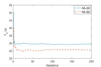
Refer to caption
Figure 4: The convergence of Algorithm 4. Here, K=4𝐾4K=4.

VIII-B Results and Discussions

VIII-B1 Effectiveness of the proposed algorithm

First, we evaluate the convergence behavior of the proposed Algorithm 4. Fig. 4 shows the effective training time Tesubscript𝑇𝑒T_{e} versus the number of iterations with D=0.5𝐷0.5D=0.5 km, K=4,τt=10formulae-sequence𝐾4subscript𝜏𝑡10K=4,\tau_{t}=10 and M={30,50}𝑀3050M=\{30,50\} for an arbitrary large-scale fading realization. It can be seen from Fig. 4 that Algorithm 4 converges in fewer than 100100100 iterations. It is also worth noting that each iteration of Algorithm 4 corresponds to solving simple convex programs (49) and (57). It is therefore expected that Algorithm 4 has a low computational complexity.

To further evaluate the effectiveness of Algorithm 4, we consider the following baseline schemes:

  • Baseline 1 (BL1): The DL powers allocated to all UEs are the same, i.e., ηmkσmk2=1/K,m,ksubscript𝜂𝑚𝑘superscriptsubscript𝜎𝑚𝑘21𝐾for-all𝑚𝑘\eta_{mk}\sigma_{mk}^{2}=1/K,\forall m,k. The transmitted UL power of each UE is maximum, i.e., ζk=1,ksubscript𝜁𝑘1for-all𝑘\zeta_{k}=1,\forall k. The local accuracy is fixed, i.e., θ=θmax+θmin2𝜃subscript𝜃subscript𝜃2\theta=\frac{\theta_{\max}+\theta_{\min}}{2} dB. The data rates and processing frequencies of UEs are then optimized.

  • Baseline 2 (BL2): This baseline is similar to BL1 except that θ𝜃\theta is optimized by a slightly modified version of Algorithm 4 (without using Algorithm 3).

  • Baseline 3 (BL3): This baseline is similar to BL1 except that the transmitted DL and UL powers are optimized by Algorithm 3. Here, the effective training time of FL is the averaged time of one FL process taken over the large-scale fading realizations.

Figs. 6 and 6 compare the effective training time Tesubscript𝑇𝑒T_{e} by the considered schemes. As seen, Algorithm 4 gives the best performance. In particular, compared to BL1, the time reduction by Algorithm 4 is up to 55%percent5555\% with M=50𝑀50M=50, K=8𝐾8K=8. Note that BL2 and BL3 also perform much better than BL1, e.g., up to 29%percent2929\% in term of time reduction with M=50,K=2formulae-sequence𝑀50𝐾2M=50,K=2 and 38%percent3838\% with M=50,K=8formulae-sequence𝑀50𝐾8M=50,K=8, respectively. Even so, Algorithm 4 still provides substantial time reductions over BL2 and BL3, e.g., up to 49%percent4949\% with M=50,K=8formulae-sequence𝑀50𝐾8M=50,K=8 and 43%percent4343\% with M=90,K=4formulae-sequence𝑀90𝐾4M=90,K=4, respectively.

The figures not only show the importance of optimizing transmit power or local accuracy, but also demonstrate the noticeable advantage of joint optimization design. Moreover, thanks to the array gain, the data rates of UEs increase when the number of APs increases. This leads to the decrease in the effective training time as shown in Fig. 6. It can also be observed from Fig. 6 that a dramatic increase in the training time when the number of UEs increases. This is because the mutual interference and pilot contamination become stronger for a larger number of UEs.
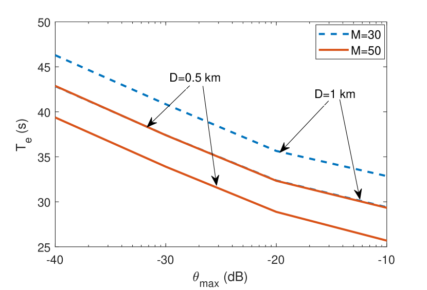
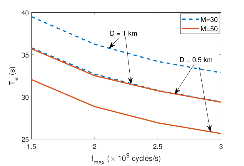
Refer to caption
Figure 5: Comparison among the baselines and Algorithm 4. Here, K=4𝐾4K=4.
Refer to caption
Figure 6: Comparison among the baselines and Algorithm 4. Here, M=50𝑀50M=50.
Refer to caption
Figure 7: Impact of the local accuracy on the effective training time. Here, K=4𝐾4K=4.
Refer to caption
Figure 8: Impact of UE’s processing frequency on the effective training time. Here, K=4𝐾4K=4.

VIII-B2 Impact of key system parameters on the effective training time

The impact of the local accuracy on the effective training time is shown in Fig. 8. Decreasing the threshold θmaxsubscript𝜃\theta_{\max} leads to a dramatic increase in the effective training time, e.g., by up to 33%percent3333\% with θmax=40subscript𝜃40\theta_{\max}=-40 dB in comparison to that with θmax=10subscript𝜃10\theta_{\max}=-10. This is reasonable because at a lower value of θ𝜃\theta, more iterations are required for local training. To keep the energy consumption of UEs below Emaxsubscript𝐸E_{\max}, the UEs’ processing frequencies become smaller. This leads to an increase in the time required to compute the local training updates.

Fig. 8 shows the impact of UE’s processing frequency on the effective training time. As seen, the effective training time increases when the threshold fmaxsubscript𝑓f_{\max} decreases. In particular, the increase is by up to 19%percent1919\% with fmax=1.5×10⁹subscript𝑓1.5superscript109f_{\max}=1.5\times 10^{9} cycles/s in comparison to that with fmax=3×10⁹subscript𝑓3superscript109f_{\max}=3\times 10^{9} cycles/s. This is because at a lower value of UEs’ processing frequency, it requires more time to compute the local training updates.

In Fig. 10, the impact of UE’s energy consumption limit Emaxsubscript𝐸E_{\max} on the effective training time is revealed. Here, decreasing Emaxsubscript𝐸E_{\max} leads to an increase in the effective time. Specifically, the increase is by up to 9.4%percent9.49.4\% with Emax=2subscript𝐸2E_{\max}=2 J, D=1𝐷1D=1 km in comparison to that with Emax=15subscript𝐸15E_{\max}=15 J, D=1𝐷1D=1 km. This is reasonable because at a low value of Emaxsubscript𝐸E_{\max}, the effective time may not approach the optimal value due to a smaller feasible region of the optimization problem (29). We note that in the case of deep fading, the achievable rates of UEs could be small. This may lead to an infeasible problem because the constraint (29b) on the energy consumed at each UE may be violated. However, it should be also emphasized that a cell-free massive MIMO network has many antennas distributed over a potentially large coverage area. As very high small-scale and macro diversity gains can be achieved, the probability of simultaneously experiencing deep fading for all links would be very small. The problem is therefore likely feasible and our proposed solution would apply.
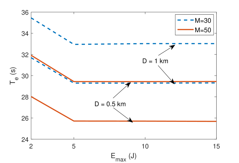
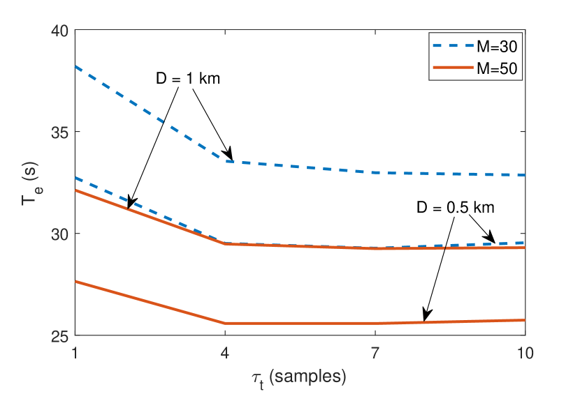
Refer to caption
Figure 9: Impact of UE’s energy consumption limit Emaxsubscript𝐸E_{\max} on the effective training time. Here, K=4𝐾4K=4.
Refer to caption
Figure 10: Impact of the length of UL pilots on the effective training time. Here, K=4𝐾4K=4.

Fig. 10 focuses on the impact of the length of UL pilots on the effective training time. It is clear that too small and too large values of τtsubscript𝜏𝑡\tau_{t} both increase the effective time. Specially, the effective time increases up to 10%percent1010\% and 1%percent11\% with τt=1subscript𝜏𝑡1\tau_{t}=1 and τt=13subscript𝜏𝑡13\tau_{t}=13 in comparison to that with τt=7subscript𝜏𝑡7\tau_{t}=7, respectively. This is reasonable because at a large value of τtsubscript𝜏𝑡\tau_{t}, the factor of TcτtTcsubscript𝑇𝑐subscript𝜏𝑡subscript𝑇𝑐\frac{T_{c}-\tau_{t}}{T_{c}} makes the data rate decrease and the transmission time grows. In contrast, at a small value of τtsubscript𝜏𝑡\tau_{t}, the network suffers more from the pilot contamination, the data rates drop and the training update transmission time increases.

VIII-B3 Cell-free massive MIMO vs. Cell-free TDMA massive MIMO

Fig. 12 compares the cell-free massive MIMO system with the cell-free TDMA massive MIMO system. Since the pilot sequences of UEs in the latter are pairwisely orthogonal in the time domain, we choose orthogonal pilot sequences for the former, i.e., 𝝋H𝝋k=0,𝒦kformulae-sequencesuperscriptsubscript𝝋𝐻subscript𝝋𝑘0for-all𝒦𝑘\operatorname{\boldsymbol{\varphi}}_{\ell}^{H}\operatorname{\boldsymbol{\varphi}}_{k}=0,\forall\ell\in\operatorname{\mathcal{K}}\setminus k, for a fair comparison. The training durations are then the same for both systems. We also choose ρ~t=Kρtsubscript~𝜌𝑡𝐾subscript𝜌𝑡\widetilde{\rho}_{t}=K\rho_{t} for the amount of energy consumed at the “UL channel estimation” time blocks of the two networks to be the same, and τt=Ksubscript𝜏𝑡𝐾\tau_{t}=K so that the powers of channel estimate, i.e., σmk2,m,ksuperscriptsubscript𝜎𝑚𝑘2for-all𝑚𝑘\sigma_{mk}^{2},\forall m,k, are the same in the two networks. From Fig. 12, a significant time reduction (e.g., of up to 94%percent9494\% with K=8𝐾8K=8) is achieved by the CFmMIMO compared with the cell-free TDMA massive MIMO. This result is expected because in the former, the factor of (1/K)1𝐾(1/K) is imposed on the data rates and the training updates are transmitted sequentially. For a large number of UEs, the data rate is significantly small, and as a result, the training update transmission requires a substantially long time.
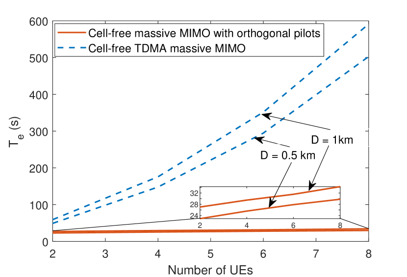
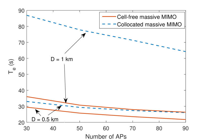
Refer to caption
Figure 11: Comparison between CFmMIMO with orthogonal pilots and cell-free TDMA massive MIMO. Here, M=50𝑀50M=50.
Refer to caption
Figure 12: Comparison between CFmMIMO and collocated massive MIMO. Here, K=4𝐾4K=4.

VIII-B4 Cell-free massive MIMO vs. Collocated massive MIMO

Finally, we compare the effective training time in CFmMIMO with that in collocated massive MIMO. Fig. 12 shows that the former significantly outperform the latter, e.g., the time reduction is by up to 57%percent5757\% with M=30𝑀30M=30 and D=1𝐷1D=1 km. This observation is as expected because CFmMIMO distributes antennas over their coverage area; and as such, their performance suffers less from the UEs with unfavorable links than that of collocated massive MIMO. Higher data rates and a lower training time then follow.

IX Conclusion

In this paper, we have proposed using CFmMIMO networks to support FL in a wireless environment. We designed a general scheme in which any algorithm and beamforming/filtering approach can be further developed to optimize the performance of any FL framework. Specially here, each iteration of the FL optimization algorithms or the FL process happens in one large-scale coherence time. Targeting training time minimization for the FL framework [21] as example, we jointly design local accuracy, transmit power, data rate, and UE’s processing frequency under the practical requirements on the UE’s energy consumption limit and maximum transmit powers at the APs and UEs. A mixed timescale stochastic nonconvex optimization problem has been formulated with the objective of minimizing the training time of one FL process. Based on the general online successive convex approximation framework, we have developed a new algorithm to successfully solve the formulated problem. We have proved that the proposed algorithm converges to the neighborhood of stationary points of the optimization problem. For given parameter settings, numerical results show that our joint optimization design significantly reduces the training time of FL over the baselines under comparison. They have also confirmed that CFmMIMO offers the lowest training time when compared with cell-free TDMA massive MIMO and collocated massive MIMO.

References

  • [1] K. B. Letaief, W. Chen, Y. Shi, J. Zhang, and Y. A. Zhang, “The roadmap to 6G: AI empowered wireless networks,” IEEE Commun. Mag., vol. 57, no. 8, pp. 84–90, Aug. 2019.
  • [2] F. D. Calabrese, L. Wang, E. Ghadimi, G. Peters, L. Hanzo, and P. Soldati, “Learning radio resource management in RANs: Framework, opportunities, and challenges,” IEEE Commun. Mag., vol. 56, no. 9, pp. 138–145, Sep. 2018.
  • [3] J. Dong, M. Noreikis, Y. Xiao, and A. Ylä-Jääski, “Vinav: A vision-based indoor navigation system for smartphones,” IEEE Trans. Mobile Comput., vol. 18, no. 6, pp. 1461–1475, Jun. 2019.
  • [4] Qualcomm, “We are making on-device AI ubiquitous,” https://www.qualcomm.com/news/onq/2017/08/16/we-are-making-device-ai-ubiquitous, 2017.
  • [5] Gartner, “Gartner highlights 10 uses for AI-powered smartphones,” https://www.gartner.com/en/newsroom/press-releases/2018-03-20-gartner-highlights-10-uses-for-ai-powered-smartphones, 2018.
  • [6] G. Zhu, D. Liu, Y. Du, C. You, J. Zhang, and K. Huang, “Towards an intelligent edge: Wireless communication meets machine learning,” 2018. [Online]. Available: http://arxiv.org/abs/1809.00343
  • [7] H. A. Alameddine, S. Sharafeddine, S. Sebbah, S. Ayoubi, and C. Assi, “Dynamic task offloading and scheduling for low-latency iot services in multi-access edge computing,” IEEE J. Sel. Areas Commun,, vol. 37, no. 3, pp. 668–682, Mar. 2019.
  • [8] M. Chen and Y. Hao, “Task offloading for mobile edge computing in software defined ultra-dense network,” IEEE J. Sel. Areas Commun., vol. 36, no. 3, pp. 587–597, Mar. 2018.
  • [9] T. Li, A. K. Sahu, A. Talwalkar, and V. Smith, “Federated learning: Challenges, methods, and future directions,” 2019. [Online]. Available: https://arxiv.org/abs/1908.07873
  • [10] N. H. Tran, W. Bao, A. Zomaya, N. Minh N.H., and C. S. Hong, “Federated learning over wireless networks: Optimization model design and analysis,” in Proc. IEEE Conf. Comput. Commun. (INFOCOM), Apr. 2019, pp. 1387–1395.
  • [11] B. McMahan, E. Moore, D. Ramage, S. Hampson, and B. A. y Arcas, “Communication-Efficient Learning of Deep Networks from Decentralized Data,” in Proc. Int. Conf. Artificial Intell. Statist., vol. 54, Fort Lauderdale, FL, USA, Apr. 2017, pp. 1273–1282.
  • [12] A. Hard, K. Rao, R. Mathews, F. Beaufays, S. Augenstein, H. Eichner, C. Kiddon, and D. Ramage, “Federated learning for mobile keyboard prediction,” 2018. [Online]. Available: http://arxiv.org/abs/1811.03604
  • [13] F. Sattler, S. Wiedemann, K. Müller, and W. Samek, “Robust and communication-efficient federated learning from Non-IID data,” 2019. [Online]. Available: http://arxiv.org/abs/1903.02891
  • [14] J. Kang, Z. Xiong, D. Niyato, H. Yu, Y. Liang, and D. I. Kim, “Incentive design for efficient federated learning in mobile networks: A contract theory approach,” 2019. [Online]. Available: http://arxiv.org/abs/1905.07479
  • [15] S. Wang, T. Tuor, T. Salonidis, K. K. Leung, C. Makaya, T. He, and K. Chan, “Adaptive federated learning in resource constrained edge computing systems,” IEEE J. Sel. Areas Commun., vol. 37, no. 6, pp. 1205–1221, Jun. 2019.
  • [16] K. Yang, T. Jiang, Y. Shi, and Z. Ding, “Federated learning via over-the-air computation,” IEEE Trans. Wireless Commun., vol. 19, no. 3, pp. 2022–2035, 2020.
  • [17] M. Chen, Z. Yang, W. Saad, C. Yin, H. V. Poor, and S. Cui, “A joint learning and communications framework for federated learning over wireless networks,” 2019. [Online]. Available: https://arxiv.org/abs/1909.07972
  • [18] J. Zhang, S. Chen, Y. Lin, J. Zheng, B. Ai, and L. Hanzo, “Cell-free massive MIMO: A new next-generation paradigm,” IEEE Access, vol. 7, pp. 99 878–99 888, 2019.
  • [19] H. Q. Ngo, A. Ashikhmin, H. Yang, E. G. Larsson, and T. L. Marzetta, “Cell-free massive MIMO versus small cells,” IEEE Trans. Wireless Commun., vol. 16, no. 3, pp. 1834–1850, Mar. 2017.
  • [20] T. L. Marzetta, E. G. Larsson, H. Yang, and H. Q. Ngo, Fundamentals of Massive MIMO.   Cambridge University Press, 2016.
  • [21] C. Ma, J. Konec̆ný, M. Jaggi, V. Smith, M. I. Jordan, P. Richtárik, and M. Takáč, “Distributed optimization with arbitrary local solvers,” Optimization Methods Software, vol. 32, no. 4, pp. 813–848, Jul. 2017.
  • [22] A. Liu, V. K. N. Lau, and M. Zhao, “Online successive convex approximation for two-stage stochastic nonconvex optimization,” IEEE Trans. Signal Process., vol. 66, no. 22, pp. 5941–5955, Nov. 2018.
  • [23] J. Ahn, O. Simeone, and J. Kang, “Wireless federated distillation for distributed edge learning with heterogeneous data,” 2019. [Online]. Available: http://arxiv.org/abs/1907.02745
  • [24] M. Mohri, G. Sivek, and A. T. Suresh, “Agnostic federated learning,” 2019. [Online]. Available: http://arxiv.org/abs/1902.00146
  • [25] H. Zhu and Y. Jin, “Multi-objective evolutionary federated learning,” 2018. [Online]. Available: http://arxiv.org/abs/1812.07478
  • [26] J. Konec̆ný, Z. Qu, and P. Richtárik, “Semi-stochastic coordinate descent,” Optimization Methods and Software, vol. 32, no. 5, pp. 993–1005, 2017.
  • [27] M. Jaggi, V. Smith, M. Takáč, J. Terhorst, S. Krishnan, T. Hofmann, and M. I. Jordan, “Communication-efficient distributed dual coordinate ascent,” in Proc. 27th Int. Conf. Neural Inform. Process. Syst. (NIPS), vol. 2, 2014, pp. 3068–3076.
  • [28] E. Björnson, J. Hoydis, and L. Sanguinetti, “Massive MIMO networks: Spectral, energy, and hardware efficiency,” Found. Trends. Signal Process., vol. 11, no. 3-4, pp. 154–655, 2017.
  • [29] S. M. Kay, Fundamentals of Statistical Signal Processing: Estimation Theory.   Upper Saddle River, NJ, USA: Prentice-Hall, Inc., 1993.
  • [30] A. P. Miettinen and J. K. Nurminen, “Energy efficiency of mobile clients in cloud computing,” in Proc. 2nd USENIX Conf. HotCloud, 2010.
  • [31] S. Boyd and L. Vandenberghe, Convex Optimization.   New York, NY: Cambridge University Press, 2004.
  • [32] T. T. Vu, D. T. Ngo, M. N. Dao, S. Durrani, D. H. N. Nguyen, and R. H. Middleton, “Energy efficiency maximization for downlink cloud radio access networks with data sharing and data compression,” IEEE Trans. Wireless Commun., vol. 17, no. 8, pp. 4955–4970, Aug. 2018.
  • [33] V. D. Nguyen, T. Q. Duong, H. D. Tuan, O. S. Shin, and H. V. Poor, “Spectral and energy efficiencies in full-duplex wireless information and power transfer,” IEEE Trans. Commun., vol. 65, no. 5, pp. 2220–2233, May 2017.
  • [34] B. R. Marks and G. P. Wright, “A general inner approximation algorithm for nonconvex mathematical programs,” Operations Research, vol. 26, no. 4, pp. 681–683, 1978.
  • [35] H. Q. Ngo, L. Tran, T. Q. Duong, M. Matthaiou, and E. G. Larsson, “On the total energy efficiency of cell-free massive MIMO,” IEEE Trans. Green Commun. Netw., vol. 2, no. 1, pp. 25–39, Mar. 2018.
Tung Thanh Vu (S’17) received the B.Sc. degree (Hons.) in telecommunications and networking from Ho Chi Minh City University of Science in 2012 and the M.Sc. degree (Hons.) in telecommunications engineering from Ho Chi Minh City University of Technology in 2016. He is currently a PhD candidate in the School of Electrical Engineering and Computing, The University of Newcastle, Australia. His current research interests include optimization designs and machine learning for cell-free massive MIMO and cloud radio access networks.
Duy Trong Ngo (S’08-M’15) received the B.Eng. degree (Hons.) in telecommunication engineering from The University of New South Wales, Australia, in 2007, the M.Sc. degree in electrical engineering (communication) from the University of Alberta, Canada, in 2009, and the Ph.D. degree in electrical engineering from McGill University, Canada, in 2013. He is a Senior Lecturer with the School of Electrical Engineering and Computing, The University of Newcastle, Australia, where he is currently involved in the research effort of design and optimization for 5G and beyond wireless communications networks. His current research interests include cloud radio access networks, multi-access edge computing, and vehicle-to-everything (V2X) communications for intelligent transportation systems.
Nguyen H. Tran (S’10-M’11-SM’18) received BS and Ph.D degrees, from HCMC University of Technology and Kyung Hee University, in electrical and computer engineering, in 2005 and 2011, respectively. He was an Assistant Professor with Department of Computer Science and Engineering, Kyung Hee University, from 2012 to 2017. Since 2018, he has been with the School of Computer Science, The University of Sydney, where he is currently a Senior Lecturer. His research interests include distributed computing, machine learning, and networking. He received the best KHU thesis award in engineering in 2011 and several best paper awards, including IEEE ICC 2016, APNOMS 2016, IEEE ICCS 2016, and ACM MSWiM 2019. He receives the Korea NRF Funding for Basic Science and Research 2016-2023 and ARC Discovery Project 2020-2023. He has been the Editor of IEEE Transactions on Green Communications and Networking since 2016.
Hien Quoc Ngo is currently a Lecturer at Queen’s University Belfast, UK. His main research interests include massive (large-scale) MIMO systems, cellfree massive MIMO, physical layer security, and cooperative communications. He has co-authored many research papers in wireless communications and co-authored the Cambridge University Press textbook Fundamentals of Massive MIMO (2016). He received the IEEE ComSoc Stephen O. Rice Prize in Communications Theory in 2015, the IEEE ComSoc Leonard G. Abraham Prize in 2017, and the Best Ph.D. Award from EURASIP in 2018.
Minh Ngoc Dao received the Ph.D. degree in applied mathematics from the University of Toulouse, France, in 2014. He was a Postdoctoral Fellow with The University of British Columbia, Canada, from 2014 to 2016, and a Research Associate with The University of Newcastle, Australia, from 2016 to 2019. He is currently a Research Associate with The University of New South Wales, Australia. His research interests include nonlinear optimization, nonsmooth analysis, control theory, signal processing, and machine learning. In 2017, he received the Annual Best Paper Award from the Journal of Global Optimization.
Richard H. Middleton (SM’86–-F’99) completed his Ph.D. (1987) from the University of Newcastle, Australia. He was a Research Professor at the Hamilton Institute, The National University of Ireland, Maynooth from May 2007 till 2011 and is currently Professor at the University of Newcastle and Head of the School of Electrical Engineering and Computing. He has served as Program Chair (CDC 2006), co-general chair (CDC 2017) CSS Vice President Membership Activities, and Vice President Conference Activities. In 2011, he was President of the IEEE Control Systems Society. He is a Fellow of IEEE and of IFAC, and his research interests include a broad range of Control Systems Theory and Applications, including Communications Systems, control of distributed systems and Systems Biology.