Data-Driven Robust Stabilization with Robust Domain of Attraction Estimate for Nonlinear Discrete-Time Systems

Yongqiang Li yqli@zjut.edu.cn    Chaolun Lu 2111703050@zjut.edu.cn    Zhongsheng Hou zshou@qdu.edu.cn    Yuanjing Feng fyjing@zjut.edu.cn College of Information Engineering, Zhejiang University of Technology, Hangzhou, China School of Automation, Qingdao University, Qingdao, China
Abstract

Nonlinear robust control is pursued by overcoming the drawback of linear robust control that it ignores available information about existing nonlinearities and the resulting controllers may be too conservative, especially when the nonlinearities are significant. However, most existing nonlinear robust control approaches just consider the affine nonlinear nominal model and thereby ignore available information about existing non-affine nonlinearities. When the general nonlinear nominal model is considered, the robust domain of attraction (RDOA) of closed-loops requires extensive investigation because it is hard to achieve the global stabilization. In this paper, we propose a new nonlinear robust control method based on Lyapunov function to stabilize a discrete-time uncertain system and to estimate the RDOA of closed-loops. First, a sufficient condition for robust stabilization of all plants in a plant set and estimation of the RDOA of all closed-loops is proposed. Then, to tackle the non-affine nonlinearities, a data-driven method of estimating the robust negative-definite domains (RNDD) is presented, and based on it the estimation of the RDOA of closed-loops and the resulting controller design are also given.

keywords:
Data-based control, Robust control of nonlinear systems, Asymptotic stabilization, Domain of attraction
thanks: This paper was not presented at any IFAC meeting. Corresponding author Y. Feng. Tel. +086-13567173448.

, , , ,

1 Introduction

Robust control theory is one of the most important branches of the modern control theory, due to its ability of dealing with the uncertainty describing how the ”true” plant might differ from the nominal model. Most of robust control theory is linear (assume that the nominal model is linear) [12, 10, 2]. A disadvantage of linear robust control is that it ignores available information about existing nonlinearities, and the resulting controllers may be too conservative (especially when the nonlinearities are significant). A natural attempt to overcome this drawback is to allow the nominal model to be nonlinear and thereby pursue nonlinear robust control design [5].

Popular frameworks for robust nonlinear control include the Lyapunov min-max approach [4], the nonlinear H approach [1, 14], the input-to-state stability approach [13] and the robust backstepping approach [5]. In these approaches, the nonlinear nominal model is affine with respect to the control, namely, affine nonlinear. Similar to the linear robust control, these approaches ignore available information about existing non-affine nonlinearities. A natural solution is to allow the nominal model to be non-affine nonlinear.

For non-affine nonlinear system without uncertainty, due to the difficulty to achieve the global stabilization, the domain of attraction (DOA) of the closed-loop, an invariant set characterizing asymptotically stabilizable area around the equilibrium, requires extensive investigation [3, 6, 9]. With the same reason, when the nominal model in robust control is non-affine nonlinear, the RDOA of the closed-loops also requires investigation under certain conditions. This issue is so difficult such that no result is published for robust controller design up to our knowledge. For system analysis, [7] proposes a method of estimating the RDOA for continuous-time autonomous systems under uncertainties.

In this paper, we propose a new robust nonlinear control method based on Lyapunov function to stabilize a discrete-time uncertain system and estimate the RDOA of closed-loops. The uncertain system is described by a function set characterized by the nominal model and the corresponding modeling error bound. First, a sufficient condition for robust stabilization of all plants in the function set and estimation of the RDOA of all closed-loops is proposed. It is shown that if a state feedback controller belongs to the RNDD in the state-control space (RNDD-SC), in which all points make the difference of a given Lyapunov function to be negative-definite for all plants, it can asymptotically stabilize all plants. Meanwhile, any level-set of the Lyapunov function belonging to the RNDD in the state space (RNDD-S) can be an estimate of the RDOA of all closed-loops. Hence, if the RNDD-SC can be obtained, it is easy to find a robust controller and an estimate of the RDOA of closed-loops. However, due to nonlinearities, it is hard to obtain analytic solution of the RNDD-SC. Then, a data-driven method of estimating the RNDD-SC is proposed. The idea is much simple. The state-control space is partitioned into disjoint cells. The estimate of the RNDD-SC consists of cells in which all data points satisfying specific conditions. We would like stress that the present paper considers a given Lyapunov function and addresses the problem of robust stabilization and estimation of RDOA from it. The problem of finding good Lyapunov functions is not in the scope of this paper.

The rest of this paper is organized as follows. In Section 2, the control problem is formulated. In Section 3, sufficient conditions for robust stabilization and estimation of the RDOA of all closed-loops are proposed. In Section 4, a data-driven robust stabilization with the RDOA estimation is derived. Finally, the conclusion is drawn in Section 5.

Notation: For xn𝑥superscript𝑛x\in\mathbb{R}^{n} and um𝑢superscript𝑚u\in\mathbb{R}^{m}, (x;u)𝑥𝑢(x;u) represents a new vector in n+msuperscript𝑛𝑚\mathbb{R}^{n+m}. For x1,x2nsubscript𝑥1subscript𝑥2superscript𝑛x_{1},x_{2}\in\mathbb{R}^{n}, x1x2subscript𝑥1subscript𝑥2x_{1}\leq x_{2} means x1subscript𝑥1x_{1} is less than or equal to x2subscript𝑥2x_{2} element by element.

2 Problem formulation

Consider the plant set

𝔉={f:n×mn|f(0,0)=0,\displaystyle\!\!\mathfrak{F}=\Big{\{}f:\mathbb{R}^{n}\!\times\!\mathbb{R}^{m}\!\to\!\mathbb{R}^{n}\Big{|}f(0,0)=0,
f^(x,u)δ(x,u)f(x,u)f^(x,u)+δ(x,u)},\displaystyle\quad\hat{f}(x,u)-\delta(x,u)\leq f(x,u)\leq\hat{f}(x,u)+\delta(x,u)\Big{\}}, (1)

where nominal model f^:n×mn:^𝑓superscript𝑛superscript𝑚superscript𝑛\hat{f}:\mathbb{R}^{n}\times\mathbb{R}^{m}\to\mathbb{R}^{n} and modeling error bound δ:n×m+n:𝛿superscript𝑛superscript𝑚subscriptsuperscript𝑛\delta:\mathbb{R}^{n}\times\mathbb{R}^{m}\to\mathbb{R}^{n}_{+} are continuous, satisfying f^(0,0)=0^𝑓000\hat{f}(0,0)=0 and δ(0,0)=0𝛿000\delta(0,0)=0, xn𝑥superscript𝑛x\in\mathbb{R}^{n} is state and um𝑢superscript𝑚u\in\mathbb{R}^{m} is control input. The control objective is to find a robust controller μ𝜇\mu and an estimate of the RDOA such that, f𝔉for-all𝑓𝔉\forall f\in\mathfrak{F}, the closed-loop x(k+1)=f(x(k),μ(x(k)))𝑥𝑘1𝑓𝑥𝑘𝜇𝑥𝑘x(k+1)=f(x(k),\mu(x(k))) is asymptotically stable at the origin for all initial state in the estimate of the RDOA.

Remark 1.

The nominal model error bound is described by a function rather than a constant. This can take advantage of available information about existing nonlinearities of the nominal model error bound and avoid that the resulting controllers and estimates of the RDOA may be too conservative. There are data-driven modeling methods which can give such error bound, e.g., Gaussian processes regression [11].

3 Sufficient condition for robust stabilization with robust DOA estimate
Refer to caption
Refer to caption
Refer to caption

(a)

(b)

(c)

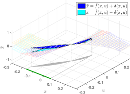
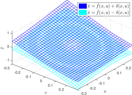
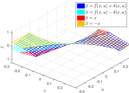
Figure 1: (a) Plant set Π𝔉subscriptΠ𝔉\Pi_{\mathfrak{F}}. (b) Negative-definite domain Π~𝔉(L)subscript~Π𝔉𝐿\tilde{\Pi}_{\mathfrak{F}}(L). (c) Robust negative-definite domains Π𝔉(L)subscriptΠ𝔉𝐿\Pi_{\mathfrak{F}}(L), 𝕎𝔉(L)subscript𝕎𝔉𝐿\mathbb{W}_{\mathfrak{F}}(L) and 𝕏𝔉(L)subscript𝕏𝔉𝐿\mathbb{X}_{\mathfrak{F}}(L).

For given nominal model f^^𝑓\hat{f} and modeling error bound δ𝛿\delta, the plant set 𝔉𝔉\mathfrak{F} defined in (1) can be alternatively described as a domain

Π𝔉={(x¯;x;u)|f^(x,u)δ(x,u)x¯f^(x,u)+δ(x,u)}subscriptΠ𝔉conditional-set¯𝑥𝑥𝑢^𝑓𝑥𝑢𝛿𝑥𝑢¯𝑥^𝑓𝑥𝑢𝛿𝑥𝑢\displaystyle\Pi_{\mathfrak{F}}\!=\!\Big{\{}(\bar{x};x;u)\Big{|}\hat{f}(x,\!u)\!-\!\delta(x,\!u)\!\leq\!\bar{x}\!\leq\!\hat{f}(x,\!u)\!+\!\delta(x,\!u)\Big{\}} (2)

in (2n+m)2𝑛𝑚(2n+m)-dimensional space, where x¯n¯𝑥superscript𝑛\bar{x}\in\mathbb{R}^{n} denotes the future state (i.e. the state at the next time step), xn𝑥superscript𝑛x\in\mathbb{R}^{n} and um𝑢superscript𝑚u\in\mathbb{R}^{m} denote the current state and control input. Considering a continuous positive-definite function L:n:𝐿superscript𝑛L:\mathbb{R}^{n}\to\mathbb{R}, we define the negative-definite domain in the state-state-control space (NDD-SSC) Π~𝔉(L)subscript~Π𝔉𝐿\tilde{\Pi}_{\mathfrak{F}}(L) as

Π~𝔉(L)={(x¯;x;u)Π𝔉|L(x¯)L(x)<0}.subscript~Π𝔉𝐿conditional-set¯𝑥𝑥𝑢subscriptΠ𝔉𝐿¯𝑥𝐿𝑥0\displaystyle\tilde{\Pi}_{\mathfrak{F}}(L)=\Big{\{}(\bar{x};x;u)\in\Pi_{\mathfrak{F}}\Big{|}L(\bar{x})-L(x)<0\Big{\}}. (3)

Although any point (x¯;x;u)Π~𝔉(L)¯𝑥𝑥𝑢subscript~Π𝔉𝐿(\bar{x};x;u)\in\tilde{\Pi}_{\mathfrak{F}}(L) makes the time difference of L𝐿L to be negative-definite (i.e., L(x¯)L(x)<0𝐿¯𝑥𝐿𝑥0L(\bar{x})-L(x)<0), Π~𝔉(L)subscript~Π𝔉𝐿\tilde{\Pi}_{\mathfrak{F}}(L) is not robust for plant set (1). Because it is not guaranteed that, for given (x;u)𝑥𝑢(x;u), f𝔉for-all𝑓𝔉\forall f\in\mathfrak{F} satisfies L(f(x,u))L(x)<0𝐿𝑓𝑥𝑢𝐿𝑥0L(f(x,u))-L(x)<0. In order to define the robust NDD-SSC (RNDD-SSC), we first define the future state set 𝕏¯𝔉(x,u)subscript¯𝕏𝔉𝑥𝑢\bar{\mathbb{X}}_{\mathfrak{F}}(x,u) for the given (x;u)𝑥𝑢(x;u) as follows.

𝕏¯𝔉(x,u)={x¯n|f^(x,u)δ(x,u)x¯f^(x,u)+δ(x,u)}.subscript¯𝕏𝔉𝑥𝑢conditional-set¯𝑥superscript𝑛^𝑓𝑥𝑢𝛿𝑥𝑢¯𝑥^𝑓𝑥𝑢𝛿𝑥𝑢\displaystyle\bar{\mathbb{X}}_{\mathfrak{F}}(x,\!u)\!=\!\Big{\{}\bar{x}\!\in\!\mathbb{R}^{n}\Big{|}\hat{f}(\!x,\!u\!)\!-\!\delta(\!x,\!u\!)\!\leq\!\bar{x}\!\leq\!\hat{f}(\!x,\!u\!)\!+\!\delta(\!x,\!u\!)\!\Big{\}}. (4)

With 𝕏¯𝔉(x,u)subscript¯𝕏𝔉𝑥𝑢\bar{\mathbb{X}}_{\mathfrak{F}}(x,u), the RNDD-SSC Π𝔉(L)subscriptΠ𝔉𝐿\Pi_{\mathfrak{F}}(L) is defined as

Π𝔉(L)={(x¯;x;u)Π~𝔉(L)|\displaystyle\!\!\Pi_{\mathfrak{F}}(L)=\Big{\{}(\bar{x};x;u)\in\tilde{\Pi}_{\mathfrak{F}}(L)\Big{|}
x¯𝕏¯𝔉(x,u),L(x¯)L(x)<0,x¯𝕏¯𝔉(x,u)}.\displaystyle\quad\forall\bar{x}^{\prime}\in\bar{\mathbb{X}}_{\mathfrak{F}}(x,u),L(\bar{x}^{\prime})-L(x)<0,\bar{x}\in\bar{\mathbb{X}}_{\mathfrak{F}}(x,u)\Big{\}}. (5)

Projecting Π𝔉(L)subscriptΠ𝔉𝐿\Pi_{\mathfrak{F}}(L) along the future state space onto the state-control space, the RNDD in the state-control space (RNDD-SC) 𝕎𝔉(L)subscript𝕎𝔉𝐿\mathbb{W}_{\mathfrak{F}}(L) is defined as

𝕎𝔉(L)={(x;u)n+m|x¯𝕏¯𝔉(x,u),L(x¯)L(x)<0}.subscript𝕎𝔉𝐿conditional-set𝑥𝑢superscript𝑛𝑚formulae-sequencefor-all¯𝑥subscript¯𝕏𝔉𝑥𝑢𝐿¯𝑥𝐿𝑥0\displaystyle\mathbb{W}\!_{\mathfrak{F}}\!(L)\!=\!\Big{\{}\!(x;\!u)\!\in\!\mathbb{R}^{n+m}\Big{|}\forall\bar{x}\!\in\!\bar{\mathbb{X}}_{\mathfrak{F}}(x,\!u),L\big{(}\!\bar{x}\!\big{)}\!-\!L(\!x\!)\!<\!0\Big{\}}.\! (6)

The RNDD-SC 𝕎𝔉(L)subscript𝕎𝔉𝐿\mathbb{W}_{\mathfrak{F}}(L) is an open set, because its boundary {(x;u)|x¯𝕏¯𝔉(x,u),L(x¯)L(x)0}\𝕎𝔉(L)\conditional-set𝑥𝑢formulae-sequencefor-all¯𝑥subscript¯𝕏𝔉𝑥𝑢𝐿¯𝑥𝐿𝑥0subscript𝕎𝔉𝐿\{(x;u)|\forall\bar{x}\in\bar{\mathbb{X}}_{\mathfrak{F}}(x,u),L(\bar{x})-L(x)\leq 0\}\backslash\mathbb{W}_{\mathfrak{F}}(L) is not its subset, where A\B={aA|aB}\𝐴𝐵conditional-set𝑎𝐴𝑎𝐵A\backslash B=\{a\in A|a\notin B\}. It is obvious that the origin (0;0)n+m00superscript𝑛𝑚(0;0)\in\mathbb{R}^{n+m} is in the boundary of 𝕎𝔉(L)subscript𝕎𝔉𝐿\mathbb{W}_{\mathfrak{F}}(L). Due to 𝕏¯𝔉(0,0)={0}subscript¯𝕏𝔉000\bar{\mathbb{X}}_{\mathfrak{F}}(0,0)=\{0\} and the continuity of f^,δ^𝑓𝛿\hat{f},\delta and L𝐿L, there is a subset of the neighborhood of the origin (0;0)00(0;0) contained by 𝕎𝔉(L)subscript𝕎𝔉𝐿\mathbb{W}_{\mathfrak{F}}(L) although the origin (0;0)00(0;0) is not contained by 𝕎𝔉(L)subscript𝕎𝔉𝐿\mathbb{W}_{\mathfrak{F}}(L). Projecting 𝕎𝔉(L)subscript𝕎𝔉𝐿\mathbb{W}_{\mathfrak{F}}(L) along the control space onto the state space, the RNDD in the state space (RNDD-S) 𝕏𝔉(L)subscript𝕏𝔉𝐿\mathbb{X}_{\mathfrak{F}}(L) is defined as

𝕏𝔉(L)={xn|um,(x;u)𝕎𝔉(L)}.subscript𝕏𝔉𝐿conditional-set𝑥superscript𝑛formulae-sequence𝑢superscript𝑚𝑥𝑢subscript𝕎𝔉𝐿\displaystyle\mathbb{X}_{\mathfrak{F}}(L)=\Big{\{}x\in\mathbb{R}^{n}\Big{|}\exists u\in\mathbb{R}^{m},(x;u)\in\mathbb{W}_{\mathfrak{F}}(L)\Big{\}}. (7)

The RNDD-S 𝕏𝔉(L)subscript𝕏𝔉𝐿\mathbb{X}_{\mathfrak{F}}(L) does not contain the origin 0n0superscript𝑛0\in\mathbb{R}^{n} but contains a neighborhood of the origin. Examples of plant set Π𝔉subscriptΠ𝔉\Pi_{\mathfrak{F}}, NDD-SSC Π~𝔉(L)subscript~Π𝔉𝐿\tilde{\Pi}_{\mathfrak{F}}(L), RNDD-SSC Π𝔉(L)subscriptΠ𝔉𝐿\Pi_{\mathfrak{F}}(L), RNDD-SC 𝕎𝔉(L)subscript𝕎𝔉𝐿\mathbb{W}_{\mathfrak{F}}(L) and RNDD-S 𝕏𝔉(L)subscript𝕏𝔉𝐿\mathbb{X}_{\mathfrak{F}}(L) are given in Example 2.

Example 2.

Consider the nominal model f^(x,u)=sin(2x)xu0.2xu2+u^𝑓𝑥𝑢2𝑥𝑥𝑢0.2𝑥superscript𝑢2𝑢\hat{f}(x,u)=-\sin(2x)-xu-0.2x-u^{2}+u and the model error bound δ=1exp(2(x2+u2))𝛿12superscript𝑥2superscript𝑢2\delta=1-\exp\left(-2(x^{2}+u^{2})\right), where x𝑥x\in\mathbb{R} and u𝑢u\in\mathbb{R}.The plant set Π𝔉3subscriptΠ𝔉superscript3\Pi_{\mathfrak{F}}\subset\mathbb{R}^{3} defined in (2) is shown in Figure 1 (a). Considering the positive-definite function L(x)=x2𝐿𝑥superscript𝑥2L(x)=x^{2}, the NDD-SSC Π~𝔉(L)3subscript~Π𝔉𝐿superscript3\tilde{\Pi}_{\mathfrak{F}}(L)\subset\mathbb{R}^{3} defined in (3) is shown in Figure 1 (b). Any (x¯;x;u)3¯𝑥𝑥𝑢superscript3(\bar{x};x;u)\in\mathbb{R}^{3} between the surfaces x¯=x¯𝑥𝑥\bar{x}=x and x¯=x¯𝑥𝑥\bar{x}=-x satisfies x¯2x2<0superscript¯𝑥2superscript𝑥20\bar{x}^{2}-x^{2}<0. Hence, boundaries of Π~𝔉(L)3subscript~Π𝔉𝐿superscript3\tilde{\Pi}_{\mathfrak{F}}(L)\subset\mathbb{R}^{3} consist of four surfaces: x¯=f^(x,u)+δ(x,u),x¯=f^(x,u)δ(x,u),x¯=xformulae-sequence¯𝑥^𝑓𝑥𝑢𝛿𝑥𝑢formulae-sequence¯𝑥^𝑓𝑥𝑢𝛿𝑥𝑢¯𝑥𝑥\bar{x}=\hat{f}(x,u)+\delta(x,u),\bar{x}=\hat{f}(x,u)-\delta(x,u),\bar{x}=x and x¯=x¯𝑥𝑥\bar{x}=-x.

The RNDD-SSC Π𝔉(L)3subscriptΠ𝔉𝐿superscript3\Pi_{\mathfrak{F}}(L)\subset\mathbb{R}^{3} defined in (5) is shown in Figure 1 (c) denoted by the domain between the blue patch in the surface x¯=f^(x,u)+δ(x,u)¯𝑥^𝑓𝑥𝑢𝛿𝑥𝑢\bar{x}=\hat{f}(x,u)+\delta(x,u) and the cyan patch in the surface x¯=f^(x,u)δ(x,u)¯𝑥^𝑓𝑥𝑢𝛿𝑥𝑢\bar{x}=\hat{f}(x,u)-\delta(x,u). It should be noted that the boundary of the blue patch is identical with the one of the cyan patch in the state-control space. The RNDD-SC 𝕎𝔉(L)2subscript𝕎𝔉𝐿superscript2\mathbb{W}_{\mathfrak{F}}(L)\subset\mathbb{R}^{2} defined in (6) is shown in Figure 1(c) denoted by the gray region in (x(x-u)u)-plane. The RNDD-S 𝕏𝔉(L)subscript𝕏𝔉𝐿\mathbb{X}_{\mathfrak{F}}(L)\in\mathbb{R} is shown in Figure 1 (c) denoted by the green line segment in the x𝑥x-axis.

From (6), it is straightforward that, if (x(k);u(k))𝕎𝔉(L)𝑥𝑘𝑢𝑘subscript𝕎𝔉𝐿(x(k);u(k))\in\mathbb{W}_{\mathfrak{F}}(L), then, f𝔉,L(f(x(k),u(k)))L(x(k))<0formulae-sequencefor-all𝑓𝔉𝐿𝑓𝑥𝑘𝑢𝑘𝐿𝑥𝑘0\forall f\in\mathfrak{F},L(f(x(k),u(k)))-L(x(k))<0. Based on this and (7), one may concludes that closed-loops of all plants in 𝔉𝔉\mathfrak{F} are asymptotically stable for any initial state in 𝕏𝔉(L)subscript𝕏𝔉𝐿\mathbb{X}_{\mathfrak{F}}(L) if the state feedback controller belongs to 𝕎𝔉(L)subscript𝕎𝔉𝐿\mathbb{W}_{\mathfrak{F}}(L). Unfortunately, this conclusion is wrong. Because it can not be guaranteed that the future state is still in 𝕏𝔉(L)subscript𝕏𝔉𝐿\mathbb{X}_{\mathfrak{F}}(L) at the next time step. Once, the future state is outside of 𝕏𝔉(L)subscript𝕏𝔉𝐿\mathbb{X}_{\mathfrak{F}}(L), the condition that the difference of L𝐿L is negative-definite is no longer satisfied. To solve this problem, it is needed to find an invariant subset of 𝕏𝔉(L)subscript𝕏𝔉𝐿\mathbb{X}_{\mathfrak{F}}(L) as the estimate of closed-loops’ DOA. Level-set 𝕏ls(L,α)subscript𝕏ls𝐿𝛼\mathbb{X}_{\mathrm{ls}}(L,\alpha) of positive-definite function L𝐿L with constant α>0𝛼0\alpha>0 is just an invariant set, which has the property that if the current state is in 𝕏ls(L,α)subscript𝕏ls𝐿𝛼\mathbb{X}_{\mathrm{ls}}(L,\alpha), then the next time step state is also in 𝕏ls(L,α)subscript𝕏ls𝐿𝛼\mathbb{X}_{\mathrm{ls}}(L,\alpha). Hence, any level-set 𝕏ls(L,α)𝕏𝔉(L)subscript𝕏ls𝐿𝛼subscript𝕏𝔉𝐿\mathbb{X}_{\mathrm{ls}}(L,\alpha)\subset\mathbb{X}_{\mathfrak{F}}(L) can be an estimate of closed-loops’ DOA. This idea is summarized in Theorem 3.

Theorem 3.

For plant set (1), if a positive-definite function L:n:𝐿superscript𝑛L:\mathbb{R}^{n}\to\mathbb{R}, a constant α+𝛼subscript\alpha\in\mathbb{R}_{+} and a state feedback controller μ:nm:𝜇superscript𝑛superscript𝑚\mu:\mathbb{R}^{n}\to\mathbb{R}^{m} exist such that

μ(0)=0,(x;μ(x))𝕎𝔉(L),x𝕏𝔉(L),formulae-sequence𝜇00formulae-sequence𝑥𝜇𝑥subscript𝕎𝔉𝐿for-all𝑥subscript𝕏𝔉𝐿\displaystyle\!\!\mu(0)=0,(x;\mu(x))\in\mathbb{W}_{\mathfrak{F}}(L),\forall x\in\mathbb{X}_{\mathfrak{F}}(L), (8)
𝕏ls(L,α)={xn|L(x)α}𝕏𝔉(L){0},subscript𝕏ls𝐿𝛼conditional-set𝑥superscript𝑛𝐿𝑥𝛼subscript𝕏𝔉𝐿0\displaystyle\!\!\mathbb{X}_{\mathrm{ls}}(L,\alpha)=\Big{\{}x\in\mathbb{R}^{n}\ \Big{|}\ L(x)\leq\alpha\Big{\}}\subset\mathbb{X}_{\mathfrak{F}}(L)\cup\{0\}, (9)

then, f𝔉for-all𝑓𝔉\forall f\in\mathfrak{F}, closed-loop x(k+1)=f(x(k),μ(x(k)))𝑥𝑘1𝑓𝑥𝑘𝜇𝑥𝑘x(k+1)=f(x(k),\mu(x(k))) is asymptotically stable for any initial state in 𝕏ls(L,α)subscript𝕏ls𝐿𝛼\mathbb{X}_{\mathrm{ls}}(L,\alpha), where 𝕎𝔉(L)subscript𝕎𝔉𝐿\mathbb{W}_{\mathfrak{F}}(L) and 𝕏𝔉(L)subscript𝕏𝔉𝐿\mathbb{X}_{\mathfrak{F}}(L) are defined in (6) and (7).

{pf}

From (6)-(9), it follows that

f𝔉,x𝕏ls(L,α)\{0},L(f(x,μ(x)))L(x)<0.formulae-sequencefor-all𝑓𝔉formulae-sequencefor-all𝑥\subscript𝕏ls𝐿𝛼0𝐿𝑓𝑥𝜇𝑥𝐿𝑥0\displaystyle\forall\!f\!\!\in\!\mathfrak{F},\forall x\!\in\!\mathbb{X}_{\text{ls}}(L,\alpha)\backslash\{0\},L\big{(}f\!\left(x,\mu(x)\right)\!\big{)}\!-\!L(x)\!<\!0. (10)

For any f𝔉𝑓𝔉f\in\mathfrak{F}, let ϕ(x0,k)italic-ϕsubscript𝑥0𝑘\phi(x_{0},k) denote the solution of x(k+1)=f(x(k),μ(x(k)))𝑥𝑘1𝑓𝑥𝑘𝜇𝑥𝑘x(k+1)=f\big{(}x(k),\mu(x(k))\big{)} at time k𝑘k with the initial state x0subscript𝑥0x_{0}. From (10), it follows that, x0𝕏ls(L,α)\{0}for-allsubscript𝑥0\subscript𝕏ls𝐿𝛼0\forall x_{0}\in\mathbb{X}_{\text{ls}}(L,\alpha)\backslash\{0\},

L(ϕ(x0,k+1))<L(ϕ(x0,k))L(x0)α.𝐿italic-ϕsubscript𝑥0𝑘1𝐿italic-ϕsubscript𝑥0𝑘𝐿subscript𝑥0𝛼\displaystyle L(\phi(x_{0},k+1))<L(\phi(x_{0},k))\leq L(x_{0})\leq\alpha. (11)

The above relation shows that ϕ(x0,k)italic-ϕsubscript𝑥0𝑘\phi(x_{0},k) starting in 𝕏ls(L,α)subscript𝕏ls𝐿𝛼\mathbb{X}_{\text{ls}}(L,\alpha) remains in 𝕏ls(L,α)subscript𝕏ls𝐿𝛼\mathbb{X}_{\text{ls}}(L,\alpha), namely, 𝕏ls(L,α)subscript𝕏ls𝐿𝛼\mathbb{X}_{\text{ls}}(L,\alpha) is an invariant set of x(k+1)=f(x(k),μ(x(k))),f𝔉formulae-sequence𝑥𝑘1𝑓𝑥𝑘𝜇𝑥𝑘for-all𝑓𝔉x(k+1)=f\big{(}x(k),\mu(x(k))\big{)},\forall f\in\mathfrak{F}. Because 𝕏ls(L,α)subscript𝕏ls𝐿𝛼\mathbb{X}_{\text{ls}}(L,\alpha) is invariant, (11) also shows that, x0𝕏ls(L,α)\{0}for-allsubscript𝑥0\subscript𝕏ls𝐿𝛼0\forall x_{0}\in\mathbb{X}_{\text{ls}}(L,\alpha)\backslash\{0\}, L(ϕ(x0,k))𝐿italic-ϕsubscript𝑥0𝑘L(\phi(x_{0},k)) is monotonically decreasing with time. And because L𝐿L is positive-definite, L(ϕ(x0,k))𝐿italic-ϕsubscript𝑥0𝑘L(\phi(x_{0},k)) is bounded from below by zero. Hence, f𝔉,x0𝕏ls(L,α),limkL(ϕ(x0,k))=0formulae-sequencefor-all𝑓𝔉formulae-sequencefor-allsubscript𝑥0subscript𝕏ls𝐿𝛼subscript𝑘𝐿italic-ϕsubscript𝑥0𝑘0\forall f\in\mathfrak{F},\forall x_{0}\in\mathbb{X}_{\text{ls}}(L,\alpha),\lim_{k\to\infty}L(\phi(x_{0},k))=0. This means that f𝔉,x0𝕏ls(L,α),limkϕ(x0,k)=0formulae-sequencefor-all𝑓𝔉formulae-sequencefor-allsubscript𝑥0subscript𝕏ls𝐿𝛼subscript𝑘italic-ϕsubscript𝑥0𝑘0\forall f\in\mathfrak{F},\forall x_{0}\in\mathbb{X}_{\text{ls}}(L,\alpha),\lim_{k\to\infty}\phi(x_{0},k)=0 (this can be proven by reductio ad absurdum. For details, see the proof of Theorem 13.2 in [8]). \blacksquare

Remark 4.

It should be noted that the result of Theorem 3 is conservative because, for the given (x;u)𝑥𝑢(x;u), L(x¯)L(x)<0𝐿¯𝑥𝐿𝑥0L(\bar{x})-L(x)<0 must satisfies for all x¯𝕏¯𝔉(x,u)¯𝑥subscript¯𝕏𝔉𝑥𝑢\bar{x}\in\bar{\mathbb{X}}_{\mathfrak{F}}(x,u), namely, L(f(x,u))L(x)<0𝐿𝑓𝑥𝑢𝐿𝑥0L(f(x,u))-L(x)<0 must satisfies for all f𝔉𝑓𝔉f\in\mathfrak{F}. One way to alleviate this problem is selecting a good Lyapunov function. For different Lyapunov functions, RNDDs are totally different. Enlargement of RNDDs can be achieved by selecting a good Lyapunov function from a positive-definite function set, e.g., sum-of-square polynomials. This is our future work.

4 Data-driven robust asymptotic stabilization with robust DOA estimate
From Theorem 3, for a given positive-definite function L:n:𝐿superscript𝑛L:\mathbb{R}^{n}\to\mathbb{R}, if the RNDD-SC 𝕎𝔉(L)n×msubscript𝕎𝔉𝐿superscript𝑛superscript𝑚\mathbb{W}_{\mathfrak{F}}(L)\subset\mathbb{R}^{n}\times\mathbb{R}^{m} and RNDD-S 𝕏𝔉(L)nsubscript𝕏𝔉𝐿superscript𝑛\mathbb{X}_{\mathfrak{F}}(L)\subset\mathbb{R}^{n} are obtained, it is easy to find a robust controller and an estimate of the RDOA of closed-loops. However, due to nonlinearities of f^^𝑓\hat{f}, δ𝛿\delta and L𝐿L, it is hard to obtain analytic solutions of the RNDDs. In this section, first, a data-driven method of estimating the RNDDs is proposed. Then, based on the estimates of RNNDs, methods of estimating the RDOA and finding the robust controller are also introduced.

4.1 Robust NDDs estimation
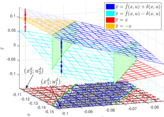
Refer to caption
Figure 2: Illumination of estimating robust NDD 𝕎^𝔉(L)subscript^𝕎𝔉𝐿\hat{\mathbb{W}}_{\mathfrak{F}}(L)

The idea of estimating the RNDD-SC 𝕎𝔉(L)subscript𝕎𝔉𝐿\mathbb{W}_{\mathfrak{F}}(L) is simple. First, generate the sample data set Wdsuperscript𝑊𝑑W^{d} of the interested region 𝕎n+m𝕎superscript𝑛𝑚\mathbb{W}\subset\mathbb{R}^{n+m} under the uniform distribution. Then, find the sample data set W𝔉d(L)Wdsubscriptsuperscript𝑊𝑑𝔉𝐿superscript𝑊𝑑W^{d}_{\mathfrak{F}}(L)\subset W^{d} of 𝕎𝔉(L)subscript𝕎𝔉𝐿\mathbb{W}_{\mathfrak{F}}(L). Finally, The 𝕎𝕎\mathbb{W} is partitioned into disjoint cells and the estimate 𝕎^𝔉(L)subscript^𝕎𝔉𝐿\hat{\mathbb{W}}_{\mathfrak{F}}(L) of 𝕎𝔉(L)subscript𝕎𝔉𝐿\mathbb{W}_{\mathfrak{F}}(L) consists of cells in which all data points belong to W𝔉d(L)subscriptsuperscript𝑊𝑑𝔉𝐿W^{d}_{\mathfrak{F}}(L).

First, let hyper-rectangle 𝕎n+m𝕎superscript𝑛𝑚\mathbb{W}\subset\mathbb{R}^{n+m} denote the interested region. A sample data set Wdsuperscript𝑊𝑑W^{d} of 𝕎𝕎\mathbb{W} can be generated, in which each data point (xd;ud)n+msuperscript𝑥𝑑superscript𝑢𝑑superscript𝑛𝑚(x^{d};u^{d})\in\mathbb{R}^{n+m} is drawn from the uniform distribution on 𝕎𝕎\mathbb{W} and the number of data points is Nxusubscript𝑁xuN_{\text{xu}}. An example of Wdsuperscript𝑊𝑑W^{d} is shown in Figure 2 denoted by blue and red dots in (x(x-u)u)-plane (f^,δ^𝑓𝛿\hat{f},\delta and L𝐿L are the same as those in Example 2).

Then, we aim to find the sample data set W𝔉d(L)Wdsubscriptsuperscript𝑊𝑑𝔉𝐿superscript𝑊𝑑W^{d}_{\mathfrak{F}}(L)\subset W^{d} of 𝕎𝔉(L)subscript𝕎𝔉𝐿\mathbb{W}_{\mathfrak{F}}(L). From (6), any (x;u)𝕎𝔉(L)𝑥𝑢subscript𝕎𝔉𝐿(x;u)\in\mathbb{W}_{\mathfrak{F}}(L) satisfies, x¯𝕏¯𝔉(x,u)for-all¯𝑥subscript¯𝕏𝔉𝑥𝑢\forall\bar{x}\in\bar{\mathbb{X}}_{\mathfrak{F}}(x,u), L(x¯)L(x)<0𝐿¯𝑥𝐿𝑥0L(\bar{x})-L(x)<0. Based on this, the idea of verifying whether a data point (xd;ud)Wdsuperscript𝑥𝑑superscript𝑢𝑑superscript𝑊𝑑(x^{d};u^{d})\in W^{d} belongs to 𝕎𝔉(L)subscript𝕎𝔉𝐿\mathbb{W}_{\mathfrak{F}}(L) is as following. Firstly, for each (xd;ud)Wdsuperscript𝑥𝑑superscript𝑢𝑑superscript𝑊𝑑(x^{d};u^{d})\in W^{d}, a sample data set X¯𝔉d(xd,ud)superscriptsubscript¯𝑋𝔉𝑑superscript𝑥𝑑superscript𝑢𝑑\bar{X}_{\mathfrak{F}}^{d}(x^{d},u^{d}) of 𝕏¯𝔉(xd,ud)subscript¯𝕏𝔉superscript𝑥𝑑superscript𝑢𝑑\bar{\mathbb{X}}_{\mathfrak{F}}(x^{d},u^{d}) is generated, in which each data point x¯dnsuperscript¯𝑥𝑑superscript𝑛\bar{x}^{d}\in\mathbb{R}^{n} is drawn from the uniform distribution on 𝕏¯𝔉(xd,ud)subscript¯𝕏𝔉superscript𝑥𝑑superscript𝑢𝑑\bar{\mathbb{X}}_{\mathfrak{F}}(x^{d},u^{d}) and the number of data points is Nx¯subscript𝑁¯xN_{\mathrm{\bar{x}}}. Secondly, for each (xd;ud)Wdsuperscript𝑥𝑑superscript𝑢𝑑superscript𝑊𝑑(x^{d};u^{d})\in W^{d}, if L(x¯d)L(xd)<0,x¯dX¯𝔉d(xd,ud)formulae-sequence𝐿superscript¯𝑥𝑑𝐿superscript𝑥𝑑0for-allsuperscript¯𝑥𝑑superscriptsubscript¯𝑋𝔉𝑑superscript𝑥𝑑superscript𝑢𝑑L(\bar{x}^{d})-L(x^{d})<0,\forall\bar{x}^{d}\in\bar{X}_{\mathfrak{F}}^{d}(x^{d},u^{d}), (xd;ud)superscript𝑥𝑑superscript𝑢𝑑(x^{d};u^{d}) is deemed to belong to 𝕎𝔉(L)subscript𝕎𝔉𝐿\mathbb{W}_{\mathfrak{F}}(L). Hence, the sample data set

W𝔉d(L)={(xd;ud)Wd|x¯dX¯𝔉d(xd,ud),\displaystyle\!\!W^{d}_{\mathfrak{F}}(L)=\Big{\{}(x^{d};u^{d})\in W^{d}\Big{|}\forall\bar{x}^{d}\in\bar{X}_{\mathfrak{F}}^{d}(x^{d},u^{d}),
L(x¯d)L(xd)<0}\displaystyle\qquad L(\bar{x}^{d})-L(x^{d})<0\Big{\}} (12)

of 𝕎𝔉(L)subscript𝕎𝔉𝐿\mathbb{W}_{\mathfrak{F}}(L) can be obtained. The example of W𝔉d(L)subscriptsuperscript𝑊𝑑𝔉𝐿W^{d}_{\mathfrak{F}}(L) is shown in Figure 2 denoted by blue dots in (x(x-u)u)-plane. For data point (x1d;u1d)2subscriptsuperscript𝑥𝑑1subscriptsuperscript𝑢𝑑1superscript2(x^{d}_{1};u^{d}_{1})\in\mathbb{R}^{2}, 𝕏¯𝔉(x1d,u1d)subscript¯𝕏𝔉subscriptsuperscript𝑥𝑑1subscriptsuperscript𝑢𝑑1\bar{\mathbb{X}}_{\mathfrak{F}}(x^{d}_{1},u^{d}_{1}) is denoted by the blue line segment perpendicular to (x(x-u)u)-plane and sample data set X¯𝔉d(x1d,u1d)superscriptsubscript¯𝑋𝔉𝑑subscriptsuperscript𝑥𝑑1subscriptsuperscript𝑢𝑑1\bar{X}_{\mathfrak{F}}^{d}(x^{d}_{1},u^{d}_{1}) is denoted by blue ’x’. For (x2d;u2d)2subscriptsuperscript𝑥𝑑2subscriptsuperscript𝑢𝑑2superscript2(x^{d}_{2};u^{d}_{2})\in\mathbb{R}^{2}, 𝕏¯𝔉(x2d,u2d)subscript¯𝕏𝔉subscriptsuperscript𝑥𝑑2subscriptsuperscript𝑢𝑑2\bar{\mathbb{X}}_{\mathfrak{F}}(x^{d}_{2},u^{d}_{2}) is denoted by the red line segment and sample data set X¯𝔉d(x2d,u2d)superscriptsubscript¯𝑋𝔉𝑑subscriptsuperscript𝑥𝑑2subscriptsuperscript𝑢𝑑2\bar{X}_{\mathfrak{F}}^{d}(x^{d}_{2},u^{d}_{2}) is denoted by red ’x’. Because all x¯dX¯𝔉d(x1d,u1d)superscript¯𝑥𝑑superscriptsubscript¯𝑋𝔉𝑑subscriptsuperscript𝑥𝑑1subscriptsuperscript𝑢𝑑1\bar{x}^{d}\in\bar{X}_{\mathfrak{F}}^{d}(x^{d}_{1},u^{d}_{1}) are between the surfaces x¯=x¯𝑥𝑥\bar{x}=x and x¯=x¯𝑥𝑥\bar{x}=-x, namely L(x¯d)L(xd)<0𝐿superscript¯𝑥𝑑𝐿superscript𝑥𝑑0L(\bar{x}^{d})-L(x^{d})<0, (x1d;u1d)subscriptsuperscript𝑥𝑑1subscriptsuperscript𝑢𝑑1(x^{d}_{1};u^{d}_{1}) is collected by data set W𝔉d(L)subscriptsuperscript𝑊𝑑𝔉𝐿W^{d}_{\mathfrak{F}}(L), while (x2d;u2d)subscriptsuperscript𝑥𝑑2subscriptsuperscript𝑢𝑑2(x^{d}_{2};u^{d}_{2}) is not.

Finally, the interested region 𝕎𝕎\mathbb{W} is partitioned into disjoint cells. Here, we apply a uniform grid over 𝕎𝕎\mathbb{W} and each cell is a rectangle or hyper-rectangle. Suppose there are Ncsubscript𝑁cN_{\text{c}} cells in the grid and each cell is denoted by i,i=1,2,,Ncformulae-sequencesubscript𝑖𝑖12subscript𝑁c\mathbb{C}_{i},i=1,2,\cdots,N_{\text{c}}. An inner approximation 𝕎^𝔉(L)subscript^𝕎𝔉𝐿\hat{\mathbb{W}}_{\mathfrak{F}}(L) of 𝕎𝔉(L)subscript𝕎𝔉𝐿\mathbb{W}_{\mathfrak{F}}(L) can be obtained by combining all cells only containing data points in W𝔉d(L)subscriptsuperscript𝑊𝑑𝔉𝐿W^{d}_{\mathfrak{F}}(L). The example of 𝕎^𝔉(L)subscript^𝕎𝔉𝐿\hat{\mathbb{W}}_{\mathfrak{F}}(L) is shown in Figure 2 denoted by gray rectangles in (x(x-u)u)-plane. Figure 2 also shows 𝕎𝔉(L)subscript𝕎𝔉𝐿\mathbb{W}_{\mathfrak{F}}(L) denoted by the domain between the two green curves in (x(x-u)u)-plane and Π𝔉(L)subscriptΠ𝔉𝐿\Pi_{\mathfrak{F}}(L) denoted by the 3-dimensional domain between the blue surface, the cyan surface and the two green surfaces.

The above procedure is summarized in Algorithm 1.

Algorithm 1 Robust NDDs estimation algorithm

For the given positive-definite function L𝐿L, plant set 𝔉𝔉\mathfrak{F} and grid over 𝕎𝕎\mathbb{W}, estimates 𝕎^𝔉(L)subscript^𝕎𝔉𝐿\hat{\mathbb{W}}_{\mathfrak{F}}(L) and 𝕏^𝔉(L)subscript^𝕏𝔉𝐿\hat{\mathbb{X}}_{\mathfrak{F}}(L) of RNDDs can be obtained as the following:

1:Generate the sample data set Wdsuperscript𝑊𝑑W^{d} whose data points are drawn from the uniform distribution on 𝕎𝕎\mathbb{W};
2:For each data point (xd;ud)Wdsuperscript𝑥𝑑superscript𝑢𝑑superscript𝑊𝑑(x^{d};u^{d})\in W^{d}, generate the sample data set X¯𝔉d(xd,ud)subscriptsuperscript¯𝑋𝑑𝔉superscript𝑥𝑑superscript𝑢𝑑\bar{X}^{d}_{\mathfrak{F}}(x^{d},u^{d}) whose data points are drawn from the uniform distribution on 𝕏¯𝔉(xd,ud)subscript¯𝕏𝔉superscript𝑥𝑑superscript𝑢𝑑\bar{\mathbb{X}}_{\mathfrak{F}}(x^{d},u^{d});
3:Find the sample data set W𝔉d(L)subscriptsuperscript𝑊𝑑𝔉𝐿W^{d}_{\mathfrak{F}}(L) defined in (12) by selecting data point (xd;ud)Wdsuperscript𝑥𝑑superscript𝑢𝑑superscript𝑊𝑑(x^{d};u^{d})\in W^{d} which satisfies L(x¯d)L(xd)<0,x¯dX¯𝔉d(xd,ud)formulae-sequence𝐿superscript¯𝑥𝑑𝐿superscript𝑥𝑑0for-allsuperscript¯𝑥𝑑superscriptsubscript¯𝑋𝔉𝑑superscript𝑥𝑑superscript𝑢𝑑L(\bar{x}^{d})-L(x^{d})<0,\forall\bar{x}^{d}\in\bar{X}_{\mathfrak{F}}^{d}(x^{d},u^{d});
4:Obtain the estimate 𝕎^𝔉(L)subscript^𝕎𝔉𝐿\hat{\mathbb{W}}_{\mathfrak{F}}(L) of 𝕎𝔉(L)𝕎subscript𝕎𝔉𝐿𝕎\mathbb{W}_{\mathfrak{F}}(L)\subset\mathbb{W} by combining all cells only containing data points in W𝔉d(L)subscriptsuperscript𝑊𝑑𝔉𝐿W^{d}_{\mathfrak{F}}(L);
5:Obtain the estimate 𝕏^𝔉(L)subscript^𝕏𝔉𝐿\hat{\mathbb{X}}_{\mathfrak{F}}(L) of 𝕏𝔉(L)subscript𝕏𝔉𝐿\mathbb{X}_{\mathfrak{F}}(L) by projecting 𝕎^𝔉(L)subscript^𝕎𝔉𝐿\hat{\mathbb{W}}_{\mathfrak{F}}(L) along the control space onto the state space.
Remark 5.

In Step 1 and 2, Algorithm 1 generates Nxu(n+m)+NxuNx¯nsubscript𝑁𝑥𝑢𝑛𝑚subscript𝑁𝑥𝑢subscript𝑁¯𝑥𝑛N_{xu}(n+m)+N_{xu}N_{\bar{x}}n random numbers. In Step 3, the number of verification of L(x¯)dL(xd)<0𝐿superscript¯𝑥𝑑𝐿superscript𝑥𝑑0L(\bar{x})^{d}-L(x^{d})<0 is NxuNx¯subscript𝑁𝑥𝑢subscript𝑁¯𝑥N_{xu}N_{\bar{x}}. In Step 4, the number of verification whether or not a cell satisfies that all data points in it belong to W𝔉d(L)subscriptsuperscript𝑊𝑑𝔉𝐿W^{d}_{\mathfrak{F}}(L) is Ncsubscript𝑁𝑐N_{c}. It is hard to find a quantitative analysis result about the precision of Algorithm 1 because it uses the random sampling and griding method to approximate the desired domain. We can only declare that, in order to obtain a good estimation, Nxu,Nx¯subscript𝑁𝑥𝑢subscript𝑁¯𝑥N_{xu},N_{\bar{x}} and Ncsubscript𝑁𝑐N_{c} must be enough large.

4.2 Estimating robust DOA of closed-loops and designing controller

The RNDD-SC 𝕎𝔉(L)subscript𝕎𝔉𝐿\mathbb{W}_{\mathfrak{F}}(L) defined in (6) is an open set and the origin (0;0)n+m00superscript𝑛𝑚(0;0)\in\mathbb{R}^{n+m} is in the boundary of 𝕎𝔉(L)subscript𝕎𝔉𝐿\mathbb{W}_{\mathfrak{F}}(L). There is no cell belonging to the inner approximation 𝕎^𝔉(L)subscript^𝕎𝔉𝐿\hat{\mathbb{W}}_{\mathfrak{F}}(L) nearby the origin (0;0)n+m00superscript𝑛𝑚(0;0)\in\mathbb{R}^{n+m} and there is a small neighborhood 𝕏0nsubscript𝕏0superscript𝑛\mathbb{X}_{0}\subset\mathbb{R}^{n} of the origin in the state space that is not contained by the projection 𝕏^𝔉(L)subscript^𝕏𝔉𝐿\hat{\mathbb{X}}_{\mathfrak{F}}(L) of 𝕎^𝔉(L)subscript^𝕎𝔉𝐿\hat{\mathbb{W}}_{\mathfrak{F}}(L). Hence, the condition (9) of estimating RDOA in Theorem 3 is modified as 𝕏ls(L,α)𝕏^𝔉(L)𝕏0subscript𝕏ls𝐿𝛼subscript^𝕏𝔉𝐿subscript𝕏0\mathbb{X}_{\text{ls}}(L,\alpha)\subset\hat{\mathbb{X}}_{\mathfrak{F}}(L)\cup\mathbb{X}_{0}. Note that the volume of 𝕏ls(L,α)subscript𝕏ls𝐿𝛼\mathbb{X}_{\text{ls}}(L,\alpha) is increasing as α𝛼\alpha is increasing for a given Lyapunov function L𝐿L. Hence, the largest estimate of RDOA can be obtained by solving the optimization problem

maxα+αsubject to 𝕏ls(L,α)𝕏^𝔉(L)𝕏0.subscript𝛼subscript𝛼subject to subscript𝕏ls𝐿𝛼subscript^𝕏𝔉𝐿subscript𝕏0\displaystyle\max_{\alpha\in\mathbb{R}_{+}}\alpha\quad\text{subject to }\mathbb{X}_{\text{ls}}(L,\alpha)\subset\hat{\mathbb{X}}_{\mathfrak{F}}(L)\cup\mathbb{X}_{0}. (13)

In order to verify the constrains in (13), it is needed to estimate the level-set 𝕏ls(L,α)subscript𝕏ls𝐿𝛼\mathbb{X}_{\text{ls}}(L,\alpha). With the same idea of estimating the RNDD-SC 𝕎𝔉(L)subscript𝕎𝔉𝐿\mathbb{W}_{\mathfrak{F}}(L), the estimate of 𝕏ls(L,α)subscript𝕏ls𝐿𝛼\mathbb{X}_{\text{ls}}(L,\alpha) can be obtained. Let αsuperscript𝛼\alpha^{\ast} be the solution of (13). The estimate of RDOA is 𝕏ls(L,α)subscript𝕏ls𝐿superscript𝛼\mathbb{X}_{\text{ls}}(L,\alpha^{\ast}).

Replacing the RNDD-SC 𝕎𝔉(L)n+msubscript𝕎𝔉𝐿superscript𝑛𝑚\mathbb{W}_{\mathfrak{F}}(L)\subset\mathbb{R}^{n+m} with its estimate 𝕎^𝔉(L)subscript^𝕎𝔉𝐿\hat{\mathbb{W}}_{\mathfrak{F}}(L), from Theorem 3, we know that any controller μ𝜇\mu belonging to 𝕎^𝔉(L)subscript^𝕎𝔉𝐿\hat{\mathbb{W}}_{\mathfrak{F}}(L) can stabilize all plants in 𝔉𝔉\mathfrak{F}. A simple way to find a controller μ𝜇\mu belonging to 𝕎^𝔉(L)subscript^𝕎𝔉𝐿\hat{\mathbb{W}}_{\mathfrak{F}}(L) is that, first, select a controller training set belonging to 𝕎^𝔉(L)subscript^𝕎𝔉𝐿\hat{\mathbb{W}}_{\mathfrak{F}}(L); then, obtain the controller μ𝜇\mu with a function estimation method, such as interpolation, Gaussian processes regression and so on. When the trend of the training data points is smooth enough and μ(0)=0𝜇00\mu(0)=0 is constrained, it can be guaranteed that the controller obtained from the function estimator belongs to 𝕎^𝔉(L)subscript^𝕎𝔉𝐿\hat{\mathbb{W}}_{\mathfrak{F}}(L).

Refer to caption
Refer to caption

(a)

(b)

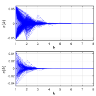
Figure 3: (a) Estimates 𝕎^𝔉(L)subscript^𝕎𝔉𝐿\hat{\mathbb{W}}_{\mathfrak{F}}(L), 𝕏^𝔉(L)subscript^𝕏𝔉𝐿\hat{\mathbb{X}}_{\mathfrak{F}}(L) of robust NDDs, estimate 𝕏ls(L,0.0036)subscript𝕏ls𝐿0.0036\mathbb{X}_{\text{ls}}(L,0.0036) of robust DOA for closed-loops, controller training data and robust controller μ𝜇\mu. (b) State trajectories of closed-loops and noise trajectories.

The method proposed in this section is verified in the following example.

Example 6.

Consider f^,δ^𝑓𝛿\hat{f},\delta and L𝐿L in Example 2. The interested region 𝕎=[0.3,0.3]×[0.3,0.3]2𝕎0.30.30.30.3superscript2\mathbb{W}=[-0.3,0.3]\times[-0.3,0.3]\subset\mathbb{R}^{2} in the state-control space is partitioned into 9×1049superscript1049\times 10^{4} cells of size 0.002×0.0020.0020.0020.002\times 0.002. The number of data points in Wdsuperscript𝑊𝑑W^{d} is selected as 106superscript10610^{6}. For each data point (xd;ud)superscript𝑥𝑑superscript𝑢𝑑(x^{d};u^{d}) in Wdsuperscript𝑊𝑑W^{d}, the number of data points in X¯𝔉d(xd,ud)subscriptsuperscript¯𝑋𝑑𝔉superscript𝑥𝑑superscript𝑢𝑑\bar{X}^{d}_{\mathfrak{F}}(x^{d},u^{d}) is selected as 200200200. Using Algorithm 1, an estimate 𝕎^𝔉(L)subscript^𝕎𝔉𝐿\hat{\mathbb{W}}_{\mathfrak{F}}(L) of the RNDD-SC 𝕎𝔉(L)subscript𝕎𝔉𝐿\mathbb{W}_{\mathfrak{F}}(L) is obtained and shown in Figure 3 (a) denoted by gray region. An estimate 𝕏^𝔉(L)subscript^𝕏𝔉𝐿\hat{\mathbb{X}}_{\mathfrak{F}}(L) of the RNDD-S 𝕏𝔉(L)subscript𝕏𝔉𝐿\mathbb{X}_{\mathfrak{F}}(L) is also obtained and shown in Figure 3 (a) denoted by green line segment in x𝑥x-axis, where the neighborhood 𝕏0subscript𝕏0\mathbb{X}_{0} of the origin that is not contained by 𝕏^𝔉(L)subscript^𝕏𝔉𝐿\hat{\mathbb{X}}_{\mathfrak{F}}(L) is [0.004,0.004]0.0040.004[-0.004,0.004].

By solving the optimization problem (13), we obtain the largest level-set 𝕏ls(L,0.0036)=[0.06,0.06]subscript𝕏ls𝐿0.00360.060.06\mathbb{X}_{\text{ls}}(L,0.0036)=[-0.06,0.06]\subset\mathbb{R} of L(x)=x2𝐿𝑥superscript𝑥2L(x)=x^{2} as the estimate of the RDOA for closed-loops, which is shown in Figure 3 (a) denoted by the blue line segment in x𝑥x-axis. In order to find a controller μ𝜇\mu belonging to the gray region, we select a training data set shown by red ’x’ in Figure 3 (a). A robust controller μ𝜇\mu is obtained using Gaussian processes regression, as shown in Figure 3 (a) denoted by black line.

To verify whether the controller μ𝜇\mu can stabilize all plants in the plant set for all initial state in 𝕏ls(L,0.0036)subscript𝕏ls𝐿0.0036\mathbb{X}_{\text{ls}}(L,0.0036), we consider the controlled system x(k+1)=f^(x(k),u(k))+e(k)𝑥𝑘1^𝑓𝑥𝑘𝑢𝑘𝑒𝑘x(k+1)=\hat{f}(x(k),u(k))+e(k), where noise e(k)𝑒𝑘e(k) is drawn from the uniform distribution on [δ(k),δ(k)]𝛿𝑘𝛿𝑘[-\delta(k),\delta(k)]\subset\mathbb{R} and δ(k)=δ(x(k),u(k))𝛿𝑘𝛿𝑥𝑘𝑢𝑘\delta(k)=\delta(x(k),u(k)). Figure 3 (b) shows 1000 state trajectories of x(k+1)=f^(x(k),μ(x(k)))+e(k)𝑥𝑘1^𝑓𝑥𝑘𝜇𝑥𝑘𝑒𝑘x(k+1)=\hat{f}(x(k),\mu(x(k)))+e(k), whose initial states are drawn from the uniform distribution on 𝕏ls(L,0.0036)subscript𝕏ls𝐿0.0036\mathbb{X}_{\text{ls}}(L,0.0036). We see that all state trajectories converge to the origin. Figure 3 (b) also shows 1000 noises trajectories corresponding to the 1000 state trajectories.

5 Conclusion

In order to overcome the drawback of existing nonlinear robust control approaches, this paper proposes a new robust control method where the uncertain system is described by a non-affine nonlinear plant set. Under this circumstance, it is in general hard to fulfill the global stabilization, which requests an extensive investigation about the robust DOA of closed-loops. To this end, the sufficient condition is presented for robust asymptotic stabilization of the plant set and estimation of the RDOA for closed-loops. Moreover, due to non-affine nonlinearities, it is hard to obtain analytic solutions of the RNDDs. To overcome this problem, a data-driven method of estimating the RNDDs is proposed.

References

  • [1] T. Basar and J. W. Helton. H-infinity-Optimal Control and Related Minimax Design Problems. Birkhauser, Boston, second edition, 1995.
  • [2] S. P. Bhattacharyya. Robust control under parametric uncertainty: An overview and recent results. Annual Reviews in Control, 44:45–77, 2017.
  • [3] Y. Chen, M. Tanaka, K. Tanaka, and H. O. Wang. Stability analysis and region-of- attraction estimation using piecewise polynomial lyapunov functions: Polynomial fuzzy model approach. Ieee Transactions on Fuzzy Systems, 23(4):1314–1322, 2015.
  • [4] M. J. Corless. Robust stability analysis and controller design with quadratic Lyapunov functions. Springer-Verlag, Berlin, 1993.
  • [5] R. A. Freeman and P. Kokotovic. Robust Nonlinear Control Design: State-Space and Lyapunov Techniques. Birkhauser, Boston, 2008.
  • [6] S. Gering, L. Eciolaza, J. Adamy, and M. Sugeno. A piecewise approximation approach to nonlinear systems: Stability and region of attraction. Ieee Transactions on Fuzzy Systems, 23(6):2231–2244, 2015.
  • [7] A. Goldsztejn and G. Chabert. Estimating the robust domain of attraction for non-smooth systems using an interval lyapunov equation. Automatica, 100:371–377, 2019.
  • [8] W. M. Haddad and V. Chellaboina. Nonlinear Dynamical Systems and Control: A Lyapunov-Based Approach. Princeton University Press, New Jersey, 2008.
  • [9] Y. Li and Z. Hou. Data-driven asymptotic stabilization for discrete-time nonlinear systems. Systems & Control Letters, 64:79–85, 2014.
  • [10] I. R. Petersen and R. Tempo. Robust control of uncertain systems: Classical results and recent developments. Automatica, 50(5):1315–1335, 2014.
  • [11] C. E. Rasmussen and C. K. I. Williams. Gaussian Processes for Machine Learning. MIT Press, 2006.
  • [12] M. G. Safonov. Origins of robust control: Early history and future speculations. Annual Reviews in Control, 36(2):173–181, 2012.
  • [13] E. D. Sontag and Y. Wang. On characterizations of the input-to-state stability property. Systems & Control Letters, 24:351–359, 1995.
  • [14] S. H. Tsai and C. Y. Jen. H-infinity stabilization for polynomial fuzzy time-delay system: A sum-of-squares approach. IEEE Transactions on Fuzzy Systems, 26(6):3630–3644, 2018.