Entropy Stable $p$-Nonconforming Discretizations with the Summation-by-Parts Property for the Compressible Navier–Stokes Equations

Abstract

The entropy conservative, curvilinear, nonconforming, $p$-refinement algorithm for hyperbolic conservation laws of Del Rey Fernández et al. (2019), is extended from the compressible Euler equations to the compressible Navier–Stokes equations. A simple and flexible coupling procedure with planar interpolation operators between adjoining nonconforming elements is used. Curvilinear volume metric terms are numerically approximated via a minimization procedure and satisfy the discrete geometric conservation law conditions. Distinct curvilinear surface metrics are used on the adjoining interfaces to construct the interface coupling terms, thereby localizing the discrete geometric conservation law constraints to each individual element. The resulting scheme is entropy conservative/stable, element-wise conservative, and freestream preserving. Viscous interface dissipation operators are developed that retain the entropy stability of the base scheme. The accuracy and stability properties of the resulting numerical scheme are shown to be comparable to those of the original conforming scheme (achieving $\sim p+1$ convergence) in the context of the viscous shock problem, the Taylor–Green vortex problem at a Reynolds number of $Re=1,600$, and a subsonic turbulent flow past a sphere at $Re=2,000$.

1 Introduction

For a certain class of partial differential equations (PDEs), such as the linear wave propagation, high-order accurate methods are known to be more efficient than low order methods [1, 2]. Moreover, high-order methods are well suited to exploit the exascale concurrency on next generation hardware because their computational kernels are arithmetically dense and typically local (see, for instance, [3, 4]). Nevertheless, despite their long history of development, their application to nonlinear PDEs for practical application has been limited by robustness issues, particularly in the context of $h$-, $p$-, and $r$-refinement algorithms to better resolve multi-scale physics. Thus, nominally second-order accurate discretization operators have dominated commercial software development.

In the context of linear and variable coefficient problems, the summation-by-parts (SBP) framework provides a systematic and discretization-agnostic methodology for the design and analysis of arbitrarily high order, provably conservative and stable numerical methods (see the review papers [5, 6]). SBP operators are matrix difference operators that come endowed with a high-order accurate approximation to integration by parts (IBP) that telescopes (i.e., results in boundary terms). Over each element, the mimetic and telescoping properties allow a one-to-one match between discrete and continuous stability proofs. The stability of the full spatial discretization is achieved by combining the local SBP mechanics with suitable inter-element coupling and boundary conditions procedures (e.g., the simultaneous approximation terms (SATs) [7, 8, 9, 10, 11, 12, 13, 14, 15]).

For nonlinear problems, a provable stability analysis and general theory at the discrete level has remained far more elusive. Nonetheless, progress has been made, in particular, Tadmor [16] developed entropy conservative/stable low order finite volume schemes that achieve entropy conservation by using two-point flux functions that when contracted with the entropy variables result in a telescoping entropy flux. Entropy stability results by adding appropriate dissipation. Via the telescoping property, the continuous $L^{2}$ entropy stability analysis is mimicked by the semi-discrete stability analysis (for a complete exposition of these ideas, see Tadmor [17]). The essence of Tadmor’s approach resulted in the construction of numerous entropy stable schemes. For example, Fjordholm et al. [18] have constructed high-order accurate essentially non-oscillatory schemes and Ray et al. [19] have constructed low-order accurate unstructured finite volume discretizations.

Fisher and co-authors extended Tadmor’s approach to finite domains by combining the SBP framework with Tadmor’s two point flux functions [20, 21, 22] to construct entropy stable semi-discrete schemes (see also the related work [23, 24]). Since then, these ideas have been extended in numerous ways (e.g. Refs. [25, 26, 27, 28, 29, 30, 31, 32, 33, 34, 35, 36, 37]). This combination is attractive because it inherits all of the mechanics of SBP schemes for the imposition of boundary conditions and inter-element coupling and therefore gives a systematic methodology for discretizing problems on complex geometries [25, 14]. Furthermore, the resulting discrete stability proofs do not rely on the assumption of exact integration (see for example the work of Hughes et al. [38]). Recently, these ideas have been extended to achieve fully-discrete explicit entropy stable schemes for the compressible Euler [39] and Navier–Stokes equations [40].

An alternative approach, developed by Olsson and Oliger [41], Gerritsen and Olsson [42] and Yee et al. [43] (see also [44, 24]), is based upon choosing entropy functions that result in a homogeneity property on the compressible Euler fluxes. Using this property, the Euler fluxes can be split such that when contracted with the entropy variables stability estimates result that are analogous in form to energy estimates obtained for linear PDEs.

The objective herein, is to construct entropy stable discretizations for the compressible Navier–Stokes equations (NSE), applicable to high-order accurate $p$-adaptivity. The work is a natural extension of the entropy stable $p$-refinement algorithm for the compressible Euler equations in Refs. [45, 46]. The inviscid terms in the NSE are discretized without modifications using an existing approach [25, 47, 14, 27]. The inviscid discretization requires two sets of metrics: 1) volume metrics determined numerically by solving a discrete Geometric Conservation Law (GCL) constraint, and 2) surface metric terms that are specified. Viscous terms are discretized using a local discontinuous Galerkin (LDG) approach, plus interior penalty (IP) dissipation included on interfaces. The discretization of the viscous terms is a natural extension of the curvilinear LDG-IP approaches found in [25, 47, 14, 27], to include non-conforming interfaces, and are entropy stable by construction.

The contributions of the paper are summarized as follows:

• The LDG-IP approach in Refs. [25, 47, 14, 27] is applied and extended to the curvilinear nonconforming interface problem.

  • The viscous operator, written in terms of the entropy variables, is discretized using an LDG approach with macro-element discretizations. A provably stable quadratic form results, provided that identical metrics are used in (both) curvilinear transformations.

  • Viscous interface dissipation (the IP terms) are a generalization of the inviscid nonconforming interface dissipation. A novel average of on-element and interpolated off-element data leads immediately to an entropy stable IP term.

  • The resulting scheme is entropy stable and freestream preserving.

• Numerical evidence is provided demonstrating that the nonconforming algorithm 1) retains similar non-linear robustness properties and 2) achieves similar $L^{2}$-norm convergence rates, i.e., $\sim p+1$ (where $p$ is the highest degree polynomial exactly differentiated by the differentiation operator) as that of the original nonlinearly stable conforming algorithm [25, 27]

The paper is organized as follows. Section 2 delineates the notation used herein. Section 3 reviews the nonconforming algorithm for hyperbolic conservation laws of Del Rey Fernández et al. [45, 48] in the context of the linear convection equation. The extension to viscous terms is demonstrated by considering the convection-diffusion equation. The application of the nonconforming algorithm to the viscous components of the compressible Navier–Stokes equations is detailed in Section 4 while numerical experiments are presented in Section 5. Finally, conclusions are drawn in Section 6.

2 Notation

The notation used herein is identical to that in [45]; readers familiar with the notation can skip to Section 3. PDEs are discretized on cubes having Cartesian computational coordinates denoted by the triple $(\xi_{1},\xi_{2},\xi_{3})$, where the physical coordinates are denoted by the triple $(x_{1},x_{2},x_{3})$. Vectors are represented by lowercase bold font, for example $\bm{u}$, while matrices are represented using sans-serif font, for example, $\mathsf{B}$. Continuous functions on a space-time domain are denoted by capital letters in script font. For example,

$$\mathcal{U}\left(\xi_{1},\xi_{2},\xi_{3},t\right)\in L^{2}\left(\left[\alpha_{1},\beta_{1}\right]\times\left[\alpha_{2},\beta_{2}\right]\times\left[\alpha_{3},\beta_{3}\right]\times\left[0,T\right]\right)$$

represents a square integrable function, where $t$ is the temporal coordinate. The restriction of such functions onto a set of mesh nodes is denoted by lower case bold font. For example, the restriction of $\mathcal{U}$ onto a grid of $N_{1}\times N_{2}\times N_{3}$ nodes is given by the vector

$$\bm{u}=\left[\mathcal{U}\left(\bm{\xi}^{(1)},t\right),\dots,\mathcal{U}\left(\bm{\xi}^{(N)},t\right)\right]^{\mathrm{T}},$$

where, $N$ is the total number of nodes ($N\equiv N_{1}N_{2}N_{3}$) square brackets ($[]$) are used to delineate vectors and matrices as well as ranges for variables (the context will make clear which meaning is being used). Moreover, $\bm{\xi}$ is a vector of vectors constructed from the three vectors $\bm{\xi}_{1}$, $\bm{\xi}_{2}$, and $\bm{\xi}_{3}$, which are vectors of size $N_{1}$, $N_{2}$, and $N_{3}$ and contain the coordinates of the mesh in the three computational directions, respectively. Finally, $\bm{\xi}$ is constructed as

$$\bm{\xi}(3(i-1)+1:3i)\equiv\bm{\xi}^{(i)}\equiv\left[\bm{\xi}_{1}(i),\bm{\xi}_{2}(i),\bm{\xi}_{3}(i)\right]^{\mathrm{T}},$$

where the notation $\bm{u}(i)$ means the $i^{\mathrm{th}}$ entry of the vector $\bm{u}$ and $\bm{u}(i:j)$ is the subvector constructed from $\bm{u}$ using the $i^{\mathrm{th}}$ through $j^{\mathrm{th}}$ entries (i.e., Matlab notation is used).

Oftentimes, monomials are discussed and the following notation is used:

$$\bm{\xi}_{l}^{j}\equiv\left[\left(\bm{\xi}_{l}(1)\right)^{j},\dots,\left(\bm{\xi}_{l}(N_{l})\right)^{j}\right]^{\mathrm{T}},$$

and the convention that $\bm{\xi}_{l}^{j}=\bm{0}$ for $j<0$ is used.

Herein, one-dimensional SBP operators are used to discretize derivatives. The definition of a one-dimensional SBP operator in the $\xi_{l}$ direction, $l=1,2,3$, is [49, 5, 6]

Definition 1.

Summation-by-parts operator for the first derivative: A matrix operator, $\mathsf{D}_{\xi_{l}}^{(1D)}\in\mathbb{R}^{N_{l}\times N_{l}}$, is an SBP operator of degree $p$ approximating the derivative $\frac{\partial}{\partial\xi_{l}}$ on the domain $\xi_{l}\in\left[\alpha_{l},\beta_{l}\right]$ with nodal distribution $\bm{\xi}_{l}$ having $N_{l}$ nodes, if

1. $\mathsf{D}_{\xi_{l}}^{(1D)}\bm{\xi}_{l}^{j}=j\bm{\xi}_{l}^{j-1}$, $j=0,1,\dots,p$;

2. $\mathsf{D}_{\xi_{l}}^{(1D)}\equiv\left(\mathsf{P}_{\xi_{l}}^{(1D)}\right)^{-1}\mathsf{Q}_{\xi_{l}}^{(1D)}$, where the norm matrix, $\mathsf{P}_{\xi_{l}}^{(1D)}$, is symmetric positive definite;

3. $\mathsf{Q}_{\xi_{l}}^{(1D)}\equiv\left(\mathsf{S}_{\xi_{l}}^{(1D)}+\frac{1}{2}\mathsf{E}_{\xi_{l}}^{(1D)}\right)$, $\mathsf{S}_{\xi_{l}}^{(1D)}=-\left(\mathsf{S}_{\xi_{l}}^{(1D)}\right)^{\mathrm{T}}$, $\mathsf{E}_{\xi_{l}}^{(1D)}=\left(\mathsf{E}_{\xi_{l}}^{(1D)}\right)^{\mathrm{T}}$, $\mathsf{E}_{\xi_{l}}^{(1D)}=\operatorname{diag}\left(-1,0,\dots,0,1\right)=\bm{e}_{N_{l}}\bm{e}_{N_{l}}^{\mathrm{T}}-\bm{e}_{1_{l}}\bm{e}_{1_{l}}^{\mathrm{T}}$, $\bm{e}_{1_{l}}\equiv\left[1,0,\dots,0\right]^{\mathrm{T}}$, and $\bm{e}_{N_{l}}\equiv\left[0,0,\dots,1\right]^{\mathrm{T}}$.

Thus, a degree $p$ SBP operator is one that differentiates exactly monomials up to degree $p$.

In this work, one-dimensional SBP operators are extended to multiple dimensions using tensor products ($\otimes$). The tensor product between the matrices $\mathsf{A}$ and $\mathsf{B}$ is given as $\mathsf{A}\otimes\mathsf{B}$. When referencing individual entries in a matrix the notation $\mathsf{A}(i,j)$ is used, which means the $i^{\mathrm{th}}$ $j^{\mathrm{th}}$ entry in the matrix $\mathsf{A}$.

The focus in this paper is exclusively on diagonal-norm SBP operators. Moreover, the same one-dimensional SBP operator are used in each direction, each operating on $N$ nodes. Specifically, diagonal-norm SBP operators constructed on the Legendre–Gauss–Lobatto (LGL) nodes are used, i.e., a discontinuous Galerkin collocated spectral element approach is utilized.

The physical domain $\Omega\subset\mathbb{R}^{3}$, with boundary $\Gamma\equiv\partial\Omega$ is partitioned into $K$ non-overlapping hexahedral elements. The domain of the $\kappa^{\text{th}}$ element is denoted by $\Omega_{\kappa}$ and has boundary $\partial\Omega_{\kappa}$. Numerically, PDEs are solved in computational coordinates, where each $\Omega_{\kappa}$ is locally transformed to $\hat{\Omega}_{\kappa}$, with boundary $\hat{\Gamma}\equiv\partial\hat{\Omega}_{\kappa}$, under the following assumption:

Assumption 1.

Each element in physical space is transformed using a local and invertible curvilinear coordinate transformation that is compatible at shared interfaces, meaning that points in computational space on either side of a shared interface mapped to the same physical location and therefore map back to the analogous location in computational space; this is the standard assumption that the curvilinear coordinate transformation is water tight.

3 A $p$-nonconforming algorithm: Linear convection-diffusion equation

The focus in this paper is on curvilinearly mapped elements with conforming interfaces but nonconforming nodal distributions, as occurs, for example, in $p$-refinement. The construction of entropy conservative/stable discretizations for the compressible Euler equations on Cartesian grids is detailed in Friedrich et al. [46]. The extension to curvilinear coordinates is covered in [45, 48] where a $p$-refinement, curvilinear, interface coupling technique that maintains 1) accuracy, 2) discrete entropy conservation/stability, and 3) element-wise conservation is presented. Herein, the technology presented in [45, 48] is extended to the discretization of the viscous portion of the compressible Navier–Stokes equations.

3.1 Scalar convection-diffusion equation: Continuous and semi-discrete analysis

Many of the technical challenges in constructing conservative and stable nonconforming discretizations for the compressible Navier–Stokes equations are also present in the discretization of the linear convection-diffusion equation. For this reason, the interface coupling procedure for the inviscid terms shown in [45, 48] as well as their extension to viscous terms (the focus of this paper) is presented in the context of this simple linear scalar equation. The linear convection-diffusion equation in Cartesian coordinates is given as

$$\frac{\partial\mathcal{U}}{\partial t}+\sum\limits_{m=1}^{3}\frac{\partial\left(a_{m}\mathcal{U}\right)}{\partial x_{m}}=\sum\limits_{m=1}^{3}\frac{\partial^{2}(b_{m}\mathcal{U})}{\partial x_{m}^{2}},$$ (1)

where $(a_{m}\mathcal{U})$ are the inviscid fluxes, $a_{m}$ are the (constant) components of the convection speed, $\frac{\partial(b_{m}\mathcal{U})}{\partial x_{m}}$ are the viscous fluxes, and $b_{m}$ are the (constant and positive) diffusion coefficients. The energy method can be used to determine the stability of (1). It proceeds by multiplying (1) by the solution, ($\mathcal{U}$), and after using the chain rule yields

$$\frac{1}{2}\frac{\partial\mathcal{U}^{2}}{\partial t}+\frac{1}{2}\sum\limits_{m=1}^{3}\frac{\partial\left(a_{m}\mathcal{U}^{2}\right)}{\partial x_{m}}=\sum\limits_{m=1}^{3}\left\{\frac{\partial}{\partial x_{m}}\left(\mathcal{U}\frac{\partial(b_{m}\mathcal{U})}{\partial x_{m}}\right)-\left(\frac{\partial(b_{m}\mathcal{U})}{\partial x_{m}}\right)^{2}\right\}.$$ (2)

Integrating over the domain, $\Omega$, using the integration by parts, and the Leibniz rule yields

$$\begin{split}&\frac{\mathrm{d}}{\mathrm{d}t}\int_{\Omega}\frac{\mathcal{U}^{2}}{2}\mathrm{d}\Omega+\\ &\frac{1}{2}\sum\limits_{m=1}^{3}\left(\oint_{\Gamma}\left\{\left(a_{m}\mathcal{U}^{2}\right)-2\mathcal{U}\frac{(b_{m}\mathcal{U})}{\partial x_{m}}\right\}n_{x_{m}}\mathrm{d}\Gamma+2\int_{\Omega}\left(\frac{\partial(b_{m}\mathcal{U})}{\partial x_{m}}\right)^{2}\mathrm{d}\Omega\right)=0,\end{split}$$ (3)

with $n_{x_{m}}$ the $m^{\mathrm{th}}$ component of the outward facing unit normal. Eq. (3) demonstrates that the time rate of change of the norm of the solution, $\|\mathcal{U}\|^{2}\equiv\int_{\Omega}\mathcal{U}^{2}\mathrm{d}\Gamma$, depends on surface flux integrals and a viscous dissipation term. Therefore, if appropriate boundary conditions are imposed, Eq. (3) leads to an energy estimate on the solution and, hence, a proof of stability. The SBP framework used in this paper mimics the above energy stability analysis in a one-to-one fashion and leads to similar stability statements on the semi-discrete equations.

Derivatives are approximated using differentiation matrices that are defined in computational space and for this purpose, Eq. (1) is transformed using the curvilinear coordinate transformation $x_{m}=x_{m}\left(\xi_{1},\xi_{2},\xi_{3}\right)$. Thus, after expanding the derivatives with the chain rule as

$$\frac{\partial}{\partial x_{m}}=\sum\limits_{l=1}^{3}\frac{\partial\xi_{l}}{\partial x_{m}}\frac{\partial}{\partial\xi_{l}},\quad\frac{\partial^{2}}{\partial x_{m}^{2}}=\sum\limits_{l,a=1}^{3}\frac{\partial\xi_{l}}{\partial x_{m}}\frac{\partial}{\partial\xi_{l}}\left(\frac{\partial\xi_{a}}{\partial x_{m}}\frac{\partial}{\partial\xi_{a}}\right),$$

and multiplying by the metric Jacobian, ($\mathcal{J}_{\kappa}$), (1) becomes

$$\mathcal{J}_{\kappa}\frac{\partial\mathcal{U}}{\partial t}+\sum\limits_{l,m=1}^{3}\mathcal{J}_{\kappa}\frac{\partial\xi_{l}}{\partial x_{m}}\frac{\partial\left(a_{m}\mathcal{U}\right)}{\partial\xi_{l}}=\sum\limits_{l,a,m=1}^{3}\mathcal{J}_{\kappa}\frac{\partial\xi_{l}}{\partial x_{m}}\frac{\partial}{\partial\xi_{l}}\left(\frac{\partial\xi_{a}}{\partial x_{m}}\frac{\partial(b_{m}\mathcal{U})}{\partial\xi_{a}}\right).$$ (4)

Herein, Eq. (4) is referenced as the chain rule form of Eq. (1). Bringing the metric terms, $\mathcal{J}_{\kappa}\frac{\partial\xi_{l}}{\partial x_{m}}$, inside the derivative and using again the chain rule gives

$$\begin{split}\mathcal{J}_{\kappa}\frac{\partial\mathcal{U}}{\partial t}+\sum\limits_{l,m=1}^{3}\frac{\partial}{\partial\xi_{l}}\left(\mathcal{J}_{\kappa}\frac{\partial\xi_{l}}{\partial x_{m}}a_{m}\mathcal{U}\right)-&\sum\limits_{l,m=1}^{3}a_{m}\mathcal{U}\frac{\partial}{\partial\xi_{l}}\left(\mathcal{J}_{\kappa}\frac{\partial\xi_{l}}{\partial x_{m}}\right)=\\ \sum\limits_{l,a,m=1}^{3}\frac{\partial}{\partial\xi_{l}}\left(\mathcal{J}_{\kappa}\frac{\partial\xi_{l}}{\partial x_{m}}\frac{\partial\xi_{a}}{\partial x_{m}}\frac{\partial(b_{m}\mathcal{U})}{\partial\xi_{a}}\right)-&\sum\limits_{l,a,m=1}^{3}\frac{\partial\xi_{a}}{\partial x_{m}}\frac{\partial(b_{m}\mathcal{U})}{\partial\xi_{a}}\frac{\partial}{\partial\xi_{l}}\left(\mathcal{J}_{\kappa}\frac{\partial\xi_{l}}{\partial x_{m}}\right).\end{split}$$ (5)

The last terms on the left- and right-hand sides of (5) is zero via the GCL relations

$$\sum\limits_{l=1}^{3}\frac{\partial}{\partial\xi_{l}}\left(\mathcal{J}_{\kappa}\frac{\partial\xi_{l}}{\partial x_{m}}\right)=0,\quad m=1,2,3,$$ (6)

leading to the strong conservation form of the convection-diffusion equation in curvilinear coordinates:

$$\mathcal{J}_{\kappa}\frac{\partial\mathcal{U}}{\partial t}+\sum\limits_{l,m=1}^{3}\frac{\partial}{\partial\xi_{l}}\left(\mathcal{J}_{\kappa}\frac{\partial\xi_{l}}{\partial x_{m}}a_{m}\mathcal{U}\right)=\sum\limits_{l,a,m=1}^{3}\frac{\partial}{\partial\xi_{l}}\left(\mathcal{J}_{\kappa}\frac{\partial\xi_{l}}{\partial x_{m}}\frac{\partial\xi_{a}}{\partial x_{m}}\frac{\partial(b_{m}\mathcal{U})}{\partial\xi_{a}}\right).$$ (7)

Now, consider discretizing Eq. (7) by using the following differentiation matrices:

$$\mathsf{D}_{\xi_{1}}\equiv\mathsf{D}^{(1D)}\otimes\mathsf{I}_{N}\otimes\mathsf{I}_{N},\;\mathsf{D}_{\xi_{2}}\equiv\mathsf{I}_{N}\otimes\mathsf{D}^{(1D)}\otimes\mathsf{I}_{N},\;\mathsf{D}_{\xi_{3}}\equiv\mathsf{I}_{N}\otimes\mathsf{I}_{N}\otimes\mathsf{D}^{(1D)},$$

where $\mathsf{I}_{N}$ is an $N\times N$ identity matrix. The diagonal matrices containing the metric Jacobian and metric terms along their diagonals, respectively, are defined as follows:

$$\begin{split}&{\color[rgb]{1,.5,0}\mathsf{J}}_{\kappa}\equiv\operatorname{diag}\left(\mathcal{J}_{\kappa}(\bm{\xi}^{(1)}),\dots,\mathcal{J}_{\kappa}(\bm{\xi}^{(N_{\kappa})})\right),\\ &\left[{\color[rgb]{0,0,1}\mathcal{J}\frac{\partial\xi_{l}}{\partial x_{m}}}\right]_{\kappa}\equiv\operatorname{diag}\left(\mathcal{J}_{\kappa}\frac{\partial\xi_{l}}{\partial x_{m}}(\bm{\xi}^{(1)}),\dots,\mathcal{J}_{\kappa}\frac{\partial\xi_{l}}{\partial x_{m}}(\bm{\xi}^{(N_{\kappa})})\right),\end{split}$$

where $N_{\kappa}\equiv N^{3}$ is the total number of nodes in element $\kappa$. Using this nomenclature, the discretization of (7) on the $\kappa^{\mathrm{th}}$ element reads

$$\begin{split}&{\color[rgb]{1,.5,0}\mathsf{J}}_{\kappa}\frac{\mathrm{d}\bm{u}_{\kappa}}{\mathrm{d}t}+\sum\limits_{l,m=1}^{3}\mathsf{D}_{\xi_{l}}\left[{\color[rgb]{0,0,1}\mathcal{J}\frac{\partial\xi_{l}}{\partial x_{m}}}\right]_{\kappa}\bm{u}_{\kappa}=\\ &\sum\limits_{l,m,a=1}^{3}b_{m}\mathsf{D}_{\xi_{l}}^{\kappa}{\color[rgb]{1,.5,0}\mathsf{J}}_{\kappa}^{-1}\left[{\color[rgb]{0,0,1}\mathcal{J}\frac{\partial\xi_{l}}{\partial x_{m}}}\right]_{\kappa}\left[{\color[rgb]{0,0,1}\mathcal{J}\frac{\partial\xi_{a}}{\partial x_{m}}}\right]_{\kappa}\mathsf{D}_{\xi_{a}}^{\kappa}\bm{u}_{\kappa}+\bm{SAT},\end{split}$$ (8)

where $\bm{SAT}$ is the vector of the SATs used to impose both boundary conditions and/or inter-element connectivity. Unfortunately, the scheme (8) is not guaranteed to be stable. However, a well-known remedy is to canonically split the inviscid terms into one half of the inviscid terms in (4) and one half of the inviscid terms in (5) (see, for instance, [47]), while the viscous terms are treated in strong conservation form. This process leads to

$$\begin{split}&\mathcal{J}_{\kappa}\frac{\partial\mathcal{U}}{\partial t}+\frac{1}{2}\sum\limits_{l,m=1}^{3}\left\{\frac{\partial}{\partial\xi_{l}}\left(\mathcal{J}_{\kappa}\frac{\partial\xi_{l}}{\partial x_{m}}a_{m}\mathcal{U}\right)+\mathcal{J}_{\kappa}\frac{\partial\xi_{l}}{\partial x_{m}}\frac{\partial}{\partial\xi_{l}}\left(a_{m}\mathcal{U}\right)\right\}\\ &-\frac{1}{2}\sum\limits_{l,m=1}^{3}\left\{a_{m}\mathcal{U}\frac{\partial}{\partial\xi_{l}}\left(\mathcal{J}_{\kappa}\frac{\partial\xi_{l}}{\partial x_{m}}\right)\right\}=\sum\limits_{l,a,m=1}^{3}\frac{\partial}{\partial\xi_{l}}\left(\mathcal{J}_{\kappa}\frac{\partial\xi_{l}}{\partial x_{m}}\frac{\partial\xi_{a}}{\partial x_{m}}\frac{\partial(b_{m}\mathcal{U})}{\partial\xi_{a}}\right),\end{split}$$ (9)

where the last set of terms on the left-hand side are zero by the GCL conditions (32). Then, a stable semi-discrete form is constructed in the same manner as the split form (9) by discretizing the inviscid portion of (4) and (7) using $\mathsf{D}_{\xi_{l}}$, ${\color[rgb]{1,.5,0}\mathsf{J}}_{\kappa}$, and $\left[{\color[rgb]{0,0,1}\mathcal{J}\frac{\partial\xi_{l}}{\partial x_{m}}}\right]_{\kappa}$, and averaging the results, while the viscous terms are the discretization of the viscous portion of (7). This procedure yields

$$\begin{split}&{\color[rgb]{1,.5,0}\mathsf{J}}_{\kappa}\frac{\mathrm{d}\bm{u}_{\kappa}}{\mathrm{d}t}+\frac{1}{2}\sum\limits_{l,m=1}^{3}a_{m}\left\{\mathsf{D}_{\xi_{l}}\left[{\color[rgb]{0,0,1}\mathcal{J}\frac{\partial\xi_{l}}{\partial x_{m}}}\right]_{\kappa}+\left[{\color[rgb]{0,0,1}\mathcal{J}\frac{\partial\xi_{l}}{\partial x_{m}}}\right]_{\kappa}\mathsf{D}_{\xi_{l}}\right\}\bm{u}_{\kappa}\\ &-\frac{1}{2}\sum\limits_{l,m=1}^{3}\left\{a_{m}\operatorname{diag}\left(\bm{u}_{\kappa}\right)\mathsf{D}_{\xi_{l}}\left[{\color[rgb]{0,0,1}\mathcal{J}\frac{\partial\xi_{l}}{\partial x_{m}}}\right]_{\kappa}\bm{1}_{\kappa}\right\}=\\ &\sum\limits_{l,m,a=1}^{3}b_{m}\mathsf{D}_{\xi_{l}}^{\kappa}{\color[rgb]{1,.5,0}\mathsf{J}}_{\kappa}^{-1}\left[{\color[rgb]{0,0,1}\mathcal{J}\frac{\partial\xi_{l}}{\partial x_{m}}}\right]_{\kappa}\left[{\color[rgb]{0,0,1}\mathcal{J}\frac{\partial\xi_{a}}{\partial x_{m}}}\right]_{\kappa}\mathsf{D}_{\xi_{a}}^{\kappa}\bm{u}_{\kappa},\end{split}$$ (10)

where $\bm{1}_{\kappa}$ is a vector of ones of the size of the number of nodes on the $\kappa^{\mathrm{th}}$ element (the SATs have been ignored as they are not important for the current analysis). As in the continuous case, the semi-discrete form has a set of discrete GCL conditions

$$\sum\limits_{l=1}^{3}\mathsf{D}_{\xi_{l}}\left[{\color[rgb]{0,0,1}\mathcal{J}\frac{\partial\xi_{l}}{\partial x_{m}}}\right]_{\kappa}\bm{1}_{\kappa}=\bm{0},\quad m=1,2,3,$$ (11)

that if satisfied, lead to the following telescoping (provably stable) semi-discrete form

$$\begin{split}&{\color[rgb]{1,.5,0}\mathsf{J}}_{\kappa}\frac{\mathrm{d}\bm{u}_{\kappa}}{\mathrm{d}t}+\frac{1}{2}\sum\limits_{l,m=1}^{3}a_{m}\left\{\mathsf{D}_{\xi_{l}}\left[{\color[rgb]{0,0,1}\mathcal{J}\frac{\partial\xi_{l}}{\partial x_{m}}}\right]_{\kappa}+\left[{\color[rgb]{0,0,1}\mathcal{J}\frac{\partial\xi_{l}}{\partial x_{m}}}\right]_{\kappa}\mathsf{D}_{\xi_{l}}\right\}\bm{u}_{\kappa}=\\ &\sum\limits_{l,m,a=1}^{3}b_{m}\mathsf{D}_{\xi_{l}}^{\kappa}{\color[rgb]{1,.5,0}\mathsf{J}}_{\kappa}^{-1}\left[{\color[rgb]{0,0,1}\mathcal{J}\frac{\partial\xi_{l}}{\partial x_{m}}}\right]_{\kappa}\left[{\color[rgb]{0,0,1}\mathcal{J}\frac{\partial\xi_{a}}{\partial x_{m}}}\right]_{\kappa}\mathsf{D}_{\xi_{a}}^{\kappa}\bm{u}_{\kappa}.\end{split}$$ (12)

Remark 1.

The linear stability of semi-discrete operators for constant coefficient hyperbolic systems, is not preserved by arbitrary design order approximations to the metric terms. Only approximations to the metric terms that satisfy the discrete GCL conditions (11) lead to stable semi-discrete forms. In Del Rey Fernández et al. [45] full details on how to approximate the metric terms for inviscid terms for nonconforming meshes are given; in the remainder of the paper it is assumed that the metric terms used to discretize inviscid terms satisfy (11).

3.2 Scalar convection-diffusion equation and the nonconforming interface

The nonconforming semi-discrete algorithms are presented in a simplified setting by considering a single interface between two adjoining elements as shown in Figure 1. The elements share a vertical interface and without loss of generality are assumed to have aligned coordinates. The nonconformity is assumed to arise from local approximations with differing polynomial degrees (the analysis is equally valid for other contexts such as finite difference blocks with conforming faces but differing numbers of nodes). Specifically, the left element has polynomial degree $p_{\mathrm{L}}$ (low: subscript/superscript $\rm{L}$) and the right element has polynomial degree $p_{\mathrm{H}}$ (high: subscript/superscript $\rm{H}$) where $p_{\mathrm{H}}>p_{\mathrm{L}}$ (see Figure 1).

Figure 1: Two nonconforming elements.

3.2.1 Review of the inviscid coupling procedure

First, the energy stable discretization appropriate for hyperbolic conservation laws presented in [45, 48] is reviewed. Thus, we consider the discretization of the pure convection equation written as

$$\begin{split}&\mathcal{J}_{\kappa}\frac{\partial\mathcal{U}}{\partial t}+\frac{1}{2}\sum\limits_{l,m=1}^{3}\left\{\frac{\partial}{\partial\xi_{l}}\left(\mathcal{J}_{\kappa}\frac{\partial\xi_{l}}{\partial x_{m}}a_{m}\mathcal{U}\right)+\mathcal{J}_{\kappa}\frac{\partial\xi_{l}}{\partial x_{m}}\frac{\partial}{\partial\xi_{l}}\left(a_{m}\mathcal{U}\right)\right\}\\ &-\frac{1}{2}\sum\limits_{l,m=1}^{3}\left\{a_{m}\mathcal{U}\frac{\partial}{\partial\xi_{l}}\left(\mathcal{J}_{\kappa}\frac{\partial\xi_{l}}{\partial x_{m}}\right)\right\}=0.\end{split}$$ (13)

The basic idea is to construct a macro SBP operator that spans both elements. A naive construction is the following operators assembled for the three coordinate directions:

$$\widetilde{\mathsf{D}}_{\xi_{1}}\equiv\left[\begin{array}[]{cc}\mathsf{D}_{\xi_{1}}^{\mathrm{L}}&\\ &\mathsf{D}_{\xi_{1}}^{\mathrm{H}}\end{array}\right],\quad\widetilde{\mathsf{D}}_{\xi_{2}}\equiv\left[\begin{array}[]{cc}\mathsf{D}_{\xi_{2}}^{\mathrm{L}}\\ &\mathsf{D}_{\xi_{2}}^{\mathrm{H}}\end{array}\right],\quad\widetilde{\mathsf{D}}_{\xi_{3}}\equiv\left[\begin{array}[]{cc}\mathsf{D}_{\xi_{3}}^{\mathrm{L}}\\ &\mathsf{D}_{\xi_{3}}^{\mathrm{H}}\end{array}\right].$$ (14)

While the $\widetilde{\mathsf{D}}_{\xi_{2}}$ and $\widetilde{\mathsf{D}}_{\xi_{3}}$ macro element operators are by construction SBP operators, the $\widetilde{\mathsf{D}}_{\xi_{1}}$ is not by construction an SBP operator, despite the individual matrices composing $\widetilde{\mathsf{D}}_{\xi_{1}}$ being SBP operators. Moreover, the $\widetilde{\mathsf{D}}_{\xi_{1}}$ operator provides no coupling between the two elements. To remedy both problems, special interface coupling must be introduced between the two elements. For this purpose, interpolation operators are needed that interpolate information from the $\mathrm{H}$ element to the $\mathrm{L}$ element and vice versa. For simplicity, the interpolation operators use only tensor product surface information from the adjoining interface surface.

With this background, the general matrix difference operators between the two elements are constructed as

$$\widetilde{\mathsf{D}}_{\xi_{l}}=\widetilde{\mathsf{P}}^{-1}\widetilde{\mathsf{Q}}_{\xi_{l}}=\widetilde{\mathsf{P}}^{-1}\left(\widetilde{\mathsf{S}}_{\xi_{l}}+\frac{1}{2}\widetilde{\mathsf{E}}_{\xi_{l}}\right).$$ (15)

The $\widetilde{\mathsf{D}}_{\xi_{l}}$, $l=1,2$ matrices satisfy the above decomposition and therefore are SBP. What is necessary is to modify the $\widetilde{\mathsf{D}}_{\xi_{1}}$ operator. Consider the following modifications:

$$\begin{split}&\widetilde{\mathsf{P}}\equiv\operatorname{diag}\left[\begin{array}[]{cc}\mathsf{P}^{\mathrm{L}}\\ &\mathsf{P}^{\mathrm{H}}\end{array}\right],\\ &\widetilde{\mathsf{S}}_{\xi_{1}}\equiv\\ &\left[\begin{array}[]{cc}\mathsf{S}_{\xi_{1}}^{\mathrm{L}}&\tilde{\mathsf{S}}_{12}\\ \tilde{\mathsf{S}}_{21}&\mathsf{S}_{\xi_{1}}^{\mathrm{H}}\end{array}\right],\\ &\tilde{\mathsf{S}}_{12}\equiv\frac{1}{2}\left(\bm{e}_{N_{\mathrm{L}}}\bm{e}_{1_{\mathrm{H}}}^{\mathrm{T}}\otimes\mathsf{P}^{(1D)}_{\mathrm{L}}\mathsf{I}_{\mathrm{H}\mathrm{to}\mathrm{L}}^{(1D)}\otimes\mathsf{P}^{(1D)}_{\mathrm{L}}\mathsf{I}_{\mathrm{H}\mathrm{to}\mathrm{L}}^{(1D)}\right),\\ &\tilde{\mathsf{S}}_{21}\equiv-\frac{1}{2}\left(\bm{e}_{1_{\mathrm{H}}}\bm{e}_{N_{\mathrm{L}}}^{\mathrm{T}}\otimes\mathsf{P}^{(1D)}_{\mathrm{H}}\mathsf{I}_{\mathrm{L}\mathrm{to}\mathrm{H}}^{(1D)}\otimes\mathsf{P}^{(1D)}_{\mathrm{H}}\mathsf{I}_{\mathrm{L}\mathrm{to}\mathrm{H}}^{(1D)}\right),\\ &\widetilde{\mathsf{E}}_{\xi_{1}}\equiv\\ &\left[\begin{array}[]{cc}-\bm{e}_{1_{\mathrm{L}}}\bm{e}_{1_{\mathrm{L}}}^{\mathrm{T}}\otimes\mathsf{P}^{(1D)}_{\mathrm{L}}\otimes\mathsf{P}^{(1D)}_{\mathrm{L}}\\ &\bm{e}_{N_{\mathrm{H}}}\bm{e}_{N_{\mathrm{H}}}^{\mathrm{T}}\otimes\mathsf{P}^{(1D)}_{\mathrm{H}}\otimes\mathsf{P}^{(1D)}_{\mathrm{H}}\end{array}\right],\end{split}$$ (16)

and $\mathsf{I}_{\mathrm{H}\mathrm{to}\mathrm{L}}^{(1D)}$ and $\mathsf{I}_{\mathrm{L}\mathrm{to}\mathrm{H}}^{(1D)}$ are one-dimensional interpolation operators from the $\mathrm{H}$ element to the $\mathrm{L}$ element and vice versa.

In order for $\widetilde{\mathsf{D}}_{\xi_{1}}$ to be SBP, $\widetilde{\mathsf{S}}_{\xi_{1}}$ must be skew-symmetric. The block-diagonal matrices in $\widetilde{\mathsf{S}}_{\xi_{1}}$ are already skew-symmetric but the off diagonal blocks are not. A careful examination reveals that the interpolation operators need to be related in the following manner:

$$\mathsf{I}_{\mathrm{H}\mathrm{to}\mathrm{L}}^{(1D)}=\left(\mathsf{P}^{(1D)}_{\mathrm{L}}\right)^{-1}\left(\mathsf{I}_{\mathrm{L}\mathrm{to}\mathrm{H}}^{(1D)}\right)^{\mathrm{T}}\mathsf{P}^{(1D)}_{\mathrm{H}}.$$ (17)

Such interpolation operators are denoted as SBP preserving because they lead to a macro element differentiation matrix that is an SBP operator. The interpolation operator, $\mathsf{I}_{\mathrm{L}\mathrm{to}\mathrm{H}}^{(1D)}$, is constructed to exactly interpolate polynomial of degree $p_{\mathrm{L}}$ and can be easily built as follows:

$$\mathsf{I}_{\mathrm{L}\mathrm{to}\mathrm{H}}^{(1D)}=\left[\bm{\xi}_{\mathrm{H}}^{0},\dots,\bm{\xi}_{\mathrm{H}}^{p_{\mathrm{L}}}\right]\left[\bm{\xi}_{\mathrm{L}}^{0},\dots,\bm{\xi}_{\mathrm{L}}^{p_{\mathrm{L}}}\right]^{-1},$$

where $\bm{\xi}_{\mathrm{L}}$ and $\bm{\xi}_{\mathrm{H}}$ are the one-dimensional nodal distributions in computational space of the two elements. The companion interpolation operator $\mathsf{I}_{\mathrm{H}\mathrm{to}\mathrm{L}}^{(1D)}$ is sub-optimal by one degree ($p_{\mathrm{L}}-1$), as a result of satisfying the necessary SBP-preserving property (see Friedrich et al. [46] for a thorough discussion).

The semi-discrete skew-symmetric split operator given in Eq. (10), discretized using the macro element operators $\widetilde{\mathsf{D}}_{\xi_{l}}$, and metric information ${\color[rgb]{1,.5,0}\mathsf{J}}$, $\left[{\color[rgb]{0,0,1}\mathcal{J}\frac{\partial\xi_{l}}{\partial x_{m}}}\right]$, leads to the following:

$$\begin{split}&{\color[rgb]{1,.5,0}\mathsf{J}}\frac{\mathrm{d}\widetilde{\bm{u}}}{\mathrm{d}t}+\frac{1}{2}\sum\limits_{l,m=1}^{3}a_{m}\left(\widetilde{\mathsf{D}}_{\xi_{l}}\left[{\color[rgb]{0,0,1}\mathcal{J}\frac{\partial\xi_{l}}{\partial x_{m}}}\right]+\left[{\color[rgb]{0,0,1}\mathcal{J}\frac{\partial\xi_{l}}{\partial x_{m}}}\right]\widetilde{\mathsf{D}}_{\xi_{l}}\right)\widetilde{\bm{u}}\\ &-\frac{1}{2}\sum\limits_{l,m=1}^{3}a_{m}\operatorname{diag}\left(\widetilde{\bm{u}}\right)\widetilde{\mathsf{D}}_{\xi_{l}}\left[{\color[rgb]{0,0,1}\mathcal{J}\frac{\partial\xi_{l}}{\partial x_{m}}}\right]\tilde{\bm{1}}=\bm{0},\end{split}$$ (18)

where

$$\begin{split}&\widetilde{\bm{u}}\equiv\left[\bm{u}_{\mathrm{L}}^{\mathrm{T}},\bm{u}_{\mathrm{H}}^{\mathrm{T}}\right]^{\mathrm{T}},\quad{\color[rgb]{1,.5,0}\mathsf{J}}\equiv\operatorname{diag}\left[\begin{array}[]{cc}{\color[rgb]{1,.5,0}\mathsf{J}}_{\mathrm{L}}\\ &{\color[rgb]{1,.5,0}\mathsf{J}}_{\mathrm{H}}\end{array}\right],\\ &\left[{\color[rgb]{0,0,1}\mathcal{J}\frac{\partial\xi_{l}}{\partial x_{m}}}\right]\equiv\left[\begin{array}[]{cc}\left[{\color[rgb]{0,0,1}\mathcal{J}\frac{\partial\xi_{l}}{\partial x_{m}}}\right]_{\mathrm{L}}\\ &\left[{\color[rgb]{0,0,1}\mathcal{J}\frac{\partial\xi_{l}}{\partial x_{m}}}\right]_{\mathrm{H}}\end{array}\right].\end{split}$$ (19)

As for the case in Eq. (10), a necessary condition for stability is that the metric terms satisfy the following discrete GCL conditions:

$$\sum\limits_{l=1}^{3}\widetilde{\mathsf{D}}_{\xi_{l}}\left[{\color[rgb]{0,0,1}\mathcal{J}\frac{\partial\xi_{l}}{\partial x_{m}}}\right]\tilde{\bm{1}}=\bm{0}.$$ (20)

Recognizing that $\widetilde{\mathsf{D}}_{\xi_{1}}$ is not a tensor product operator, discrete metrics constructed using the analytic formalism of Vinokur and Yee [50] or Thomas and Lombard [51] will not in general satisfy the discrete GCL conditions Eq. (20). The only viable alternative is to solve for discrete metrics that directly satisfy such GCL constraints.

Remark 2.

Note that metric terms are assigned colors; e.g., the time-term Jacobian: ${\color[rgb]{1,.5,0}\mathsf{J}}$ or the volume metric terms: $\left[{\color[rgb]{0,0,1}\mathcal{J}\frac{\partial\xi_{l}}{\partial x_{m}}}\right]$. Metric terms with common colors form a clique and must be formed consistently. For example, the time-term Jacobian and the volume metric Jacobian need not be equivalent. Another important clique: the surface metrics, are introduced next.

The discrete GCL system (20) fully couples the approximation of the metrics in elements $\mathrm{L}$ and $\mathrm{H}$. Implementation, however, is facilitated by decoupling the GCL computations into individual element-wise contributions. Examination of the skew-symmetric split, curvilinear derivative operator reveals how this is achieved. The derivative operator may be expressed as

$$\begin{split}&\widetilde{\mathsf{P}}\left(\widetilde{\mathsf{D}}_{\xi_{1}}\left[{\color[rgb]{0,0,1}\mathcal{J}\frac{\partial\xi_{1}}{\partial x_{m}}}\right]+\left[{\color[rgb]{0,0,1}\mathcal{J}\frac{\partial\xi_{1}}{\partial x_{m}}}\right]\widetilde{\mathsf{D}}_{\xi_{1}}\right)=\\ &\left[\begin{array}[]{cc}\mathsf{A}_{11}&\mathsf{A}_{12}\\ -\mathsf{A}_{12}^{\mathrm{T}}&\mathsf{A}_{22}\end{array}\right]+\left(\widetilde{\mathsf{E}}_{\xi_{1}}\left[{\color[rgb]{0,0,1}\mathcal{J}\frac{\partial\xi_{1}}{\partial x_{m}}}\right]+\left[{\color[rgb]{0,0,1}\mathcal{J}\frac{\partial\xi_{1}}{\partial x_{m}}}\right]\widetilde{\mathsf{E}}_{\xi_{1}}\right),\\ \\ &\mathsf{A}_{11}\equiv\left\{\mathsf{S}_{\xi_{1}}^{\mathrm{L}}\left[{\color[rgb]{0,0,1}\mathcal{J}\frac{\partial\xi_{1}}{\partial x_{m}}}\right]_{\mathrm{L}}+\left[{\color[rgb]{0,0,1}\mathcal{J}\frac{\partial\xi_{1}}{\partial x_{m}}}\right]_{\mathrm{L}}\mathsf{S}_{\xi_{1}}^{\mathrm{L}}\right\},\\ &\mathsf{A}_{12}=\frac{1}{2}\left\{\begin{array}[]{l}\hbox{\pagecolor{yellow}$\left[{\color[rgb]{0,0,1}\mathcal{J}\frac{\partial\xi_{1}}{\partial x_{m}}}\right]_{\mathrm{L}}$}\left(\bm{e}_{N_{\mathrm{L}}}\bm{e}_{1_{\mathrm{H}}}^{\mathrm{T}}\otimes\mathsf{P}^{(1D)}_{\mathrm{L}}\mathsf{I}_{\mathrm{H}\mathrm{to}\mathrm{L}}^{(1D)}\otimes\mathsf{P}^{(1D)}_{\mathrm{L}}\mathsf{I}_{\mathrm{H}\mathrm{to}\mathrm{L}}^{(1D)}\right)\\ +\left(\bm{e}_{N_{\mathrm{L}}}\bm{e}_{1_{\mathrm{H}}}^{\mathrm{T}}\otimes\mathsf{P}^{(1D)}_{\mathrm{L}}\mathsf{I}_{\mathrm{H}\mathrm{to}\mathrm{L}}^{(1D)}\otimes\mathsf{P}^{(1D)}_{\mathrm{L}}\mathsf{I}_{\mathrm{H}\mathrm{to}\mathrm{L}}^{(1D)}\right)\hbox{\pagecolor{red}$\left[{\color[rgb]{0,0,1}\mathcal{J}\frac{\partial\xi_{1}}{\partial x_{m}}}\right]_{\mathrm{H}}$}\end{array}\right\},\\ &\mathsf{A}_{22}\equiv\left\{\mathsf{S}_{\xi_{1}}^{\mathrm{H}}\left[{\color[rgb]{0,0,1}\mathcal{J}\frac{\partial\xi_{1}}{\partial x_{m}}}\right]_{\mathrm{H}}+\left[{\color[rgb]{0,0,1}\mathcal{J}\frac{\partial\xi_{1}}{\partial x_{m}}}\right]_{\mathrm{H}}\mathsf{S}_{\xi_{1}}^{\mathrm{H}}\right\},\end{split}$$ (21)

with inter-element coupling appearing in the off-diagonal blocks $\mathsf{A}_{12}$ and $-\mathsf{A}_{12}^{\mathrm{T}}$. Replacing the highlighted off-diagonal metric terms in (21) with known metric data, decouples the GCL computation into two element-wise computations. The off-diagonal metric data then become forcing terms for individual GCL computations in each element. Note that the “surface metrics” appearing in the off-diagonal blocks need not be equivalent to those used for the volume metrics that appear on the surfaces.

Construction details for the volume and surface metric terms appear in [45, 48]. Careful specification of these terms is essential when developing (non)linearly stable discretizations for hyperbolic equations in curvilinear coordinates. The relevant steps are summarized as follows:

• The highlighted surface metric terms are specified using analytic metrics, resulting in two decoupled GCL computations.

• Each discrete GCL system is highly underdetermined and is solved using an optimization approach that minimizes the difference between the numerical and analytic volume metrics

In contrast, the viscous terms need only use consistent metrics. Further remarks are included in Section 4.2.

3.2.2 Extension to the convection-diffusion equation

In this section, with the inviscid terms appropriately discretized, the extension of these ideas to the viscous terms is detailed. To make the presentation easier, and to match what will later be done for the compressible Navier–Stokes equations, the inviscid and IP terms are lumped into the terms $\mathcal{I}_{nv}$ and $\mathcal{I}_{P}$, respectively, while the viscous terms are simplified. Thus, Eq. (9) reduces to

$$\begin{split}&\mathcal{J}_{\kappa}\frac{\partial\mathcal{U}}{\partial t}+\mathcal{I}_{nv}=\sum\limits_{l,a=1}^{3}\frac{\partial}{\partial\xi_{l}}\left(\hat{\mathcal{C}}_{l,a}\Theta_{a}\right)+\mathcal{I}_{P},\\ &\hat{\mathcal{C}}_{l,a}\equiv\sum\limits_{m=1}^{3}\mathcal{J}_{\kappa}\frac{\partial\xi_{l}}{\partial x_{m}}\frac{\partial\xi_{a}}{\partial x_{m}}b_{m},\quad\Theta_{a}\equiv\frac{\partial\mathcal{U}}{\partial\xi_{a}}.\end{split}$$ (22)

A local discontinuous Galerkin (LDG) and interior penalty approach (IP) approach is used (see references [25, 47, 14, 27]). The IP term is discussed in detail in Section 4.2.1. In the LDG approach, the discretization of the viscous terms in Eq. (22) proceeds in two steps. First, the gradients $\Theta_{a}$ are discretized, then the derivatives of the viscous fluxes are discretized. Notice that all of the metric terms are contained in the $\hat{\mathcal{C}}_{l,a}$ term and therefore the critical technology required for stability is to use the SBP preserving macro element previously presented. Thus, the discretization reads

$$\frac{\mathrm{d}\widetilde{\bm{u}}}{\mathrm{d}t}+\bm{I}_{nv}=\sum\limits_{l,a=1}^{3}\widetilde{\mathsf{D}}_{\xi_{l}}\left[{\color[rgb]{0,0,1}\hat{\mathcal{C}}_{l,a}}\right]\tilde{\bm{\theta}}_{a}\>+\>\bm{I}_{P},\quad\tilde{\bm{\theta}}_{a}=\widetilde{\mathsf{D}}_{\xi_{a}}\widetilde{\bm{u}},$$ (23)

where the inviscid terms are contained in $\bm{I}_{nv}$. The next theorem demonstrates that the proposed discretization of the viscous terms both telescopes the viscous fluxes to the boundary and adds a dissipative term (thus mimicking the continuous energy analysis and also resulting in a provably stable discretization modulo appropriate boundary SATs).

Theorem 1.

Assume that the inviscid terms, $\bm{I}_{nv}$, are discretized as in Section 3.2 and neglect the $\bm{I}_{P}$ term from the analysis. Then the discretization (23) leads to a telescoping form that under the assumption of appropriate boundary SATs is provably stable.

Proof.

The semi-discrete analysis proceeds as in the continuous case (the inviscid terms are completely dropped as they are assumed to be correctly constructed). Multiplying Eq. (22) by $\widetilde{\bm{u}}^{\mathrm{T}}\widetilde{\mathsf{P}}$ gives

$$\widetilde{\bm{u}}^{\mathrm{T}}\widetilde{\mathsf{P}}\frac{\mathrm{d}\widetilde{\bm{u}}}{\mathrm{d}t}=\sum\limits_{l,a=1}^{3}\widetilde{\bm{u}}^{\mathrm{T}}\widetilde{\mathsf{P}}\widetilde{\mathsf{D}}_{\xi_{l}}\left[{\color[rgb]{0,0,1}\hat{\mathcal{C}}_{l,a}}\right]\widetilde{\mathsf{D}}_{\xi_{a}}\widetilde{\bm{u}}.$$ (24)

Using the SBP property $\widetilde{\mathsf{Q}}_{\xi_{l}}=-\widetilde{\mathsf{Q}}_{\xi_{l}}^{\mathrm{T}}+\widetilde{\mathsf{E}}_{\xi_{l}}$, (24) reduces to

$$\widetilde{\bm{u}}^{\mathrm{T}}\widetilde{\mathsf{P}}\frac{\mathrm{d}\widetilde{\bm{u}}}{\mathrm{d}t}=\sum\limits_{l,a=1}^{3}\widetilde{\bm{u}}^{\mathrm{T}}\widetilde{\mathsf{E}}_{\xi_{l}}\left[{\color[rgb]{0,0,1}\hat{\mathcal{C}}_{l,a}}\right]\widetilde{\mathsf{D}}_{\xi_{a}}\widetilde{\bm{u}}-\sum\limits_{l,a=1}^{3}\left(\widetilde{\mathsf{D}}_{\xi_{l}}\widetilde{\bm{u}}\right)^{\mathrm{T}}\widetilde{\mathsf{P}}\left[{\color[rgb]{0,0,1}\hat{\mathcal{C}}_{l,a}}\right]\widetilde{\mathsf{D}}_{\xi_{a}}\widetilde{\bm{u}}.$$ (25)

The first term on the right-hand side is the discrete equivalent of

$$\oint_{\hat{\Gamma}}\sum\limits_{l,a=1}^{3}\left(\hat{\mathcal{C}}_{l,a}\mathcal{U}\>\frac{\partial\mathcal{U}}{\partial\xi_{a}}\right)n_{\xi_{l}}\mathrm{d}\hat{\Gamma}$$

and appropriate SATs need to be imposed to obtain an energy estimate. The second term on the right-hand side is the discrete equivalent to

$$-\oint_{\hat{\Omega}}\sum\limits_{l,a=1}^{3}\hat{\mathcal{C}}_{l,a}\left(\frac{\partial\mathcal{U}}{\partial\xi_{l}}\right)\left(\frac{\partial\mathcal{U}}{\partial\xi_{a}}\right)\mathrm{d}\hat{\Omega},$$

and is negative semi-definite. ∎

4 Application to the compressible Navier–Stokes equations

In this section, first the entropy stability of the continuous compressible Navier–stokes equations is reviewed. Then, the nonconforming algorithm for the diffusion equation is applied to the viscous terms of the compressible Navier–Stokes equations. In order to obtain an entropy stable formulation, the viscous terms are recast in terms of entropy variables, thereby leading to a quadratic form that matches in form the terms in the diffusion equation. This allows a direct application of the algorithm for the diffusion equation to the compressible viscous terms and entropy stability is proven in an analogous fashion to linear stability.

4.1 Review of the continuous entropy analysis

The entropy stable algorithm discretizes the skew-symmetric form (in terms of the metric terms) of the compressible Navier–Stokes equations, which are given as

$$\begin{split}&\mathcal{J}_{\kappa}\frac{\partial\bm{\mathcal{Q}_{\kappa}}}{\partial t}+\sum\limits_{l,m=1}^{3}\frac{1}{2}\frac{\partial}{\partial\xi_{l}}\left(\mathcal{J}_{\kappa}\frac{\partial\xi_{l}}{\partial x_{m}}\bm{\mathcal{F}}_{x_{m}}^{I}\right)+\frac{1}{2}\mathcal{J}_{\kappa}\frac{\partial\xi_{l}}{\partial x_{m}}\frac{\partial\bm{\mathcal{F}}_{x_{m}}^{I}}{\partial\xi_{l}}=\\ &\sum\limits_{l,m=1}^{3}\frac{\partial}{\partial\xi_{l}}\left(\mathcal{J}_{\kappa}\frac{\partial\xi_{l}}{\partial x_{m}}\bm{\mathcal{F}}_{x_{m}}^{V}\right).\end{split}$$ (26)

The vectors $\bm{\mathcal{Q}}$, $\bm{\mathcal{F}}_{x_{m}}^{I}$, and $\bm{\mathcal{F}}_{x_{m}}^{V}$ are the conserved variables, the inviscid fluxes, and the viscous fluxes, respectively. The vector of conserved variables is given by

$$\bm{\mathcal{Q}}=\left[\rho,\rho\mathcal{U}_{1},\rho\mathcal{U}_{2},\rho\mathcal{U}_{3},\rho\mathcal{E}\right]^{\mathrm{T}},$$

where $\rho$ denotes the density, $\bm{\mathcal{U}}=\left[\mathcal{U}_{1},\mathcal{U}_{2},\mathcal{U}_{3}\right]^{\mathrm{T}}$ is the velocity vector, and $\mathcal{E}$ is the specific total energy. The inviscid fluxes are given as

$$\begin{split}\bm{\mathcal{F}}_{x_{m}}^{I}=&\left[\rho\mathcal{U}_{m},\rho\mathcal{U}_{m}\mathcal{U}_{1}+\delta_{m,1}\mathcal{P},\rho\mathcal{U}_{m}\mathcal{U}_{2}+\delta_{m,2}\mathcal{P},\right.\\ &\left.\rho\mathcal{U}_{m}\mathcal{U}_{3}+\delta_{m,3}\mathcal{P},\rho\mathcal{U}_{m}\mathcal{H}\right]^{\mathrm{T}},\end{split}$$

where $\mathcal{P}$ is the pressure, $\mathcal{H}$ is the specific total enthalpy and $\delta_{i,j}$ is the Kronecker delta.

The required constituent relations are

$$\mathcal{H}=c_{\mathcal{P}}\mathcal{T}+\frac{1}{2}\bm{\mathcal{U}}^{\mathrm{T}}\bm{\mathcal{U}},\quad\mathcal{P}=\rho R\mathcal{T},\quad R=\frac{R_{u}}{M_{w}},$$

where $\mathcal{T}$ is the temperature, $R_{u}$ is the universal gas constant, $M_{w}$ is the molecular weight of the gas, and $c_{\mathcal{P}}$ is the specific heat capacity at constant pressure. Finally, the specific thermodynamic entropy is given as

$$s=\frac{R}{\gamma-1}\log\left(\frac{\mathcal{T}}{\mathcal{T}_{\infty}}\right)-R\log\left(\frac{\rho}{\rho_{\infty}}\right),\quad\gamma=\frac{c_{p}}{c_{p}-R},$$

where $\mathcal{T}_{\infty}$ and $\rho_{\infty}$ are the reference temperature and density, respectively (the stipulated convention has been broken here and $s$ has been used rather than $\mathcal{S}$ for reasons that will be clear next).

The viscous fluxes, $\bm{\mathcal{F}}_{x_{m}}^{V}$, is given as

$$\bm{\mathcal{F}}_{x_{m}}^{V}=\left[0,\tau_{1,m},\tau_{2,m},\tau_{3,m},\sum\limits_{i=1}^{3}\tau_{i,m}\mathcal{U}_{i}-\kappa\frac{\partial\mathcal{T}}{\partial x_{m}}\right]^{\mathrm{T}}.$$ (27)

The viscous stresses are defined as

$$\tau_{i,j}=\mu\left(\frac{\partial\mathcal{U}_{i}}{\partial x_{j}}+\frac{\partial\mathcal{U}_{j}}{\partial x_{i}}-\delta_{i,j}\frac{2}{3}\sum\limits_{n=1}^{3}\frac{\partial\mathcal{U}_{n}}{\partial x_{n}}\right),$$ (28)

where $\mu(T)$ is the dynamic viscosity and $\kappa(T)$ is the thermal conductivity (not to be confused with the choice of parameter for element numbering).

The compressible Navier–Stokes equations given in (26) have a convex extension, that when integrated over the physical domain, $\Omega$, depends only on the boundary data and negative semi-definite dissipation terms. This convex extension depends on an entropy function, $\mathcal{S}$, that is constructed from the thermodynamic entropy as

$$\mathcal{S}=-\rho s,$$

and provides a mechanism for proving stability in the $L^{2}$ norm. The entropy variables: $\bm{\mathcal{W}}$, are an alternate variable set related to the conservative variables via a one-to-one mapping. They are defined in terms of the entropy function $\mathcal{S}$ by the relation $\bm{\mathcal{W}}^{\mathrm{T}}=\partial\mathcal{S}/\partial\bm{\mathcal{Q}}$. The entropy variables are used extensively in the stability proofs to follow. They also have the property that they simultaneously symmetrize the inviscid and the viscous flux Jacobians in all spatial directions. Greater details on continuous entropy analysis is available elsewhere [52, 53, 47].

The proof of entropy stability for the viscous terms in the compressible Navier–Stokes equations (26) is most readily demonstrated by exploiting the symmetrizing properties of the entropy variables: $\bm{\mathcal{W}}\equiv\partial\mathcal{S}/\partial\bm{\mathcal{Q}}$. Recasting the viscous fluxes in the entropy variables results in

$$\bm{\mathcal{F}}_{x_{m}}^{V}=\sum\limits_{j=1}^{3}\mathsf{C}_{m,j}\frac{\partial\bm{\mathcal{W}}}{\partial x_{j}},$$ (29)

with the flux Jacobian matrices satisfying $\mathsf{C}_{m,j}\>=\>{(\mathsf{C}_{j,m})}^{\mathrm{T}}$. Thus, transforming (29) to curvilinear coordinates and substituting the result into (26), results in the form of the Navier–Stokes equations which is discretized:

$$\begin{split}&\mathcal{J}_{\kappa}\frac{\partial\bm{\mathcal{Q}_{\kappa}}}{\partial t}+\sum\limits_{l,m=1}^{3}\frac{1}{2}\frac{\partial}{\partial\xi_{l}}\left(\mathcal{J}_{\kappa}\frac{\partial\xi_{l}}{\partial x_{m}}\bm{\mathcal{F}}_{x_{l}}\right)+\frac{1}{2}\mathcal{J}_{\kappa}\frac{\partial\xi_{l}}{\partial x_{m}}\frac{\partial\bm{\mathcal{F}}_{x_{m}}}{\partial\xi_{l}}=\\ &\sum\limits_{l,a=1}^{3}\frac{\partial}{\partial\xi_{l}}\left(\hat{\mathsf{C}}_{l,a}\frac{\partial\bm{\mathcal{W}}}{\partial\xi_{a}}\right),\end{split}$$ (30)

where

$$\hat{\mathsf{C}}_{l,a}=\mathcal{J}_{\kappa}\frac{\partial\xi_{l}}{\partial x_{m}}\sum\limits_{m,j=1}^{3}\mathsf{C}_{m,j}\frac{\partial\xi_{a}}{\partial x_{j}}.$$ (31)

The symmetric properties of the viscous flux Jacobians is preserved by the rotation into curvilinear coordinates: i.e., $\hat{\mathsf{C}}_{l,a}\>=\>{(\hat{\mathsf{C}}_{a,l})}^{\mathrm{T}}$. See [20, 13] for more details on their construction. This form of the compressible Navier–Stokes equations, i.e., skew-symmetric form plus the quadratic form of the viscous terms, is necessary for the construction of the entropy stable schemes developed in this paper. Note that the geometric conservation laws (GCL) are used to obtain the skew-symmetric form from the divergence form of the Navier–Stokes equations:

$$\sum\limits_{l=1}^{3}\frac{\partial}{\partial\xi_{l}}\left(\mathcal{J}_{\kappa}\frac{\partial\xi_{l}}{\partial x_{m}}\right)=0,\quad m=1,2,3.$$ (32)

For simplicity, the continuous entropy stability analysis is performed on the Cartesian form of the Navier–Stokes equations, given as

$$\frac{\partial\bm{\mathcal{Q}}}{\partial t}+\sum\limits_{m=1}^{3}\frac{\partial\bm{\mathcal{F}}_{x_{m}}}{\partial x_{m}}=\sum\limits_{m,j=1}^{3}\frac{\partial}{\partial x_{m}}\left(\mathsf{C}_{m,j}\frac{\partial\bm{\mathcal{W}}}{\partial x_{j}}\right).$$ (33)

Assuming the entropy $\mathcal{S}$ is convex (this is guaranteed if $\rho$, $\mathcal{T}>0$), then the vector of entropy variables, $\bm{\mathcal{W}}$, simultaneously contracts all the spatial fluxes as follows (see [22, 25, 13, 45] and the references therein for more information):

$$\frac{\partial\mathcal{S}}{\partial\bm{\mathcal{Q}}}\frac{\partial\bm{\mathcal{F}}_{x_{m}}}{\partial x_{m}}=\frac{\partial\mathcal{S}}{\partial\bm{\mathcal{Q}}}\frac{\partial\bm{\mathcal{F}}_{x_{m}}}{\partial\bm{\mathcal{Q}}}\frac{\partial\bm{\mathcal{Q}}}{\partial x_{m}}=\frac{\partial\mathcal{F}_{x_{m}}}{\partial\bm{\mathcal{Q}}}\frac{\partial\bm{\mathcal{Q}}}{\partial x_{m}}=\frac{\partial\mathcal{F}_{x_{m}}}{\partial x_{m}},\;m=1,2,3,$$ (34)

where the scalars $\mathcal{F}_{x_{m}}(\bm{\mathcal{Q}})$ are the entropy fluxes in the $x_{m}$-direction. Therefore, multiplying (33) by $\bm{\mathcal{W}}^{\mathrm{T}}$, integrating over space gives

$$\begin{split}&\displaystyle\int_{\Omega}\left(\bm{\mathcal{W}}^{\mathrm{T}}\frac{\partial\bm{\mathcal{Q}}}{\partial t}+\sum\limits_{m=1}^{3}\frac{\partial\mathcal{F}_{x_{m}}}{\partial x_{m}}\right)\mathrm{d}\Omega=\displaystyle\int_{\Omega}\bm{\mathcal{W}}^{\mathrm{T}}\left(\sum\limits_{m,j=1}^{3}\frac{\partial}{\partial x_{m}}\left(\mathsf{C}_{m,j}\frac{\partial\bm{\mathcal{W}}}{\partial x_{j}}\right)\right)\mathrm{d}\Omega.\end{split}$$ (35)

The left-hand side of (35) reduces using (34) and $\bm{\mathcal{W}}^{\mathrm{T}}\frac{\partial\bm{\mathcal{Q}}}{\partial t}=\frac{\partial\mathcal{S}}{\partial\bm{\mathcal{Q}}}\frac{\partial\bm{\mathcal{Q}}}{\partial t}=\frac{\partial\mathcal{S}}{\partial t}$; integration by parts is used on the right-hand side to obtain

$$\begin{split}&\displaystyle\int_{\Omega}\frac{\partial\mathcal{S}}{\partial t}\mathrm{d}\Omega+\oint_{\Gamma}\sum\limits_{m=1}^{3}\mathcal{F}_{x_{m}}n_{x_{m}}\mathrm{d}\Gamma=\\ &\displaystyle\oint_{\Gamma}\left(\sum\limits_{m,j=1}^{3}\bm{\mathcal{W}}^{\mathrm{T}}\mathsf{C}_{m,j}\frac{\partial\bm{\mathcal{W}}}{\partial\xi_{l}}n_{x_{m}}\right)\mathrm{d}\Gamma-\displaystyle\int_{\Omega}\left(\sum\limits_{m,j=1}^{3}\frac{\partial\bm{\mathcal{W}}^{\mathrm{T}}}{\partial x_{m}}\mathsf{C}_{m,j}\frac{\partial\bm{\mathcal{W}}}{\partial x_{j}}\right)\mathrm{d}\Omega.\end{split}$$ (36)

Exploiting the symmetries of the $\mathsf{C}_{m,j}$ matrices, the last term on the right-hand side of (36), i.e. $\displaystyle\int_{\Omega}\left(\sum\limits_{m,j=1}^{3}\frac{\partial\bm{\mathcal{W}}^{\mathrm{T}}}{\partial x_{m}}\mathsf{C}_{m,j}\frac{\partial\bm{\mathcal{W}}}{\partial x_{j}}\right)\mathrm{d}\Omega=\displaystyle\int_{\Omega}\mathcal{C}\mathrm{d}\Omega$, can be recast as

$$\mathcal{C}\equiv-\left[\frac{\partial\bm{\mathcal{W}}^{\mathrm{T}}}{\partial x_{1}},\frac{\partial\bm{\mathcal{W}}^{\mathrm{T}}}{\partial x_{1}},\frac{\partial\bm{\mathcal{W}}^{\mathrm{T}}}{\partial x_{1}}\right]\left[\begin{array}[]{ccc}\mathsf{C}_{1,1}&\mathsf{C}_{1,2}&\mathsf{C}_{1,3}\\ \mathsf{C}_{1,2}^{\mathrm{T}}&\mathsf{C}_{2,2}&\mathsf{C}_{2,3}\\ \mathsf{C}_{1,3}^{\mathrm{T}}&\mathsf{C}_{2,3}^{\mathrm{T}}&\mathsf{C}_{3,3}\end{array}\right]\left[\begin{array}[]{c}\frac{\partial\bm{\mathcal{W}}}{\partial x_{1}}\\ \\ \frac{\partial\bm{\mathcal{W}}}{\partial x_{2}}\\ \\ \frac{\partial\bm{\mathcal{W}}}{\partial x_{3}}\end{array}\right].$$ (37)

The term $\mathcal{C}$ is negative semi-definite, therefore (36) reduces to the following inequality:

$$\begin{split}&\displaystyle\int_{\Omega}\frac{\partial\mathcal{S}}{\partial t}\mathrm{d}\Omega\leq\oint_{\Gamma}\sum\limits_{m=1}^{3}\left(-\mathcal{F}_{x_{m}}+\sum\limits_{j=1}^{3}\bm{\mathcal{W}}^{\mathrm{T}}\mathsf{C}_{m,j}\frac{\partial\bm{\mathcal{W}}}{\partial\xi_{l}}\right)n_{x_{m}}\mathrm{d}\Gamma.\end{split}$$ (38)

To obtain a bound on the solution, the inequality (38) is integrated in time and assuming nonlinearly well posed boundary conditions and initial condition, and positivity of density and temperature, the result can be turned into a bound on the solution in terms of the data of the problem (see, for instance, [52, 53]).

4.2 A $p$-nonconforming algorithm for the compressible Navier–Stokes equations

In this section, the $p$-nonconforming algorithm for the convection-diffusion equation is applied to the compressible Navier–Stokes equations. Herein, the focus is on discretizing the viscous portion of the equations (the details on the inviscid components are in [45, 48]). Recasting the viscous fluxes in terms of entropy variables, and discretizing them using macro element SBP operators yields the form

$$\sum\limits_{l,a=1}^{3}\frac{\partial}{\partial\xi_{l}}\left(\hat{\mathcal{C}}_{l,a}\frac{\partial\bm{\mathcal{W}}}{\partial\xi_{a}}\right)\approx\sum\limits_{l,a=1}^{3}\widetilde{\mathsf{D}}_{\xi_{l}}\left[{\color[rgb]{0,0,1}\hat{\mathcal{C}}_{l,a}}\right]\widetilde{\mathsf{D}}_{\xi_{a}}\widetilde{\bm{w}}.$$ (39)

Note that Eq. (39) is precisely the symmetric generalization of the convection-diffusion operator to a viscous system; the stability proof follows immediately (included later in document). Greater insight is provided by expressing the macro element as an element-wise operator, a form that is closer to how a practitioner might implement the algorithm.

The discretization on the $\mathrm{L}$ element reads

$$\begin{split}&{\color[rgb]{1,.5,0}\mathsf{J}}_{\mathrm{L}}\frac{\mathrm{d}\bm{q}_{\mathrm{L}}}{\mathrm{d}t}+\bm{I}_{ns}^{\mathrm{L}}=\sum\limits_{l,a=1}^{3}\mathsf{D}_{\xi_{a}}^{\mathrm{L}}\left[{\color[rgb]{0,0,1}\hat{\mathcal{C}}_{l,a}}\right]^{\mathrm{L}}\bm{\theta}_{a}^{\mathrm{L}}\\ &-\frac{1}{2}\left(\mathsf{P}^{\mathrm{L}}\right)^{-1}\sum\limits_{a=1}^{3}\left\{\left(\bm{e}_{N_{\mathrm{L}}}\left(\bm{e}_{N_{\mathrm{L}}}\right)^{\mathrm{T}}\otimes\mathsf{P}_{\xi_{\mathrm{L}}}^{(1D)}\otimes\mathsf{P}_{\xi_{\mathrm{L}}}^{(1D)}\otimes\mathsf{I}_{5}\right)\left[{\color[rgb]{0,0,1}\hat{\mathcal{C}}_{1,a}}\right]^{\mathrm{L}}\bm{\theta}_{a}^{\mathrm{L}}\right.\\ -&\left.\left(\bm{e}_{N_{\mathrm{L}}}\left(\bm{e}_{1_{\mathrm{H}}}\right)^{\mathrm{T}}\otimes\mathsf{P}_{\xi_{\mathrm{L}}}^{(1D)}\mathsf{I}_{\mathrm{H}\mathrm{to}\mathrm{L}}^{(1D)}\otimes\mathsf{P}_{\xi_{\mathrm{L}}}^{(1D)}\mathsf{I}_{\mathrm{H}\mathrm{to}\mathrm{L}}^{(1D)}\otimes\mathsf{I}_{5}\right)\left[{\color[rgb]{0,0,1}\hat{\mathcal{C}}_{1,a}}\right]^{\mathrm{H}}\bm{\theta}_{a}^{\mathrm{H}}\right\}+\bm{I}_{P}^{\mathrm{L}},\end{split}$$ (40)

where the interior penalty term, $\bm{I}_{P}^{\mathrm{L}}$ adds interface dissipation for the viscous terms and will be discussed shortly. Moreover, the viscous flux is discretized as

$$\begin{split}&\bm{\theta}_{a}^{\mathrm{L}}=\mathsf{D}_{\xi_{a}}^{\mathrm{L}}\bm{w}_{\mathrm{L}}-\frac{1}{2}\left(\mathsf{P}^{\mathrm{L}}\right)^{-1}\left\{\left(\bm{e}_{N_{\mathrm{L}}}\left(\bm{e}_{N_{\mathrm{L}}}\right)^{\mathrm{T}}\otimes\mathsf{P}_{\xi_{\mathrm{L}}}^{(1D)}\otimes\mathsf{P}_{\xi_{\mathrm{L}}}^{(1D)}\otimes\mathsf{I}_{5}\right)\bm{w}_{\mathrm{L}}\right.\\ -&\left.\left(\bm{e}_{N_{\mathrm{L}}}\left(\bm{e}_{1_{\mathrm{H}}}\right)^{\mathrm{T}}\otimes\mathsf{P}_{\xi_{\mathrm{L}}}^{(1D)}\mathsf{I}_{\mathrm{H}\mathrm{to}\mathrm{L}}^{(1D)}\otimes\mathsf{P}_{\xi_{\mathrm{L}}}^{(1D)}\mathsf{I}_{\mathrm{H}\mathrm{to}\mathrm{L}}^{(1D)}\otimes\mathsf{I}_{5}\right)\bm{w}_{\mathrm{H}}\right\}.\end{split}$$ (41)

Similarly, on the $\mathrm{H}$ element

$$\begin{split}&{\color[rgb]{1,.5,0}\mathsf{J}}_{\mathrm{H}}\frac{\mathrm{d}\bm{q}_{\mathrm{H}}}{\mathrm{d}t}+\bm{I}_{ns}^{\mathrm{H}}=\sum\limits_{l,a=1}^{3}\mathsf{D}_{\xi_{a}}^{\mathrm{H}}\left[{\color[rgb]{0,0,1}\hat{\mathcal{C}}_{l,a}}\right]^{\mathrm{H}}\bm{\theta}_{a}^{\mathrm{H}}\\ &+\frac{1}{2}\left(\mathsf{P}^{\mathrm{H}}\right)^{-1}\sum\limits_{a=1}^{3}\left\{\left(\bm{e}_{1_{\mathrm{H}}}\left(\bm{e}_{1_{\mathrm{H}}}\right)^{\mathrm{T}}\otimes\mathsf{P}_{\xi_{\mathrm{H}}}^{(1D)}\otimes\mathsf{P}_{\xi_{\mathrm{H}}}^{(1D)}\otimes\mathsf{I}_{5}\right)\left[{\color[rgb]{0,0,1}\hat{\mathcal{C}}_{1,a}}\right]^{\mathrm{H}}\bm{\theta}_{a}^{\mathrm{H}}\right.\\ -&\left.\left(\bm{e}_{1_{\mathrm{H}}}\left(\bm{e}_{N_{\mathrm{L}}}\right)^{\mathrm{T}}\otimes\mathsf{P}_{\xi_{\mathrm{H}}}^{(1D)}\mathsf{I}_{\mathrm{L}\mathrm{to}\mathrm{H}}^{(1D)}\otimes\mathsf{P}_{\xi_{\mathrm{H}}}^{(1D)}\mathsf{I}_{\mathrm{L}\mathrm{to}\mathrm{H}}^{(1D)}\otimes\mathsf{I}_{5}\right)\left[{\color[rgb]{0,0,1}\hat{\mathcal{C}}_{1,a}}\right]^{\mathrm{L}}\bm{\theta}_{a}^{\mathrm{L}}\right\}+\bm{I}_{P}^{\mathrm{H}},\end{split}$$ (42)

where

$$\begin{split}&\bm{\theta}_{a}^{\mathrm{H}}=\mathsf{D}_{\xi_{a}}^{\mathrm{H}}\bm{w}_{\mathrm{H}}+\frac{1}{2}\left(\mathsf{P}^{\mathrm{H}}\right)^{-1}\left\{\left(\bm{e}_{1_{\mathrm{H}}}\left(\bm{e}_{1_{\mathrm{H}}}\right)^{\mathrm{T}}\otimes\mathsf{P}_{\xi_{\mathrm{H}}}^{(1D)}\otimes\mathsf{P}_{\xi_{\mathrm{H}}}^{(1D)}\otimes\mathsf{I}_{5}\right)\bm{w}_{\mathrm{H}}\right.\\ -&\left.\left(\bm{e}_{1_{\mathrm{H}}}\left(\bm{e}_{N_{\mathrm{L}}}\right)^{\mathrm{T}}\otimes\mathsf{P}_{\xi_{\mathrm{H}}}^{(1D)}\mathsf{I}_{\mathrm{L}\mathrm{to}\mathrm{H}}^{(1D)}\otimes\mathsf{P}_{\xi_{\mathrm{H}}}^{(1D)}\mathsf{I}_{\mathrm{L}\mathrm{to}\mathrm{H}}^{(1D)}\otimes\mathsf{I}_{5}\right)\bm{w}_{\mathrm{L}}\right\}.\end{split}$$ (43)

The entropy stability properties of the resulting algorithm are given in the next theorem.

Theorem 2.

Assume that the inviscid and IP terms are entropy conservative/stable and that appropriate SATs are utilized. Then the discretization modeled by Eq. (40) through Eq. (43) results in an entropy stable discretization.

Proof.

For simplicity, the discretization is recast using the macro element SBP operators and the inviscid and $\bm{I}_{P}$ terms are dropped, i.e.,

$${\color[rgb]{1,.5,0}\mathsf{J}}\frac{\partial\widetilde{\bm{q}}}{\partial t}=\sum\limits_{l,a=1}^{3}\widetilde{\mathsf{D}}_{\xi_{l}}\left[{\color[rgb]{0,0,1}\hat{\mathcal{C}}_{l,a}}\right]\widetilde{\mathsf{D}}_{\xi_{a}}\widetilde{\bm{w}}.$$ (44)

Multiplying Eq. (44) by $\widetilde{\bm{w}}^{\mathrm{T}}\widetilde{\mathsf{P}}$ gives

$$\widetilde{\bm{w}}^{\mathrm{T}}\widetilde{\mathsf{P}}{\color[rgb]{1,.5,0}\mathsf{J}}\frac{\partial\widetilde{\bm{q}}}{\partial t}=\sum\limits_{l,a=1}^{3}\widetilde{\bm{w}}^{\mathrm{T}}\widetilde{\mathsf{P}}\widetilde{\mathsf{D}}_{\xi_{l}}\left[{\color[rgb]{0,0,1}\hat{\mathcal{C}}_{l,a}}\right]\widetilde{\mathsf{D}}_{\xi_{a}}\widetilde{\bm{w}}.$$ (45)

The temporal term contracts as follows:

$$\widetilde{\bm{w}}^{\mathrm{T}}\widetilde{\mathsf{P}}{\color[rgb]{1,.5,0}\mathsf{J}}\frac{\partial\widetilde{\bm{q}}}{\partial t}=\tilde{\bm{1}}^{\mathrm{T}}\widetilde{\mathsf{P}}{\color[rgb]{1,.5,0}\mathsf{J}}\operatorname{diag}\left(\widetilde{\bm{w}}\right)\frac{\partial\widetilde{\bm{q}}}{\partial t}=\overline{\bm{1}}^{\mathrm{T}}\widetilde{\mathsf{P}}{\color[rgb]{1,.5,0}\mathsf{J}}\frac{\partial\widetilde{\bm{s}}}{\partial t}.$$ (46)

Using Eq. (46) and the SBP property $\widetilde{\mathsf{Q}}_{\xi_{l}}=-\widetilde{\mathsf{Q}}_{\xi_{l}}^{\mathrm{T}}+\widetilde{\mathsf{E}}_{\xi_{l}}$ on the spatial terms results in

$$\overline{\bm{1}}^{\mathrm{T}}\widetilde{\mathsf{P}}{\color[rgb]{1,.5,0}\mathsf{J}}\frac{\partial\widetilde{\bm{s}}}{\partial t}=\sum\limits_{l,a=1}^{3}\widetilde{\bm{w}}^{\mathrm{T}}\widetilde{\mathsf{E}}_{\xi_{l}}\left[{\color[rgb]{0,0,1}\hat{\mathcal{C}}_{l,a}}\right]\widetilde{\mathsf{D}}_{\xi_{a}}\widetilde{\bm{w}}-\sum\limits_{l,a=1}^{3}\left(\widetilde{\mathsf{D}}_{\xi_{l}}\widetilde{\bm{w}}\right)^{\mathrm{T}}\widetilde{\mathsf{P}}\left[{\color[rgb]{0,0,1}\hat{\mathcal{C}}_{l,a}}\right]\widetilde{\mathsf{D}}_{\xi_{a}}\widetilde{\bm{w}}.$$ (47)

The first set of terms on the right-hand side are boundary terms that approximate the surface integrals

$$\sum\limits_{l,a=1}^{3}\oint_{\tilde{\Gamma}}\hat{\mathcal{C}}_{l,a}\bm{\mathcal{W}}^{\mathrm{T}}\frac{\partial\bm{\mathcal{W}}}{\partial\xi_{a}}n_{\xi_{l}}\mathrm{d}\tilde{\Gamma}.$$ (48)

Thus, the scheme telescopes to the boundaries where appropriate SATs need to be imposed to obtain a stability statement. The second set of terms on the right-hand side are negative semi-definite and therefore add dissipation and approximate the following set of volume integrals:

$$\sum\limits_{l,a=1}^{3}\oint_{\tilde{\Omega}}\hat{\mathcal{C}}_{l,a}\left(\frac{\partial\bm{\mathcal{W}}}{\partial\xi_{l}}\right)^{\mathrm{T}}\left(\frac{\partial\bm{\mathcal{W}}}{\partial\xi_{a}}\right)\mathrm{d}\tilde{\Omega}.$$

∎

Remark 3.

In contrast to the inviscid terms, the viscous terms are constructed with only one set of metrics. They are used to construct both sets of metrics appearing in the $\left[{\color[rgb]{0,0,1}\hat{\mathcal{C}}_{l,a}}\right]$ matrices. Herein, analytic metrics are used to approximate the viscous terms, although one set of numerical metrics would also suffice.

Remark 4.

The base Euler scheme is element-wise conservative and freestream preserving [45, 48]. Element-wise conservation is proven by using the framework of Shi and Shu [54] where the scheme is algebraically manipulated into a finite-volume like scheme by discretely integrating the semi-discrete equations element by element. For the viscous contributions to maintain the conservation properties of the base Euler scheme, a unique flux needs to result at the interfaces; this is readily demonstrated by discretely integrating the semi-discrete equations. Similarly, freestream preservation is easily demonstrated by inserting a constant solution into the viscous discretization.

4.2.1 The internal penalty ($\bm{I}_{P}$) terms

The $\bm{I}_{P}$ terms are design order zero interface dissipation terms that are constructed to damp neutrally stable “odd-even” eigenmodes that arise from the LDG viscous operator. They are cast in terms of the entropy variables so that stability can be proven. Specifically, the $\bm{I}_{P}$ terms take the following form:

$$\begin{split}\bm{I}_{P}^{\mathrm{L}}\equiv&-\frac{1}{2}\left(\mathsf{P}^{\mathrm{L}}\right)^{-1}\left(\mathsf{R}_{\mathrm{L}}\right)^{\mathrm{T}}\mathsf{P}_{\perp\xi_{1}}^{\mathrm{L}}\left({\color[rgb]{1,.5,0}\mathsf{J}_{\hat{\Gamma}^{\mathrm{L}}}}\right)^{-1}\tilde{\mathsf{C}}_{1,1}^{\rm{L}}\left(\mathsf{R}_{\mathrm{L}}\bm{w}_{\mathrm{L}}-\mathsf{I}_{\mathrm{H}\mathrm{to}\mathrm{L}}\mathsf{R}_{\mathrm{H}}\bm{w}_{\mathrm{H}}\right)\\ &-\frac{1}{2}\left(\mathsf{P}^{\mathrm{L}}\right)^{-1}\mathsf{R}_{\mathrm{L}}^{\mathrm{T}}\mathsf{P}_{\perp\xi_{1}}^{\mathrm{L}}\mathsf{I}_{\mathrm{H}\mathrm{to}\mathrm{L}}\left({\color[rgb]{1,.5,0}\mathsf{J}_{\hat{\Gamma}^{\mathrm{H}}}}\right)^{-1}\tilde{\mathsf{C}}_{1,1}^{\mathrm{H}}\left(\mathsf{I}_{\mathrm{L}\mathrm{to}\mathrm{H}}\mathsf{R}_{\mathrm{L}}\bm{w}_{\mathrm{L}}-\mathsf{R}_{\mathrm{H}}\bm{w}_{\mathrm{H}}\right),\\ \\ \bm{I}_{P}^{\mathrm{H}}\equiv&-\frac{1}{2}\left(\mathsf{P}^{\mathrm{H}}\right)^{-1}\left(\mathsf{R}_{\mathrm{H}}\right)^{\mathrm{T}}\mathsf{P}_{\perp\xi_{1}}^{\mathrm{H}}\left({\color[rgb]{1,.5,0}\mathsf{J}_{\hat{\Gamma}^{\mathrm{H}}}}\right)^{-1}\tilde{\mathsf{C}}_{1,1}^{\rm{H}}\left(\mathsf{R}_{\mathrm{H}}\bm{w}_{\mathrm{H}}-\mathsf{I}_{\mathrm{L}\mathrm{to}\mathrm{H}}\mathsf{R}_{\mathrm{L}}\bm{w}_{\mathrm{L}}\right)\\ &-\frac{1}{2}\left(\mathsf{P}^{\mathrm{H}}\right)^{-1}\mathsf{R}_{\mathrm{H}}^{\mathrm{T}}\mathsf{P}_{\perp\xi_{1}}^{\mathrm{H}}\mathsf{I}_{\mathrm{L}\mathrm{to}\mathrm{H}}\left({\color[rgb]{1,.5,0}\mathsf{J}_{\hat{\Gamma}^{\mathrm{L}}}}\right)^{-1}\tilde{\mathsf{C}}_{1,1}^{\mathrm{L}}\left(\mathsf{I}_{\mathrm{H}\mathrm{to}\mathrm{L}}\mathsf{R}_{\mathrm{H}}\bm{w}_{\mathrm{H}}-\mathsf{R}_{\mathrm{L}}\bm{w}_{\mathrm{L}}\right),\\ \end{split}$$ (49)

where

$$\begin{split}\tilde{\mathsf{C}}_{1,1}^{\rm{L}}\equiv\frac{1}{2}\left(\hat{\mathsf{C}}_{1,1}\left(\mathsf{R}_{\mathrm{L}}\bm{q}_{\mathrm{L}}\right)+\hat{\mathsf{C}}_{1,1}\left(\mathsf{I}_{\mathrm{H}\mathrm{to}\mathrm{L}}\mathsf{R}_{\mathrm{H}}\bm{q}_{\mathrm{H}}\right)\right),\qquad\\ \tilde{\mathsf{C}}_{1,1}^{\rm{H}}\equiv\frac{1}{2}\left(\hat{\mathsf{C}}_{1,1}\left(\mathsf{R}_{\mathrm{H}}\bm{q}_{\mathrm{H}}\right)+\hat{\mathsf{C}}_{1,1}\left(\mathsf{I}_{\mathrm{L}\mathrm{to}\mathrm{H}}\mathsf{R}_{\mathrm{L}}\bm{q}_{\mathrm{L}}\right)\right),\end{split}$$

and the matrices ${\color[rgb]{1,.5,0}\mathsf{J}_{\hat{\Gamma}^{\mathrm{L}}}}$ and ${\color[rgb]{1,.5,0}\mathsf{J}_{\hat{\Gamma}^{\mathrm{H}}}}$ are diagonal matrices with the diagonal entries of ${\color[rgb]{1,.5,0}\mathsf{J}}_{\mathrm{L}}$ and ${\color[rgb]{1,.5,0}\mathsf{J}}_{\mathrm{H}}$ associated with the interface nodes of element $p_{\mathrm{L}}$ and $p_{\mathrm{H}}$, respectively. Moreover, the necessary operators are defined as

$$\begin{split}&\mathsf{R}_{\mathrm{L}}\equiv\bm{e}_{N_{\mathrm{L}}}^{\mathrm{T}}\otimes\mathsf{I}_{N_{\mathrm{L}}}\otimes\mathsf{I}_{N_{\mathrm{L}}}\otimes\mathsf{I}_{5},\quad\mathsf{R}_{\mathrm{H}}\equiv\bm{e}_{1_{\mathrm{H}}}^{\mathrm{T}}\otimes\mathsf{I}_{N_{\mathrm{H}}}\otimes\mathsf{I}_{N_{\mathrm{H}}}\otimes\mathsf{I}_{5},\\ &\mathsf{P}_{\perp\xi_{l}}^{\mathrm{L}}\equiv\mathsf{P}^{(1D)}_{\mathrm{L}}\otimes\mathsf{P}^{(1D)}_{\mathrm{L}}\otimes\mathsf{I}_{5},\quad\mathsf{P}_{\perp\xi_{l}}^{\mathrm{H}}\equiv\mathsf{P}^{(1D)}_{\mathrm{H}}\otimes\mathsf{P}^{(1D)}_{\mathrm{H}}\otimes\mathsf{I}_{5},\\ &\mathsf{I}_{\mathrm{H}\mathrm{to}\mathrm{L}}\equiv\mathsf{I}_{\mathrm{H}\mathrm{to}\mathrm{L}}^{(1D)}\otimes\mathsf{I}_{\mathrm{H}\mathrm{to}\mathrm{L}}^{(1D)}\otimes\mathsf{I}_{5},\quad\mathsf{I}_{\mathrm{L}\mathrm{to}\mathrm{H}}\equiv\mathsf{I}_{\mathrm{L}\mathrm{to}\mathrm{H}}^{(1D)}\otimes\mathsf{I}_{\mathrm{L}\mathrm{to}\mathrm{H}}^{(1D)}\otimes\mathsf{I}_{5}.\end{split}$$

The stability/dissipativeness of the interface $\bm{I}_{\rm{P}}$ terms is now proven.

Theorem 3.

The added $\bm{I}_{P}$ terms preserves the entropy stable properties of the discretization.

Proof.

Contracting the $\bm{I}_{P}{}$ terms from element $p_{\mathrm{L}}$ and $p_{\mathrm{H}}$, adding the results and rearranging gives

$$\bm{w}_{\mathrm{L}}^{\mathrm{T}}\mathsf{P}^{\mathrm{L}}\bm{I}_{P}^{\mathrm{L}}+\bm{w}_{\mathrm{L}}^{\mathrm{T}}\mathsf{P}^{\mathrm{H}}\bm{I}_{P}^{\mathrm{H}}=\\ -\left(\mathsf{R}_{\mathrm{L}}\bm{w}_{\mathrm{L}}-\mathsf{I}_{\mathrm{H}\mathrm{to}\mathrm{L}}\mathsf{R}_{\mathrm{H}}\bm{w}_{\mathrm{H}}\right)^{\mathrm{T}}\mathsf{R}_{\mathrm{L}}^{\mathrm{T}}\mathsf{P}_{\perp\xi_{1}}^{\mathrm{L}}{\color[rgb]{1,.5,0}\mathsf{J}_{\hat{\Gamma}^{\mathrm{L}}}}^{-1}\hat{\mathsf{C}}_{1,1}^{\rm{L}}\left(\mathsf{R}_{\mathrm{L}}\bm{w}_{\mathrm{L}}-\mathsf{I}_{\mathrm{H}\mathrm{to}\mathrm{L}}\mathsf{R}_{\mathrm{H}}\bm{w}_{\mathrm{H}}\right)\\ -\left(\mathsf{I}_{\mathrm{L}\mathrm{to}\mathrm{H}}\mathsf{R}_{\mathrm{L}}\bm{w}_{\mathrm{L}}-\mathsf{R}_{\mathrm{H}}\bm{w}_{\mathrm{H}}\right)^{\mathrm{T}}\mathsf{P}_{\perp\xi_{1}}^{rmH}{\color[rgb]{1,.5,0}\mathsf{J}_{\hat{\Gamma}^{\mathrm{H}}}}^{-1}\hat{\mathsf{C}}_{1,1}^{\rm{H}}\left(\mathsf{I}_{\mathrm{L}\mathrm{to}\mathrm{H}}\mathsf{R}_{\mathrm{L}}\bm{w}_{\mathrm{L}}-\mathsf{R}_{\mathrm{H}}\bm{w}_{\mathrm{H}}\right),$$ (50)

where the SBP preserving properties of the interpolation operators (17) have been used. The resulting terms are negative semi-definite. ∎

Remark 5.

The element-wise conservation properties of the scheme are maintained by the IP terms. This is straightforward to demonstrate by discretely integrating the semi-discrete equations. Moreover, the IP terms maintain the freestream preserving properties of the scheme, which can be easily seen by inserting a constant solution into the IP terms and noting that they reduce to zero.

In Section 5, two problems are used to characterize the nonconforming algorithms 1) the viscous shock problem, and 2) the Taylor-Green vortex problem. For both, the boundary conditions are weakly imposed by reusing the interface SAT mechanics. For the viscous shock problem, the adjoining element’s contribution is replaced with the analytical solution.

5 Numerical experiments

This section presents numerical evidence that the proposed $p$-nonconforming algorithm retains the accuracy and robustness of the spatial conforming discretization reported in [25, 13, 28, 27]. We use the unstructured grid solver developed at the Extreme Computing Research Center (ECRC) at KAUST. This parallel framework is built on top of the Portable and Extensible Toolkit for Scientific computing (PETSc) [55], its mesh topology abstraction (DMPLEX) [56] and scalable ordinary differential equation (ODE)/differential algebraic equations (DAE) solver library [57]. The systems of ordinary differential equations arising from the spatial discretizations are integrated using the fourth-order accurate Dormand–Prince method [58] endowed with an adaptive time stepping technique based on digital signal processing [59, 60]. To make the temporal error negligible, a tolerance of $10^{-8}$ is always used for the time-step adaptivity. The two-point entropy consistent flux of Chandrashekar [61] is used for all the test cases.

The errors are computed using volume scaled (for the $L^{1}$ and $L^{2}$ norms) discrete norms as follows:

$$\begin{split}&\|\bm{u}\|_{L^{1}}=\Omega_{c}^{-1}\sum\limits_{\kappa=1}^{K}\bm{1}_{\kappa}^{\mathrm{T}}\mathsf{P}^{\kappa}{\color[rgb]{1,.5,0}\mathsf{J}}_{\kappa}\textrm{abs}\left(\bm{u}_{\kappa}\right),\\ &\|\bm{u}\|_{L^{2}}^{2}=\Omega_{c}^{-1}\sum\limits_{\kappa=1}^{K}\bm{u}_{\kappa}\mathsf{P}^{\kappa}{\color[rgb]{1,.5,0}\mathsf{J}}_{\kappa}\bm{u}_{\kappa},\\ &\|\bm{u}\|_{L^{\infty}}=\max\limits_{\kappa=1\dots K}\textrm{abs}\left(\bm{u}_{\kappa}\right),\end{split}$$

where $\Omega_{c}$ is the volume of $\Omega$ computed as $\Omega_{c}\equiv\sum\limits_{\kappa=1}^{K}\bm{1}_{\kappa}^{\mathrm{T}}\mathsf{P}^{\kappa}{\color[rgb]{1,.5,0}\mathsf{J}}_{\kappa}\bm{1}_{\kappa}$.

5.1 Viscous shock propagation

For verification and characterization of the full compressible Navier–Stokes algorithm, the propagation of a viscous shock is used. For this test case an exact time-dependent solution is known, under the assumption of a Prandtl number of $Pr=3/4$. The momentum $\mathcal{V}(x_{1})$ satisfies the ODE

$$\begin{split}&\alpha\mathcal{V}\frac{\partial\mathcal{V}}{\partial x_{1}}-(\mathcal{V}-1)(\mathcal{V}-\mathcal{V}_{f})=0;\;-\infty\leq x_{1}\leq+\infty,\;t\geq 0,\\ \end{split}$$ (51)

whose solution can be written implicitly as

$$\begin{split}&x_{1}-\frac{1}{2}\alpha\left(\log\left|(\mathcal{V}(x_{1})-1)(\mathcal{V}(x_{1})-\mathcal{V}_{f})\right|\right.\\ &\left.+\frac{1+\mathcal{V}_{f}}{1-\mathcal{V}_{f}}\log\left|\frac{\mathcal{V}(x_{1})-1}{\mathcal{V}(x_{1})-\mathcal{V}_{f}}\right|\right)=0,\end{split}$$ (52)

where

$$\mathcal{V}_{f}\equiv\frac{\mathcal{U}_{L}}{\mathcal{U}_{R}},\qquad\alpha\equiv\frac{2\gamma}{\gamma+1}\frac{\,\mu}{Pr\dot{\mathcal{M}}}.$$ (53)

Here $\mathcal{U}_{L/R}$ are known velocities to the left and right of the shock at $-\infty$ and $+\infty$, respectively, $\dot{\mathcal{M}}$ is the constant mass flow across the shock, $Pr$ is the Prandtl number, and $\mu$ is the dynamic viscosity. The mass and total enthalpy are constant across the shock. Moreover, the momentum and energy equations become redundant.

For our tests, $\mathcal{V}$ is computed from Equation (52) to machine precision using bisection. The moving shock solution is obtained by applying a uniform translation to the above solution. The shock is located at the center of the domain at $t=0$ and the following values are used: $M_{\infty}=2.5$, $Re_{\infty}=10$, and $\gamma=1.4$. The domain is given by

$$x_{1}\in[-0.5,0.5],\;x_{2}\in[-0.5,0.5],\;x_{3}\in[-0.5,0.5],\;t\in[0,0.5].$$

A grid convergence study is performed to investigate the order of convergence of the nonconforming algorithm. We use a sequence of nested grids obtained from a base grid (i.e., the coarsest grid) which is constructed as follows:

• Divide the computational domain with four hexahedral elements in each coordinate direction.

• Assign the solution polynomial degree in each element to a random integer chosen uniformly from the set $\{p_{s},p_{s}+1\}$.

• Approximate with a $p_{s}$th-order polynomial the element interfaces.

• Perturb the nodes that are used to define the $p_{s}$th-order polynomial approximation of the element interfaces as follows:

  $$\begin{split}&x_{1}=x_{1,*}+\frac{1}{15}L_{1}\cos\left(a\right)\cos\left(3b\right)\sin\left(4c\right),\\ &x_{2}=x_{2,*}+\frac{1}{15}L_{2}\sin\left(4a\right)\cos\left(b\right)\cos\left(3c\right),\\ &x_{3}=x_{3,*}+\frac{1}{15}L_{3}\cos\left(3a\right)\sin\left(4b\right)\cos\left(c\right),\end{split}$$

  where

  $$\begin{split}&a=\frac{\pi}{L_{1}}\left(x_{1,*}-\frac{x_{1,H}+x_{1,L}}{2}\right),\\ &b=\frac{\pi}{L_{2}}\left(x_{2,*}-\frac{x_{2,H}+x_{2,L}}{2}\right),\\ &c=\frac{\pi}{L_{3}}\left(x_{3,*}-\frac{x_{3,H}+x_{3,L}}{2}\right).\end{split}$$

  The lengths $L_{1}$, $L_{2}$ and $L_{3}$ are the dimensions of the computational domain in the three coordinate directions and the sub-script $*$ is the unperturbed coordinates of the nodes. This step yields a “perturbed” $p_{s}$th-order interface polynomial representation.

• Compute the coordinate of the LGL points at the element interface by evaluating the “perturbed” $p_{s}$th-order polynomial at the tensor-product LGL points used to define the cell solution polynomial of order $p_{s}$ or $p_{s}+1$.

The element interfaces are perturbed as described above to test the conservation of entropy and therefore the freestream condition.

	Conforming, $p=1$						Invisible mortar, $p=1$ and $p=2$
Grid	$L^{1}$	Rate	$L^{2}$	Rate	$L^{\infty}$	Rate	$L^{1}$	Rate	$L^{2}$	Rate	$L^{\infty}$	Rate
4	5.43E-02	-	6.54E-02	-	1.40E-01	-	4.48E-02	-	5.99E-02	-	2.16E-01	-
8	2.04E-02	-1.41	2.92E-02	-1.16	8.42E-02	-0.73	1.39E-02	-1.69	2.21E-02	-1.44	7.01E-02	-1.62
16	5.56E-03	-1.87	8.45E-03	-1.79	2.85E-02	-1.57	3.39E-03	-2.04	5.94E-03	-1.89	1.95E-02	-1.85
32	1.44E-03	-1.94	2.23E-03	-1.92	8.12E-03	-1.81	8.74E-04	-1.96	1.50E-03	-1.99	5.24E-03	-1.89
64	3.68E-04	-1.97	5.66E-04	-1.98	2.26E-03	-1.84	2.12E-04	-2.04	3.70E-04	-2.02	1.34E-03	-1.97
128	9.28E-05	-1.99	1.43E-04	-1.99	6.05E-04	-1.90	5.21E-05	-2.03	9.21E-05	-2.01	3.74E-04	-1.84

Table 1: Convergence study of the viscous shock propagation: $p=1$ with $p=2$; density error.

.

	Conforming, $p=2$						Invisible mortar, $p=2$ and $p=3$
Grid	$L^{1}$	Rate	$L^{2}$	Rate	$L^{\infty}$	Rate	$L^{1}$	Rate	$L^{2}$	Rate	$L^{\infty}$	Rate
4	1.78E-02	-	2.68E-02	-	1.36E-01	-	1.26E-02	-	2.28E-02	-	1.41E-01	-
8	2.93E-03	-2.60	5.05E-03	-2.41	5.98E-02	-1.19	2.00E-03	-2.65	4.08E-03	-2.48	4.88E-02	-1.53
16	3.86E-04	-2.92	6.93E-04	-2.87	1.09E-02	-2.45	2.85E-04	-2.81	5.90E-04	-2.79	9.85E-03	-2.31
32	5.55E-05	-2.80	1.03E-04	-2.74	2.23E-03	-2.29	4.40E-05	-2.70	9.28E-05	-2.67	1.66E-03	-2.57
64	8.96E-06	-2.63	1.79E-05	-2.53	4.96E-04	-2.17	7.47E-06	-2.56	1.57E-05	-2.56	4.30E-04	-1.95
128	1.46E-06	-2.66	2.99E-06	-2.58	8.96E-05	-2.47	1.20E-06	-2.64	2.54E-06	-2.63	8.20E-05	-2.39

Table 2: Convergence study of the viscous shock propagation: $p=2$ with $p=3$; density error.

.

	Conforming, $p=3$						Invisible mortar, $p=3$ and $p=4$
Grid	$L^{1}$	Rate	$L^{2}$	Rate	$L^{\infty}$	Rate	$L^{1}$	Rate	$L^{2}$	Rate	$L^{\infty}$	Rate
4	4.45E-03	-	7.52E-03	-	7.51E-02	-	3.19E-03	-	6.22E-03	-	6.34E-02	-
8	3.40E-04	-3.71	6.50E-04	-3.53	1.19E-02	-2.66	2.57E-04	-3.63	5.41E-04	-3.52	1.12E-02	-2.50
16	2.67E-05	-3.67	5.36E-05	-3.60	1.20E-03	-3.30	2.09E-05	-3.62	4.61E-05	-3.55	1.05E-03	-3.41
32	1.95E-06	-3.77	4.25E-06	-3.66	1.25E-04	-3.26	1.64E-06	-3.67	3.81E-06	-3.60	9.23E-05	-3.51
64	1.48E-07	-3.72	3.67E-07	-3.53	1.12E-05	-3.48	1.20E-07	-3.77	2.91E-07	-3.71	1.00E-05	-3.21

Table 3: Convergence study of the viscous shock propagation: $p=3$ with $p=4$; density error.

.

	Conforming, $p=4$						Invisible mortar, $p=4$ and $p=5$
Grid	$L^{1}$	Rate	$L^{2}$	Rate	$L^{\infty}$	Rate	$L^{1}$	Rate	$L^{2}$	Rate	$L^{\infty}$	Rate
4	1.21E-03	-	2.28E-03	-	2.50E-02	-	1.11E-03	-	2.18E-03	-	2.99E-02	-
8	8.50E-05	-3.83	1.54E-04	-3.88	3.04E-03	-3.04	6.17E-05	-4.16	1.21E-04	-4.16	2.25E-03	-3.73
16	2.75E-05	-4.95	5.66E-06	-4.77	1.52E-04	-4.32	2.14E-06	-4.85	4.88E-06	-4.64	1.51E-04	-3.90
32	1.16E-07	-4.57	2.54E-07	-4.48	7.54E-06	-4.33	8.93E-08	-4.58	2.18E-07	-4.48	6.89E-06	-4.45
64	5.21E-09	-4.48	1.11E-08	-4.52	4.01E-07	-4.23	3.53E-09	-4.66	9.00E-09	-4.60	2.79E-07	-4.63

Table 4: Convergence study of the viscous shock propagation: $p=4$ with $p=5$; density error.

.

	Conforming, $p=4$						Invisible mortar, $p=4$ and $p=5$
Grid	$L^{1}$	Rate	$L^{2}$	Rate	$L^{\infty}$	Rate	$L^{1}$	Rate	$L^{2}$	Rate	$L^{\infty}$	Rate
4	5.14E-04	-	8.81E-04	-	1.14E-02	-	3.87E-04	-	7.30E-04	-	1.07E-02	-
8	1.07E-05	-5.59	2.21E-05	-5.32	4.95E-04	-4.52	8.12E-06	-5.57	1.83E-05	-5.32	4.57E-04	-4.55
16	1.91E-07	-5.81	4.10E-07	-5.75	1.11E-05	-5.47	1.44E-07	-5.82	3.39E-07	-5.76	1.08E-05	-5.41
32	3.59E-09	-5.73	8.71E-09	-5.55	2.88E-07	-5.27	2.85E-09	-5.66	7.25E-09	-5.55	2.32E-07	-5.54

Table 5: Convergence study of the viscous shock propagation: $p=5$ with $p=6$; density error.

.

	Conforming, $p=4$						Invisible mortar, $p=4$ and $p=5$
Grid	$L^{1}$	Rate	$L^{2}$	Rate	$L^{\infty}$	Rate	$L^{1}$	Rate	$L^{2}$	Rate	$L^{\infty}$	Rate
4	1.17E-04	-	2.31E-04	-	3.18E-03	-	9.95E-05	-	2.09E-04	-	3.35E-03	-
8	1.66E-06	-6.13	3.18E-06	-6.18	9.00E-05	-5.15	1.27E-06	-6.29	2.61E-06	-6.32	4.98E-05	-6.07
16	1.50E-08	-6.80	3.43E-08	-6.54	9.62E-07	-6.55	1.17E-08	-6.77	2.88E-08	-6.50	9.54E-07	-5.71
32	1.51E-10	-6.63	3.72E-10	-6.53	1.31E-08	-6.20	1.10E-10	-6.73	2.98E-10	-6.60	1.64E-08	-5.86

Table 6: Convergence study of the viscous shock propagation: $p=6$ with $p=7$; density error.

.

For all the degree tested (i.e. $p=1$ to $p=7$), the order of convergence of the conforming and nonconforming algorithms is very close to each other. However, note for both the $L^{1}$ and $L^{2}$ norms the nonconforming algorithm is more accurate than the conforming one. In the discrete $L^{\infty}$ norm instead, the nonconforming scheme is sometimes slightly worse than the conforming scheme; this results from the interpolation matrices being sub-optimal at nonconforming interfaces.

5.2 Taylor-Green vortex at $Re=1,600$

The purpose of this section is to demonstrate that the nonconforming algorithm has the same stability properties as the conforming algorithm. To do so, the Taylor–Green vortex problem is solved, which is a flow that degenerates to turbulence over time; therefore its solution is representative of the behavior of the algorithm for the solution of under-resolved turbulent flows.

The Taylor–Green vortex case is solved on a periodic cube $[-\pi L\leq x,y,z\leq\pi L]$, where the initial condition is given by

$$\begin{split}&\mathcal{U}_{1}=\mathcal{V}_{0}\sin\left(\frac{x_{1}}{L}\right)\cos\left(\frac{x_{2}}{L}\right)\cos\left(\frac{x_{3}}{L}\right),\\ &\mathcal{U}_{2}=-\mathcal{V}_{0}\cos\left(\frac{x_{1}}{L}\right)\sin\left(\frac{x_{2}}{L}\right)\cos\left(\frac{x_{3}}{L}\right),\\ &\mathcal{U}_{3}=0,\\ &\mathcal{P}=\mathcal{P}_{0}+\frac{\rho_{0}\mathcal{V}_{0}^{2}}{16}\left[\cos\left(\frac{2x_{1}}{L}+\cos\left(\frac{2x_{2}}{L}\right)\right)\right]\left[\cos\left(\frac{2x_{3}}{L}+2\right)\right].\end{split}$$ (54)

The flow is initialized to be isothermal, i.e., $\mathcal{P}/\rho=\mathcal{P}_{0}/\rho_{0}=R\mathcal{T}_{0}$, and $\mathcal{P}_{0}=1$, $\mathcal{T}_{0}=1$, $L=1$, and $\mathcal{V}_{0}=1$. Finally, the Reynolds number is defined by $Re=(\rho_{0}\mathcal{V}_{0})/\mu$, where $\mu$ is the dynamic viscosity.

The solver that is used is implemented in a compressible fluid dynamics code. Therefore, to obtain results that are reasonably close to those found for the incompressible Navier–Stokes equations, a Mach number of $M=0.05$ is used. The Reynolds number is set to $Re=1,600$, and $\rho_{0}=\gamma M^{2}$, where $\gamma=1.4$. The Prandtl number is set to $Pr=0.71$. A perturbed grid with eight hexahedrons elements in each coordinate direction is used. This grid is constructed by perturbing the element interfaces as previously described, with the exception that the interfaces are approximated using the minimum solution polynomial degree set in the simulation. All the computations are performed without additional stabilization mechanisms (dissipation model, filtering, etc.), where the only numerical dissipation originates from the upwind inter-element coupling procedure.

Figure 2 shows the time rate of change of the kinetic energy, $dke/dt$, for the non conforming algorithm using a random distribution of solution polynomial order between i) $p=2$ and $p=12$, ii) $p=7$ and $p=13$, and iii) $p=13$ and $p=15$. The incompressible DNS solution reported in [62] is plotted as a reference. All simulations are stable on a variety of meshes with poor quality, which provides numerical evidence that the nonconforming scheme inherits the same stability characteristics of the conforming algorithm [25, 13, 63, 28].

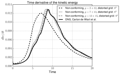
Figure 2: Evolution of the time derivative of the kinetic energy for the Taylor–Green vortex at $Re=1,600$, $M=0.05$.

5.3 Flow around a sphere at $Re=2,000$

In this section, we test our implementation within a more complicated setting represented by the flow around a sphere at $Re=2,000$ and $M=0.05$. With this value of the Reynolds number the flow is fully turbulent. In this case, a sphere of diameter $d$ is centered at the origin of the axes, and a box is respectively extended $20d$ and $60d$ upstream and downstream the direction of the flow; the box size is $30d$ in both the $x_{2}$ and $x_{3}$ directions. As boundary conditions, we consider adiabatic solid walls at the surface of the sphere [15] and far field on all faces of the box. The surface of the sphere is first triangulated using third order simplices, and a boundary layer composed of triangular prisms is extruded from the sphere surface for a total length of $3d$. The rest of the domain is meshed with an unstructured tetrahedral mesh. We then obtain an unstructured conforming hexahedral mesh by uniformly splitting each tetrahedron in four hexahedra, and each prism in three hexahedra, resulting in a total of 22,648 hexahedral elements. Figure 3 shows a zoom of the grid near the sphere. The colors indicate the solution polynomial degree used in each cell. The quality of the elements is good in the boundary layer region whereas in the other portion of the domain is fairly poor. This choice is intentional to demonstrate the performance of the algorithm on non-ideal grids.

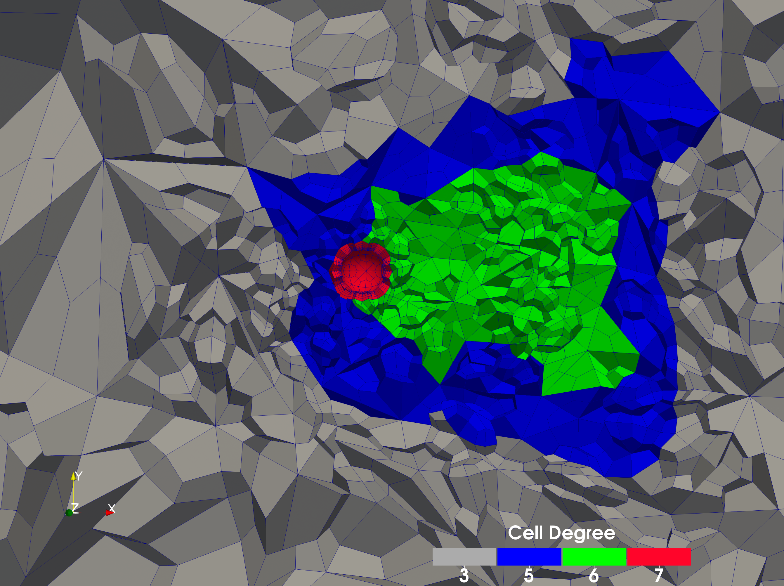
Figure 3: Polynomial order distribution for the mesh around a sphere at $Re=2,000$, $M=0.05$.

We compute the time-average value of the drag coefficient, $\langle C_{D}\rangle$, and we compare it with the value reported in in literature [64]. Figure 4, shows a time window of the evolution of the drag coefficient. To compute $\langle C_{D}\rangle$ we average the flow field and hence the aerodynamic forces for 200 time units. From Table 7, it can be seen that the computed time-average drag coefficient matches very well the value reported in literature.

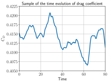
Figure 4: Sample of the evolution of the drag coefficient around a sphere at $Re=2,000$, $M=0.05$.

	$\langle C_{D}\rangle$
Munson et al. [64]	0.412
Present	0.414

Table 7: Time-average drag coefficient of a sphere at $Re=2,000$, $M=0.05$.

.

6 Conclusions

In this paper, the entropy conservative $p-$refinement/coarsening nonconforming algorithm in [45, 48] is extended to the compressible Navier–Stokes equations. The viscous terms are transformed into a quadratic form, in terms of the entropy variables, so that entropy conservation/stability of the original compressible Euler code is maintained. An LDG-IP type approach is used in discretizing the viscous terms and entropy stability of the scheme is proven. The accuracy and stability characteristics of the resulting numerical schemes are shown to be comparable to those of the original conforming scheme, in the context of the viscous shock problem, the Taylor–Green Vortex problem, and a turbulent flow past a sphere.

References

• [1] Kreiss, H.-O. and Oliger, J., “Comparison of accurate methods for the integration of hyperbolic equations,” Tellus, Vol. 24, No. 3, 1972, pp. 199–215.
• [2] Swartz, B. and Wendroff, B., “The relative efficiency of finite difference and finite element methods. I: Hyperbolic problems and splines,” SIAM Journal on Numerical Analysis, Vol. 11, No. 5, 1974, pp. 979–993.
• [3] Hutchinson, M., Heinecke, A., Pabst, H., Henry, G., Parsani, M., and Keyes, D. E., “Efficiency of High Order Spectral Element Methods on Petascale Architectures,” High Performance Computing - 31st International Conference, ISC High Performance 2016, Frankfurt, Germany, June 19-23, 2016, Proceedings, 2016, pp. 449–466.
• [4] Hadri, B., Parsani, M., Hutchinson, M., Heinecke, A., Dalcin, L., and Keyes, D., “Performance Study of Sustained Petascale Direct Numerical Simulation on Cray XC40 Systems (Trinity, Shaheen2 and Cori),” Concurrency and Computation: Practice and Experience, Vol. 0, No. 0.
• [5] Del Rey FernĂĄndez, D. C., Hicken, J. E., and Zingg, D. W., “Review of summation-by-parts operators with simultaneous approximation terms for the numerical solution of partial differential equations,” Computers & Fluids, Vol. 95, No. 22, 2014, pp. 171–196.
• [6] SvĂ€rd, M. and Nordström, J., “Review of summation-by-parts schemes for initial-boundary-value-problems,” Journal of Computational Physics, Vol. 268, No. 1, 2014, pp. 17–38.
• [7] Carpenter, M. H., Gottlieb, D., and Abarbanel, S., “Time-stable boundary conditions for finite-difference schemes solving hyperbolic systems: Methodology and application to high-order compact schemes,” Journal of Computational Physics, Vol. 111, No. 2, 1994, pp. 220–236.
• [8] Carpenter, M. H., Nordström, J., and Gottlieb, D., “A stable and conservative interface treatment of arbitrary spatial accuracy,” Journal of Computational Physics, Vol. 148, No. 2, 1999, pp. 341–365.
• [9] Nordström, J. and Carpenter, M. H., “Boundary and interface conditions for high-order finite-difference methods applied to the Euler and Navier–Stokes equations,” Journal of Computational Physics, Vol. 148, No. 2, 1999, pp. 621–645.
• [10] Nordström, J. and Carpenter, M. H., “High-order finite-difference methods, multidimensional linear problems, and curvilinear coordinates,” Journal of Computational Physics, Vol. 173, No. 1, 2001, pp. 149–174.
• [11] Carpenter, M. H., Nordström, J., and Gottlieb, D., “Revisiting and Extending Interface Penalties for Multi-domain Summation-by-Parts Operators,” Journal of Scientific Computing, Vol. 45, No. 1-3, 2010, pp. 118–150.
• [12] SvĂ€rd, M. and Özcan, H., “Entropy-stable schemes for the Euler equations with far-field and wall boundary conditions,” Journal of Scientific Computing, Vol. 58, No. 1, 2014, pp. 61–89.
• [13] Parsani, M., Carpenter, M. H., and Nielsen, E. J., “Entropy stable wall boundary conditions for the three-dimensional compressible Navier–Stokes equations,” Journal of Computational Physics, Vol. 292, No. 1, 2015, pp. 88–113.
• [14] Parsani, M., Carpenter, M. H., and Nielsen, E. J., “Entropy stable discontinuous interfaces coupling for the three-dimensional compressible Navier–Stokes equations,” Journal of Computational Physics, Vol. 290, 2015, pp. 132–138.
• [15] Dalcin, L., Rojas, D., Zampini, S., Del Rey FernĂĄndez, D. C., Carpenter, M. H., and Parsani, M., “Conservative and entropy stable solid wall boundary conditions for the compressible Navier–Stokes equations: Adiabatic wall and heat entropy transfer,” Journal of Computational Physics, Vol. 397, 2019.
• [16] Tadmor, E., “The numerical viscosity of entropy stable schemes for systems of conservation laws I,” Mathematics of Computation, Vol. 49, No. 179, July 1987, pp. 91–103.
• [17] Tadmor, E., “Entropy stability theory for difference approximations of nonlinear conservation laws and related time-dependent problems,” Acta Numerica, Vol. 12, 2003, pp. 451–512.
• [18] Fjordholm, U. S., Mishra, S., and Tadmor, E., “Arbitrarily high-order accurate entropy stable essentially nonoscillatory schemes for systems of conservation laws,” Communications in Computational Physics, Vol. 50, No. 2, 2012, pp. 554–573.
• [19] Ray, D., Chandrashekar, P., Fjordhom, U. S., and Mishra, S., “Entropy stable scheme on two-dimensional unstructured grids for Euler equations,” Communications in Computational Physics, Vol. 19, No. 5, 2016, pp. 1111–1140.
• [20] Fisher, T. C., High-order $L^{2}$ stable multi-domain finite difference method for compressible flows, Ph.D. thesis, Purdue University, August 2012.
• [21] Fisher, T. C., Carpenter, M. H., Nordström, J., and Yamaleev, N. K., “Discretely conservative finite-difference formulations for nonlinear conservation laws in split form: Theory and boundary conditions,” Journal of Computational Physics, Vol. 234, No. 1, 2013, pp. 353–375.
• [22] Fisher, T. C. and Carpenter, M. H., “High-order entropy stable finite difference schemes for nonlinear conservation laws: Finite domains,” Journal of Computational Physics, Vol. 252, 2013, pp. 518–557.
• [23] Sjörn, B. and Yee, H. C., “Adjoint error estimation and adaptive refinement for embedded-boundary Cartesian meshes,” Proceedings of ENUMATH09, Uppsala University, Sweden, 2009.
• [24] Sjörn, B. and Yee, H. C., “High order entropy conservative central schemes for wide ranges of compressible gas dynamics and MHD flows,” Journal of Computational Physics, Vol. 364, 2018, pp. 153–185.
• [25] Carpenter, M. H., Fisher, T. C., Nielsen, E. J., and Frankel, S. H., “Entropy stable spectral collocation schemes for the Navier–Stokes equations: discontinuous interfaces,” SIAM Journal on Scientific Computing, Vol. 36, No. 5, 2014, pp. B835–B867.
• [26] Winters, A. R. and J.Gassner, G., “A comparison of two entropy stable discontinuous Galerkin spectral element approximations to the shallow water equations with non-constant topography,” Journal of Computational Physics, Vol. 301, No. 1, 2015, pp. 357–376.
• [27] Parsani, M., Carpenter, M. H., Fisher, T. C., and Nielsen, E. J., “Entropy stable staggered grid discontinuous spectral collocation methods of any order for the compressible Navier–Stokes equations,” SIAM Journal on Scientific Computing, Vol. 38, No. 5, 2016, pp. A3129–A3162.
• [28] Carpenter, M. H., Parsani, M., Fisher, T. C., and Nielsen, E. J., “Towards and entropy stable spectral element framework for computational fluid dynamics,” 54th AIAA Aerospace Sciences Meeting, AIAA 2016-1058, American Institute of Aeronautics and Astronautics (AIAA), 2016.
• [29] Winters, A. R. and Gassner, G. J., “Affordable, entropy conserving and entropy stable flux functions for the ideal MHD equations,” Journal of Computational Physics, Vol. 304, No. 1, 2016, pp. 72–108.
• [30] Gassner, G. J., Winters, A. R., and Kopriva, D. A., “A well balanced and entropy conservative discontinuous Galerkin spectral element method for the shallow water equations,” Applied Mathematics and Computation, Vol. 272, No. 2, 2016, pp. 291–308.
• [31] Winters, A. R., Derigs, D., Gassner, G. J., and Walch, S., “Uniquely defined entropy stable matrix dissipation operator for high Mach number ideal MHD and compressible Euler simulations,” Journal of Computational Physics, Vol. 332, No. 1, 2017, pp. 274–289.
• [32] Chen, T. and Shu, C.-W., “Entropy stable high order discontinuous Galerkin methods with suitable quadrature rules for hyperbolic conservation laws,” Journal of Computational Physics, Vol. 345, 2017, pp. 427 – 461.
• [33] Derigs, D., Winters, A. R., J.Gassner, G., and Walch, S., “A novel averaging technique for discrete entropy-stable dissipation operators for ideal MHD,” Journal of Computational Physics, Vol. 330, No. 1, 2017, pp. 624–632.
• [34] Wintermeyer, N., Winters, A. R., Gassner, G. J., and Kopriva, D. A., “An entropy stable nodal discontinuous Galerkin method for the two dimensional shallow water equations on unstructured curvilinear meshes with discontinuous bathymetry,” Journal of Computational Physics, Vol. 340, No. 1, 2017, pp. 200–242.
• [35] Crean, J., Hicken, J. E., Del Rey FernĂĄndez, D. C., Zingg, D. W., and Carpenter, M. H., “Entropy-stable summation-by-parts discretization of the Euler equations on general curved elements,” Journal of Computational Physics, Vol. 356, 2018, pp. 410 –438.
• [36] Chan, J., “On discretely entropy conservative and entropy stable discontinuous Galerkin methods,” Journal of Computational Physics, Vol. 362, 2018, pp. 346 – 374.
• [37] Del Rey FernĂĄndez, D. C., Crean, J., Carpenter, M. H., and Hicken, J. E., “Staggered Entropy-stable summation-by-parts discretization of the Euler equations on general curved elements,” Journal of Computational Physics, Vol. 392, 2019, pp. 161–186.
• [38] Hughes, T. J. R., Franca, L. P., and Mallet, M., “A new finite element formulation for computational fluid dynamics, I: symmetric forms of the compressible Navier–Stokes equations and the second law of thermodynamics,” Computer Methods in Applied Mechanics and Engineering, Vol. 54, No. 2, 1986, pp. 223 – 234.
• [39] Friedrich, L., ShnĂŒcke, G., Winters, A. R., Del Rey FernĂĄndez, D. C., Gassner, G. J., and Carpenter, M. H., “Entropy Stable Space-Time Discontinuous Galerkin Schemes with Summation-by-Parts Property for Hyperbolic Conservation Laws,” Journal of Scientific Computing, Vol. 80, No. 1, 2019, pp. 175–222.
• [40] Ranocha, H., Sayyari, M., Dalcin, L., Parsani, M., and Ketcheson, D. I., “Relaxation Runge–Kutta Methods: Fully-Discrete Explicit Entropy-Stable Schemes for the Euler and Navier–Stokes Equations,” 05 2019, Submitted to SIAM Journal on Scientific Computing.
• [41] Olsson, P. and Oliger, J., “Energy and maximum norm estimates for nonlinear conservation laws,” Tech. Rep. 94–01, The Research Institute of Advanced Computer Science, 1994.
• [42] Gerritsen, M. and Olsson, P., “Designing an efficient solution strategy for fluid flows 1. A stable high order finite difference scheme and sharp shock resolution for the Euler equations,” Journal of Computational Physics, Vol. 129, No. 2, 1996, pp. 245–262.
• [43] Yee, H. C., Vinokur, M., and Djomehri, M. J., “Entropy Splitting and Numerical Dissipation,” Journal of Computational Physics, Vol. 162, No. 1, 2000, pp. 33–81.
• [44] Sandham, N. D., Li, Q., and Yee, H. C., “Entropy Splitting for High-Order Numerical Simulation of Compressible Turbulence,” Journal of Computational Physics, Vol. 178, No. 2, 2002, pp. 307–322.
• [45] Del Rey FernĂĄndez, D. C., Carpenter, M. H., Dalcin, L., Fredrich, L., Winters, A. R., Gassner, G. J., Zampini, S., and Parsani, M., “Entropy stable $p-$nonconforming discretizations with the summation-by-parts property for the compressible Euler equations,” Submitted SIAM Journal of Scientific Computing, 2019.
• [46] Friedrich, L., Winters, A. R., Del Rey FernĂĄndez, D. C., Gassner, G. J., Parsani, M., and Carpenter, M. H., “An entropy stable $h/p$ non-conforming discontinuous Galerkin method with the summation-by-parts property,” Journal of Scientific Computing, 2018, pp. 1–37.
• [47] Carpenter, M. H., Parsani, M., Fisher, T. C., and Nielsen, E. J., “Entropy stable staggered grid spectral collocation for the Burgers’ and compressible Navier–Stokes equations,” NASA TM-2015-218990, 2015.
• [48] Del Rey FernĂĄndez, D. C., Carpenter, M. H., Dalcin, L., Fredrich, L., Winters, A. R., Gassner, G. J., Zampini, S., and Parsani, M., “Entropy stable non-conforming discretizations with the summation-by-parts property for curvilinear coordinates,” NASA TM-2019-, 2019.
• [49] Del Rey FernĂĄndez, D. C., Boom, P. D., and Zingg, D. W., “A generalized framework for nodal first derivative summation-by-parts operators,” Journal of Computational Physics, Vol. 266, No. 1, 2014, pp. 214–239.
• [50] Vinokur, M. and Yee, H. C., “Extension of Efficient Low Dissipation High Order Schemes for $3$-D Curvilinear Moving Grids,” Frontiers of Computational Fluid Dynamics, edited by D. A. Caughey and M. Hafez, World Scientific Publishing Company, 2002, pp. 129–164.
• [51] Thomas, D. and Lombard, C. K., “Geometric Conservation Law and its application to Flow computations on moving grids,” AIAA Journal, Vol. 17, No. 10, 1979, pp. 1030–1037.
• [52] Dafermos, C. M., Hyperbolic conservation laws in continuum physics, Springer-Verlag, Berlin, 2010.
• [53] SvĂ€rd, M., “Weak Solutions and Convergent Numerical Schemes of Modified Compressible Navier–Stokes Equations,” Journal of Computational Physics, Vol. 288, No. C, May 2015, pp. 19–51.
• [54] Shi, C. and Shu, C.-W., “On local conservation of numerical methods for conservation laws,” Computers & Fluids, Vol. 169, No. 4, 2018, pp. 3–9.
• [55] Balay, S., Abhyankar, S., Adams, M. F., Brown, J., Brune, P., Buschelman, K., Dalcin, L., Dener, A., Eijkhout, V., Gropp, W. D., Karpeyev, D., Kaushik, D., Knepley, M. G., May, D. A., McInnes, L. C., Mills, R. T., Munson, T., Rupp, K., Sanan, P., Smith, B. F., Zampini, S., Zhang, H., and Zhang, H., “PETSc Users Manual,” Tech. Rep. ANL-95/11 - Revision 3.11, Argonne National Laboratory, 2019.
• [56] Knepley, M. G. and Karpeev, D. A., “Mesh Algorithms for PDE with Sieve I: Mesh Distribution,” Scientific Programming, Vol. 17, No. 3, 2009, pp. 215–230.
• [57] Abhyankar, S., Brown, J., Constantinescu, E. M., Ghosh, D., Smith, B. F., and Zhang, H., “PETSc/TS: A Modern Scalable ODE/DAE Solver Library,” arXiv preprint arXiv:1806.01437, 2018.
• [58] Dormand, J. R. and Prince, P. J., “A family of embedded Runge–Kutta formulae,” Journal of Computational and Applied Mathematics, Vol. 6, No. 1, 1980, pp. 19 – 26.
• [59] Söderlind, G., “Digital Filters in Adaptive Time-stepping,” ACM Transactions on Mathematical Software, Vol. 29, No. 1, 2003, pp. 1–26.
• [60] Söderlind, G. and Wang, L., “Adaptive time-stepping and computational stability,” Journal of Computational and Applied Mathematics, Vol. 185, No. 2, 2006, pp. 225–243.
• [61] Chandrashekar, P., “Kinetic energy preserving and entropy stable finite volume schemes for compressible Euler and Navier–Stokes equations,” Communications in Computational Physics, Vol. 14, No. 5, 2013, pp. 1252–1286.
• [62] de Wiart, C., Hillewaert, K., Duponcheel, M., and Winckelmans, G., “Assessment of a discontinuous Galerkin method for the simulation of vortical flows at high Reynolds number,” International Journal for Numerical Methods in Fluids, Vol. 74, No. 7, 2014, pp. 469–493.
• [63] Carpenter, M. H., Fisher, T. C., Nielsen, E. J., Parsani, M., SvĂ€rd, M., and Yamaleev, N., “Entropy Stable Summation-by-Parts Formulations for Computational Fluid Dynamics,” Handbook of Numerical Analysis, , No. 17, 2016, pp. 495–524.
• [64] Munson, B. R., Young, B. F., and Okiishi, T. H., Fundamental of fluid mechanics, Wiley, 2nd ed., 1990.