Landauer transport as a quasisteady state on finite chains under unitary quantum dynamics
Abstract
(Accepted in the Physical Review B - March 2020)
In this paper, we study the emergence of a Landauer transport regime from the quantum-mechanical dynamics of free electrons in a disordered tight-binding chain, which is coupled to finite leads with open boundaries. Both partitioned and partition-free initial conditions are analyzed and seen to give rise, for large enough leads, to the same spatially uniform quasi-steady-state current, which agrees with the Landauer value. The quasi-steady-state regime is preceded by a transient regime, which lasts for a time proportional to the length of the disordered sample, and followed by recursions, after a time that is proportional to the lead size. These theoretical predictions may be of interest to future experiments on transport of fermionic ultra-cold atoms across optical lattices. We also observe finite-size current oscillations, superimposed on the quasi-steady state, whose behavior depends crucially on the conditions initially imposed on the system. Finally, we show how a time-resolved Kubo formula is able to reproduce this Landauer transport regime, as the leads grow bigger.
I Introduction
The study of electronic transport is amongst the main goals of condensed matter physics. In the regime of small length scales and low temperatures, the mesoscopic transport regime, quantum coherence effects play a dominant role in the propagation of electron states. In such a case, transport can no longer be seen as a bulk phenomenon, but instead depends on device-specific details such as the geometry of and nature of the electrodes, as well as the specific distribution of disorder in the sample.
A theoretical description of mesoscopic transport was first developed by Landauer (Landauer, 1970) and later generalized by Büttiker (Büttiker, 1986). In the now called Landauer-Büttiker formalism, the problem of stationary mesoscopic transport is recast as a scattering problem, where single-electron states incoming from the leads are transmitted across a central device. The current may then be expressed as a sum over the transmission probabilities of the occupied incoming lead states. In parallel to this work, Caroli (Caroli et al., 1971) applied the non-equilibrium Green’s function formalism of Kadanoff-Baym (Kadanoff and Baym, 1962) and Keldysh (Keldysh, 1964) to the calculation of mesoscopic transport. The obtained expression has a structure similar to the Landauer-Büttiker (LB) one, but with the transmission coefficient now expressed in terms of Green’s functions of the central device and spectral functions of the leads. While apparently distinct, the two approaches lead to the same result, as implied by the Fisher-Lee relation (Fisher and Lee, 1981; Stone and Szafer, 1988; Baranger and Stone, 1989) between transmission coefficients and Green’s functions (for a detailed proof, see Wimmer (Wimmer, 2009)). Central to both approaches are the assumptions that the leads attached to the central device are semi-infinite and the occupation of the incoming single-electron states is determined by independent Fermi energies on each lead. Moreover, both methods are only able to describe steady-state transport. We also point out that the Landauer formula has also been derived within the theory of non-equilibrium steady states (Nenciu, 2007).
If one is interested in the transient dynamics and how this steady state is reached, the matter of what the initial condition of the system was, becomes relevant. At the theoretical level, two initial conditions have been historically considered: (i) In the partitioned approach (Caroli et al., 1971; Meir and Wingreen, 1992; Jauho et al., 1994), the leads and the central device are assumed to be initially disconnected, each being in equilibrium with independent Fermi levels. This Fermi-level imbalance takes into account the bias applied to the mesoscopic device. Then, the leads and the device are suddenly brought into contact allowing a charge current to flow. (ii) In the partition-free approach (Cini, 1980; Stefanucci and Almbladh, 2004a; Odashima and Lewenkopf, 2017), the leads and the device are assumed to be connected from the beginning and in global equilibrium with a common Fermi energy. Then, a potential bias between the leads is suddenly applied to the connected system. It has been shown, for the case of a single-level central device, that the same steady-state current is reached in both approaches, for the same time-dependent perturbation (Stefanucci and Almbladh, 2004a). Furthermore, the value of the steady-state current does not depend on the history of the time-dependent perturbation, provided it reaches the same constant value in the future. Crucial to this result is the fact that the leads have a continuum spectrum (as it occurs for semi-infinite leads), which allows a loss of memory about the initial conditions, provided there are no bound states in the central device. The existence of bound states inside the device is known to cause persistent current oscillations (Khosravi et al., 2008, 2009; Cornean et al., 2014a). We also point out that, under certain circumstances, interactions might prevent the formation of a steady state (Khosravi et al., 2009). Finally, the equivalence of the steady-state current reached in the partitioned and partition-free cases was shown, with rather broad assumptions and including the presence of interactions, in a mathematically rigorous way in Refs.(Moldoveanu et al., 2011; Cornean et al., 2012, 2014b).
Very recently, Purkayastha et al (Purkayastha, 2019) also discussed the problem of relating the linear response theory in a general interacting system coupled infinite leads to the open system’s Kubo formula. The authors looked at the asymptotic behavior of the integrated current-current correlators at different times, in the limit of very large systems and times. This way, they found a surprising disagreement between the transport classification given by both approaches (Purkayastha et al., 2018) for the critical one-dimensional Aubry-André-Harper model. This was attributed to the non-commutativity of the two referred limits. Nevertheless, their analysis was always done in a partitioned setup and in linear response theory.
In more recent years, a significant effort was devoted to the study of time-dependent transport and transient dynamics in mesoscopic systems attached to infinite leads (Jauho et al., 1994; Stefanucci and Almbladh, 2004b; Tuovinen et al., 2013, 2014; Latini et al., 2014; Popescu and Croy, 2016, 2017). However, the investigation of time-dependent transport in systems where the leads are finite (but possibly very large) has received much less attention. Initial work on this problem was made in Refs. (Ventra and Todorov, 2004; Bushong et al., 2005; Chien et al., 2012), in which a micro-canonical method was developed to deal with quasi-steady-state transport in finite systems, where the leads are initially connected to the device, but one of them is partially or fully depleted of particles. More recently, the same problem was considered in Pal et al (Pal et al., 2018), which studied time-dependent transport through a quantum dot connected to two systems with a quasi-continuum spectrum (discrete, but dense), which take the role of finite leads, in the partitioned approach. In all of these works, it was observed that after the transients died out, a quasisteady state transport regime emerges. However, the dependence of the quasisteady state on the system initial condition has never been explored so far. Is the quasi-steady-state current independent of the initial preparation of the system? Does the manner in which the quasisteady state is reached depend on these initial conditions? These are the questions we try to answer in this work. Notice that these issues are not of mere theoretical interest. It is true that for realistic electronic devices, consideration of finite leads is somewhat artificial.111Unless one is interested in times comparable to the discharge time of a battery, the electrodes and voltage source that are connected to a mesoscopic device can be seen as infinite. However, cold atoms trapped in optical lattices have emerged as a platform for the experimental study of transport properties (Ott et al., 2004; Rom et al., 2006) [also studied theoretically in Chien et al. (Chien et al., 2012)]. In these systems, due to the limited sizes of optical lattices, the “leads” are necessarily finite. Furthermore, while in realistic low-dimensional electronic devices, one expects electron-electron interactions play a significant role (Todorov, 2002; Bushong et al., 2005; Kurth et al., 2010; Latini et al., 2014; Cornean et al., 2014b), in optical lattices the inter-particle interaction can be tuned down to zero, thus enabling a proper study of transport for non-interacting fermions (Ott et al., 2004; Rom et al., 2006). As such, we expect that our theoretical results will be of experimental relevance for transport in ultra-cold-atoms setups.
The purpose of this work is to further explore how a steady-state transport regime emerges from quantum time-evolution in non-interacting, fermionic systems with finite, but large leads, and how the initial state of the system affects this process. By combining numerical and analytical work, we study the time-dependent current dynamics in a prototypical one-dimensional non-interacting tight-binding model with disorder, analyzing in detail how the current dynamics depends on the initial conditions (partitioned vs partition-free) and on the size of the finite leads. We employ a full quantum time evolution, starting from both initial conditions, to study the time-dependent current upon the sudden connection of the appropriate perturbation. For the partition-free case, we also derive a time-dependent Kubo formula, which allows us to see rigorously how a linear Landauer-Büttiker formula, involving only quantum transmittances, emerges from an unitary time evolution in the limit of very large leads.
The text is organized as follows. In Sec. II, we introduce the one-dimensional tight-binding model Hamiltonian that will be used throughout the rest of the paper and detail both the partitioned and partition-free approaches. In Sec. III, we describe the numerical methods used for calculating the time-dependent local current from the unitary dynamics of the finite system and also the steady-state Landauer current for infinite leads. The main numerical results are then presented in Sec. IV, where the time-evolution of the non-equilibrium current is systematically analyzed as a function of the bias, the size of the finite leads, and the central sample’s disorder and size. Finally, in Sec. V, we provide analytical insight into the numerical results of Sec. IV, by developing a time-dependent Kubo formula for the partition-free approach and expressing it in terms of complex reflection and transmission coefficients of the central sample. In Sec. VI, we discuss the obtained results and conclude the paper.
II Model Hamiltonian and initial conditions
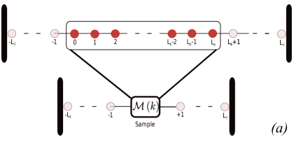
We will study the current dynamics of non-interacting electrons in a finite one-dimensional tight-binding model, with nearest-neighbor hoppings. The tight-binding chain is composed by a total of sites, with the central sites, the sample, having an on-site Anderson disorder and being subject to a constant electric field. The sites outside the sample region form the left and right leads [each with sites], are not disordered and hold a constant electrostatic potential. They will refer to the different regions in the chain as left lead (LL), sample (S), and right lead (RL). An illustrative scheme of this setup is shown in Fig. 1. For times , the dynamics of the system is governed by the time-independent Hamiltonian
| (1) |
where are creation (annihilation) operators for an electron at the chain site , is the nearest-neighbor hopping amplitude, is the fundamental charge and is the electrostatic potential. According to the previous dis-
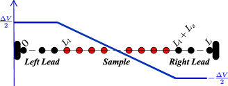
-cussion has the form
| (2) |
where is the applied potential bias, and is the Anderson on-site potential disorder, which is only present in the sample sites, and are taken as random numbers uniformly distributed inside .
We will study the current dynamics in this system both in the partitioned and partition-free approaches. In both cases, the dynamics for are governed by the Hamiltonian of Eq. (1), with only the initial state being different.
In the partitioned approach, the initial state is formed by occupied states for the partitioned system, with the bias already applied. The partitioned system is described by the Hamiltonian,
| (3) |
with , , and the Hamiltonians, respectively, for the decoupled left lead, sample, and right lead, to wit
| (4) | ||||
| (5) | ||||
| (6) |
The initial occupation of the single-electron states is determined by the independent Fermi levels for each region. Hence, we write , and , as the chemical potential for the left lead, central sample, and right lead, respectively. is a reference chemical potential. The initial state is thus described by the reduced density matrix
| (7) |
where are the independent single-electron eigenstates of the initial partitioned Hamiltonian belonging to region , , with an energy . At any temperature, the initial occupation of the states is given by the factor , with and being the Fermi-Dirac distribution function. Throughout this work, we will restrict ourselves to the case, where and being the usual Heaviside step function. The hoppings between the leads and the sample are then suddenly switched on and the time evolution of these states is generated by the Hamiltonian in Eq. (1).
In the partition-free approach, the contact between the sample and the leads is already established in the initial state, but the bias is not yet applied. Therefore, the initial condition is determined by populating the eigenstates of the partition-free Hamiltonian
| (8) |
up to a commonly defined Fermi energy, . This initial state is thus described by the reduced density matrix
| (9) |
with being eigenstates of Eq. (8) with an eigenenergy . The initial occupation factor of the states is similarly given by . In this case, the sudden perturbation driving the current is the connection of the bias potential, , at , after which the time evolution is governed by the Hamiltonian of Eq. (1).
We end this section, by noting that the charge current flowing from site to site , for the Hamiltonian of Eq. (1), is given by
| (10) |
III Numerical methods for current evaluation
III.1 Time-resolved current from quantum evolution of eigenstates
The dynamics of the system, in the partitioned approach after suddenly switching on the lead-sample hoppings, or in the partition-free approach after suddenly switching on the external bias, is governed by the Hamiltonian (1). Therefore, in both approaches and for , the reduced density matrix of the system evolves according to
| (11) |
The solution for this equation, with initial condition given by either Eq. (7) or (9), is given by
| (12) |
with the single-electron states evolving according to Eq. (1): , with being the single-electron eigenstates of either or (with occupation ), for the partitioned and partition-free approaches, respectively.
The expected value of the current, as a function of time, is given by
| (13) |
where represents the state localized at site . We also used the fact that at , for initially occupied states and for empty states. The above expression, allows us to evaluate the current flowing from site to site provided we know the time evolution of the initial single-electron states. Although correct, Eq. (13) is not very convenient from a numerical point of view, since for each initially occupied state, we would have to perform one time-evolution. A more convenient expression is obtained by writing , such that instead of evolving the initial eigenstate forwards in time, we evolve the localize states backwards in time.222Note that, despite being an evolution for negative times, the time-evolution operator used to do it is the one which includes the external perturbation: lead-sample hopping in the partitioned approach, and bias in the partition-free approach.
The current can therefore be expressed as
| (14) |
Despite being equivalent to Eq. (13), this last expression allows for a great gain in computational efficiency, as the the number of required time evolutions is reduced from to only two, for each single-time calculation of the current between sites and .
Numerically, the time-evolution of the localized states , for very large chains, is computed efficiently using a polynomial Chebyshev expansion (Tal-Ezer and Kosloff, 1984; Fehske et al., 2009) of the time evolution operator (for details, see Appendix A). Finally, the single-electron eigenstates of were calculated “on the fly” using a memory-efficient algorithm developed by Fernando (Fernando, 1997).
III.2 Landauer-Büttiker formula for the steady-state current
In Sec. IV, the time-resolved current across the sample with finite leads, calculated using the quantum evolution of the occupied states, will be compared with the steady-state value for the current as given by the Landauer-Büttiker formula for the same sample attached to infinite leads. We evaluate this current using the Caroli-Meir-Wingreen form of the Landauer-Büttiker formula (Caroli et al., 1971; Meir and Wingreen, 1992), which for a two-terminal device, at zero temperature, reads as
| (15) |
where the energy dependent transmission function is expressed in terms of Green’s functions as
| (16) |
where are real-space spectral functions of the unattached leads and are the real-space retarded/advanced Green’s function of the central sample, in the presence of the leads. For our particular one-dimensional model, the leads’ spectral functions are matrices with the only non-zero elements between boundary sites, i.e., and , where . The functions are surface density of states of the leads which may be computed analytically yielding:
| (17) |
Therefore, the final form for the transmission function reads
| (18) |
For each central sample, the retarded Green’s function in Eq. (18) was calculated by using the well-known recursive Green’s function method (MacKinnon, 1985; Wimmer, 2009; Lewenkopf and Mucciolo, 2013), using the surface Green function of the semi-infinite one-dimensional leads as boundary conditions, as detailed in Appendix B.
IV Numerical results and comparison with the Landauer formula
We evaluated the time-dependent current in finite open chains, using the method described in Sec. III.1, for both clean and disordered samples and considering both the partitioned and partition-free initial conditions. This current was then compared with the Landauer expression for the steady-state current flowing through the same sample attached to infinite leads, as described in Sec. III.2.
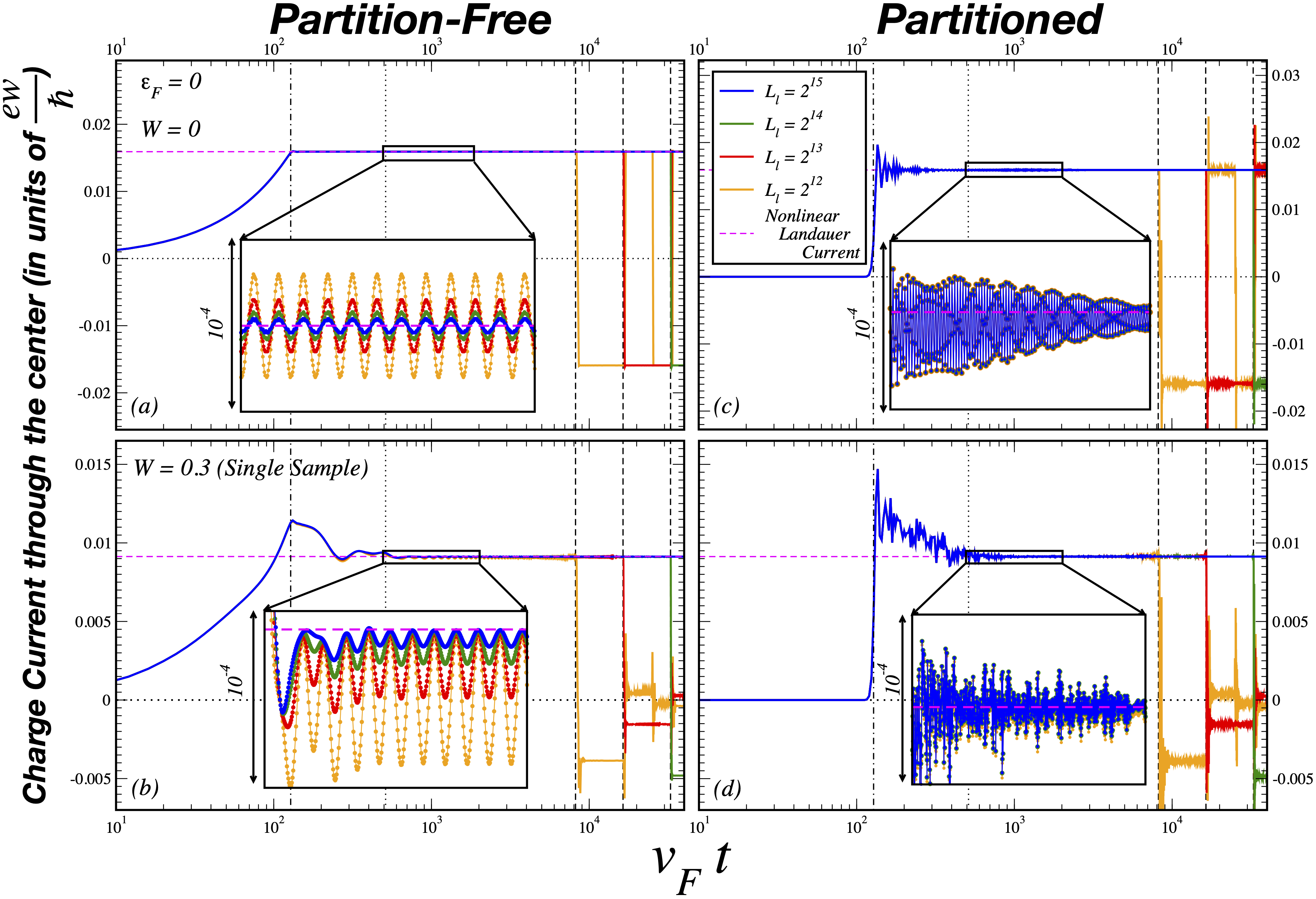
Our results are summarized in Fig. (2). For both initial conditions, three transport regimes are clearly distinguished for large enough leads: (i) initially, we have a transient regime up to a time , after which (ii) the current tends to an approximately constant quasi-steady-state value, which last up to (iii) a recurrence time, , after which an inversion of the current occurs. These three transport regimes have been previously reported for non-interacting fermions in systems with finite leads, in Refs. (Bushong et al., 2005; Chien et al., 2012), with an initial state where the leads are connected to the device, but one of the leads is depleted. These transport regimes have also been observed for interacting fermions (at a TDDFT-ALDA level) with finite leads by Bushong et al (Bushong et al., 2005). These three regimes have also been discussed in Di Ventra et al (Ventra and Todorov, 2004) and Pal et al (Pal et al., 2018). However, to the best of our knowledge the effect of different initial conditions, in each of the transport regimes has never been explored.
In the following, we will analyze in detail each of these regimes, analyzing how the different time-scales depend on the variables of the problem.
IV.1 Transient Behavior and Stabilization Times
As one could expect, the transient behavior depends on the initial preparation of the system, being different for the partitioned and partition-free approaches, as evident in Fig. 2.
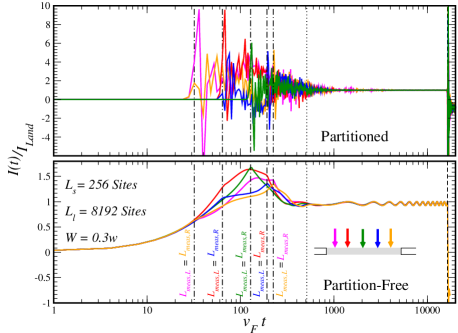
In the partitioned case, as can be seen in Figs. 2 (and also in Figs. 3 and 4), the current is initially close to zero up to a build-up time, , after which the current dramatically increases, overshooting the Landauer current value. We interpret as the time it takes for a fermion close to the initial reference Fermi level, , to travel from the lead-sample boundaries to the hopping where the current is being probed. We will define and as the distance from the point where the current is being measured in the sample to the left and right lead boundaries, respectively. We will refer to the smallest of these distances as . According to this interpretation, the build-up time is given by where is the velocity of a state initially at the reference Fermi level (the initial Fermi level defined for the sample, for the partitioned case, and the initial global Fermi level in the partition-free case). In Fig. 3, we show the current for different samples, measured at . The dashed-dotted vertical lines in Figs. 2 and 3 indicate the time . The coincidence of these lines with the
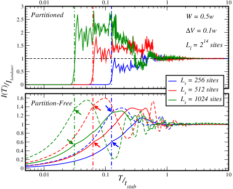
sharp rise of the current confirms our interpretation. This is further confirmed in the top panel of Fig. 4, where the current measured at different sites is shown as a function of time, with the dash-dotted vertical lines indicating the times . Once again, we can see that the current in the partitioned case is nearly zero up to the .
In the partition-free setup one observes a gradual increase of the current from the beginning. As can be seen in the bottom panel of Fig. 3, the time it takes for a fermion to travel to the current measuring position, , also marks shoulders in the current (marked by the arrows), a much weaker effect than in the partitioned case. As a matter of fact, in the partition-free case weak features (inflection points or peaks) in the current can be observed at both times and as is shown in the bottom panel of Fig. 4.
After this initial build-up, in both approaches, the current enters a sample-specific damped oscillatory phase which stabilizes towards an approximately time-independent value. This stabilization marks the beginning of the quasi-steady-state regime. As indicated in Fig. 2 and shown by the collapse of the curves in Fig. 3, for different sample sizes, the quasisteady state exists for times roughly greater than a stabilization time . Physically, this time can be interpreted as the one needed for a fermion near the initial reference Fermi level to make a round trip inside the central sample, thus probing the existing disorder landscape. The fact that both and are ballistic times (i.e., and , respectively) is consistent with the fact that we are always working in the ballistic regime of the mesoscopic central sample. Interestingly, this time-scale is nearly independent of the particular disorder configuration and the applied bias .
IV.2 Landauer Quasisteady state transport, finite-size effects and recurrence times
In both approaches, if the leads are large enough, after the initial build-up and stabilization of the current, a quasisteady state is reached for , during which the current is approximately time independent. As the size of the leads increases, the value of this quasi-steady-state current tends to the sample-specific Landauer value, independently of the initial preparation of the system (partitioned or partition-free). Hence, the present results are numerical checks to an extension of the memory-loss theorem of Stefanucci et al. (Stefanucci and Almbladh, 2004a) for the case of finite leads. The memory-loss theorem (Stefanucci and Almbladh, 2004a) states that, provided the leads have a continuum spectrum, a steady-state value of the current is achieved in the limit, and that this value is independent of the initial state of the system.
As can be seen in Figs. 2 and 5, in our case, and due to the finite nature of the leads, which makes their spectrum discrete, a quasi-steady-state only exists in a finite window of time: . For , we observe a drop and inversion of the current. Similar behavior has also been observed previously Bushong et al. (2005); Chien et al. (2012). Pal et al (Pal et al., 2018) pointed out that the recurrence time, is inversely proportional to the level spacing of the leads’ spectra, which measures how close the finite leads are to a true continuous spectrum. Our results allow for an alternative interpretation. As demonstrated in Figs. 2 — where we show the current for fixed Fermi energy and different sizes of the leads — and in Fig. 5 — where we show the current for fixed but different Fermi energies — the recurrence time is roughly given by , where is the Fermi velocity. Notice that is just the time a fermion close to the Fermi level takes to perform a round trip inside of a lead, in agreement with what was previously reported in Ref. (Bushong et al., 2005). Furthermore, one also sees that the recursion time is roughly independent of the disorder on the sample, which is consistent with its previous physical interpretation.
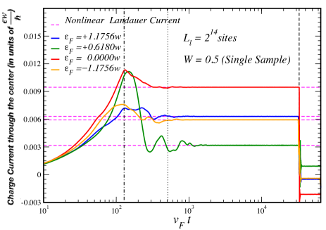
One expects that, for sufficiently large leads, the value of the current in the quasi-steady-state should approach the Landauer value, possibly with some small oscillations superimposed due to finite size effects that vanish with increasing lead size. Indeed, this is what we observe in Fig. 2. However, the way in which the oscillations vanish depends crucially on the initial condition of the system. In the partition-free approach, we observe that the current in the quasi-steady-state regime does not strictly approaches the Landauer value. Instead, there is a small persistent oscillatory component with a constant amplitude in time, superposed on its steady-state value, and which persists up to the recursion time . Although constant throughout the quasi-steady-state regime, the amplitude of these oscillations is seen to decrease as , and the value of the quasi-steady-state current approaches the Landauer value in a nearly uniform way for . We also observed, that the period of these oscillations is roughly inversely proportional to the applied bias, i.e., , but does not depend on either or . Such dependence of the oscillation period with the applied bias had also been reported by Kurth et al (Kurth et al., 2005), although their focus is on systems with infinite leads. Nevertheless, this behavior gives a hint on the physical origin of these oscillations. If we consider an occupied eigenstate of , having energy , this can always be written as a linear combination of eigenstates of . This way, its time-evolved ket, , is simply
| (19) |
where are the wave-function overlaps. Since the leads are much larger than the central sample and the effect of applying a bias is to globally shift the energy of all Wannier states in the leads to , it is reasonable to say that the two dominant overlaps in Eq. (19) will be with the states with energies . This follows from the fact that these two are precisely the ones whose real-space wave-functions in either the right or left lead are stationary waves with the same wavelength as the original one. Assuming this argument to be true, we may neglect all the other overlaps in Eq. (19) and write
| (20) |
which behaves as a two level system, with a Bohr frequency . This argument justifies the presence of the time scale associated to the period of the observed finite-size oscillations. Furthermore, as is reduced, we expect that the overlaps will increase, thus, we also expect that the amplitude of these oscillations will increase when decreases, a point to which we will return.
For the partitioned approach, a rather different behavior is observed. In this setup, as can be seen in the insets of Figs. 2 (c) and (d), the amplitude of the oscillations in the quasi-steady-state decays as time increases, provided . Furthermore, the amplitude of the oscillations is nearly independent of the leads’ size at any fixed observation time (provided for the compared lead sizes). As increases, also increases and therefore, the oscillations in the quasi-steady-state will decay for a longer time, thus tending towards the Landauer value as time tends to . Note that the physical argument given above in Eqs. (19) and (20), justifies why one does not observe persistent oscillations when the system begins in a partitioned setup.
In a true steady state, the value of the current is not only time independent but must also be position independent, as no charge accumulation can occur. Hence, we also investigated whether or not this emergent quasisteady state current in finite chains is homogeneous over the sample. Indeed, we found out that in the quasisteady state the current is approximately homogeneous in space, independently of the initial preparation of the system, for large enough leads and provided we are far away from the chain’s open extremities. This observation is exemplified in Fig. 4, where we show the time-dependent current for a disordered central sample, measured at three different bonds: center, left, and right boundaries of a randomly picked disordered sample. As can be seen, after the disappearance of the initial transients, the same quasi-steady-state current is reached at the three positions, apart from the finite-size oscillations which are out of phase.
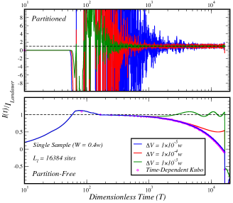
Interestingly, the establishment of a well-defined quasisteady state, for a large but fixed leads size, might not occur for very small biases, where we would expect linear response theory to hold, depending on the initial conditions. This is illustrated in Fig. 6. There, we can see that for the partition-free setup, no clear quasi-steady-state is observed for very small biases. This occurs because, for a fixed lead size and as previously explained, the period and amplitude (relative to the infinite leads’ Landauer value) of the finite-size oscillations increases with the reduction of the applied bias. Therefore, for small enough bias, the period of the oscillations might become larger than the recursion time, and no quasi-steady-state is observed. A well developed quasi-steady current only emerges provided . In the partitioned setup, the situation is a bit different and for large times: the current always tends to the Landauer value with the amplitude of the finite-size oscillations decreasing over time. These observations seem to be in agreement with the interpretation of Bushong et al. (Bushong et al., 2005), where it is put forward that the observation of a quasi-steady-state requires the change in the initial spread of the electrons’ momenta. In this reference, this occurs either due to a geometrical constriction at the lead-sample contact, or due to an initial applied energy barrier. In our case, it seems that the applied bias is the mechanism by which electrons change their initial momenta. As a general “rule-of-thumb”, we can tell that, in order to observe a quasi-steady-state current regime with minor finite-size effects, one must always consider biases that are much larger than the level spacing of the whole system’s spectrum.
IV.3 Sample-Specific Curves at Large Biases
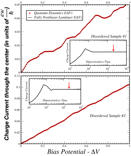
We finally point out, that the coincidence between the Landauer value for the current and the value of the current in the quasisteady state occurs for any value of the bias potential, as long as it is smaller than the bandwidth and provided a quasisteady state is established.
This is illustrated in Fig. 7, where we show values for the time-dependent current in the quasisteady state regime as a function of the applied bias, for two random disordered samples, and compare the results with the value of the Landauer current. The results clearly confirm that the quasisteady state current seen in the quantum dynamics calculations with finite leads indeed corresponds to the Landauer transport predicted for samples coupled to semi-infinite leads. The agreement between the two approaches was seen to be perfect for all the range of bias tested and well beyond linear response.
V Emergence of Landauer transport within linear response in the partition-free approach
The numerical studies of the previous section show that a quasi-steady-state transport regime, with an approximately uniform and time-independent current, emerges across finite systems subjected to a potential bias and coupled to finite but large leads. Moreover, the results also show that for large enough leads, the value of this quasi-steady-state current coincides with the Landauer result for the transport’s steady state with semi-infinite leads. In this section, we will try to shed further light on these numerical results using a semi-analytical procedure. In order to make as much analytical progress as possible, we shall restrict ourselves to the partition-free case and small biases, such that we can study the current using Kubo linear response theory in the applied bias, .
V.1 Time-dependent Kubo formula for a sudden connection
We will always consider the partition-free Hamiltonian at as the unperturbed Hamiltonian for this case, i.e.,
| (21) |
and treat the applied potential bias as the current-driving perturbation,
| (22) |
with the electrostatic potential profile, , given by Eq. (2).
In order to derive a time-dependent Kubo formula for the current, we will start by writing the equation of motion for the reduced density matrix, Eq. (11), in the eigenbasis of the unperturbed Hamiltonian. Thus, we obtain
| (23) |
where and is an eigenstate of with energy . Within linear response theory, we write the reduced density matrix as
| (24) |
where is the initial equilibrium reduced density matrix and is a small correction, which in linear response is assumed to be . Disregarding any contributions of in the equation of motion, we obtain
| (25) |
where are the matrix elements of the applied potential bias,
| (26) |
and is the amplitude of the eigenstate on site , i.e. . Now, using the fact that , it is possible to integrate Eq. (25), obtaining
| (27) |
where and . The expected value of the current that flows from site to , is thus given by
| (28) |
where we introduced
| (29) |
which are the matrix elements of the local current operator between sites and , up to a dimension-full multiplicative factor.
By further noticing that the amplitudes may be chosen as all real and is an anti-symmetric matrix, one can rewrite Eq. (28) in the following way:
| (30) |
which is our final time-dependent Kubo formula for the current.
Obviously, one cannot give a general rule for establishing the validity regime of Eq. (30), since that will depend crucially on the properties of the central disordered sample. However, for each sample, there is always a value of sufficiently small, such that a linear response theory for the current is valid. We depict such an example in the upper panel of Fig. 6, where the current traversing the central bond of a disordered sample, as obtained from Eq. (30), is compared with the one obtained from the fully nonlinear quantum dynamics of sec. III in the partition-free approach. As a further short comment on the plots of Fig. 6, it is interesting to note that, for the parameters used, it seems that no quasi-steady-state plateau emerges from the quantum dynamics close to the linear response regime. As referred before, this is simply a consequence of a greater relevance of the finite-size oscillations which, now, have a period larger than the recurrence time and a much larger relative amplitude.
V.2 Representation of the eigenstates in terms of the sample’s quantum reflection/transmission coefficients
In order to make an effective use of Eq. (30) and make analytic progress we must be able to find a semi-analytical expression for the matrix elements and , which, in principle, requires the knowledge of the eigenfunctions in the whole chain. These wave functions usually present a very complicated structure inside the disordered central sample, but for large enough leads, we actually only need to know their form in the leads. On the one hand, the matrix elements only require the knowledge of local amplitudes in the two adjacent sites across which the current is being measured. Hence, we can simply choose to measure it outside the sample. On the other hand, we expect the current to be dominated by states that are not localized in the disordered sample, but instead are delocalized in the leads. Hence, we only need to calculate the matrix elements between delocalized states. For such states, and provided the leads are much larger than the disordered sample region, we can approximate
| (31) |
This approximation, allows us to evaluate the current in the leads, without knowing the shape of the eigenwave functions inside the central sample.
Next, we notice that the form of the scattering eigenstates in the leads can be expressed in terms of the complex reflection and transmission coefficients of the central sample. For perfect leads, the wave functions of the eigenstates will have the form of a coherent superposition of left and right propagating plane-waves. With a change of notation from the previous section, we will relabel sites of the left lead with indices and the ones of the right lead with . Using this notation, the form of the eigenstate wave function in the leads have the form
| (32) |
being labeled by a crystal momentum , and with being the amplitude of a right/left propagating state in the left (right) lead. Notice that the time-independent Schrödinger equation inside the leads, still allows us to relate the crystal momentum to the energy of the state as , i.e. the same as for an infinite periodic chain. As usual in one-dimensional scattering problems, the amplitudes of propagating states on the left and right leads can be related by a transfer matrix, :
| (33) |
In the presence of time-reversal symmetry, the transfer matrix has the general form
| (34) |
where and are the moduli and phases of the transmission and reflection coefficients, respectively. Moreover, for any sample one has , which implies the conservation of current, i.e., . These coefficients are physical characteristics of the central sample only and, thus, may be rightfully calculated by assuming the leads as semi-infinite. The determination of the reflection and transmission coefficients of a specific sample, in general, can only be done numerically, using the method detailed in Appendix B. The great advantage of this method is that, once this calculation is done, the wave functions in the leads can be expressed in terms of only a few parameters. Additionally, to obtain the eigenstates, we must further impose open boundary conditions at the ends of the leads, i.e.,
| (35) |
| (36) |
where is a normalization factor, which can be determined in the limit of large leads by approximating, in the same spirit of Eq. (31),
| (37) |
This finally leads to
| (38) |
The functions and are defined as
| (39a) | ||||
| (39b) |
and where is constrained to verify the following quantization condition:
| (40) |
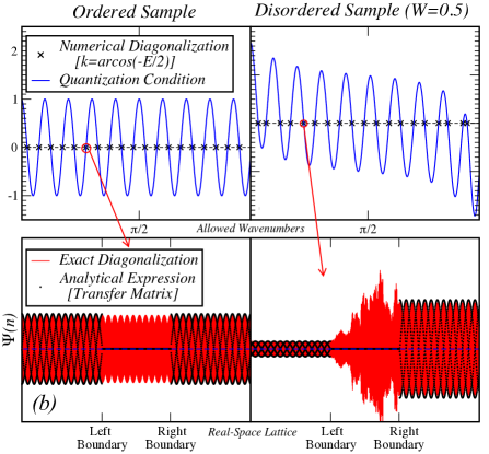
Notice that the solution of this last condition, together with the relation , allows us to determine the eigenenergies corresponding to delocalized states. In the lower panels of Fig. 8 (b), we exemplify the validity of this statement by comparing the wave functions obtained from the numerical diagonalization of , with sites, to the semi-analytical expressions of Eq. (36). The wave numbers obtained from the numerical diagonalization, i.e. , are also seen to coincide perfectly with the roots of Eq. (40) [see the upper panels of Fig. 8 (b)].
Note also that Eqs. (36) and (40) reduce to the usual result for the eigenstates of a finite open chain, when and is the phase accumulated by a plane-wave crossing the internal bonds of an ordered sample, i.e.,
| (41) |
with and . Moreover, these states are non-degenerate and also alternately symmetrical and antissymmetrical under parity (), which just reflects that same symmetry of the clean Hamiltonian.
V.3 Continuum regime of the Kubo formula
When analyzing the time-dependent Kubo formula of Eq. (30), we must take into account that there are actually two distinct time scales: (1) the observation time, , and (2) the scale associated with the spacing between the discrete energy levels of the finite chain. The latter is proportional to the length of the leads and, as discussed in the Sec. IV, is associated to the recurrence time .
As expected and confirmed in Sec. IV, the quasi-steady-state regime which approximates the Landauer transport regime of semi-infinite leads, emerges when we take (with being the time in dimensionless units), but while keeping . In such case, all the transients have died out, but the system is still far away from getting into the regime where current inversions occur. Furthermore, Eq. (30) includes a factor of , which is an emergent -function in the limit , with a broadening of in energy. This factor actually acts as a spectral filter which kills-off the contributions coming from pairs of eigenstates having an energy separation larger than . Hence, we will show in this section how the approximately time-independent quasi-steady-state current emerges, when we are in the limit , with , such that there are many eigenvalues inside the interval . We will refer to this limit as the continuum regime.
V.3.1 Approximate form of and matrices in the continuum regime
We start by noting that, in the continuum limit, since only states close to the Fermi energy contribute, it suffices to obtain the matrix elements and between states where is small and . In the limit of , the first term of Eq. (42) dominates over the second. Therefore, we can approximate it as
| (44) |
where, in the of limit , we approximated . Doing the same for , we obtain
| (45) |
where we assumed that , when approximating . This justifies why in the quasi-steady-state regime, the current is approximately uniform, if we are away from the chain’s extremities. For the current on the right lead, we obtain a similar result, namely,
| (46) |
Now, we note that for a chain without any disorder, the matrix elements of will only be non-zero if the states labeled to and have opposite parities. This selection rule stems from the fact that the fully ordered chain is symmetric under inversion and therefore its eigenstates will have a well-defined parity. Since the applied potential is an odd perturbation, it only couples states of opposite parities. In the presence of a general disorder in the central sample, we no longer have inversion symmetry. Nevertheless, one may still expect that in the limit , the breaking of the symmetry is small and an approximate selection rule should emerge. Indeed, this is the case. In order to obtain this approximate selection rule for a sample with disorder, we notice that although we can no longer classify the states as even and odd, given the quantization condition Eq. (40), which involves , we can classify the states as and according to the sign of :
| (47) |
For an ordered or symmetrically disordered sample, this reduces to a labeling of eigenstates as even or odd, respectively, under a parity transformation, . With such a classification, it can be shown (see Appendix C) that in the limits of and , one obtains the following effective selection rule:
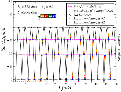
| (48) |
with and which immediately implies that , if are in the same class as . This is an approximate selection rule, analogous to the one which exists in the clean case, but which only emerges when . In Fig. 9, we represent the values of as a function of , for allowed values of and . We can clearly see that for some data points as increases, while other data points tend to a finite value, which is given by the sample-specific value, . 333As visible in Fig. 9, there is small deviation of the data points obtained for the ordered central sample from the theoretical value . These results seem incompatible with an exact parity selection rule for , for this case, however, they are not. This artifact is due to the fact that the data shown was calculated from the numerical diagonalization of and then was used to obtain the respective wave numbers. This procedure takes into account the finite dimension of the central sample and hence the allowed wave numbers are of the form , with . Since the expression of which is proportional to is only valid under an approximation which ignores [i.e. Eq. (31)], the parity selection rule appears to be approximate as well. At any rate, it may be proven, by symmetry, that this rule is actually true for any value of , if one considers the full expression for .
We point out that in the case of symmetric disorder profile, one can derive from the properties of the transfer matrix that . In this case, one immediately sees that the scattering wave functions of Eq. (36) reduce to the same form as in Eq. (41), with the parity determined by the class to which it belongs. In such a case, the factor of the and matrices comes only from this effect, since the functions and are exactly the same as in the non-disordered case. Just the allowed ’s are different.
Having established this effective selection rule, we can expand the prefactors of Eqs. (44)—(46) around . Taking into account that the only significant contributions come from pairs of states belonging to different classes, we may use Eqs. (40) and (47) to write, for ,
| (49a) | |||
| (49b) |
Using these approximations in Eq. (44), we obtain
| (50) |
and from Eqs. (45) and (46) we obtain
| (51) |
In the following, we will use Eqs. (50) and (51) to obtain the Landauer current from the Kubo formula of Eq. (30)
V.3.2 Continuum limit expression for the stationary current: Emergence of Landauer transport
Using Eqs. (50) and (51), we can write the time-dependent Kubo formula Eq. (30) as
| (52) |
where the primed sum in Eq. (52) means that only pairs of states of opposite classes are included in the sum, due to the emergent selection rule. We also introduced the quantity , which is defined as
| (53) |
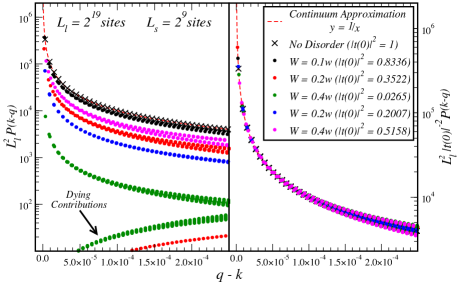
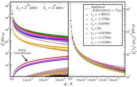
where we approximated , with . To make Eqs. (52) and (53) more clear, we remark that this definition of the current is no longer dependent on the condition , and is actually symmetrical upon exchange of the indices. The above equation also shows that, for , the latter approximately only a function of the difference in eigenenergies. This result was checked numerically as seen in Fig. 10, where we can see that for a wide variety of disordered samples and different values of the Fermi energy, all the values of [calculated directly from the wave functions in Eq. (41)] fall into the curve Eq. (53).
The time-dependent current in the continuum regime can thus be written as
| (54) |
where we introduced the joint density of contributing states (JDoCS), , as
| (55) |
The restricted summation in Eq. (55) already takes into account the emergent selection rule of Eq. (48). In Appendix D, we show that this quantity, in the limit , can be written in terms of the density of states of each class in a fully clean system and its expression for small enough is simply
| (57) |
Finally, Eq. (57) together with the facts that
| (58) |
and , yields a steady-state current
| (59) |
which is precisely the linear Landauer steady-state current for a two-terminal one-dimensional device.
Notice, that in the derivation of this result from the time-dependent Kubo formula, it is essential that with , such that the can be evaluated in the limit of , while the factor is treated as as emergent -function. When , then there will be few pairs of states with , and we can no longer treat as a -function. When this happens, we start observing recurrences in the current as reported in Sec. (IV).
VI Conclusions
In this work, we investigated how a quasi-steady-state particle transport regime emerges across disordered samples coupled to large, but finite leads which are subjected to a potential bias. In order to do so, we have studied time-dependent transport, both numerically and semi-analytically, in a non-interacting and one-dimensional tight-binding chain, with open boundary conditions, where the central region is an extended disordered sample, and the rest of the chain acts as a pair of finite, but otherwise perfect leads.
For large lead sizes, and sufficiently large bias, a quasi-steady-state regime emerges at intermediate times, after the transient behavior has died out and before inversions in the current are observed. The current in the quasi-steady-state is approximately constant in time and homogeneous in space (if measured at points far away from the chain’s extremities). Furthermore, the value of the current in the quasi-steady-state coincides with the one predicted by the Landauer formula for semi-infinite leads, independently of the initial condition of the system (partitioned or partition-free). These results amount to an exemplification and extension to finite systems of the results of Stefanucci et al (Stefanucci and Almbladh, 2004a) on the establishment of a steady-state regime of transport in samples which are attached to infinite leads.
We have found that the quasisteady state is established, for both initial conditions, after a stabilization time . Physically, this can be interpreted as the time taken by a Fermi-level state to probe the disordered landscape inside the central sample. The quasi-steady-state lasts until a recurrence time , where current inversions start happening. Aside from being related to the inverse spacing of the energy levels in the system (Pal et al., 2018), this recurrence time may also be interpreted as the time taken by a Fermi-level electron to leave the sample and return to it, by traveling back and forth inside a lead. This conclusion was seen to be independent of the central sample’s features, as long as the leads are much larger than it and transport is ballistic across the disordered sample.
During the quasi-steady-state, persistent finite-size effects are observed in the partition-free approach as superposed oscillations, with a period that is inversely proportional to the bias and an amplitude which scales to zero as but becomes more relevant (relative to ) for very small values of . This effect prevents the onset of a quasi-steady-state regime for systems prepared in the partition-free setup, if the leads are too small. In the partitioned case, the amplitude of the oscillations superposed on the quasisteady-state plateaus is not influenced by the size of leads, but instead is damped as the observation time increases (while keeping ). Similarly to the partition-free case, the amplitude of the fluctuations increases for smaller biases. These observations seem to indicate that the observation of a clear quasisteady state requires some kind of mechanism which scatters the electron’s momenta (Bushong et al., 2005). Here it is provided by the applied potential ramp in the sample, which becomes a less effective mechanism as . In both cases, these finite-size oscillations can be made arbitrarily small if is large enough.
In order to shine light on the numerical results, a time-dependent Kubo formula for the current in the partition-free approach, which is suitable for semi-analytical treatment, was developed for describing the local time-dependent current due to a small applied bias. From this formula, it was possible to see that an approximately time-independent and spatially uniform current emerges in the limit of large system’s size and observation times, , provided (in agreement with the recurrence times observed numerically). These conditions are necessary to treat the leads as being effectively infinite, in what respects DC transport. After expressing the eigenfunctions of the disordered central sample in terms of complex reflection and transmission coefficients, all the matrix elements appearing in the Kubo formula were evaluated semi-analytically. The quasi-steady-state current thus obtained was shown to reproduce the linearized Landauer formula for the current in a two-terminal device.
We hope that these theoretical predictions of the time scales over which the quasisteady state occurs and the nature of the finite-size oscillations can be experimentally tested and guide future research on mesoscopic transport in fermionic ultra-cold atomic gases in optical lattices.
VII Acknowledgments
J.M.V.P.L. and J.P.S.P. acknowledge financing of Fundação da Ciência e Tecnologia, of COMPETE 2020 program in FEDER component (European Union), through projects POCI-01-0145-FEDER-028887 and UID/FIS/04650/2013. J.P.S.P. is supported by the MAP-fis PhD grant PD/BD/142774/2018 of Fundação da Ciência e Tecnologia. B.A. acknowledges financial support from Fundação para a Ciência e a Tecnologia, Portugal, through Project Nº CEECIND/02936/2017. Additionally, J.P.S.P. also acknowledges the hospitality of the University of Central Florida, where part of this work was done, as well as Dr. Eduardo Mucciolo and Dr. Caio H. Lewenkopf for the careful reading of the manuscript and suggestions. We also thank S. M. João, Dr. Nuno M. R. Peres, Dr. Aires Ferreira and Dr. João M. B. Lopes dos Santos for enlightening discussions about this work. J.P.S.P. also acknowledges the hospitality of Katherine Vasquez during his stay in Orlando, Florida. Finally, the authors acknowledge the comments of the anonymous referees, which proved very helpful in the improvement of the original manuscript.
Appendix A Review of the recursive Chebyshev method for quantum time-evolution
In this appendix, we wish to describe shortly the algorithm used to time-evolve an arbitrary single-particle state with the full Hamiltonian. As referred in the main text, the Hamiltonian generating the time-evolution for positive times, , is time-independent and, consequently, the time-evolution operator reads
| (60) |
The method used to calculate for our systems is based on its exact expansion as a series of Chebyshev polynomials in , due to Tal-Ezer et al. (Tal-Ezer and Kosloff, 1984). Namely, one has
| (61) |
where is a dimensionless Hamiltonian, rescaled by a real parameter which guarantees that its spectrum is contained inside the interval , is the -order Chebyshev polynomial of the first-kind, is a Bessel function of the first kind and is a time measured in units of . The key to the method is to avoid the numerical diagonalization of , and instead use the recursion relation for the Chebyshev polynomials,
| (62) |
in order to evaluate all the needed , recursively. For a generic review on the application of Chebyshev spectral method to physical problems see Ref. (Weiße et al., 2006) and references within.
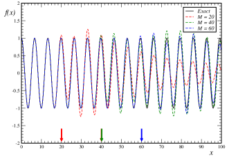
Furthermore, the Chebyshev series of Eq. (61) is known to converge rather quickly, meaning that a truncated summation with terms is usually enough to describe correctly , provided . This convergence is illustrated in Fig. 11 and in all our calculations, we used .
Notice that, in order to evaluate the current, we only require to time-evolve a given single-particle state . Therefore, we do need the full matrix form of , but instead how it acts on an arbitrary state . From the expansion of Eq. (61), we know that action to be
| (63) |
where and is the truncation order of the Chebyshev expansion. 444As this is needed in the main text, we remark that for backward time evolutions, one may simply use the fact that . Finally, the first two can be directly calculated by the simple forms of and , i.e.
| (64a) | ||||
| (64b) |
and then the remaining are efficiently calculated by using the operator generalization of the Chebyshev recursion [Eq. (62)], i.e.
| (65) |
Appendix B Review of the recursive transfer matrix method
In this appendix, we explore a very simple algorithm which allows us to calculate the transfer matrix of any given disordered sample, when it is connected to semi-infinite leads. This method is the same used in the early papers of Andereck et al (Andereck and Abrahams, 1980) and Pichard (Pichard, 1986) and allows for the calculation of with an number of operations.
For these purposes, it is more useful to re-express the Hamiltonian of the central sample in a first-quantization language, i.e.,
| (66) | ||||
where are the Wannier states of the chain and is an on-site energy (in units of the hopping ). To model the connection between the finite sample to the semi-infinite leads, one has also the following boundary hopping Hamiltonian:
| (67) |
The main purpose of this method is to find the scattering states associated to a particular disorder realization. For that, one must fix the leads’ propagating states, and , as the left and right boundary conditions for the problem. This setup is represented in Fig. 12, with the counter-propagating plane waves in the leads being represented as arrows.

B.1 Hamiltonian in Real-Space and Boundary Conditions
The first step towards the definition of the present method is expanding a scattering state (with wavenumber ) in the basis of Wannier wave functions, i.e.
| (68) |
and finally rewriting the time-independent Schrödinger equation, , in terms of the real-space amplitudes ,
| (69) |
where, by definition, outside of the sample.
As shown in Fig. 12, the boundary conditions are to be set as the plane waves defined in Eq. (32) of the main text. Reminding, one has
| (70) |
| (71) |
These states immediately set the amplitudes on the “ghost” sites of Fig. 12 to the following values:
| (72) | ||||
B.2 Review of the transfer matrix recursive method
Despite not having the look of a linear algebra problem, Eq. (69) may be turned into a matrix recursion equation, when supplemented by the trivial condition
Hence, we have
| (73) |
If we now iterate Eq. (73), we get the following relation
| (74) |
In the same way, we may write the boundary conditions of Eqs. (72), as the following matrix relations:
| (75) |
and
| (76) |
which can be inverted as
| (77) |
| (78) |
and, by definition, the transfer matrix of the whole sample is written as:
| (79) |
This last equation was the one we implemented to calculate for any given disordered sample.
Appendix C Emergence of selection rule
In this appendix, we prove the effective selection rule of Eq. (48). In order to do so, we will analyze the factor , when belong to the same or different classes. More precisely, will calculate its absolute value, which can be written as
| (80) |
where we summed and subtracted in the argument of the cosine and, then, decomposed it using the rule for the cosine of a sum of angles. The main advantage of this form is that the continuous function depends solely in the properties of the central sample and the effect of increasing the leads is to populate more densely their domains with allowed values of . This, together with the fact that we are only interested in what happens near , allows us to expand it as Taylor series on and :
| (81) |
and, consequently,
| (82) |
where the corrections are of order and disappear in the limits and . At this point, all we must do is to decompose the cosine term in Eq. (82) using the usual rules for the sum of angles and then resort to the quantization condition of Eq. (40) to realize that
| (83) |
where the sign stands for the case when and are in the same class (different classes) of states.
Finally, one can evoke the same argument as before to Taylor expand all the sample-specific functions appear in Eq. (83) [to be clear, ,,] around , but noting that by definition. Up to corrections irrelevant correction in the same limits, this gives rise to Eq. (48) of the main text after expanding the functions in powers of .
Appendix D Calculation of the joint density of contributing states
In this appendix, we will proceed to calculate the joint density of contributing states (JDoCS), for both positive and negative . For positive energy differences, , the JDoCS is defined, from Eq. (55), as
| (84) |
which may be written in terms of the usual density of states for each class, , i.e.,
| (85) |
yielding the expression,
| (86) |
in the limit of semi-infinite leads.
To progress beyond Eq. (86) in a general fashion, one starts by recognizing that, since is an intensive quantity. So these must be dominated by the states on the (clean) leads, as . Since we know that, for a clean system, the states of different parities are alternated in -space, with a regular separation given by , one concludes that
| (87) |
where is the full DoS of a clean infinite chain.
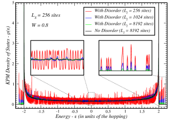
In what follows, we will always assume that the expression of Eq. (87) may be used to calculate de JDoCS in the limit of very large . This intuition is confirmed by the plots of the DoS in Fig. 13, which were obtained numerically, for a randomly selected disordered sample, using the well-known kernel polynomial method with a Jackson kernel and a fixed number of polynomials, , enough to resolve the individual energy levels in the smaller case considered (see Weiße et al. (Weiße et al., 2006) for more details on the method). Consequently, one has the following expression for the JDoCS:
| (88) |
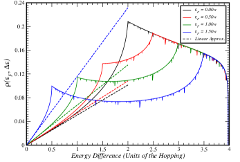
where is the Heaviside function and . The integral in Eq. (88) can be done numerically and the curves are shown in Fig. 14 for different values of the Fermi energy . Nevertheless, we are only interested in the shape of when . For that, we may expand Eq. (88) in powers of this quantity, yielding
| (89) |
Finally, we can generalize Eq. (89) to , which is trivial since, by definition [Eq. (55)], we have . Hence, our final expression is simply,
| (90) |
which is the one we use in the main text [see Eq. (56)].
References
- Landauer (1970) R. Landauer, Phil. Mag. 21, 863 (1970).
- Büttiker (1986) M. Büttiker, Phys. Rev. Lett. 57, 1761 (1986).
- Caroli et al. (1971) C. Caroli, R. Combescot, P. Nozières, and D. Saint-James, J. Phys. C: Sol. St. Phys. 4, 916 (1971).
- Kadanoff and Baym (1962) L. Kadanoff and G. Baym, Quantum Statistical Mechanics: Green’s Function Methods in Equilibrium and Nonequilibrium Problems, Frontiers in physics (Benjamin-Cummings Publishing Company, 1962).
- Keldysh (1964) L. V. Keldysh, Zh. Eksp. Teor. Fiz. 47, 1515 (1964), [Sov. Phys. JETP 20, 1018 (1965)].
- Fisher and Lee (1981) D. S. Fisher and P. A. Lee, Phys. Rev. B 23, 6851 (1981).
- Stone and Szafer (1988) A. D. Stone and A. Szafer, IBM J. Res. and Dev. 32, 384 (1988).
- Baranger and Stone (1989) H. U. Baranger and A. D. Stone, Phys. Rev. B 40, 8169 (1989).
- Wimmer (2009) M. Wimmer, Quantum transport in nanostructures: from computational concepts to spintronics in graphene and magnetic tunnel junctions, Dissertationsreihe der Fakultät für Physik der Universität Regensburg No. 5 (Univ.-Verl. Regensburg, 2009).
- Nenciu (2007) G. Nenciu, J. Math. Phys. 48, 033302 (2007).
- Meir and Wingreen (1992) Y. Meir and N. S. Wingreen, Phys. Rev. Lett. 68, 2512 (1992).
- Jauho et al. (1994) A.-P. Jauho, N. S. Wingreen, and Y. Meir, Phys. Rev. B 50, 5528 (1994).
- Cini (1980) M. Cini, Phys. Rev. B 22, 5887 (1980).
- Stefanucci and Almbladh (2004a) G. Stefanucci and C.-O. Almbladh, Phys. Rev. B 69, 195318 (2004a).
- Odashima and Lewenkopf (2017) M. M. Odashima and C. H. Lewenkopf, Phys. Rev. B 95, 104301 (2017).
- Khosravi et al. (2008) E. Khosravi, S. Kurth, G. Stefanucci, and E. K. U. Gross, Appl. Phys. A 93, 355 (2008).
- Khosravi et al. (2009) E. Khosravi, G. Stefanucci, S. Kurth, and E. K. U. Gross, Phys. Chem. Chem. Phys. 11, 4535 (2009).
- Cornean et al. (2014a) H. D. Cornean, A. Jensen, and G. Nenciu, Ann. Henri Poincaré 15, 1919 (2014a).
- Moldoveanu et al. (2011) V. Moldoveanu, H. D. Cornean, and C.-A. Pillet, Phys. Rev. B 84, 075464 (2011).
- Cornean et al. (2012) H. D. Cornean, P. Duclos, and R. Purice, Ann. Henri Poincaré 13, 827 (2012).
- Cornean et al. (2014b) H. D. Cornean, V. Moldoveanu, and C.-A. Pillet, Commun. Math. Phys. 331, 261 (2014b).
- Purkayastha (2019) A. Purkayastha, Jour. Stat. Mech. 2019, 043101 (2019).
- Purkayastha et al. (2018) A. Purkayastha, S. Sanyal, A. Dhar, and M. Kulkarni, Phys. Rev. B 97, 174206 (2018).
- Stefanucci and Almbladh (2004b) G. Stefanucci and C.-O. Almbladh, Europhysics Letters (EPL) 67, 14 (2004b).
- Tuovinen et al. (2013) R. Tuovinen, R. van Leeuwen, E. Perfetto, and G. Stefanucci, Journal of Physics: Conference Series 427, 012014 (2013).
- Tuovinen et al. (2014) R. Tuovinen, E. Perfetto, G. Stefanucci, and R. van Leeuwen, Phys. Rev. B 89, 085131 (2014).
- Latini et al. (2014) S. Latini, E. Perfetto, A.-M. Uimonen, R. van Leeuwen, and G. Stefanucci, Phys. Rev. B 89, 075306 (2014).
- Popescu and Croy (2016) B. S. Popescu and A. Croy, New J. Phys. 18, 093044 (2016).
- Popescu and Croy (2017) B. S. Popescu and A. Croy, Phys. Rev. B 95, 235433 (2017).
- Ventra and Todorov (2004) M. D. Ventra and T. N. Todorov, Jour. Phys.: Cond. Matt. 16, 8025 (2004).
- Bushong et al. (2005) N. Bushong, N. Sai, and M. Di Ventra, Nano Lett. 5, 2569 (2005).
- Chien et al. (2012) C.-C. Chien, M. Zwolak, and M. Di Ventra, Phys. Rev. A 85, 041601(R) (2012).
- Pal et al. (2018) P. P. Pal, S. Ramakrishna, and T. Seideman, The Journal of Chemical Physics 148, 144707 (2018).
- Ott et al. (2004) H. Ott, E. de Mirandes, F. Ferlaino, G. Roati, G. Modugno, and M. Inguscio, Phys. Rev. Lett. 92, 160601 (2004).
- Rom et al. (2006) T. Rom, T. Best, D. van Oosten, U. Schneider, S. Fölling, B. Paredes, and I. Bloch, Nature 444, 733 (2006).
- Todorov (2002) T. N. Todorov, Jour. Phys.: Cond. Matt. 14, 3049 (2002).
- Kurth et al. (2010) S. Kurth, G. Stefanucci, E. Khosravi, C. Verdozzi, and E. K. U. Gross, Phys. Rev. Lett. 104, 236801 (2010).
- Tal-Ezer and Kosloff (1984) H. Tal-Ezer and R. Kosloff, The Journal of Chemical Physics 81, 3967 (1984).
- Fehske et al. (2009) H. Fehske, J. Schleede, G. Schubert, G. Wellein, V. S. Filinov, and A. R. Bishop, Phys. Lett. A 373, 2182 (2009).
- Fernando (1997) K. V. Fernando, SIAM Journal on Matrix Analysis and Applications 18, 1013 (1997).
- MacKinnon (1985) A. MacKinnon, Zeitschrift für Physik B Condensed Matter 59, 385 (1985).
- Lewenkopf and Mucciolo (2013) C. H. Lewenkopf and E. R. Mucciolo, J. Comput. Electron. 12, 203 (2013).
- Kurth et al. (2005) S. Kurth, G. Stefanucci, C.-O. Almbladh, A. Rubio, and E. K. U. Gross, Phys. Rev. B 72, 035308 (2005).
- Weiße et al. (2006) A. Weiße, G. Wellein, A. Alvermann, and H. Fehske, Rev. Mod. Phys. 78, 275 (2006).
- Andereck and Abrahams (1980) B. S. Andereck and E. Abrahams, J. Phys. C: Solid State Phys. 13, L383 (1980).
- Pichard (1986) J. L. Pichard, J. Phys. C: Sol. St. Phys. 19, 1519 (1986).