Optimizing Nondecomposable Data Dependent Regularizers via Lagrangian Reparameterization offers Significant Performance and Efficiency Gains
Abstract
Data dependent regularization is known to benefit a wide variety of problems in machine learning. Often, these regularizers cannot be easily decomposed into a sum over a finite number of terms, e.g., a sum over individual example-wise terms. The measure, Area under the ROC curve (AUCROC) and Precision at a fixed recall (P@R) are some prominent examples that are used in many applications. We find that for most medium to large sized datasets, scalability issues severely limit our ability in leveraging the benefits of such regularizers. Importantly, the key technical impediment despite some recent progress is that, such objectives remain difficult to optimize via backpropapagation procedures. While an efficient general-purpose strategy for this problem still remains elusive, in this paper, we show that for many data-dependent nondecomposable regularizers that are relevant in applications, sizable gains in efficiency are possible with minimal code-level changes; in other words, no specialized tools or numerical schemes are needed. Our procedure involves a reparameterization followed by a partial dualization – this leads to a formulation that has provably cheap projection operators. We present a detailed analysis of runtime and convergence properties of our algorithm. On the experimental side, we show that a direct use of our scheme significantly improves the state of the art IOU measures reported for MSCOCO Stuff segmentation dataset.
1 Introduction

Data dependent regularization is a mature and effective strategy for many problems in machine learning. In semi-supervised learning Corduneanu and Jaakkola (2006), the marginal distribution of the examples may serve to influence the estimation of the conditional distribution and in SVMs, one could optimize the maximum relative margin based on the data distribution, rather than the absolute margin. In modern deep learning, data-dependent regularization is routinely used in both explicit and implict ways. A regularizer can take the form of certain geometric or clustering-type constraints Lezama et al. (2018); Zhu et al. (2018) on the representations that are learned by the network – using the distribution overlap between different classes Rippel et al. (2015) or seeking decorrelated autoencoder latent codes Cheung et al. (2014). On the other hand, artificial corruption of the data is also a form of regularization – dropout method induces a regularization on the Fisher information matrix of the samples Wager et al. (2013). More recently, the results in Mou et al. (2018) offer a nice treatment of the form of data-dependent regularization that emerges from popular methods such as batch normalization and AdaGrad.
From Decomposable to Nondecomposable data-dependent regularizers. A number of data-dependent regularizers described above can be written as a sum of individual example-wise estimates of the regularizer. This setting is desirable because in order to run a SGD type algorithm, we simply pick a random sample to get an unbiased estimate of the gradient. But a number of application domains often necessitate a regularization criteria that may not decompose in this manner. In such settings, a random sample (minibatch) of the dataset does not provide us an unbiased gradient – biased gradients are known to adversely impact both the qualitative and quantitative performance of the training procedure, see Chen and Luss .
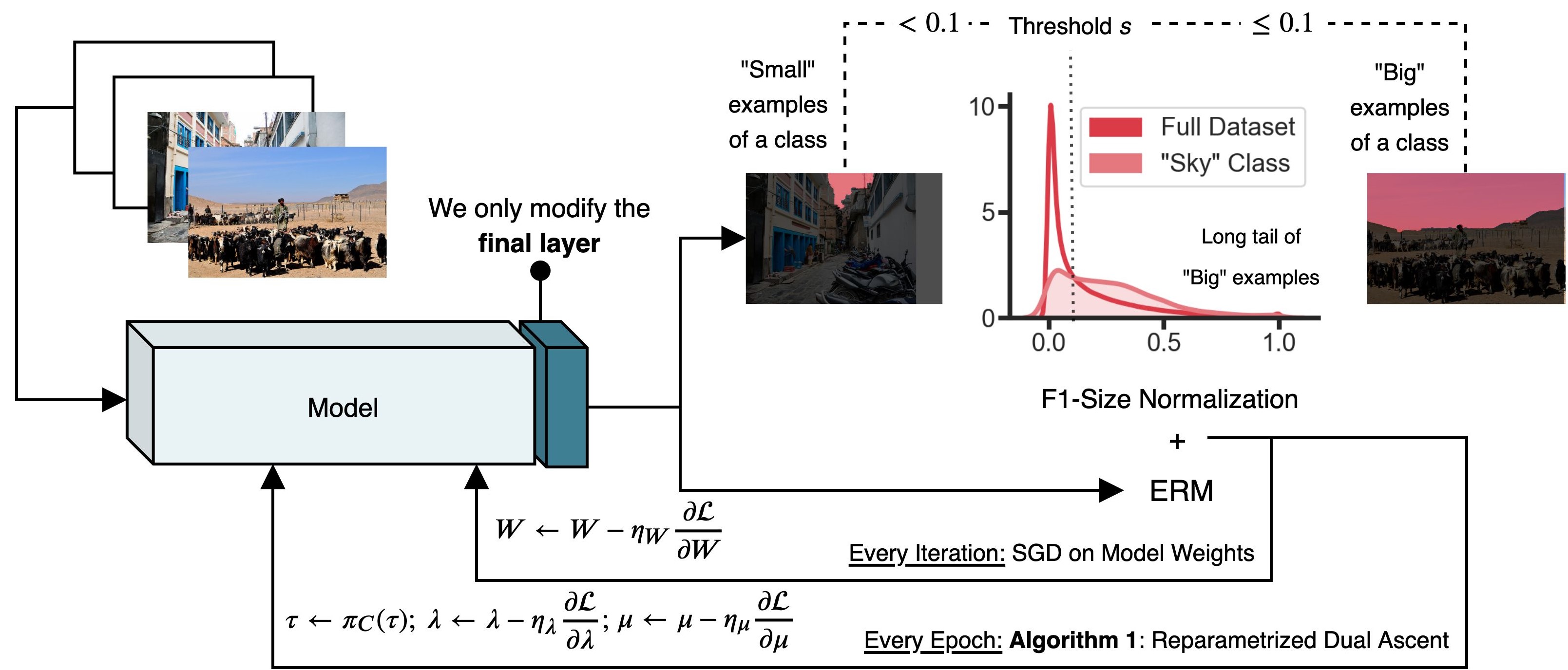
Why are Nondecomposable regularizers relevant? Consider the situation where we would like to ensure that the performance of a statistical model is uniformly good over groups induced via certain protected attributes (such as race or gender), see Figure 1. Or alternatively, we want that when updating an algorithm in a manufacturing process, the new system’s behavior should mostly remain similar with respect to some global measures such as makespan Limentani et al. (2005). Cotter et al. (2019) shows applications of various shape constraints that are associated with set functions. And finally, when pooling datasets from multiple sites, global characteristics of Precision-Recall should be (approximately) preserved across sites Zhou et al. (2017). Essentially, these applications suggest that the performane of a model in expectation (on the entire population), does not automatically guarantee that the model will perform well on specific subgroups. Motivated by these issues encountered in various real world problems, recently Cotter et al. (2018) presents a comprehensive study of the computational aspects of learning problems with rate constraints – there, the constrained setting is preferred (over penalized setting) due to several reasons including its ease of use for a practitioner. The authors show that for a general class of constraints, a proxy-Lagrangian based method must be used because the Lagrangian is not optimal. This raises the question whether there exist a broad class of data-dependent nondecomposable functions for which the regularized/penalized formulation based on standard Lagrangian schemes may, in fact, be effective and sufficient. In this paper, we will address this question with simple examples shortly.
Examples in statistics. Nondecomposable regularization, in the most general sense, has also been studied from the statistical perspective, and is often referred to as shape constraints Groeneboom and Jongbloed (2014). The need for shape constraints arise in clinical trials and cohort studies of various forms in the competing risk model, formalized using local smooth function theory, see Chapter 5 in Daimon et al. (2018) and Chenxi and Fine (2012). While several authors have studied specific forms of this problem, the literature addressing the computational aspects of estimation schemes involving such regularizers is sparse, and even for simple objectives such as a sparse additive model, we find that results have appeared only recently Yin and Yu (2018). Leveraging these ideas to train richer models of the forms that we often use in modern machine learning, establishing their convergence properties, and demonstrating their utility in real world applications is still an open problem.
Our Contributions. We first reparameterize a broad class of nondecomposable data-dependent regularizers into a form that can be efficiently optimized using first order methods. Interestingly, this reparameterization naturally leads to a Lagrangian based procedure where existing SGD based methods can be employed with little to no change, see Figure 2. While recent results suggest that optimizing nondecomposable data-dependent regularizers may be challenging Cotter et al. (2018), our development shows that a sizable subclass of such regularizers indeed admit simple solution schemes. Our overall procedure comes with convergence rate guarantees and optimal per-iteration complexity. On the MSCOCO stuff segmentation dataset, we show that a direct use of this technique yields significant improvements to the state of the art, yielding a mean IoU of 0.32. These results have been submitted to the leaderboard.
2 Preliminaries
Basic notations. We assume that the training data is given as pairs of where the joint distribution is unknown. Here, are random variables that represent examples (e.g., images) and labels respectively. We make no assumptions on and in that the marginal distributions of and can be discrete or continuous. Our goal is to estimate a function that achieves the minimum error measured using a specified loss function on the empirical/observed samples. We will use to represent the trainable parameters of a feedforward neural network with layers, with nonlinear activation functions. The output of the function computed by the neural network may be used to construct the classification or regression function .
Nondecomposability. Now, suppose there exists a function such that is a random variable called “shape” in a similar sense as described above Groeneboom and Jongbloed (2014). Our notation is suggestive of the fact that is nondecomposable, i.e., the value for individual datapoint/example may depend on the entire (empirical) distribution of . Moreover, this implies that without any further assumptions, any loss function on used to learn a model to predict cannot be represented as a decomposable function with respect to the training data , see Narasimhan et al. (2014); Sanyal et al. (2018).
As briefly noted in Section 1, nondecomposability poses unique challenges in designing algorithms for learning models with a large number of parameters. In most cases, existing backpropagation based techniques may not be directly applicable and require careful modifications Zhang et al. (2018). In other cases, they may require significant computational overhead due to expensive projection operations Kar et al. (2014). Before we present our model, we now briefly describe two fundamental tasks that are, by and large, the most frequently used modules in vision based pipelines to see the benefits of nondecomposability.
Example 1.
Object Detection seeks to simultaneously localize and classify objects in an image using a bounding box for each object Zhao et al. (2019). Naturally, since the bounding boxes are rectangular, the data-dependent regularizer is fully determined by the size of the objects. In other words, here becomes the area of the bounding box of the object. Here, we may use the knowledge of to learn that can perform equally well over all sizes present in the training data. But even though we may simply use class activation maps to compute the empirical distribution of Zhou et al. (2016), the loss functions that are commonly used are nondecomposable as we will see shortly.
Example 2.
Semantic Segmentation seeks to assign each pixel of an image to a class Chen et al. (2018). Recent works suggest that in order to train a model , we may choose a model whose complexity strongly depends on the number of pixels in the images, see Liu et al. for a recent survey. Unfortunately, these methods use up/down-sampling and so the learned representations do not directly offer immunity to variations in how much of the image is occupied by each class (i.e., size).
Remark 1
We use these two examples to illustrate the applicability of our developments – since the use case corresponds to size, we may assume that the “shape” random variable is discrete. To that end, we will use to denote the countable scoring set or the support of with .
2.1 Incorporating measures for Optimization
Let us write down a formulation which incorporates our shape regularizer. The objective function is a sum of two terms: (1) a decomposable Empirical Risk Minimization (ERM) term to learn the optimal function which maps to and (2) a nondecomposable, data dependent measure regularizer term for from . In particular, for a fixed , we seek to solve the following optimization problem,
| (1) |
where represents the empirical distribution, and with denoting training data examples. We let to be any standard loss function such as a cross entropy loss, hinge loss and so on. To keep the presentation and notations simple but nonetheless illustrate our main algorithmic developments, we will assume that the Measure is given by metric Lipton et al. while noting that the results apply directly to other measures such as R@P, P@R and can be easily generalized to other nondecomposable metrics such as AUCROC, AUCPR, using the Nyström method with no additional computational overhead Eban et al. (2016).
3 Reparameterizing Measures
Since any backpropagation based procedure can easily handle decomposable terms, let us ignore the ERM term in our objective function (1) for the moment, and focus on the second term. Specifically, in this section, we will focus on the metric as a placeholder for measures. and show that there is a reformulation which will enable a backpropagation based procedure to solve our problem (1). For simplicity, let us assume that and . The appendix shows how to extend our approach to any finite and noting that in various applications in Section 4, suffices and is already quite effective (e.g., the learned model works whether is or ).
The starting point of our technical development is the following result,
Observation 1 (Restated from Eban et al. (2016))
If is linear, i.e., , we can represent the measure term as a Linear Program (LP) as shown in equation (13) in Eban et al. (2016).
Moving forward from Observation 1. In principle, one could use standard LP solvers to solve the LP in Eban et al. (2016). But this requires instantiating the constraint matrix (linear in the number of samples). This is impractical – the alternative in Eban et al. (2016) is to use an iterative ascent method. In general this will also require a projection scheme, e.g., solving a QP. While more attractive than using an off-the-shelf method, both options may need cubic time.
Further, this discussion of the computational issues only pertains to a linear objective – the setting expectedly becomes much more challenging for non-convex objectives common in deep learning architectures.
3.1 Simplify and Reparameterize
We will first generalize the construction in Eban et al. (2016) to be more amenable to non-linear functions that one often estimates with DNN architectures. Note that since our data-dependent measures are specified on the input distribution of examples or representations derived from the transformations induced by the network , we may denote representations in general as : in other words, the th layer provides us a representation of example . We define (and similarly ) with , and , calculated using only the training data samples . We will still focus on the nondecomposable term but bring in the DNN loss when we describe the full algorithm.
Eliminating redundancy in Problem (2).
First, notice that we can eliminate the term from the objective function in (2a) since any feasible solution has to satisfy the first constraint in (2d). Second, using the definition of hinge loss, we can eliminate the terms in the objective by replacing with . This rearrangement leads to a LP in Problem (3).
Remark 3
The choice of to be the hinge loss is natural in the formulation of metric. Our Algorithm 3 can easily handle other commonly used loss functions such as Square, Cross Entropy, and Margin.
Reparameterization Via Partial Dualization.
Problem (3) has a objective which is expressed as a sum over finite number of terms. But overall, the problem remains difficult because the constraints (3b) are nonlinear and problematic. It turns out that a partial dualization – for only the problematic constraints – leads to a model with desirable properties. Let us dualize only the constraints in (3b) using , and the equality constraint in (3c) using , where and are the dual variables. This yields the Lagrangian,
| (4) |
We can denote the set . With this notation, our final optimization problem for the measure can be equivalently written as,
| (5) |
We will shortly describe some nice properties of this model.
Relation to “Disintegration”. While procedurally the derivation above is based on numerical optimization, the form in (14) is related to disintegration. Disintegration is a measure theoretic tool that allows us to rigorously define conditional probabilities Faden et al. (1985). As an application, using this technique, we can represent any (also, nondecomposable) measure defined over the graph of a convex function using (conditional) measures over its faces Caravenna and Daneri (2010). Intuitively, at the optimal solution of (14), the dual multipliers can be thought of a representation of the “disintegrated” measure, as seen in the last term in (4). In words, if we can successfully disintegrate the measure, then there exists a loss function that can be written in the weighted ERM form such that the optimal solutions of the resulting ERM and that of the nondecomposable loss coincide. But in general, Lagrangians are difficult to use for disintegration because s need not sum to one; and more importantly, when the optimal solution is in the interior of the feasible set in Prob. (3), then by complementarity slackness. This means that the decomposition provided by the s need not be a nontrivial (probability) measure in a rigorous sense.
3.2 Core benefit of Reparameterization: Efficient Projections will become possible
The previous section omitted description of any real benefits of our reparameterization. We now describe the key computational benefits.
Can we perform fast Projections? Yes, via Adaptive Thresholding.
Observe that for the formulation in (14) to offer any meaningful advantage, we should be able to show that the Lagrangian can indeed be efficiently minimized with respect to . This will crucially depend on whether we can project on to the set defined above. We now discuss that this holds for different batch sizes.
Fast projections when batch size, is . Let us denote by , the minibatch size used to solve (14) and consider the setting where we have and as used in Probs. (2)-(3). In this case, we can randomly draw a sample from and another from . Observe that only one coordinate of , namely , changes after the primal update. Hence, the projection is given by the following simple rule: after the primal update, if , we simply set leaving unchanged; on the other hand if , then we have two cases: Case (1) If , then do nothing, and Case (2) If , then set . In other words, the projection is extremely easy.
Remark 4
We can indeed use multiple samples (and take the average) to compute gradients of weights , but only update one with this scheme.
Generalizing the projection algorithm to larger batch sizes: . Note that projections onto sets defined by linear inequality constraints can be performed using standard (convex) quadratic programming solvers. But in the worst case, such solvers have a time complexity of . It is not practical to use such solvers efficiently in end-to-end training of widely used neural network architectures. It turns out that a much simpler scheme will work well.
Define , and . The Euclidean projection amounts to solving the following quadratic program:
| (6) |
Our projection algorithm to solve (9) is given in Algorithm 4 which requires only a sorting oracle. The following lemma shows the correctness of Algorithm 4.
Lemma 5
There exists an algorithm to solve (9) that requires only sorting and thresholding operations.
Proof Please see appendix.
| (7a) | ||||
| (7b) | ||||
3.3 Obtaining a numerical optimization scheme
With the results in the preceding section, we now describe below an efficient approach to solve (1).
Reparameterized Dual Ascent. Using the projection operator above (Alg. 4), our final algorithm to solve Measures regularized problem (1) is given in Algorithm 3 where we use to denote the dual step size. The following theorem characterizes the convergence rate of Algorithm 3.
Theorem 6
Assume that , and in the ERM term in Prob. (1). Then, Alg. 3 converges to a approximate (local) solution of Prob. (1) in iterations.
Proof We will use Theorem 1 in Mahdavi et al. (2012) with and , see appendix.
Remark 7
Computational Complexity. Assume that each gradient computation is , Alg. 3 requires iterations to compute a local -optimal solution (inner loop). We use a constant number of epochs (outer loop), so the total cost is . Please see supplement for more details.
Discussion. The reader will notice that the projection step in Algorithm 3 is outside the inner loop, whereas classical Lagrangian based methods guarantee convergence when the projection is performed in the inner loop. One advantage of having the projection outside the inner for loop is that SGD type methods allow for faster optimization of the Lagrangian with respect to the primal variables . That is, it is now known that constant step size policies guarantee faster convergence of the inner for loop under some structural assumptions Dieuleveut et al. (2017). In any case, we give a detailed description of our Algorithm 3 in the supplement with a discussion of the trade-off between using projections in the inner for loop versus the outer for loop in Algorithm 3.
3.4 Approximating for Backpropagation
Recall that our primary goal is to solve our optimization problem (14) using backpropagation based methods. In the previous sections, we argued that SGD can be used to solve (14). In particular, we showed in Theorem 10 that Algorithm 3 requires fewer projections compared to the classical PGD algorithm. It turns out that the simplicity of the projection operator can be exploited to avoid the double for loops in Algorithm 3, thus enabling backpropagation based training algorithms to be effectively deployed. Please see supplement for all the details.
4 Experimental Evaluations
Overview. We show experiments on three different tasks: Measures defined using the metric can be efficiently optimized using our Reparameterized Dual Ascent Algorithm 3 in large scale vision problems while strongly improving the empirical performance. The first set of experiments is designed to show that the metric based objectives may benefit existing classification models using convex classifiers. The second set of experiments further evaluates the performance of Alg. 3 for nonconvex models. Our goal here is to show that nondecomposable regularizers can be used to stabilize models without sacrificing on the overall accuracy. In the third set of experiments, we show that architectures used for Semantic Segmentation can be trained using Alg. 3. In all our experiments, we used ADAM optimizer (with default parameters) to train with primal step sizes of , and dual step sizes of , and . We report the results for the regularization parameter taking values . Baseline corresponds to .


Experiment 1) Improving Linear Classifiers using Measures
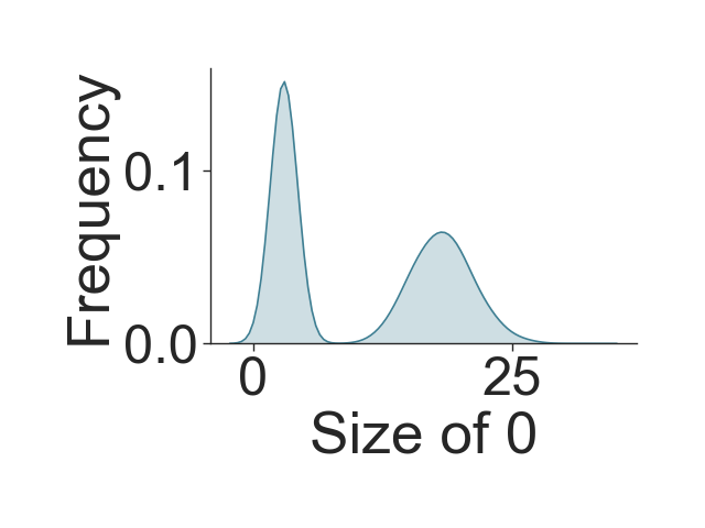
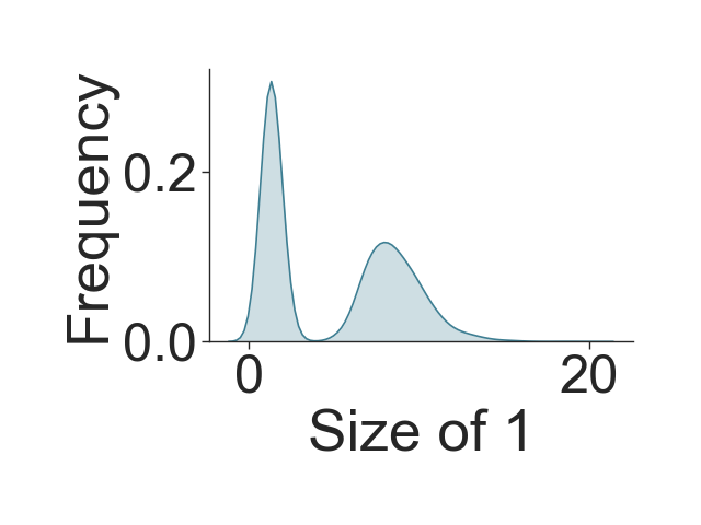
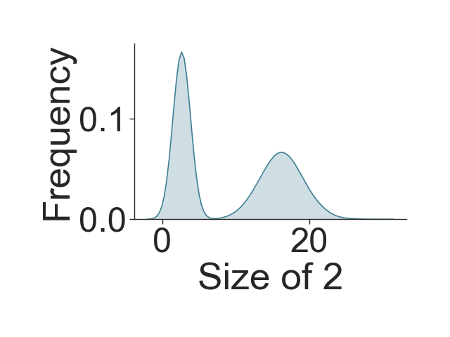
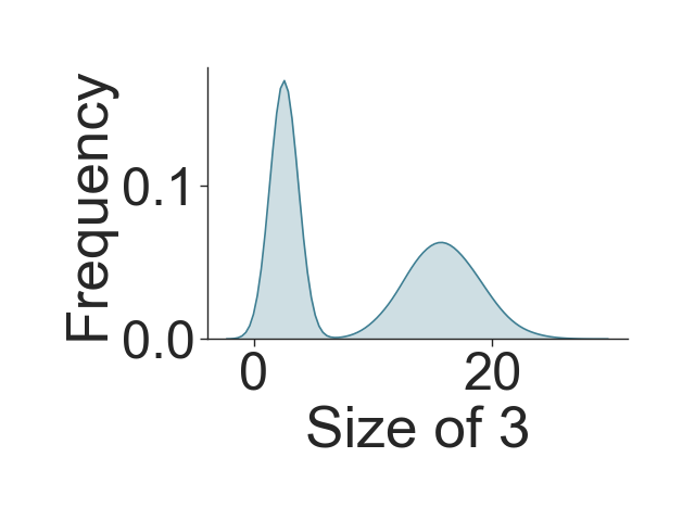
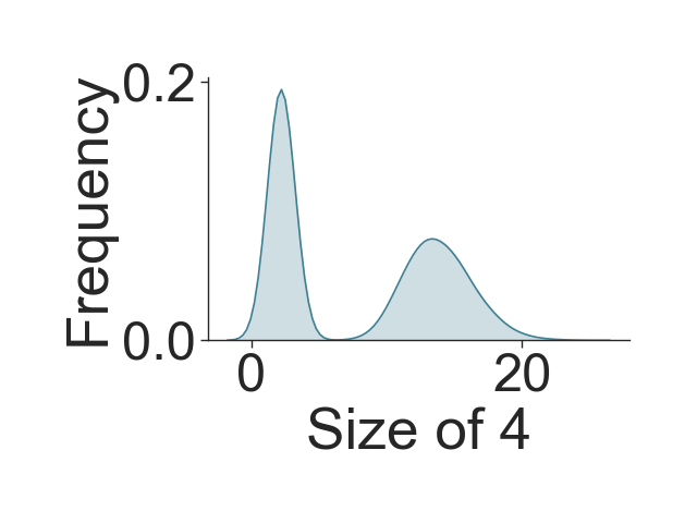
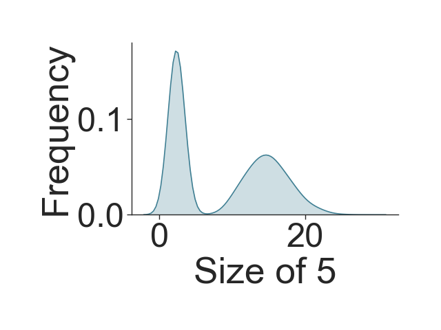
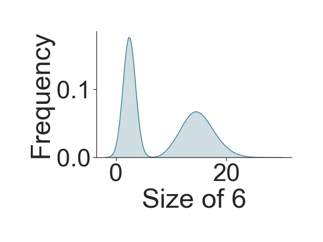
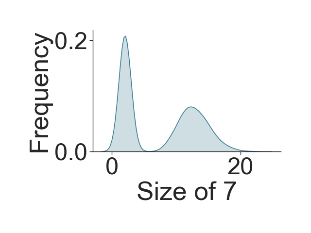
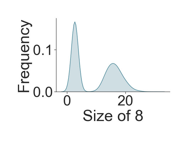
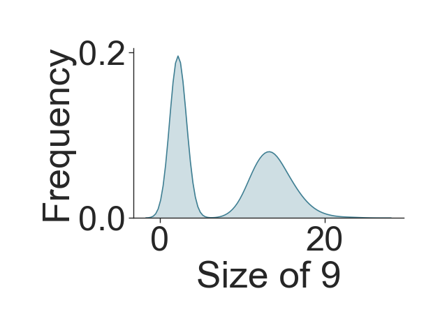
Dataset. Consider a dataset with distinct classes: MNIST with 10 classes (digits). In MNIST, the size of the foreground (pixels with nonzero intensities) is about the same for all images (and each class) in MNIST – the distribution of foreground size is unimodal (see appendix). To see the benefits of measures, we create an augmented dataset called MNIST. We added a set of images in which the foreground is double the original size in MNIST simply by rescaling the foreground to get a two mode .
How to obtain size s? To get , we can simply threshold using the empirical mean.
Model and Training. We used a single layer neural network to predict from but added an extra node to account for the Measure term in (1). That is, our total loss is the sum of the softmax cross-entropy ERM loss and the Measure (using metric). We trained using Alg. 3 for epochs with a minibatch size of .
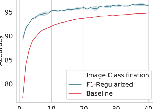
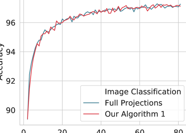
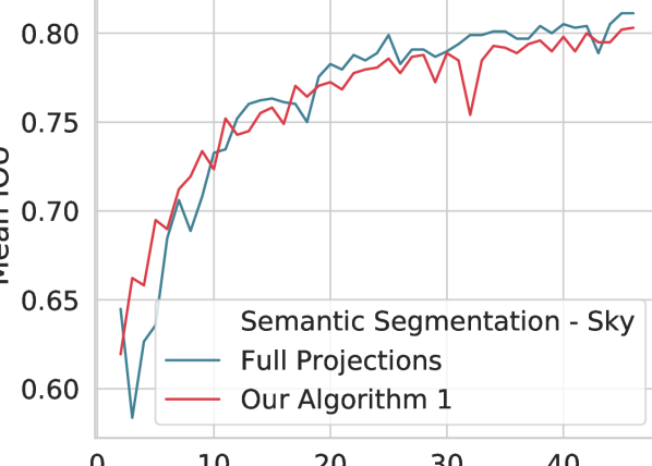
Results. We see the benefits provided by the metric as a data-dependent regularizer in Fig. 3. Column 1 shows that our model is uniformly more accurate than the baseline throughout the training process. Moreover, Column 2 compares Alg. 3 with classical dual ascent procedures from Cotter et al. (2018). Here, full projections refers to computing after every inner iteration in Alg. 3. Clearly, we can see that Algorithm 3 obtains high quality solutions but needs one projection operation every epoch.
Takeaway #1. Models obtained using Alg. 3 are more accurate and stable for linear classifiers.
Experiment 2) Improving one class Segmentation using Measures.
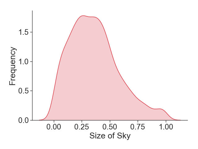
We consider the task of the pixel-wise contextual labeling of an image. We found that the “sky” category in the MSCOCO stuff (2017) dataset Caesar et al. (2018) has a high variance over the samples in terms of size: so, taking this property into account seems sensible. So, we use only the images in the “sky” category Caesar et al. (2018).
How to obtain size ? We first computed the empirical distribution of number of pixels that are labeled as sky in the training set. We then pick the mean of to be the threshold to obtain a binary .
Model and Training. We utilize SegNet Badrinarayanan et al. (2017); Shah (2017), a deep encoder-decoder architecture for semantic segmentation for its simple design and ease of use. As before, we add a fully-connected layer at the end of the model to incorporate the Measure specified by metric. We trained our models for 40 epochs with a learning rate of 0.01 and batch size 7.
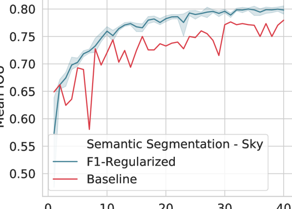
Results. Figure 3 Column 3 shows our results averaged over the thresholds . We can see that our models uniformly outperforms the baseline with a mean IOU (over baseline). Furthermore, observe that our Alg. 3 is much more stable than the baseline throughout the training process even in nonconvex settings while requiring the fewest projection steps.
Takeaway #2. Performance boosts from the F1-regularizer carries over from the simple convex classification task to the pixel-wise classification task with a deep neural network.
Experiment 3) Improving Semantic Segmentation with Nondecomposable Regularizers
Dataset. We are now ready to consider semantic segmentation with multiple classes in each image. Our dataset consists of images that belong to any of the “stuff” classes in the MSCOCO “Stuff” dataset Caesar et al. (2018). We downsampled the training images to size to reduce training time.
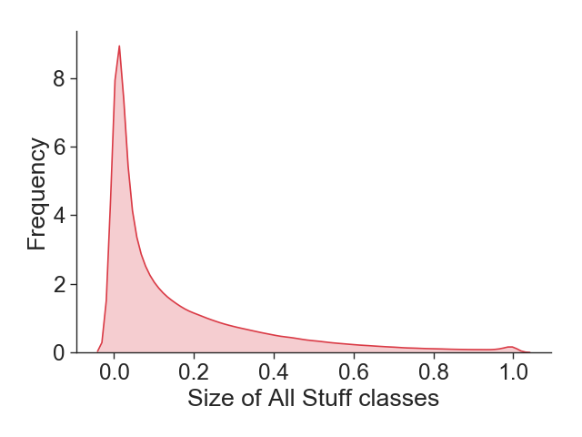
How to obtain size ? The volume of stuff denoted by is measured by the number of pixels that belong to . We observed that is close to for most (see appendix). So, we picked a threshold of to obtain a binary for each class . Then, we use the majority vote provided by all classes present in an image to obtain for individual images – corresponding to “big/small”. That is, if the majority of the classes present inside the image are “big” (as determined by the threshold ), then we assigned the image to be “big” and vice-versa.
Model and Training. We use DeepLabV3+ model proposed in Chen et al. (2018) for training. DeepLabV3+ is a popular model for semantic segmentation (needs no CRF post-processing) and can be trained end-to-end. We used a minibatch size of for baseline and for our regularized models.
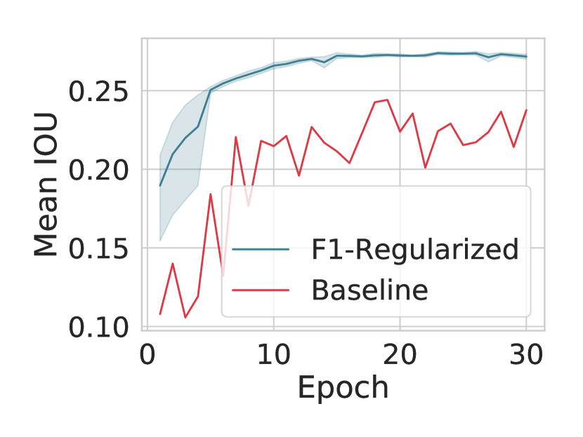
Results. Figure 5 Column 1 shows the quantitative results of our experiment averaged over the thresholds . Columns 2-4 shows some of our qualitative results. See appendix for quantitative results on MSCOCO stuff segmentation benchmark. Our mean IOU improves upon the state of the art reported in Chen et al. (2018) by on MSCOCO 164K while being stable.
Takeaway #3. On the MS COCO 164K Stuff dataset, we achieve state of the art results with Mean IOU (vs. current state of the art mean IOU in Chen et al. (2018)).
5 Conclusions
While nondecomposable data-dependent regularizers are variously beneficial and needed in a number of applications, their benefits cannot often be leveraged in large scale settings due to computational challenges. Further, the literature provides little guidance on mechanisms to utilize such regularizers within the deep neural network architectures that are commonly used in the community. In this paper, we showed how various nondecomposable regularizers may indeed permit highly efficient optimization schemes that can also directly benefit from the optimization routines implemented in mature software libraries used in vision and machine learning. We provide a technical analysis of the algorithm and show that the procedure yields state of the art performance for a semantic segmentation task, with only minimal changes in the optimization routine.
References
- Allen-Zhu (2018) Zeyuan Allen-Zhu. Natasha 2: Faster non-convex optimization than sgd. In Advances in neural information processing systems, pages 2675–2686, 2018.
- Badrinarayanan et al. (2017) Vijay Badrinarayanan, Alex Kendall, and Roberto Cipolla. Segnet: A deep convolutional encoder-decoder architecture for image segmentation. IEEE transactions on pattern analysis and machine intelligence, 39(12):2481–2495, 2017.
- Baydin et al. (2018) Atilim Gunes Baydin, Barak A Pearlmutter, Alexey Andreyevich Radul, and Jeffrey Mark Siskind. Automatic differentiation in machine learning: a survey. Journal of machine learning research, 2018.
- Caesar et al. (2018) Holger Caesar, Jasper Uijlings, and Vittorio Ferrari. Coco-stuff: Thing and stuff classes in context. In Computer vision and pattern recognition (CVPR), 2018.
- Caravenna and Daneri (2010) Laura Caravenna and Sara Daneri. The disintegration of the lebesgue measure on the faces of a convex function. Journal of Functional Analysis, 2010.
- (6) Jie Chen and Ronny Luss. Stochastic gradient descent with biased but consistent gradient estimators. arXiv:1807.11880.
- Chen et al. (2018) Liang-Chieh Chen, Yukun Zhu, George Papandreou, Florian Schroff, and Hartwig Adam. Encoder-decoder with atrous separable convolution for semantic image segmentation. In Proceedings of the European Conference on Computer Vision (ECCV), pages 801–818, 2018.
- Chenxi and Fine (2012) Li Chenxi and Jason Fine. Smoothed nonparametric estimation for current status competing risks data. Biometrika, 2012.
- Cheung et al. (2014) Brian Cheung, Jesse A Livezey, Arjun K Bansal, and Bruno A Olshausen. Discovering hidden factors of variation in deep networks. arXiv preprint arXiv:1412.6583, 2014.
- Corduneanu and Jaakkola (2006) Adrian Corduneanu and Tommi Jaakkola. Data dependent regularization. Semi-Supervised Learning, pages 163–182, 2006.
- Cotter et al. (2018) Andrew Cotter, Heinrich Jiang, Serena Wang, Taman Narayan, Maya Gupta, Seungil You, and Karthik Sridharan. Optimization with non-differentiable constraints with applications to fairness, recall, churn, and other goals. arXiv preprint arXiv:1809.04198, 2018.
- Cotter et al. (2019) Andrew Cotter, Maya Gupta, Heinrich Jiang, Erez Louidor, James Muller, Tamann Narayan, Serena Wang, and Tao Zhu. Shape constraints for set functions. In ICML, 2019.
- Cuturi et al. (2019) Marco Cuturi, Olivier Teboul, and Jean-Philippe Vert. Differentiable sorting using optimal transport: The sinkhorn cdf and quantile operator. arXiv preprint arXiv:1905.11885, 2019.
- Daimon et al. (2018) Takashi Daimon, Akihiro Hirakawa, and Shigeyuki Matsui. An Introduction to Dose-Finding Methods in Early Phase Clinical Trials. Springer, 2018.
- Dieuleveut et al. (2017) Aymeric Dieuleveut, Alain Durmus, and Francis Bach. Bridging the gap between constant step size stochastic gradient descent and markov chains. arXiv preprint arXiv:1707.06386, 2017.
- Eban et al. (2016) Elad ET Eban, Mariano Schain, Alan Mackey, Ariel Gordon, Rif A Saurous, and Gal Elidan. Scalable learning of non-decomposable objectives. arXiv preprint arXiv:1608.04802, 2016.
- Faden et al. (1985) Arnold M Faden et al. The existence of regular conditional probabilities: necessary and sufficient conditions. The Annals of Probability, 1985.
- Groeneboom and Jongbloed (2014) Piet Groeneboom and Geurt Jongbloed. Nonparametric Estimation under Shape Constraints: Estimators, Algorithms and Asymptotics. Cambridge Series in Statistical and Probabilistic Mathematics. Cambridge University Press, 2014. doi: 10.1017/CBO9781139020893.
- Kar et al. (2014) Purushottam Kar, Harikrishna Narasimhan, and Prateek Jain. Online and stochastic gradient methods for non-decomposable loss functions. In Advances in Neural Information Processing Systems, 2014.
- Lezama et al. (2018) José Lezama, Qiang Qiu, Pablo Musé, and Guillermo Sapiro. Olé: Orthogonal low-rank embedding-a plug and play geometric loss for deep learning. In Proceedings of the IEEE Conference on Computer Vision and Pattern Recognition, 2018.
- Limentani et al. (2005) Giselle B Limentani, Moira C Ringo, Feng Ye, Mandy L Bergquist, and Ellen O McSorley. Beyond the t-test: statistical equivalence testing, 2005.
- (22) Zachary C Lipton, Charles Elkan, and Balakrishnan Naryanaswamy. Optimal thresholding of classifiers to maximize f1 measure. In Joint European Conference on Machine Learning and Knowledge Discovery in Databases. Springer.
- (23) Xiaolong Liu, Zhidong Deng, and Yuhan Yang. Recent progress in semantic image segmentation. Artificial Intelligence Review.
- Long et al. (2015) Jonathan Long, Evan Shelhamer, and Trevor Darrell. Fully convolutional networks for semantic segmentation. In IEEE conference on computer vision and pattern recognition, 2015.
- Mahdavi et al. (2012) Mehrdad Mahdavi, Tianbao Yang, Rong Jin, Shenghuo Zhu, and Jinfeng Yi. Stochastic gradient descent with only one projection. In Advances in Neural Information Processing Systems, 2012.
- Mou et al. (2018) Wenlong Mou, Yuchen Zhou, Jun Gao, and Liwei Wang. Dropout training, data-dependent regularization, and generalization bounds. In ICML, 2018.
- Narasimhan et al. (2014) Harikrishna Narasimhan, Rohit Vaish, and Shivani Agarwal. On the statistical consistency of plug-in classifiers for non-decomposable performance measures. In Advances in Neural Information Processing Systems, 2014.
- Rippel et al. (2015) Oren Rippel, Manohar Paluri, Piotr Dollar, and Lubomir Bourdev. Metric learning with adaptive density discrimination. arXiv preprint arXiv:1511.05939, 2015.
- Sanyal et al. (2018) Amartya Sanyal, Pawan Kumar, Purushottam Kar, Sanjay Chawla, and Fabrizio Sebastiani. Optimizing non-decomposable measures with deep networks. Machine Learning, 2018.
- Shah (2017) Meet P Shah. Semantic segmentation architectures implemented in pytorch. https://github.com/meetshah1995/pytorch-semseg, 2017.
- Tropp (2015) Joel A. Tropp. An introduction to matrix concentration inequalities, 2015. URL http://arxiv.org/abs/1501.01571.
- Wager et al. (2013) Stefan Wager, Sida Wang, and Percy S Liang. Dropout training as adaptive regularization. In Advances in neural information processing systems, 2013.
- Yin and Yu (2018) Junming Yin and Yaoliang Yu. Convex-constrained sparse additive modeling and its extensions. CoRR, 2018.
- Zhang et al. (2018) Xiaoxuan Zhang, Mingrui Liu, Xun Zhou, and Tianbao Yang. Faster online learning of optimal threshold for consistent f-measure optimization. In Advances in Neural Information Processing Systems, pages 3889–3899, 2018.
- Zhao et al. (2019) Zhong-Qiu Zhao, Peng Zheng, Shou-tao Xu, and Xindong Wu. Object detection with deep learning: A review. IEEE transactions on neural networks and learning systems, 2019.
- Zhou et al. (2016) Bolei Zhou, Aditya Khosla, Agata Lapedriza, Aude Oliva, and Antonio Torralba. Learning deep features for discriminative localization. In Proceedings of the IEEE conference on computer vision and pattern recognition, 2016.
- Zhou et al. (2017) Hao Henry Zhou, Yilin Zhang, Vamsi K Ithapu, Sterling C Johnson, Vikas Singh, et al. When can multi-site datasets be pooled for regression? hypothesis tests, -consistency and neuroscience applications. In ICML, 2017.
- Zhu et al. (2018) Wei Zhu, Qiang Qiu, Jiaji Huang, Robert Calderbank, Guillermo Sapiro, and Ingrid Daubechies. Ldmnet: Low dimensional manifold regularized neural networks. In The IEEE Conference on Computer Vision and Pattern Recognition (CVPR), 2018.
Appendix
6 Extending our results to other Metrics
Point Metrics. To see how to extend our results to say R@Pα metric, we simply note that both recall and precision can be represented as rate constraints, as discussed in Cotter et al. (2018). This means that we can simply reparameterize these terms as shown in the main paper, and does not require a linear fractional transformation that we need to use for type metrics.
Integral Metrics. To extend to AUCROC type metrics that are defined as integrals over the point metrics, we can use Nystrom Approximation. That is, we first choose a sufficiently fine grid (at many ’s), and then reparameterize the R@P at each point () in the grid. Hence, the convergence guarantee in Theorem 1 apply in both of these settings.
7 Missing details from Section 3 in the Main Paper
7.1 Generalizing to finite
First we discuss on how to generalize our formulation when finite . For our purposes, we may assume from now on that is linear, parameterized by (without of loss generality) since we can use the reparameterization shown in the main paper. Furthermore as in section 3 of the main paper, we may ignore the ERM term. When , there are several ways to generalize the metric, see Section 6 Lipton et al. . Essentially, the score may simply be between each pair of classes in the training data. This will lead to constraints of the form,
| (8) |
where represents the th column of (th size predictor) and represents the margin of example with respect to the size predictor given by . Following the reparameterization technique in Section 3 in the main paper, we simply dualize the complicating constraints shown in (8) by introducing dual variables .
Remark 8
Observe that Algorithm 1 remains unchanged after the addition of dual variables. Naturally, the convergence of Algorithm 1 depends on the number . Without further assumptions on the data (such as separability) it is currently not possible to obtain convergence rate with no dependence on , see Allen-Zhu (2018).
7.2 Proof of Lemma 1 in the main paper
Recall that the Euclidean projection amounts to solving the following quadratic program:
| (9) |
Lemma 9
There exists an algorithm to solve (9) that requires only sorting and thresholding operations.
Proof WLOG, we can assume that since when given any , we may rearrange the coordinates. We may also assume that for any , by picking an arbitrary order for coordinates with the same value. Denoting the lagrange multipliers for the constraints in in (9), the feasibility conditions for (9) can be written as,
| (10) |
The first order necessary conditions can be written as,
| (11) |
Finally, the complementarity slackness condition between the primal and dual variables can be written as,
| (12) |
From (11), we have that which implies that and . From (12), either or , and . Let be the (active) set of indices at the optimal solution. Given , we can easily find by solving the following 1D quadratic problem
| (13) |
So, it is now
clear that in order to satisfy the feasibility conditions (10),
we simply choose the first coordinates of to be the index set , and
set
to be the average of where .
7.3 Algorithm 1: Implementation and Computational Complexity
Now, we will provide the full details of Algorithm 1 in the main paper here in Algorithm 3. We now state the definition of our lagrangian (for convenience),
| (14) |
Computational Trade-off. We can now clearly see the trade-off between doing projections done at every iteration (referred to as “Full” projections) and our reparameterized dual ascent procedure that requires only one projection for one epoch. As we can see from Algorithm 4 here, the computational burden of projection is due to sorting that is required. if , then doing full projections is attractive, whereas for large batch training, say , our algorithm 3 – reparameterized dual ascent is a much more efficient strategy.
Counting Projections. Keeping all other parameters the same, the computational complexity of full projections method will be whereas it is only in the worst case for every epoch. This means that, if we are closer to a local minima (small ), then using full projections is cheaper since it is independent of the dataset size . However, as mentioned in the main paper in the worst case to obtain an approximate (gradient norm) solution of the lagrangian (inner loop). Hence, Algorithm 1 is preferable if we are far from the optimal solution (random initialization of weights) and use full projections when using a pretrained model to fine tune the weights.
7.4 Constants in the Proof of Theorem 2
We recall the theorem statement.
Theorem 10
Assume that , and in the ERM term in Prob. (1). Then, Alg. 3 converges to a approximate (local) solution of Prob. (14) in iterations.
Proof We will use Theorem 1 in Mahdavi et al. (2012) with and .
With a slight abuse of notation we will use the matrix to represent the feasible set since there is no confusion here. Hence the feasible set can be written as,
| (15) |
with
| (16) |
Since linear functions are lipschitz, we have the required constants for Theorem 1 in Mahdavi et al. (2012) for our choice of to bne constants as and .
7.5 One Pass Algorithm to compute in Algorithm 2 in the Main Paper
We will use the following notation to slice coordinates: for a vector , selects the subspace parameterized by coordinates from to (and including) . We will now provide the sequential algorithm to implement Algorithm 2 in the main paper in here in Algorithm 4. Observe that the online nature of the algorithm suggests that we may simply compute using sampling/sketching procedures, that is, pick a sample of of size , sort it and compute the threshold. For certain distributions of , can be approximated using samples – independent of the training dataset size Tropp (2015).
7.6 Approximating for Backpropagation
Recall that our primary goal is to solve our optimization problem (14) using backpropagation based methods. In the previous sections, we argued that SGD can be used to solve (14). In particular, we showed in Theorem 10 that Algorithm 3 requires fewer projections compared to the classical PGD algorithm. It turns out that the simplicity of the projection operator can be exploited to avoid the double for loops in Algorithm 3, thus enabling backpropagation based training algorithms to be effectively deployed. We rely on the following simple, yet crucial observation,
Observation 2
Given in Algorithm 4, can be computed using the rectified linear unit (relu) function as follows,
| (17) |
where the and are applied elementwise.
To verify equation (17), note that by definition of , the first coordinates are no larger than and the remaining coordinates are strictly smaller than . Now we will show how to compute using differentiable techniques. Our approach involves four steps:
-
1.
(Differentiable Sort.) The first key step is to use recently developed algorithms to produce an approximate sorting of using Optimal Transport theory, see Cuturi et al. (2019). In particular, we first sort the input to using the so-called Sinkhorn iteration. From now on, we assume that is sorted in decreasing order of magnitues as required by Algorithm 4 in Step 4.
-
2.
(Vector of top averages.) Secondly, we compute the vector of top averages of .
-
3.
(Computing in Algorithm 4.) Define to be the vector shifted by one coordinate, that is, the th coordinate of is given by the th coordinate of with a in the last coordinate. Note that by the monotonicity of , we have that, . Hence, we have that where is defined as,
(18) In words, the inner operation compares the top averages with the th coordinate and sets the bottom coordinates to zero whereas the outer operation sets the top to one.
-
4.
(Recovering .) Finally, we can easily compute as,
(19) where corresponds to the vector of all ones and represents the diagonal matrix with entries given by the vector .
Note that computing just involves a single matrix-vector product. That is, given , we can compute by applying the lower triangular matrix with all entries in the th row given by to . Hence, all the four steps mentioned above can be unrolled into a “forward pass”, we can compute the gradient with respect to the trainable parameters of our network using the adjoint method or backpropagation, see Baydin et al. (2018).
8 Bimodal MNIST using Unimodal MNIST
Here, we show the histograms of the size of digits in our MNIST created using MNIST as discussed in Section 4.1 in the main paper in Figure 6. Observe that while the distributions of the size of each digit look approximately similar, the modes of certain digits in MNIST are closer (like ) whereas the other digits are more separated () – this slight variation is captured nicely by our metric regularized models, thereby preserving the accuracy to a larger extent than the baseline.
9 Why Choose the Category “Sky” in MSCOCO
Essentially, we observed that images corresponding to the class sky has the most amount of variance with respect to size as shown in Figure 7. In Figure 7, the histogram of the Sky class is shown on the left with a typical class from MS-COCO dataset shown on the right. Notice that the tail of the Sky class is significantly fatter than that of a typical class. Even though the Sky class is bimodal, our experimental results in the main paper show that nondecomposable regularizers can provide significant benefits for classes with fat tails.
10 Additional Results on MS-COCO Full Dataset
We provide the quantitative comparison of baseline and our algorithm mentioned in the main paper.
Now we provide some more qualitative results of our Algorithm 1 on the full MS-COCO dataset which consists of images to substantiate our claim that both small/large sized objects are segmented equally well when models are regularized with data dependent nondecomposable regularizers.


