First order phase transitions in the square lattice “easy-plane” J-Q model
Abstract
We study the quantum phase transition between the superfluid and valence bond solid in “easy-plane” J-Q models on the square lattice. The Hamiltonian we study is a linear combination of two model Hamiltonians: (1) an SU(2) symmetric model, which is the well known J-Q model that does not show any direct signs of a discontinuous transition on the largest lattices and is presumed continuous, and (2) an easy plane version of the J-Q model, which shows clear evidence for a first order transition even on rather small lattices of size . A parameter ( being the easy-plane model and being the SU(2) symmetric J-Q model) allows us to smoothly interpolate between these two limiting models. We use stochastic series expansion (SSE) quantum Monte Carlo (QMC) to investigate the nature of this transition as is varied - here we present studies for and . While we find that the first order transition weakens as is increased from 0 to 1, we find no evidence that the transition becomes continuous until the SU(2) symmetric point, . We thus conclude that the square lattice superfluid-VBS transition in the two-component easy-plane model is generically first order.
I Introduction
The quantum transition from Néel or superfluid to a valence bond solid (VBS) has been proposed to be described by the deconfined criticality scenario.Senthil et al. (2004a, b) In this scenario it is generically possible to have a direct continuous Néel-VBS transition. A number of field theoretic formulations that describe this putative critical point at long distances have been put forward and interesting connections between different representations have been conjectured via duality arguments. Senthil and Fisher (2006); Tanaka and Hu (2005); Wang et al. (2017) Establishing these fascinating connections non-perturbatively by lattice simulations is an exciting field of current research. In the original study two kinds of symmetries were highlighted for their possibility as platforms for deconfined criticality, an SU(2) symmetric system and a U(1)Z2 symmetric system. Physically, the SU(2) field theory could be a description for a rotationally symmetric anti-ferromagnet and its transition to a valence bond solid. The U(1)Z2 system can be thought of as a model for the same Néel-VBS transition in magnet with easy-plane anisotropy or alternatively as a model for a superfluid to Mott transition. 111We will use the terms magnetic and superfluid interchangeably throughout this manuscript
In the years since the original proposal, it has been demonstrated that the Néel-VBS transition and many of its variants can be studied in sign problem free quantum spin Hamiltonian models on large lattices.Kaul et al. (2013) Through extensive numerical simulations in the SU(2) symmetric models many aspects of the proposal have been borne out and no direct evidence for a first order transition has been observed. Sandvik (2007); Melko and Kaul (2008); Lou et al. (2009); Sandvik (2010a); Banerjee et al. (2010); Pujari et al. (2013); Harada et al. (2013); Pujari et al. (2015); Shao et al. (2016, 2017); Li et al. (2019) Numerical studies of classical statistical mechanics models of tightly packed loops and dimer models in three dimensions that have been argued to realize the same universal physics as the SU(2) Néel-VBS transition are also consistent with the deconfined criticality scenario. Nahum et al. (2015); Powell and Chalker (2008, 2009); Charrier et al. (2008); Chen et al. (2009); Sreejith and Powell (2014); Alet et al. (2006) Despite this large body of evidence for the deconfined criticality scenario, numerical studies have observed scaling violations whose origin is currently unclear.Kaul (2011); Nahum et al. (2015); Jiang et al. (2008); Kuklov et al. (2006); Shao et al. (2016)
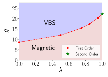
In contrast in the easy-plane case where SU(2) is broken to U(1) a number of numerical studies have concluded that the transition is first order.Sandvik et al. (2002); Kragset et al. (2006); Kuklov et al. (2006); Sen et al. (2007); D’Emidio and Kaul (2016, 2017) Recently however it has been claimed that a continuous transition has been found in a square lattice model with somewhat weaker easy-plane anisotropy,Qin et al. (2017); Ma et al. (2018) suggesting that perhaps a large easy-plane anisotropy could result in a first order transition, and the first order and second order regime are separated by a multicritical point.222We note for completeness that a model of hard core bosons at 1/3 filling on the Kagome lattice has been argued to be described by a similar field theory and host a putative easy-plane deconfined critical point.Zhang et al. (2018) Although it was originally determined to have a first order transition,Isakov et al. (2006) it has been claimed in recent work to host a continuous transition.Zhang et al. (2018) Motivated by this study, we address the issue of how the easy-plane transition is connected to the symmetric one, by studying a model that interpolates between these two limiting cases on the square lattice. For the symmetric model we use the popular J-Q model which shows no direct evidence for first order behavior even on the largest studied lattice sizes. For the easy plane case we use an easy-plane J-Q that was shown to have a first order transition already visible on . The interpolating model introduced in detail below is slightly different from the one studied in Ref. Qin et al., 2017; Ma et al., 2018 where the easy-plane anisotropy was introduced only in the J-term; both models are believed to have the same universal features however. In this work we present studies on larger lattices and a more thorough analysis. Contrary to the previous study, we find no evidence for new continuous easy-plane criticality. Instead we find a first order transition for that weakens as is increased and we approach the symmetric point () at which all our direct signals of a first order transition vanish and the transition is presumed continuous. This is the primary result of our paper and is summarized in Fig. 1. Although no numerical study can rule out that the transition becomes continuous for a very small but finite window close to (with finite easy-plane anisotropy), we find this rather unlikely given our results below. We thus conclude that the easy-plane Néel-VBS transition is generically first order on the square lattice.
II The Model
The Hamiltonian studied here is an system on an square lattice,
| (1) |
and is a linear combination of two parts, is the SU(2) symmetric part and is the easy plane part that explicitly breaks the SU(2) symmetry. is an anisotropy parameter that allows us to smoothly interpolate between the easy plane limit () and the SU(2) symmetric limit (). We define the singlet projection operator on a bond between two sites and as,
| (2) |
, are standard spin- operators where are Pauli matrices.
Then , which is the well known J-Q model, Sandvik (2007) can be written as,
| (3) |
The second term in the above equation is a sum over all elementary plaquettes . has full SU(2) symmetry inherited from . Similarly if we define
| (4) |
the easy plane Hamiltonian, can be written as,D’Emidio and Kaul (2016)
| (5) |
has a symmetry of U(1) Z2, which corresponds to U(1) rotations about the -axis and the Z2 operation of a rotation about the -axis.
We study the quantum phase transition from the magnetic phase to the valence-bond solid (VBS) phase as is varied for a fixed . While in the easy plane limit, i.e. , this transition has been found to be first order, D’Emidio and Kaul (2016) it has been argued to be to continuous in the SU(2) symmetric limit, . Sandvik (2007); Melko and Kaul (2008); Sandvik (2010a); Harada et al. (2013) In this work we interpolate between the two limiting models with the aim of elucidating the evolution of the nature of the quantum transition and in particular to investigate whether the transition is continuous for any .
III Numerical Simulations
The numerical results presented below have been obtained using the stochastic series expansion (SSE) quantum Monte Carlo method. Sandvik (2010b) We use the directed loop algorithm Syljuåsen and Sandvik (2002) to carry out global loop updates on our Monte Carlo configurations (see Appendix A.1).
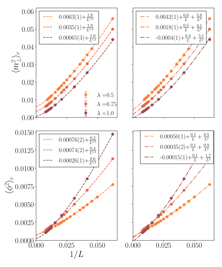
| per degree of freedom | ||||
| Power law | Polynomial | Power law | Polynomial | |
|---|---|---|---|---|
| 0.5 | 0.43 | 0.4 | 0.17 | 0.23 |
| 0.75 | 1.3 | 1.0 | 0.42 | 0.89 |
| 1.0 | 0.53 | 1.8 | 1.25 | 0.69 |
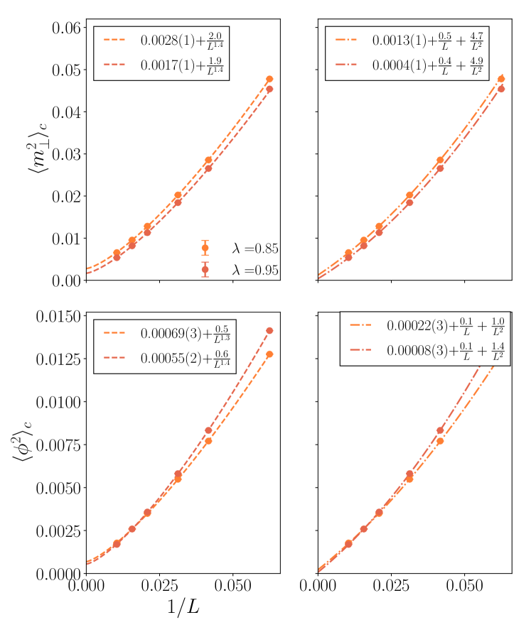
| per degree of freedom | ||||
| Power law | Polynomial | Power law | Polynomial | |
|---|---|---|---|---|
| 0.85 | 1.96 | 0.79 | 0.71 | 1.23 |
| 0.95 | 0.62 | 2.87 | 2.4 | 1.35 |
Fig. 1 shows a phase diagram obtained from numerical simulations as a function of the coupling and the anisotropy parameter . For a given , on increasing we find a quantum phase transition from the magnetic to the VBS phase. Here, we work in units where and at an inverse temperature for an lattice. All data presented has been tested to be in the limit as demonstrated in Appendix A.4.
III.1 Measurements
When , the presence of a small amount of anisotropy makes the spins preferentially align in the plane. Therefore as we vary in our simulations, we look for a phase transition between the order (superfluid) and VBS phases. We define the following quantities to detect magnetic order,
| (6) |
| (7) |
The square of the superfluid order parameter is . The quantity is measured during the loop update by keeping track of the distance between the head and the tail of the loop when they are at the same time slice. Dorneich and Troyer (2001) We also define a Néel order parameter square as . When , , and are equivalent and therefore and are equal upto a normalization.
VBS order is one where each spin forms a singlet with its neighbour and the pattern of singlets forms columnar order. We construct the VBS order parameter square from the following quantity,
| (8) |
Here is a plaquette operator which equals the sum of all the operators in the Hamiltonian acting on the plaquette at as described in Appendix A.
The spin stiffness is defined as,
| (9) |
Here E() is the energy of the system with a twist of in the boundary condition in either the or the direction. In the QMC, this quantity is related to the winding number of loops in the direction that the twist has been added, Sandvik (1997)
| (10) |
where is the inverse temperature. goes to a finite value in the magnetically ordered phase but goes to 0 otherwise. The quantity is expected to show a crossing for different values of at the coupling at which magnetic order is destroyed.
In order to detect the ordered phase we make use of ratios defined as,
| (11) |
Here ; and are the ordering momentum and momentum closest to the ordering momentum respectively. In the ordered phase goes to 1 and in the disordered phase it goes to 0 on increasing system size, therefore they are expected to cross for different system sizes at the critical point.
III.2 Numerical Results
In this work, we focus on four values of the anisotropy parameter, , , and . We have included a comparison with the symmetric case when appropriate.
III.2.1 Crossing Analysis
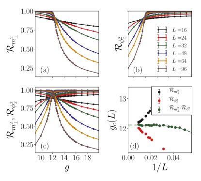
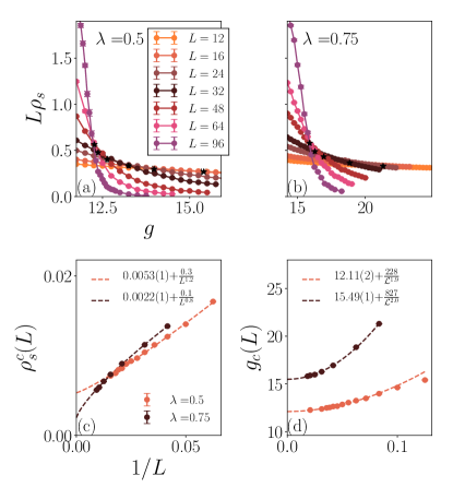
Fig. 2 (a) and (b) show ratios and (defined above) crossing for different for . This indicates a transition from the magnetic to VBS phase. Fig. 2(c) shows crossing of these ratios for the same . As shown in 2(d), the crossing analysis from 2(c) yields the transition point to be at , which is close to the value at which the couplings at the crossing points, , converge. This extrapolation has been done only using small system sizes, . We notice that smaller system sizes can be seen to smoothly converge to , bigger system sizes start deviating from this trend. This is because of the double peaked structure that starts to develop in the order parameter estimators, making it difficult to reliably extrapolate using bigger lattices. Fig. 6 shows crossings of the quantity for both and , which also indicates transition out of the magnetic phase.
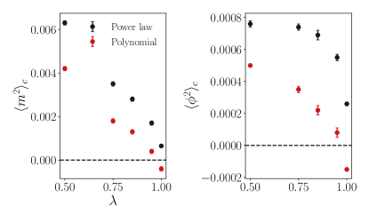
To investigate the nature of the transition, we study the extrapolation of observables with system size at the critical point. For a continuous transition, all the observables described above (, , ), should go to zero at the critical point as . Figs 3 and 4 shows values of and at the crossing points of and at extrapolated to the infinite system size limit using two different fitting forms (as described in the caption). The extrapolated values of and are clearly finite for , and . Small positive extrapolated values of these quantities using both the fit forms can also be seen for . Fig. 5 shows how the order parameter values at the transition point get progressively smaller on increasing , indicating a weakening of the first order nature. They tend to approach zero as . Therefore we can argue that the first order transition continuously evolves on varying to a second order transition at .
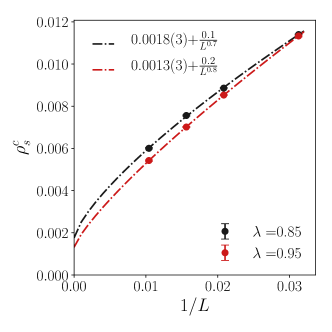
The stiffness extracted from crossings of for and in Fig 6(a),(b) is plotted as a function of in 6(c). clearly extrapolates to a finite value for for both and . Fig. 10 shows the same analysis for and . This points to a first order transition for and . For , on the other hand it is apparent from our data that is hard to argue for a finite order parameter for and from the data we have. A more thorough analysis of the is available in Ref. Shao et al., 2016. We note that these extrapolations become hard to do on very large system sizes because of ergodicity issues that we discuss below and that we argue arise fundamentally at first order transitions.
III.2.2 Histograms
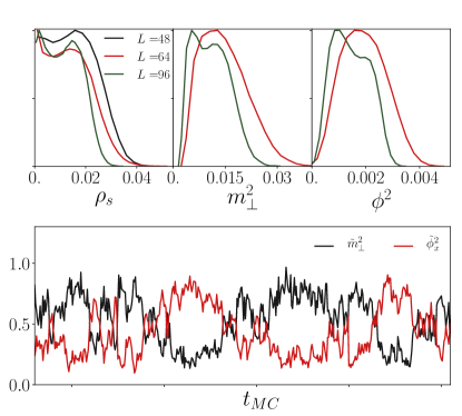
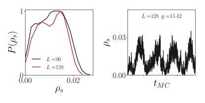
To further elucidate the nature of the transition we carefully study the histograms of observables near the critical point. Fig. 7 shows the probability distributions of the QMC estimators for , and at the transition for . There are clearly two peaks in the histograms of for , one at 0 and the other at a finite value. This double peak feature is clearly noticeable in and only for . The double peak gets more pronounced with system size which indicates that the first order behavior survives in the thermodynamic limit. The time series data shows switching between the two orders: one order parameter is finite when the other goes to 0, thus one order is present when the other is not. This is characteristic of a first order transition. This system exhibits clear first order behavior only for , therefore we conclude that this transition is a weak first order transition. The first order nature of the transition is even weaker for , the double peak in the histograms of stiffness appears for as shown in Fig. 8. We find no evidence of double peaked histograms for and for the largest system sizes studied here. However, as explained before, we do find other evidence of first order behaviour in these two cases. There is also no evidence of double peaked histograms for for the largest system size we have studied. This is consistent with the numerical findings in the past. Sandvik (2007); Melko and Kaul (2008); Sandvik (2010a); Harada et al. (2013) Therefore we conclude that the transition is first order for and . The first order behaviour gets progressively weaker as gets closer to 1, eventually disappearing at .
IV Conclusions
We studied an interpolation of two previously known and well studied models, the J-Q model Sandvik (2007) which hosts a continuous Néel-VBS transition and the easy-plane J-Q model D’Emidio and Kaul (2016) which hosts a first order superfluid-VBS transition. By studying the phase transition as a function of the parameter that interpolates between the two limits, we found the phase diagram shown in Fig. 1. Our main conclusion is that whenever the easy-plane anisotropy is present the transition is first order. All signs of discontinuity vanish only at the symmetric point . This indicates that the easy-plane anisotropy is a relevant perturabation at the SU(2) symmetric deconfined critical point and results in a runaway flow to a first order transition.
We acknowledge helpful discussions with A. Sandvik. Partial financial support was received through NSF DMR-1611161 and Keith B Macadam Graduate Excellence Fellowship. Computing resources were obtained through NSF’s XSEDE award TG-DMR-140061 and the DLX computer at the University of Kentucky.
Appendix A Details of Numerical Simulations and Checks
A.1 Lattice Hamiltonian
The Hamiltonian defined by Eq. 1 is sign problem free on a bipartite lattice 333The following unitary transformation: and , on one of the sublattices of the bipartition, yields all negative off-diagonal elements for the Heisenberg exchange which is the sign problem free condition and therefore we use the SSE QMC algorithm with directed loop updates to simulate it. The easy plane limit of this model () has no diagonal terms. Hence, to make the model easier to simulate in this limit, we add a constant to the Hamiltonian to generate diagonal matrix elements.D’Emidio and Kaul (2016) The easy plane part of the model defined in Eq. 5 then becomes:
| (12) |
To make the loop update more convenient we treat all bonds as plaquettes by multiplying an identity to the adjacent bond, for e.g. the operator in Eq. 2 gets replaced in the following way:
| (13) |
Here is an identity operator, the sum in this equation is over all four site plaquettes such that is adjacent and parallel to . is number of plaquettes each bond is a part of, which is 2 in the square lattice case. After making these substitutions the full Hamiltonian described by Eq. 1 becomes:
| (14) |
| 0.5 | 0.5 | -0.99366(6) | -0.99371 | 0.2737(1) | 0.2738 |
| 0.5 | 1.0 | -0.96744(6) | -0.96746 | 0.2375(1) | 0.2374 |
| 0.75 | 10.0 | -0.80616(6) | -0.80608 | 0.12102(7) | 0.12090 |
| 0.75 | 18.0 | -0.76614(6) | -0.76613 | 0.11319(7) | 0.11324 |
| 0.5 | 0.5 | 0.43721(6) | 0.43725 | 0.04416(2) | 0.04414 |
| 0.5 | 1.0 | 0.39560(5) | 0.39558 | 0.05884(3) | 0.05887 |
| 0.5 | 15.0 | 0.26562(3) | 0.26560 | 0.04643(2) | 0.04642 |
| 0.75 | 10.0 | 0.27187(2) | 0.27186 | 0.07704(3) | 0.07703 |
| 0.75 | 18.0 | 0.26548(2) | 0.26546 | 0.07317(2) | 0.7318 |
A.2 Plaquette Operator
The plaquette operator, in Eq. 8 is the sum of all operators in the Hamiltonian acting on the plaquette at . Let be the position vector of the lower left site of the plaquette
| (15) |
A.3 QMC vs ED
Tables LABEL:tab:obs and LABEL:tab:corr show comparison of the groundstate energy per unit site (), spin stiffness () and square of the order parameters, and , got from QMC and from exact diagonalization for and on lattices. , and are as defined in Sec. III.1.
A.4 Convergence to
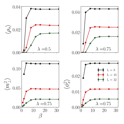
Fig. 9 shows the behaviour of the observables we have measured for square lattices as a function of inverse temperature . The measurements have been done close to the critical points ( for and for ). These quantities can be seen to saturate to the value on increasing the value of . The at which this saturation occurs depends on the system size . As we increase the system size these values saturate to the value at faster, therefore we pick for our simulations.
References
- Senthil et al. (2004a) T. Senthil, A. Vishwanath, L. Balents, S. Sachdev, and M. P. A. Fisher, Science 303, 1490 (2004a), URL http://www.sciencemag.org/content/303/5663/1490.abstract.
- Senthil et al. (2004b) T. Senthil, L. Balents, S. Sachdev, A. Vishwanath, and M. P. A. Fisher, Phys. Rev. B 70, 144407 (2004b), URL https://link.aps.org/doi/10.1103/PhysRevB.70.144407.
- Senthil and Fisher (2006) T. Senthil and M. P. A. Fisher, Phys. Rev. B 74, 064405 (2006), URL https://link.aps.org/doi/10.1103/PhysRevB.74.064405.
- Tanaka and Hu (2005) A. Tanaka and X. Hu, Phys. Rev. Lett. 95, 036402 (2005), URL https://link.aps.org/doi/10.1103/PhysRevLett.95.036402.
- Wang et al. (2017) C. Wang, A. Nahum, M. A. Metlitski, C. Xu, and T. Senthil, Phys. Rev. X 7, 031051 (2017), URL https://link.aps.org/doi/10.1103/PhysRevX.7.031051.
- Kaul et al. (2013) R. K. Kaul, R. G. Melko, and A. W. Sandvik, Annu. Rev. Cond. Matt. Phys 4, 179 (2013), URL http://www.annualreviews.org/doi/abs/10.1146/annurev-conmatphys-030212-184215.
- Sandvik (2007) A. W. Sandvik, Phys. Rev. Lett. 98, 227202 (2007), URL http://link.aps.org/doi/10.1103/PhysRevLett.98.227202.
- Melko and Kaul (2008) R. G. Melko and R. K. Kaul, Phys. Rev. Lett. 100, 017203 (2008), URL https://link.aps.org/doi/10.1103/PhysRevLett.100.017203.
- Lou et al. (2009) J. Lou, A. W. Sandvik, and N. Kawashima, Phys. Rev. B 80, 180414 (2009), URL https://link.aps.org/doi/10.1103/PhysRevB.80.180414.
- Sandvik (2010a) A. W. Sandvik, Phys. Rev. Lett. 104, 177201 (2010a), URL https://link.aps.org/doi/10.1103/PhysRevLett.104.177201.
- Banerjee et al. (2010) A. Banerjee, K. Damle, and F. Alet, Phys. Rev. B 82, 155139 (2010), URL https://link.aps.org/doi/10.1103/PhysRevB.82.155139.
- Pujari et al. (2013) S. Pujari, K. Damle, and F. Alet, Phys. Rev. Lett. 111, 087203 (2013), URL https://link.aps.org/doi/10.1103/PhysRevLett.111.087203.
- Harada et al. (2013) K. Harada, T. Suzuki, T. Okubo, H. Matsuo, J. Lou, H. Watanabe, S. Todo, and N. Kawashima, Phys. Rev. B 88, 220408 (2013), URL https://link.aps.org/doi/10.1103/PhysRevB.88.220408.
- Pujari et al. (2015) S. Pujari, F. Alet, and K. Damle, Phys. Rev. B 91, 104411 (2015), URL https://link.aps.org/doi/10.1103/PhysRevB.91.104411.
- Shao et al. (2016) H. Shao, W. Guo, and A. W. Sandvik, Science 352, 213 (2016), ISSN 0036-8075, URL https://science.sciencemag.org/content/352/6282/213.
- Shao et al. (2017) H. Shao, Y. Q. Qin, S. Capponi, S. Chesi, Z. Y. Meng, and A. W. Sandvik, Phys. Rev. X 7, 041072 (2017), URL https://link.aps.org/doi/10.1103/PhysRevX.7.041072.
- Li et al. (2019) Z.-X. Li, S.-K. Jian, and H. Yao, arXiv e-prints arXiv:1904.10975 (2019), eprint 1904.10975.
- Nahum et al. (2015) A. Nahum, J. T. Chalker, P. Serna, M. Ortuño, and A. M. Somoza, Phys. Rev. X 5, 041048 (2015), URL https://link.aps.org/doi/10.1103/PhysRevX.5.041048.
- Powell and Chalker (2008) S. Powell and J. T. Chalker, Phys. Rev. Lett. 101, 155702 (2008), URL https://link.aps.org/doi/10.1103/PhysRevLett.101.155702.
- Powell and Chalker (2009) S. Powell and J. T. Chalker, Phys. Rev. B 80, 134413 (2009), URL https://link.aps.org/doi/10.1103/PhysRevB.80.134413.
- Charrier et al. (2008) D. Charrier, F. Alet, and P. Pujol, Phys. Rev. Lett. 101, 167205 (2008), URL https://link.aps.org/doi/10.1103/PhysRevLett.101.167205.
- Chen et al. (2009) G. Chen, J. Gukelberger, S. Trebst, F. Alet, and L. Balents, Phys. Rev. B 80, 045112 (2009), URL https://link.aps.org/doi/10.1103/PhysRevB.80.045112.
- Sreejith and Powell (2014) G. J. Sreejith and S. Powell, Phys. Rev. B 89, 014404 (2014), URL https://link.aps.org/doi/10.1103/PhysRevB.89.014404.
- Alet et al. (2006) F. Alet, G. Misguich, V. Pasquier, R. Moessner, and J. L. Jacobsen, Phys. Rev. Lett. 97, 030403 (2006), URL https://link.aps.org/doi/10.1103/PhysRevLett.97.030403.
- Kaul (2011) R. K. Kaul, Phys. Rev. B 84, 054407 (2011), URL https://link.aps.org/doi/10.1103/PhysRevB.84.054407.
- Jiang et al. (2008) F.-J. Jiang, M. Nyfeler, S. Chandrasekharan, and U.-J. Wiese, Journal of Statistical Mechanics: Theory and Experiment 2008, P02009 (2008), URL https://doi.org/10.1088%2F1742-5468%2F2008%2F02%2Fp02009.
- Kuklov et al. (2006) A. Kuklov, N. Prokof’ev, B. Svistunov, and M. Troyer, Annals of Physics 321, 1602 (2006), ISSN 0003-4916, july 2006 Special Issue, URL http://www.sciencedirect.com/science/article/pii/S0003491606000789.
- D’Emidio and Kaul (2016) J. D’Emidio and R. K. Kaul, Phys. Rev. B 93, 054406 (2016), URL https://link.aps.org/doi/10.1103/PhysRevB.93.054406.
- Sandvik et al. (2002) A. W. Sandvik, S. Daul, R. R. P. Singh, and D. J. Scalapino, Phys. Rev. Lett. 89, 247201 (2002), URL https://link.aps.org/doi/10.1103/PhysRevLett.89.247201.
- Kragset et al. (2006) S. Kragset, E. Smørgrav, J. Hove, F. S. Nogueira, and A. Sudbø, Phys. Rev. Lett. 97, 247201 (2006), URL https://link.aps.org/doi/10.1103/PhysRevLett.97.247201.
- Sen et al. (2007) A. Sen, K. Damle, and T. Senthil, Phys. Rev. B 76, 235107 (2007), URL https://link.aps.org/doi/10.1103/PhysRevB.76.235107.
- D’Emidio and Kaul (2017) J. D’Emidio and R. K. Kaul, Phys. Rev. Lett. 118, 187202 (2017), URL https://link.aps.org/doi/10.1103/PhysRevLett.118.187202.
- Qin et al. (2017) Y. Q. Qin, Y.-Y. He, Y.-Z. You, Z.-Y. Lu, A. Sen, A. W. Sandvik, C. Xu, and Z. Y. Meng, Phys. Rev. X 7, 031052 (2017), URL https://link.aps.org/doi/10.1103/PhysRevX.7.031052.
- Ma et al. (2018) N. Ma, G.-Y. Sun, Y.-Z. You, C. Xu, A. Vishwanath, A. W. Sandvik, and Z. Y. Meng, Phys. Rev. B 98, 174421 (2018), URL https://link.aps.org/doi/10.1103/PhysRevB.98.174421.
- Sandvik (2010b) A. W. Sandvik, AIP Conf. Proc. 1297, 135 (2010b), URL http://scitation.aip.org/content/aip/proceeding/aipcp/10.1063/1.3518900.
- Syljuåsen and Sandvik (2002) O. F. Syljuåsen and A. W. Sandvik, Phys. Rev. E 66, 046701 (2002), URL https://link.aps.org/doi/10.1103/PhysRevE.66.046701.
- Dorneich and Troyer (2001) A. Dorneich and M. Troyer, Phys. Rev. E 64, 066701 (2001), URL https://link.aps.org/doi/10.1103/PhysRevE.64.066701.
- Sandvik (1997) A. W. Sandvik, Phys. Rev. B 56, 11678 (1997), URL https://link.aps.org/doi/10.1103/PhysRevB.56.11678.
- Zhang et al. (2018) X.-F. Zhang, Y.-C. He, S. Eggert, R. Moessner, and F. Pollmann, Phys. Rev. Lett. 120, 115702 (2018), URL https://link.aps.org/doi/10.1103/PhysRevLett.120.115702.
- Isakov et al. (2006) S. V. Isakov, S. Wessel, R. G. Melko, K. Sengupta, and Y. B. Kim, Phys. Rev. Lett. 97, 147202 (2006), URL https://link.aps.org/doi/10.1103/PhysRevLett.97.147202.