Thermodynamics and reentrant phase transition
for logarithmic nonlinear charged black holes in massive gravity

Abstract

We investigate a new class of $(n+1)$-dimensional topological black hole solutions in the context of massive gravity and in the presence of logarithmic nonlinear electrodynamics. Exploring higher dimensional solutions in massive gravity coupled to nonlinear electrodynamics is motivated by holographic hypothesis as well as string theory. We first construct exact solutions of the field equations and then explore the behavior of the metric functions for different values of the model parameters. We observe that our black holes admit the multi-horizons caused by a quantum effect called anti-evaporation. Next, by calculating the conserved and thermodynamic quantities, we obtain a generalized Smarr formula. We find that the first law of black holes thermodynamics is satisfied on the black hole horizon. We study thermal stability of the obtained solutions in both canonical and grand canonical ensembles. We reveal that depending on the model parameters, our solutions exhibit a rich variety of phase structures. Finally, we explore, for the first time without extending thermodynamics phase space, the critical behavior and reentrant phase transition for black hole solutions in massive gravity theory. We realize that there is a zeroth order phase transition for a specified range of charge value and the system experiences a large/small/large reentrant phase transition due to the presence of nonlinear electrodynamics.

I INTRODUCTION

The initial version of General Relativity (GR) presented by Einstein is a theory which predicts the existence of a massless spin-$2$ particle called graviton ref1 . One of the most natural generalizations of massless GR theory is to admit the existence of the massive graviton and hence constructing a massive theory of gravity. According to the particle physics, Higgs mechanism bestows mass to carrier particles of the electroweak interaction. Strong motivation for studying the massive gravity models comes from recent developments in gravitational waves observatory. The recent observation of the the gravitational wave event GW170817 and of its electromagnetic counterpart GRB170817A, from a binary neutron star merger, confirmed that the speed of gravitational waves deviates from the speed of light by less than one part in $10^{15}$ Abbot1 . This implies that one should consider an upper bound for the mass of graviton Abbot2 . Thus the observation of the gravitational waves put severe constraints on several theories of modified gravity. Any modified gravity model predicting the speed of gravitational waves less than the speed of light must now be seriously reconsidered Ales . From holographic point of view, massive gravity could make momentum dissipative in dual systems ref8 . Giving mass to graviton state breaks the diffeomorphism invariance of stress-energy tensor of dual theory holographically which in turn cause momentum dissipation ref8 .

Historically, the first massive gravity theory was derived by Fierz and Pauli by adding the interaction terms to the linearized level of GR ref3 . Their theory suffered a discontinuity in the predictions. For instance, Van Dam, Veltman and Zakharov found a discontinuity in the Newtonian potential in massless limit, recognized as VDVZ problem ref4 . Boulware and Deser suggested a nonlinear model ref5 , while Vainshtein introduced the linearized theory as culprit for VDVZ problem ref16 . However, their theory was plagued with a ghost appeared as a 6th degree of freedom. A four-dimensional covariant nonlinear theories of massive gravity which are ghost-free in the decoupling limit to all orders was established by de Rham-Gabadadze-Tolley (dRGT) ref6 . Their theories resum explicitly all the nonlinear terms of an effective field theory of massive gravity ref6 . Actually, the absence of higher derivative terms in equations of motion does not allow the ghost to exist. This theory has been explored from different point of view and known as the only candidate for pathology-free nonlinear massive gravity so far ref13 . Although, finding exact solutions is not easy in this model due to the complexity of equations, it has always been an interesting and well motivated topic of research in theoretical physics ref11 .

Black hole solutions in the context of massive gravity have been explored from different points of view. A Schwarzschild-de Sitter-like vacuum solution of dRGT model has been found in ref7 . A nontrivial black hole solution with a negative cosmological constant has been obtained in ref8 . It has been shown that the mass of the graviton in massive theory is equivalent to the lattice in the holographic conductor model ref8 (see also ref9 ). Charged black hole solutions of massive gravity theory with negative cosmological constant have been constructed in ref10 and their thermodynamic properties and phase structure have been studied in both canonical and grand canonical ensembles. Exact three-dimensional asymptotically AdS-like solutions in massive gravity have been explored in ref12 . The authors of Ref. ref17 found the classical solutions for stars and other compact objects in massive gravity following the Vainshtein mechanism. Neutron stars in the context of this theory have been investigated in ref18 .

The importance of massive gravity does not restrict to the non-perturbative aspects of gravity or black hole solutions. In the cosmological framework, the massive gravity can be regarded as an alternative for the late time cosmic acceleration cosmicAcc . Thanks to Vainshtein mechanism, massive gravity is equivalent to GR at small scales, although in large distances (i.e. infrared regime) it amends gravity. Thus, the nature of the cosmological constant may change since it is the most universal infrared possible source ref14 . Furthermore, massive particles generate Yukawa potential $\sim{e^{-m\,r}}/{r}$ which has an exponential suppression kicking in at the length scale $\sim{1}/{m}$. If we imagine that $m\sim H$ where $H$ is Hubble scale, then the force of massive graviton would be weakened at large scales and it may offer a nice solution for acceleration problem ref15 . More researches in this regard can be found in ref19 .

When the linear Maxwell theory failed to explain the central singularity of a point charge, the striking alternative was nonlinear electrodynamics (NED). In $1930$, Born and Infeld (BI) made the first efforts to construct a NED theory ref20 . Some years later, it turned out that their theory plays a prominent role in D-brane physics. In the framework of particle physics, NED was propounded by Heisenberg and Euler ref21 . Its extension in GR was done by Plebanski ref22 . The theories of NED have arisen a lot of attention after development in the string theory ref23 . For instance, loop calculations in open superstring theory lead to a low energy effective action included BI type term ref26 . It is noteworthy to mention that at the high energy levels, due to the interactions with other physical fields, real electromagnetic field cannot obey linear law. Basically, it was argued that NEDs are the simplified phenomenological descriptions of the pointed out interactions. In addition, NED can explain the Rindler acceleration as a nonlinear electromagnetic effect ref24 . From quantum gravity viewpoint, NEDs are corrections to Maxwell field. So, a large class of regular black holes (i.e. black holes without singularity) have been studied in the literature. The pioneer effort in this direction is attributed to Bardeen ref25 .

The Lagrangian of a general theory of NED is assumed to be a function of the Maxwell invariant $\mathcal{F}=F_{\mu\nu}F^{\mu\nu}$ where $F_{\mu\nu}$ is electromagnetic tensor and not to contain any higher derivative terms of $\mathcal{F}$. In the weak field limit, these theories lead to linear Maxwell one and so their expansions in terms of $\mathcal{F}$ have the form $\mathcal{L}(\mathcal{F})=\mathcal{F}+O(\mathcal{F}^{2})$. There has been some efforts to construct BI type NED Lagrangian in literature. Two famous ones are so-called Logarithmic (LNE) and Exponential (ENE) nonlinear electrodynamics ref27 ; ref28 . LNE removes divergences in the electric field (like BI model), whereas the ENE just makes it weaker than Maxwell theory. In the present work, we are interested in considering LNE Lagrangian. It is notable to mention that logarithmic term of the field strength may come out as an exact one-loop correction to the vacuum polarization. This fact has been proved by Euler and Heisenberg when they studied electrons in a background setup by a uniform electromagnetic field ref21 .

LNE Lagrangian has been studied in various contexts. In Einstein-dilaton theory, black hole solutions have been constructed and their thermodynamic stability have been discussed ref30 . AdS-dilaton black holes in the presence of LNE have been investigated in ref31 . Lifshitz-dilaton black holes/branes coupled to LNE have been investigated in ref32 . Magnetic rotating dilaton strings and charged rotating dilaton black strings in Einstein gravity with LNE electrodynamics have been found in ref33 and ref34 , respectively. In the context of Lovelock gravity, authors of ref35 explored magnetic brane solutions in the presence of LNE. Other studies on the black hole solutions in the presence of LNE can be carried out in ref38 .

The layout of this paper is as follows. In the next section, we introduce the Lagrangian of massive gravity in the presence of cosmological constant and LNE and construct exact black hole solutions. We calculate conserved and thermodynamic quantities of the solutions in section III. Thermal stability of the solutions is checked in IV. In V, the critical behavior of ($3+1$)-dimensional black holes is examined. We devoted the last section to summary and some closing remarks.

II Action and massive gravity solutions

The ($n+1$)-dimensional action of Einstein massive gravity with a negative cosmological constant and NLE is maldacena

$$\mathcal{S}=\frac{1}{16\pi}\int d^{n+1}x\sqrt{-g}\left[\mathcal{R}-2\Lambda-8\beta^{2}\ln\left(1+\frac{\mathcal{F}}{8\beta^{2}}\right)+m^{2}\sum_{i}^{4}c_{i}\mathcal{U}_{i}(g,\Gamma)\right],$$ (1)

where $\mathcal{R}$ is the Ricci scalar, $\Lambda=-n(n-1)/2l^{2}$ with $l$ is the radius of AdS spacetime and $\mathcal{F}=F_{\mu\nu}F^{\mu\nu}$ is the Maxwell invariant and $F_{\mu\nu}=2\partial_{[\mu}A_{\nu]}$ is the electromagnetic field tensor, while $A_{\nu\text{ \ }}$ is the electromagnetic vector potential. The constant $\beta$ is the parameter of nonlinearity so that the logarithmic nonlinear electrodynamics recovers the linear Maxwell theory when $\beta\rightarrow\infty$. $m^{2}$ is the positive massive gravity parameter so that the translational invariance is recovered as $m$ approachs to zero $(m\rightarrow 0).$

In action (1), $c_{i}$’s are constants and $\mathcal{U}_{i}$’s are symmetric polynomials eigenvalues of $(n+1)\times(n+1)$ matrix $\mathcal{K}_{\nu}^{\mu}=\sqrt{g^{\mu\lambda}\Gamma_{\lambda\nu}}$ so that

$$\mathcal{U}_{1} = \left[\mathcal{K}\right],$$ (2)

$$\mathcal{U}_{2} = \left[\mathcal{K}\right]^{2}-\left[\mathcal{K}^{2}\right],$$ (3)

$$\mathcal{U}_{3} = \left[\mathcal{K}\right]^{3}-3\left[\mathcal{K}\right]\left[\mathcal{K}^{2}\right]+2\left[\mathcal{K}^{3}\right],$$ (4)

$$\mathcal{U}_{4} = \left[\mathcal{K}\right]^{4}-6\left[\mathcal{K}^{2}\right]\left[\mathcal{K}\right]^{2}+8\left[\mathcal{K}^{3}\right]\left[\mathcal{K}\right]+3\left[\mathcal{K}^{2}\right]^{2}-6\left[\mathcal{K}^{4}\right].$$ (5)

Here, rectangular braket $\left[\mathcal{K}\right]=\mathcal{K}_{\mu}^{\mu}$ is the trace of the matrix square root which is defined as $(\sqrt{\mathcal{K}_{\nu}^{\mu}})\times(\sqrt{\mathcal{K}_{\lambda}^{v}})=\mathcal{K}_{\lambda}^{\mu}$. The dynamical metric is denoted by $g$ and $\Gamma$ is reference metric which is a $2$-rank symmetric tensor.

One can obtain the equations of motion by varying the action (1) with respect to the metric tensor $g_{\mu\nu}$ and gauge field $A_{\mu}$ as

$$G_{\mu\nu}+\Lambda g_{\mu\nu}+\frac{2F_{\mu\lambda}F_{\nu}^{\text{ \ }\lambda}}{1+\frac{\mathcal{F}}{8\beta^{2}}}+4\beta^{2}\ln\left(1+\frac{\mathcal{F}}{8\beta^{2}}\right)g_{\mu\nu}+m^{2}\chi_{\mu\nu}=0,$$ (6)

$$\nabla_{\mu}\left[\left(1+\frac{\mathcal{F}}{8\beta^{2}}\right)^{-1}F^{\mu\nu}\right]=0,$$ (7)

where, $G_{\mu\nu}$ is the Einstein tensor and

$$\chi_{\mu\nu} = -\frac{c_{1}}{2}\left(\mathcal{U}_{1}g_{\mu\nu}-\mathcal{K}_{\mu\nu}\right)-\frac{c_{2}}{2}\left(\mathcal{U}_{2}g_{\mu\nu}-2\mathcal{U}_{1}\mathcal{K}_{\mu\nu}+2\mathcal{K}_{\mu\nu}^{2}\right)-\frac{c_{3}}{2}(\mathcal{U}_{3}g_{\mu\nu}-3\mathcal{U}_{2}\mathcal{K}_{\mu\nu}$$ (9)

$$+6\mathcal{U}_{1}\mathcal{K}_{\mu\nu}^{2}-6\mathcal{K}_{\mu\nu}^{3})-\frac{c_{4}}{2}(\mathcal{U}_{4}g_{\mu\nu}-4\mathcal{U}_{3}\mathcal{K}_{\mu\nu}+12\mathcal{U}_{2}\mathcal{K}_{\mu\nu}^{2}-24\mathcal{U}_{1}\mathcal{K}_{\mu\nu}^{3}+24\mathcal{K}_{\mu\nu}^{4}).$$

In order to attain the static charged black hole solution, we consider the line element of ($n+1$)-dimensional spacetime as

$$ds^{2}=-f(r)dt^{2}+f^{-1}(r)dr^{2}+r^{2}h_{ij}(x)dx^{i}dx^{j},\qquad\qquad\qquad(i,j=1,2,...n-1)$$ (10)

where the function $f(r)$ should be determined and $h_{ij}(x)dx^{i}dx^{j}$ exhibits a hypersurface with constant curvature $(n-1)(n-2)k$ where $k$ explicate the topology of event horizon or the boundary of $t=constant$ - $r=constant$. It will be $k=0$ $(R^{n-1})$, $k=1$ $(S^{n-1})$ or $k=-1$ $(H^{n-1})$ . By taking $k=0,1,-1$, the black hole horizon can be flat (zero), spherical (positive) or hyperbolic (negative) constant curvature hypersurfaces with volume $V_{n-1}$. The reference metric can be considered as refmetric

$$\Gamma_{\mu\nu}=\mathrm{diag}(0,0,c_{0}^{2}h_{ij}(x)),$$ (11)

where $c_{0}$ is a positive constant. By employing metric (10) and (11) we can calculate $\mathcal{U}_{i}$ ’s

$$\mathcal{U}_{1} = \frac{(n-1)c_{0}}{r},$$

$$\mathcal{U}_{2} = \frac{(n-1)(n-2)c_{0}^{2}}{r^{2}},$$

$$\mathcal{U}_{3} = \frac{(n-1)(n-2)(n-3)c_{0}^{3}}{r^{3}},$$

$$\mathcal{U}_{4} = \frac{(n-1)(n-2)(n-3)(n-3)c_{0}^{4}}{r^{4}},$$ (12)

It is remarkable to note that $\mathcal{U}_{3}$ and $\mathcal{U}_{4}$ become zero for $(3+1)$-dimensional spacetime and $\mathcal{U}_{4}$ vanishes for $(4+1)$-dimensional spacetime. By considering the metric (10), one can integrate (7) to calculate the electromagnetic field

$$F_{tr}=-F_{rt}=\frac{2qr^{1-n}}{1+\Upsilon},$$ (13)

with

$$\Upsilon=\sqrt{1+\left(\frac{q}{\beta r^{n-1}}\right)^{2}}.$$

In latter equations, $q$ is a constant which has relation with total charge of black hole. Substituting the reference metric (11), (II) and electromagnetic field (13) into the field Eqs. (6), we find

$$f^{\prime}+\frac{(n-2)(f-k)}{r}+\frac{2\Lambda r}{n-1}-\frac{8\beta^{2}r}{n-1}\left[\ln\left(1+\Upsilon\right)+1-\Upsilon\right]-c_{0}m^{2}\left(c_{1}+\frac{(n-2)c_{0}c_{2}}{r}\right.$$

$$\left.+\frac{(n-2)(n-3)c_{0}^{2}c_{3}}{r^{2}}+\frac{(n-2)(n-3)(n-4)c_{0}^{3}c_{4}}{r^{3}}\right) = 0,$$ (14)

$$f^{\prime\prime}+\frac{2(n-2)}{r}f^{\prime}+\frac{(n-2)(n-3)(f+k)}{r^{2}}+2\Lambda-8\beta^{2}\ln\left(\frac{1+\Upsilon}{2}\right)-\frac{\left(n-2\right)c_{0}m^{2}}{r}\left(c_{1}+\frac{(n-3)c_{0}c_{2}}{r}\right.$$

$$\left.+\frac{(n-3)(n-4)c_{0}^{2}c_{3}}{r^{2}}+\frac{(n-3)(n-4)(n-5)c_{0}^{3}c_{4}}{r^{3}}\right) = 0,$$ (15)

where the prime denotes derivative with respect to $r$. Finally, one could solve the above differential equations to obtain the metric function $f(r)$ as

$$f(r) = k-\frac{m_{0}}{r^{n-2}}-\frac{2r^{2}\Lambda}{n(n-1)}+\frac{8\beta^{2}r^{2}}{n\left(n-1\right)}\left[\ln\left(\frac{1+\Upsilon}{2}\right)+\frac{\left(2n-1\right)\left(1-\Upsilon\right)}{n}\right]$$ (16)

$$+\frac{8\left(n-1\right)q^{2}r^{4-2n}}{n^{2}\left(n-2\right)}\mathbf{F}\left(\frac{1}{2},\frac{-2+n}{2(-1+n)},\frac{4-3n}{2-2n},\frac{-q^{2}r^{2-2n}}{\beta^{2}}\right)$$

$$+\frac{c_{0}m^{2}r}{n-1}\left(c_{1}+\frac{(n-1)c_{0}c_{2}}{r}+\frac{(n-1)(n-2)c_{0}^{2}c_{3}}{r^{2}}+\frac{(n-1)(n-2)(n-3)c_{0}^{3}c_{4}}{r^{3}}\right),$$

where $\mathbf{F}$ is the hypergeometric function. Linear limit ($\beta\rightarrow\infty$) of the metric function is

$$f(r) = k-\frac{m_{0}}{r^{n-2}}-\frac{2\Lambda r^{2}}{n(n-1)}+\frac{2q^{2}}{(n-1)(n-2)r^{2(n-2)}}-\frac{q^{4}r^{6-4n}}{4\left(n-1\right)\left(3n-4\right)\beta^{2}}$$ (17)

$$+\frac{c_{0}m^{2}r}{n-1}\left(c_{1}+\frac{(n-1)c_{0}c_{2}}{r}+\frac{(n-1)(n-2)c_{0}^{2}c_{3}}{r^{2}}+\frac{(n-1)(n-2)(n-3)c_{0}^{3}c_{4}}{r^{3}}\right)+O\left(\frac{1}{\beta^{4}}\right)$$

which is in accordance with the metric function of charged black hole in Maxwell theory ref41 along with a correction term corresponding to the nonlinear electrodynamics.

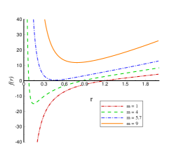
(a)  $n=4$ and $q=1$

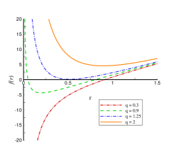
(b)  $n=3$ and $m=4$

Figure 1: The behavior of $f(r)$ versus $r$ for $\beta=2$, $m_{0}=4$ , $c_{0}=0.5$, $c_{1}=1$, $c_{2}=-0.4$, $c_{3}=0.4$ and $c_{4}=0.5$

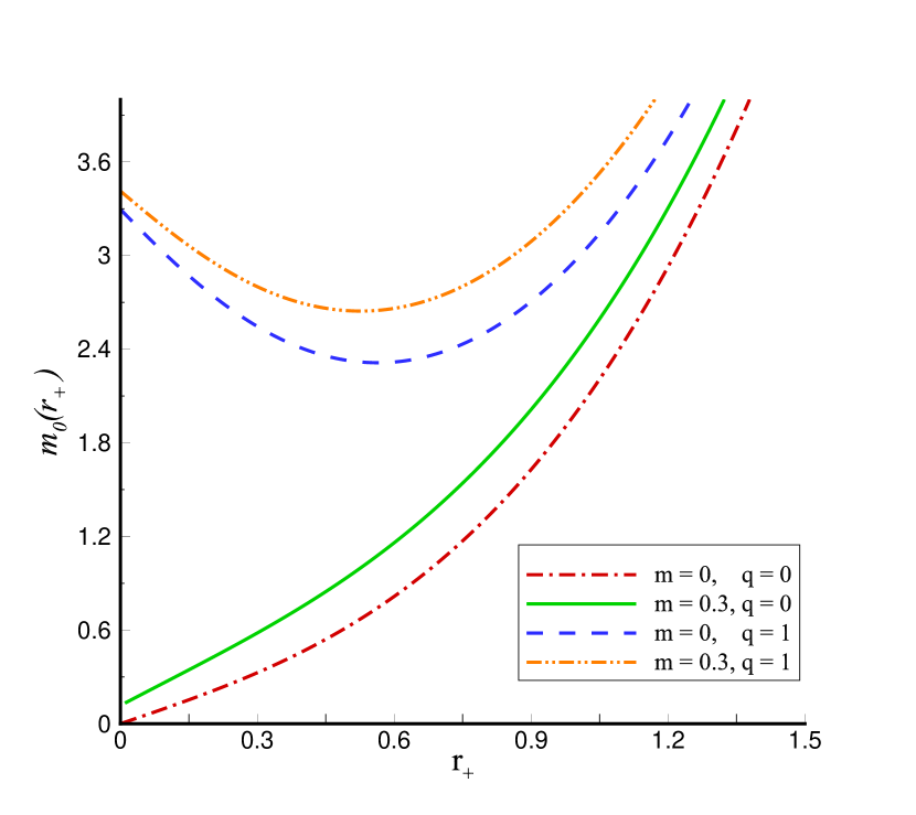
Figure 2: The behavior of $m_{0}(r_{+})$ versus $r_{+}$ for      $\beta=1$, $n=3$, $c_{0}=-1$, $c_{1}=c_{2}=6$, $c_{3}=1.3$ and $c_{4}=0.2$.

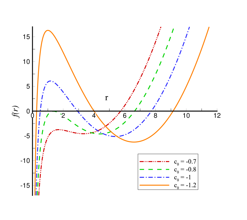
Figure 3: The behavior of $f(r)$ versus $r$ for $\beta=5$, $m_{0}=14.2$, $n=3$, $c_{1}=90$, $c_{2}=112$, $c_{3}=1.3$, $c_{4}=0.5$ and $m=0.5$.

We also choose $m_{0}$ as a constant of integration which is related to total mass of black hole. It is easy to obtain the parameter $m_{0}$ in (16) by using Eq. $f(r_{+})=0$. We find

$$m_{0} = kr_{+}^{n-2}-\frac{2r_{+}^{n}\Lambda}{n(n-1)}+\frac{8\beta^{2}r_{+}^{n}}{n\left(n-1\right)}\left[\ln\left(\frac{1+\Upsilon_{+}}{2}\right)+\frac{\left(2n-1\right)\left(1-\Upsilon_{+}\right)}{n}\right]$$ (18)

$$+\frac{8\left(n-1\right)q^{2}r_{+}^{-2n}}{n^{2}\left(n-2\right)}\mathbf{F}\left(\frac{1}{2},\frac{2-n}{2(-1+n)},\frac{4-3n}{2-2n},\frac{-q^{2}r_{+}^{2-2n}}{\beta^{2}}\right)$$

$$+\frac{c_{0}m^{2}r_{+}^{n-1}}{n-1}\left(c_{1}+\frac{(n-1)c_{0}c_{2}}{r_{+}}+\frac{(n-1)(n-2)c_{0}^{2}c_{3}}{r_{+}^{2}}+\frac{(n-1)(n-2)(n-3)c_{0}^{3}c_{4}}{r_{+}^{3}}\right),$$

in which $\Upsilon_{+}=\Upsilon(r_{+})$ and $r_{+}$ is the radius of horizon which is the largest root of $f(r_{+})=0$. As it is clear from Eq. (16), the position of $r_{+}$ completely depends on the metric parameters. This fact is shown in Fig. 1. In this figure, we set $l=k=1$. Depending on the number of metric function’s root(s), our solution may be a black hole with two inner and outer horizons, an extreme black hole or a naked singularity. As one can see from this figure, the number of horizons, decreases by increasing the massive gravity parameter $m$ and electric charge $q$. It is notable to mention that a suitable choice of metric parameters may result a Schwarzschild-like black hole (Fig. 1). From Fig. 3, we observe that in the presence of massive gravity and nonlinear electrodynamics, the mass parameter $m_{0}$ has non zero value when $r_{+}\rightarrow 0$. Fig. 3 also confirms the result of Fig. 1(b). Comparing dash-dotted and dashed as well as solid and dash-double-dotted curves in Fig. 3 shows that by increasing $q$ when $m$ is fix, we could move from Schwarzschild-like black holes with just one horizon to black holes with two horizons. One could also depict curves to show the same behavior for $m$ (as shown before in Fig. 1(a)), however we avoid this for economic reasons.

Fig. 3 represents a significant behavior of the metric function $f(r)$; the existence of several roots! The green (dashed) curve shows two roots where the smaller one is extreme and the blue (dash-dotted) curve exhibits the existence of three roots. Also, as one decreases the $c_{0}$ parameter, the largest root moves to larger values. Similar result has been reported in ref40 . It has been discussed that the physical reason behind this property is anti-evaporation ref40 . Anti-evaporation is a quantum effect which causes the size of black hole to increase.

The gauge potential $A_{t}$ can be calculated as

$$A_{t}\left(r\right) =\int F_{rt}dr$$

$$=\mu+\frac{2r^{n}\beta^{2}}{nq}\left(\Upsilon-1\right)+\frac{2\left(1-n\right)q^{2}r^{2-n}}{n\left(n-2\right)}\mathbf{F}\left(\frac{1}{2},\frac{n-2}{2(n-1)},\frac{4-3n}{2(1-n)},1-\Upsilon^{2}\right).$$ (19)

From holographic point of view, $\mu$ as a constant of integration is chemical potential of quantum field that locates on the boundary. It can be found by demanding the regularity condition on the horizon i.e. $A_{t}(r_{+})=0$

$$\mu=\frac{2r_{+}^{n}\beta^{2}}{nq}\left(1-\Upsilon_{+}\right)-\frac{2\left(1-n\right)q^{2}r_{+}^{2-n}}{n\left(n-2\right)}\mathbf{F}\left(\frac{1}{2},\frac{n-2}{2(n-1)},\frac{4-3n}{2(1-n)},1-\Upsilon_{+}^{2}\right).$$ (20)

We wind up this section by calculating the Hawking temperature on the event horizon

$$T = \frac{f^{\prime}(r_{+})}{4\pi}$$ (21)

$$= \frac{(n-2)k}{4\pi r_{+}}+\frac{m^{2}c_{0}}{4\pi r_{+}^{3}}\left(c_{0}^{3}c_{4}(n-4)(n-3)(n-2)+c_{0}^{2}c_{3}(n-3)(n-2)r_{+}+c_{0}c_{2}(n-2)r_{+}^{2}+c_{1}r_{+}^{3}\right)$$

$$-\frac{r_{+}\Lambda}{2\pi(n-1)}+\frac{2r_{+}\beta^{2}\left[\left(1-\Upsilon_{+}\right)+\ln\left(\frac{1}{2}\left(1+\Upsilon_{+}\right)\right)\right]}{\pi(n-1)}.$$

In the next section, we will study the thermodynamics of our black hole solutions.

III THERMODYNAMICS OF MASSIVE GRAVITY SOLUTIONS

In order to investigate the thermodynamics of our black hole solutions, we have to calculate some thermodynamical quantities. We first obtain the entropy of the black holes. Based on ref39 , this thermodynamic quantity is equal to one-quarter of the horizon area

$$S=\frac{r_{+}^{n-1}}{4}.$$ (22)

The Gauss law allows us to compute electric charge per unit volume $V_{n-1}$ using electromagnetic flux at infinity,

$$Q=\frac{\,{1}}{4\pi}\int r^{n-1}\left(1+\frac{\mathcal{F}}{8\beta^{2}}\right)^{-1}F_{\mu\nu}n^{\mu}u^{\nu}dr,$$ (23)

in which the unit spacelike and timelike normals to the hypersurface of radius $r$ are respectively $n^{\mu}=\left(\sqrt{-g_{tt}}\right)^{-1}dt=\left(\sqrt{f\left(r\right)}\right)^{-1}dt$ and $u^{\nu}=\left(\sqrt{g_{rr}}\right)^{-1}dr=\sqrt{f(r)}dr$. Finally, the electric charge per unit volume $V_{n-1}$ of black hole could be obtained as

$$Q=\frac{\,q}{4\pi}.$$ (24)

Electric potential can measure at infinity with respect to the horizon using the following definition

$$U=A_{\mu}\chi^{\mu}\left|{}_{r\rightarrow\infty}-A_{\mu}\chi^{\mu}\right|_{r=r_{+}},$$ (25)

where $\chi=\partial_{t}$ is the null generator of the horizon. So it is easy to show that electric potential is equal to chemical potential

$$U=\mu.$$ (26)

The mass of our charged solution using the Hamiltonian approach can be found as

$$M=\frac{(n-1)m_{0}}{16\pi}.$$ (27)

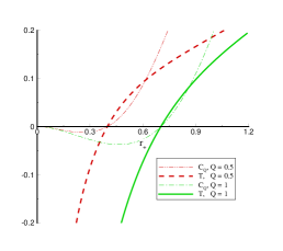
(a)  $m=5$

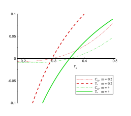
(b)  $q=0.5$

Figure 4: The behavior of $C_{Q}$ and $T$ versus $r_{+}$ for $\beta=1$, $m_{0}=0.2$, $n=3$, $c_{0}=-0.2$, $c_{1}=0.3$, $c_{2}=0.1$, $c_{3}=1.3$ and $c_{4}=5$.

Using (18), (22), (24) and (27), it is a matter of calculation to show that the mass function is

$$M(S,Q)= -\frac{\Lambda\,(4S)^{\frac{n}{n-1}}}{8n\pi}+\frac{m^{2}c_{0}}{16\pi}\left[(n-1)(n-2)(4S)^{\frac{n-3}{n-1}}\left(c_{3}+(4S)^{\frac{-1}{n-1}}(n-3)c_{4}\right)c_{0}^{3}+(4S)^{\frac{n-2}{n-1}}(n-1)c_{2}c_{0}+4Sc_{1}\right]$$

$$+\frac{\beta^{2}}{2n\pi}\ln\left[\frac{1}{2}+\frac{1}{2}\sqrt{1+\frac{Q^{2}\pi^{2}}{\beta^{2}S^{2}}\,}\right](4S)^{\frac{n}{n-1}}+\frac{8(n-1)^{2}\,Q^{2}\pi}{n^{2}(n-2)}\mathbf{F}\left(\frac{1}{2},\frac{n-2}{2n-2},\frac{3n-4}{2-2n},-\frac{Q^{2}\pi^{2}}{\beta^{2}S^{2}}\right)(4S)^{\frac{2-n}{n-1}}$$

$$+\frac{1}{16n^{2}\pi}\left[8\beta^{2}(2n-1)+k\,n^{2}(n-1)(4S)^{\frac{-2}{n-1}}-8\beta^{2}(2n-1)\sqrt{1+\frac{Q^{2}\pi^{2}}{\beta^{2}S^{2}}}\,\right](4S)^{\frac{n}{n-1}}$$ (28)

In order to check the validity of the first law of thermodynamics for our solutions, we consider entropy $S$ and electric charge $Q$ as a complete set of extensive quantities for mass. Also, we define temperature $T$ and electric potential $U$ as their conjugate intensive quantities, respectively:

$$T=\left(\frac{\partial M(S,Q)}{\partial S}\right)_{Q}\text{ \ \ \ \ and \ \ \ \ }U=\left(\frac{\partial M(S,Q)}{\partial Q}\right)_{S}.$$ (29)

Our numerical calculations show that, above quantities satisfy the first law of black hole thermodynamics:

$$dM=TdS+UdQ.$$ (30)

In following section, we will investigate the thermal stability of obtained solutions.

IV Thermal Stability

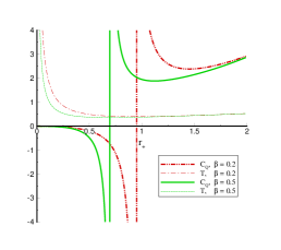
(a)  $n=3$, $c_{1}=4$, $c_{2}=10$, $c_{3}=13$, $c_{4}=0.5$, $q=1$, $m=0.5$

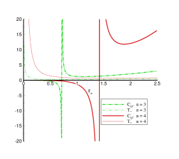
(b)  $\beta=0.4$, $c_{1}=3$, $c_{2}=2$, $c_{3}=2$, $c_{4}=1$, $q=0.5$, $m=0.8$

Figure 5: The behavior of $C_{Q}$ and $T$ versus $r_{+}$ for $m_{0}=2$ and $c_{0}=-1$.

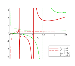
Figure 6: The behavior of $C_{Q}$ and $T$ versus $r_{+}$ for $\beta=3$, $m_{0}=2$, $n=3$, $c_{1}=1$, $c_{2}=3$, $c_{3}=1$, $c_{4}=-7$, $q=0.5$ and $m=1$.

This section is devoted to study the thermal stability of the obtained solutions. One can consider the stability of a black hole in both canonical and grand canonical ensembles. In canonical ensemble, positivity of the heat capacity together with the positive values for the temperature guaranties thermal stability of the solutions. Heat capacity is defined as

$$C_{Q}=T\left(\frac{\partial S}{\partial T}\right)_{Q}=\left(\frac{\partial M}{\partial S}\right)_{Q}\left(\frac{\partial^{2}M}{\partial S^{2}}\right)_{Q}^{-1}.$$ (31)

In case of unstable black hole, a phase transition occur to get stable state. We desire to investigate the phase transition point by finding the roots and divergencies of $C_{Q}$. The roots of heat capacity which are equivalent to zero values of temperature, determine a thermal transition between un-physical ($T<0$) and physical ($T>0$) state of the black hole. Beside, we recall that based on the thermal physics, when the heat capacity diverges, a second order phase transition will occur.

Since it is not easy to determine the roots and divergencies of the heat capacity analytically, we study this by using the figures. The behaviors of $C_{Q}$ in terms of $r_{+}$ for different sets of parameters have been depicted in Figs. 4-6. It is obvious that the stability depends on the metric parameters. By choosing a proper set of metric parameters, Fig. 4 specifies that by increasing the electric charge $Q$ (massive parameter $m$), the transition between un-physical and physical states will occur for larger black holes.

Fig. 5 illustrates a second order phase transition of our solutions for some specific values of the model parameters. The transition is between two physical states since the temperature is positive. In Fig. 5, we observe that for smaller black holes $C_{Q}$ is negative, so they are not stable and transition allows us to have larger stable black holes. In addition, as we decrease the nonlinearity of electrodynamics (larger $\beta$), the transition happens for smaller black holes (Fig. 5(a)). As Fig. 5(b) shows, for higher dimensions phase transition occurs for larger horizon radii.

Changing massive model parameters causes rich phase transitions (Fig. 6). The solid curve in Fig. 6 shows two transitions. One from stable small black hole to unstable middle black hole and another from unstable middle black hole to stable large black hole. These transitions represent that depending on the metric parameters, the middle black holes may not be allowed. This fact is clear from dash-double-dotted curve for which the transition is just from small to large black holes.

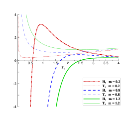
(a)  $c_{0}=-2$, $c_{2}=3$, $c_{4}=0.5$, $n=3$

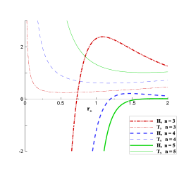
(b)  $c_{0}=-0.8$, $c_{2}=1$, $c_{4}=1$, $m=1.2$

Figure 7: The behavior of $\mathbf{H}$ and $T$ versus $r_{+}$ for $\beta=0.5$ , $m_{0}=2$, $c_{1}=1$, $c_{3}=1$ and $Q=0.5$.

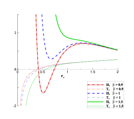
(a)  $Q=1.5$, $m_{0}=1$, $c_{2}=3$, $c_{3}=13$, $c_{4}=-1$, $m=1$

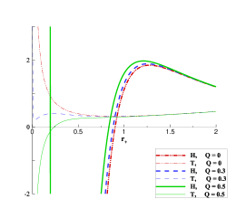
(b)  $\beta=2$, $m_{0}=2$, $c_{2}=1$, $c_{3}=2$, $c_{4}=1$, $m=1.2$

Figure 8: The behavior of $\mathbf{H}$ and $T$ versus $r_{+}$ for $n=3$, $c_{0}=-1$, $c_{1}=1$ and $c_{3}=1$.

Now, we turn to study the stability in the grand canonical ensemble. Basically, the local stability can be carried out by finding the determinant of the Hessian matrix $\mathbf{H}$ with respect to its extensive variables, $X_{i}$’s. In the canonical ensemble, $Q$ is a fixed parameter so the positivity of heat capacity ($C_{Q}$) is sufficient to ensure the local thermal stability. However, in grand canonical ensemble, the number of extensive parameters depends on the theory, and we have to check the sign of $\mathbf{H}$ to search for thermal stability. In our case, the mass is a function of extensive variables entropy $S$ and charge $Q$. So, Hessian matrix defines as

$$\mathbf{H}_{X_{i},X_{j}}^{M}=\frac{\partial^{2}M}{\partial X_{i}\partial X_{J}}=\left[\begin{array}[]{cc}\frac{\partial^{2}M}{\partial S^{2}}&\frac{\partial^{2}M}{\partial S\partial Q}\\ \frac{\partial^{2}M}{\partial S\partial Q}&\frac{\partial^{2}M}{\partial Q^{2}}\end{array}\right].$$ (32)

It is not easy to investigate the thermal stability analytically, so we turn to the figures again. The behavior of $\mathbf{H}$ in terms of $r_{+}$ for different sets of model parameters has been plotted in Fig. 7 and 8. By fixing other metric parameters, Fig.7(a) shows a minimum value for horizon radius that for values under which black holes are unstable. This minimum value grows with increasing the mass parameter of massive gravity. The same behavior could be seen as well in terms of dimension $n$ (Fig. 7(b)). We emphasize that in this range the temperature is positive.

Changing nonlinear parameter $\beta$, may create two roots for $\mathbf{H}$ (Fig. 8). But since the temperature is negative for smaller root, the only important limit for allowed horizon radius value depends on the larger root. As one can see from Fig. 8, the horizon of stable black hole should be larger than larger root. It is notable to mention that by increasing $\beta$ this limit is removed. We observe from Fig.8(b) that increasing electric charge $Q$ causes two roots for $\mathbf{H}$. We do not care to the smaller root since it places in the negative range of temperature. Furthermore, the larger root grows for smaller electric charges, so the stable black holes have larger horizons.

V Critical behavior and Reentrant phase transition

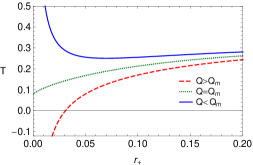
Figure 9: $T-r_{+}$ diagram of ($3+1$)-dimensional logarithmic charged massive black hole. We have set $c_{0}=1$, $c_{1}=1$, $c_{2}=-0.1$, $m=1$, $l=1$ and $\beta=1$.

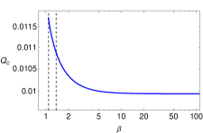
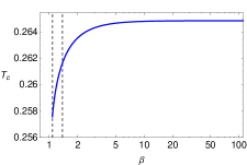
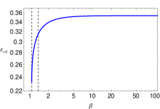
Figure 10: The behaviors of $Q_{c}$, $T_{c}$ and $r_{+c}$ vs $\beta$ with $c_{0}=0.5$, $c_{1}=1$, $c_{2}=-1$, $m=1$ and $l=1$. Note that the horizontal axes are logarithmic.

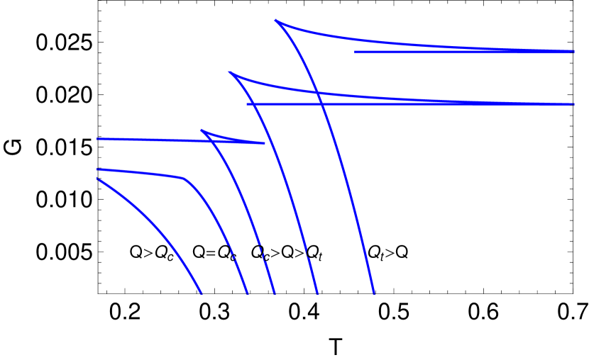
Figure 11: Gibbs free energy as a function of temperature for RN-type black holes with different values of charge. We fix $c_{0}=0.5$, $c_{1}=1$, $c_{2}=-1$, $m=1$, $l=1$ and $\beta=5$. Note that curves are shifted for clarity.

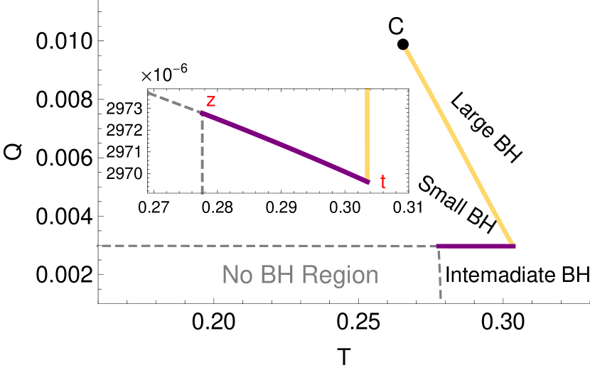
Figure 12: Phase diagram corresponding to RN-type black holes with $c_{0}=0.5$, $c_{1}=1$, $c_{2}=-1$, $m=1$, $l=1$ and $\beta=5$. Note that No BH region corresponds to no black hole solution for region of parameter space.

In this section, we first explore critical behavior of ($3+1$)-dimensional logarithmic charged massive black hole solutions with spherical event horizon ($k=1$) by investigating the behavior of the specific heat at constant charge, $C_{Q}$. Then, by studying Gibbs free energy $G$, we seek for different phase transitions of systems.

The specific heat at constant charge is defined as

$$C_{Q}=T\left(\frac{dS}{dT}\right)_{Q}.$$ (33)

The sign of $C_{Q}$ indicates the local thermodynamic stability/instability of the system. The positive (negative) sign of this quantity shows the local thermodynamic stability (instability). Note that Eq. (33) is also calculated at fixed cosmological constant and parameter of nonlinearity $\beta$. In Fig. 9, we plot the behavior of temperature with respect to event horizon radius for different values of the charge. The sign of slope in $T-r_{+}$ curves in allowed regions with positive temperature determines the sign of $C_{Q}$. Expanding the Hawking temperature (21) for small $r_{+}$, we receive

$$T=\frac{4\beta}{r_{+}}\left(Q_{m}-Q\right)+\frac{c_{0}c_{1}m^{2}}{4\pi}+\frac{r_{+}\left(3+4l^{2}\beta^{2}\left[1+\ln\left(2\pi Q/\beta\right)\right]\right)}{4\pi l^{2}}-\frac{2\beta^{2}r_{+}\ln\left(r_{+}\right)}{\pi}+O\left(r_{+}^{3}\right),$$ (34)

where $Q_{m}=\left(1+c_{0}^{2}c_{2}m^{2}\right)/\left(16\pi\beta\right)$ is the ‘marginal charge’ and we use $\Lambda=-3/l^{2}$. As one can see, the behavior of the temperature for small $r_{+}$ depends on the charge of the black hole. For $Q>Q_{m}$, black hole has zero temperature for a specific value of $r_{+}$ and for values greater than it temperature is positive. It means that these black holes are Reissner-Nordstrom (RN) type. For $Q<Q_{m}$, the black hole does not exist in low temperature region and temperature diverges as $r_{+}$ goes to zero (similar to Schwarzschild solution). So, these black holes are Schwarzschild (S) type. Note that for $Q=Q_{m}$, the black hole has a finite positive temperature as $r_{+}$ tends to zero. Therefore, the latter is neither S-type, nor RN-type and is marginal. This is the effect of massive term $c_{0}c_{1}m^{2}/4\pi$ in (34). For massless case ($m=0$), $T\rightarrow 0$ as $r_{+}\rightarrow 0$ for $Q=Q_{m}$ and the black hole is RN-type 1711.01151 . The large $r_{+}$ limit of the temperature is $3r_{+}/4\pi l^{2}$ which is clearly independent of the charge and increases linearly as $r_{+}$ increases (see Fig. 9).

Now, we intend to obtain the critical point (where continuous phase transition occurs). In order to characterize the critical point, we have

$$\frac{\partial T}{\partial S}\Big{|}_{Q_{c}}=0,\quad\quad\quad\frac{\partial^{2}T}{\partial S^{2}}\Big{|}_{Q_{c}}=0,$$ (35)

where $Q_{c}$ is the critical charge. Using (35), one could determine $Q_{c}$ and $r_{+c}$ and specify the critical point ($Q_{c},T_{c},r_{+c}$). In Fig. 10, we plot the behavior of $Q_{c}$, $T_{c}$ and $r_{+c}$ with respect to $\beta$ for a set of model parameters by solving the equations of (35) numerically. The vertical dashed lines in Fig. 10 show the range in which the critical behavior takes place for S-type black holes. For $\beta$ values larger than one specified by the rightmost vertical dashed line, the critical point occurs for RN-type black holes.

Now, we turn to study the behavior of Gibbs free energy for our black holes to find out the phase structure of the system. It determines the globally stable state at equilibrium process. The lowest Gibbs free energy specifies the global stable state. One could obtain the Gibbs free energy per unit volume $V_{2}$ as RPT1

$$G=M-TS,$$ (36)

We focus on RN-type ($3+1$)-dimensional logarithmic charged massive black holes. The Gibbs free energy as a function of temperature for different values of charge is illustrated in Fig. 12. In addition, the phase diagram is depicted in the $Q$–$T$ diagram in Figs. 12. According to the value of charge $Q$, we have different phase transitions. For $Q=Q_{c}$, the system is at critical point. This point is highlighted by a black spot in Fig. 12. For charge values greater than $Q_{c}$, the system is locally stable ($C_{Q}>0$) and Gibbs free energy is single valued. Therefore, no phase transition happens. For charge values less than critical value $Q_{c}$, there are thermally instable phases in the system ($C_{Q}<0$). So, the system experiences different phase transitions depending on the value of charge $Q$. A first order phase transition between small and large black holes occurs for $Q_{z}<Q<Q_{c}$. This is accompanied by a discontinuity in the slope of Gibbs free energy at transition point. This phase transition is marked by the gold curve in Fig. 12. For $Q$ in the range of $Q_{t}<Q<Q_{z}$, an interesting phenomenon happens. In this range, in addition to a first order phase transition which sepatates small and large black holes, a zeroth order phase transition between small and intermediate black holes occurs. This can be seen as a finite jump in Gibbs free energy in Fig. 12. The latter initiates from $Q=Q_{z}$ and terminates at $Q=Q_{t}$. $z$ and $t$ points are specified in Fig. 12. In this figure, this zeroth order phase transition is identified by purple curve. This intermediate (large)/small/large transition shows a reentrant phase transition RPT1 ; RPT2 . This is the first observation of reentrant phase transition for black hole solutions in massive gravity without extending thermodynamics phase space. In RPT3 , the occurance of reentrant phase transition in extended thermodynamics phase space has been reported for black holes in massive gravity. As Fig. 12 exhibits, no phase transition happens for $Q<Q_{t}$ and only stable large black holes exists. Also, no black hole region in Fig. 12 corresponds to no black hole solution exists.

VI Summary and CLOSING REMARKS

The importance of massive gravity model is at least twofold. On the one hand, because of the recent developments in gravitational waves observatory indicating the speed of gravitational wave deviates from the speed of light which implies the existence of massive graviton, we need an extension of general relativity with a massive graviton as intermediate particle similar to $W$ and $Z$ in electroweak interaction. On the other hand, from holographic viewpoint, giving mass to gravity could model momentum dissipation in dual system on boundary. In this work, we have studied black hole solutions in massive gravity model in the presence of LNE Lagrangian. As well as BI model, in the logarithmic one, there is no divergency in the electric field of a point particle at the origin.

We first constructed the field equations by varying the action. Then, we obtained the exact solution of the metric function and studied the behavior of the obtained solutions. We observed that depending on the model parameters, it is possible to have two horizons, an extreme horizon, or naked singularity. Moreover, one of the effects of massive gravity is the existence of multi horizons. This phenomenon is due to anti-evaporation which is a quantum effect. Next, we calculated the conserved and thermodynamic quantities. Calculation of these quantities is necessary for checking the satisfaction of the first law of black hole thermodynamics. It was observed that in the presence of nonlinear electrodynamics and within the context of massive gravity model, the first law of thermodynamic is still valid.

We studied the thermal stability in both canonical and grand canonical ensembles. We observed that considering different values for the model parameters leads to a variety of phase structures for our black holes. In canonical ensemble, the heat capacity can experience both positive and negative values. The position of its root(s) and divergency(ies) affected by metric parameters. In this ensemble, our black holes encounter two types of phase transitions; the second order phase transition in the position of divergences of heat capacity with positive temperature, and transitions between un-physical ($T<0$) and physical ($T>0$) states of solutions. Increasing the values of electric charge ($Q$) or massive parameter ($m$) causes the transition between un-physical and physical black holes in larger sizes (Fig. 4). It means that there is a lower bound on black hole radius increased as $Q$ and $m$ are enhanced. Also, by decreasing the nonlinearity parameter ($\beta$), second order phase transition happens for smaller black holes (Fig. 5). In the grand canonical ensemble, the determinant of the Hessian matrix $\mathbf{H}$ had a root with positive temperature, which its value depends on the metric parameters. We found out that some horizon radii are not allowed for our solution since $\mathbf{H}$ is negative for them. For instance, when other parameters are fixed, the stability is observed for larger black hole when massive parameter $m$ (or dimension $n$) increases (Fig. 7). Also, for smaller values of electric charge, the stability is guaranteed for larger black holes (Fig. 8).

Finally, we investigated the critical behavior of ($3+1$)-dimensional black holes with spherical event horizon. We showed that there is a marginal charge $Q_{m}$ that for charge values greater than it black holes are Reissner-Nordstrom-type, whereas for charge values less than it black holes are Schwarzschild-type. For massless gravity, the black hole solutions with $Q=Q_{m}$ are RN-type. We observed that in the context of massive gravity the latter are neither S-type nor RN-type and have a marginal behavior due to the effects of massive term. Next, we focused on RN-type black holes and study the behavior of Gibbs free energy to disclose the phase structure of solutions. We found out that there are different phase transitions according to the value of charge $Q$. There are some ranges for which there is no phase transition. However, for another range we just have a first order phase transition between small and large black holes accompined by a discontinuity in the slope of Gibbs free energy at transition point. Interestingly enough, there is a range of charge values for which black holes experience a zeroth order phase transition where a finite jump in Gibbs free energy value occurs. This causes a reentrant phase transition i.e. a large/small/large phase transition. This is the first report of reentrant phase transition for black holes in massive gravity without needing to extend thermodynamics phase space.

The study of this work can be extended from differnt aspects. For instance, in this context, one could explore the behavior of holographic conductivity. Furthermore, the effects of massive gravity with logarithmic electrodynamics on holographic superconductors could be investigated. Here, we examined the critical behavior of ($3+1$)-dimensional black holes numerically. This may be studied analytically. Also, one could explore this behavior for higher dimensional black holes. Moreover, the effects of more model parameters on phase behavior of such systems could be taken under study. Some of these pointed out issues are now under investigation.