Spectral decomposition of discrepancy kernels on the Euclidean ball, the special orthogonal group, and the Grassmannian manifold

Abstract.

To numerically approximate Borel probability measures by finite atomic measures, we study the spectral decomposition of discrepancy kernels when restricted to compact subsets of $\mathbb{R}^{d}$. For restrictions to the Euclidean ball in odd dimensions, to the rotation group $\operatorname*{SO}(3)$, and to the Grassmannian manifold $\operatorname{\mathcal{G}}_{2,4}$, we compute the kernels’ Fourier coefficients and determine their asymptotics. The $L_{2}$-discrepancy is then expressed in the Fourier domain that enables efficient numerical minimization based on the nonequispaced fast Fourier transform. For $\operatorname*{SO}(3)$, the nonequispaced fast Fourier transform is publicly available, and, for $\operatorname{\mathcal{G}}_{2,4}$, the transform is derived here. We also provide numerical experiments for $\operatorname*{SO}(3)$ and $\operatorname{\mathcal{G}}_{2,4}$.

1. Introduction

Consider a Borel probability measure $\mu:\mathscr{B}(\mathbb{R}^{d})\rightarrow[0,1]$ on $\mathbb{R}^{d}$, where $\mathscr{B}(\mathbb{R}^{d})$ denotes the Borel sigma algebra on $\mathbb{R}^{d}$. For fixed $n\in\mathbb{N}$, we aim to allocate a suitable $n$-point set $\{x_{1},\ldots,x_{n}\}\subset\mathbb{R}^{d}$ such that the normalized atomic measure

(1.1) $$\nu_{n}:=\frac{1}{n}\sum_{j=1}^{n}\delta_{x_{j}}$$

approximates $\mu$. Here, $\delta_{x_{j}}:\mathscr{B}(\mathbb{R}^{d})\rightarrow\{0,1\}$ denotes the point measure localized at $x_{j}$. To quantify the $L_{2}$-discrepancy between $\mu$ and $\nu_{n}$, select a measure $\beta$ on $\mathscr{B}(\mathbb{R}^{d})$ with $\mu,\delta_{x}\in L_{2}(\mathscr{B}(\mathbb{R}^{d}),\beta)$, for all $x\in\mathbb{R}^{d}$, and consider

(1.2) $$\mathscr{D}_{\beta}(\mu,\nu_{n}):=\|\mu-\nu_{n}\|^{2}_{L_{2}(\mathscr{B}(\mathbb{R}^{d}),\beta)}=\int_{\mathscr{B}(\mathbb{R}^{d})}\left|\mu(B)-\nu_{n}(B)\right|^{2}{\rm d}\beta(B),$$

cf. [40, 42, 43], see Section 2 for explicit examples. For fixed $n\in\mathbb{N}$, we aim to minimize $\mathscr{D}_{\beta}(\mu,\nu_{n})$ among all $n$-point sets $\{x_{1},\ldots,x_{n}\}\subset\mathbb{R}^{d}$. The present manuscript is concerned with discretizations of (1.2) that facilitate numerical minimization.

The associated discrepancy kernel $K_{\beta}:\mathbb{R}^{d}\times\mathbb{R}^{d}\rightarrow\mathbb{R}$ is defined by

(1.3) $$K_{\beta}(x,y):=\langle\delta_{x},\delta_{y}\rangle_{L_{2}(\mathscr{B}(\mathbb{R}^{d}),\beta)}=\int_{\mathscr{B}(\mathbb{R}^{d})}\delta_{x}(B)\delta_{y}(B){\rm d}\beta(B),$$

and we assume it is continuous. Fubini’s Theorem and $\mu(B)=\int_{\mathbb{R}^{d}}\delta_{x}(B){\rm d}\mu(x)$ applied to

$$\|\mu-\nu_{n}\|^{2}_{L_{2}(\mathscr{B}(\mathbb{R}^{d}),\beta)}=\|\mu\|^{2}_{L_{2}(\mathscr{B}(\mathbb{R}^{d}),\beta)}-2\langle\mu,\nu_{n}\rangle_{L_{2}(\mathscr{B}(\mathbb{R}^{d}),\beta)}+\|\nu_{n}\|^{2}_{L_{2}(\mathscr{B}(\mathbb{R}^{d}),\beta)}$$

yields that (1.2) is identical to

(1.4) $$\mathscr{D}_{\beta}(\mu,\nu_{n})=\iint\limits_{\mathbb{R}^{d}\times\mathbb{R}^{d}}K_{\beta}(x,y){\rm d}\mu(x){\rm d}\mu(y)-2\sum_{j=1}^{n}\int_{\mathbb{R}^{d}}\frac{K_{\beta}(x,x_{j})}{n}{\rm d}\mu(x)+\sum_{i,j=1}^{n}\frac{K_{\beta}(x_{i},x_{j})}{n^{2}}.$$

If a compact set $\mathbb{X}\subset\mathbb{R}^{d}$ is known in advance such that $\textnormal{supp}(\mu)\subset\mathbb{X}$, then we shall restrict the minimization to $\{x_{1},\ldots,x_{n}\}\subset\mathbb{X}$, so that only the restricted kernel $K_{\beta}|_{\mathbb{X}\times\mathbb{X}}$ matters. By endowing $\mathbb{X}$ with a finite Borel measure $\sigma_{\mathbb{X}}$ having full support, Mercer’s Theorem yields an orthonormal basis $\{\phi_{l}\}_{l=0}^{\infty}$ for $L_{2}(\mathbb{X},\sigma_{\mathbb{X}})$ and coefficients $(a_{l})_{l=0}^{\infty}$ such that the spectral decomposition

(1.5) $$K_{\beta}|_{\mathbb{X}\times\mathbb{X}}(x,y)=\sum_{l=0}^{\infty}a_{l}\phi_{l}(x)\overline{\phi_{l}(y)},\quad x,y\in\mathbb{X},$$

holds with absolute and uniform convergence. We call $(a_{l})_{l=0}^{\infty}$ the Fourier coefficients of the kernel $K_{\beta}|_{\mathbb{X}\times\mathbb{X}}$. If $\textnormal{supp}(\mu),\textnormal{supp}(\nu_{n})\subset\mathbb{X}$, then the Fourier expansion of the $L_{2}$-discrepancy (1.4) is

(1.6) $$\mathscr{D}_{\beta}(\mu,\nu_{n})=\sum_{l=0}^{\infty}a_{l}\left|\hat{\mu}_{l}-\hat{\nu}_{n,l}\right|^{2},\qquad\hat{\mu}_{l}:=\int_{\mathbb{X}}\overline{\phi_{l}(x)}{\rm d}\mu(x),\quad\hat{\nu}_{n,l}:=\frac{1}{n}\sum_{j=1}^{n}\overline{\phi_{l}(x_{j})},$$

where the Fourier coefficients $\hat{\mu}_{l}$ and $\hat{\nu}_{n,l}$ of the measures $\mu$ and $\nu_{n}$, respectively, are well-defined if $a_{l}\neq 0$. Truncation of the discretization (1.6) enables the use of the nonequispaced fast Fourier transform, thereby offering more efficient minimization of $\mathscr{D}_{\beta}(\mu,\nu_{n})$, cf. [31, 33]. Thus, we aim to

A) compute $(a_{l})_{l=0}^{\infty}$ and $(\phi_{l})_{l=0}^{\infty}$ in the Fourier expansion (1.5) of $K_{\beta}|_{\mathbb{X}\times\mathbb{X}}$.

The $L_{2}$-discrepancy $\mathscr{D}_{\beta}(\mu,\nu_{n})$ also coincides with the worst case integration error

(1.7) $$\mathscr{D}_{\beta}(\mu,\nu_{n})=\sup_{\|f\|_{\mathscr{H}_{\beta}(\mathbb{X})}\leq 1}\left|\int_{\mathbb{X}}f(x){\rm d}\mu(x)-\frac{1}{n}\sum_{j=1}^{n}f(x_{j})\right|^{2}$$

with respect to the reproducing kernel Hilbert space $\mathscr{H}_{\beta}(\mathbb{X})$ generated by $K_{\beta}|_{\mathbb{X}\times\mathbb{X}}$, cf. [12, 13, 29, 31]. To specify $\mathscr{H}_{\beta}(\mathbb{X})$, we aim to

B) identify $\mathscr{H}_{\beta}(\mathbb{X})$ with a classical function space.

Fourier decay properties generally quantify Sobolev smoothness. To accomplish B), we aim to determine the asymptotics of $K_{\beta}|_{\mathbb{X}\times\mathbb{X}}$’s Fourier coefficients $(a_{l})_{l=0}^{\infty}$ in (1.5).

For $\mathbb{X}=\mathbb{S}^{d-1}$ and a particular choice of $\beta$, the kernel $K_{\beta}|_{\mathbb{S}^{d-1}\times\mathbb{S}^{d-1}}$ essentially coincides with the Euclidean distance, see [12, 13]. The Fourier expansion is determined in [10], and the decay of the Fourier coefficients yields that $K_{\beta}|_{\mathbb{S}^{d-1}\times\mathbb{S}^{d-1}}$ reproduces the Sobolev space $\mathscr{H}_{\beta}(\mathbb{S}^{d-1})=\mathbb{H}^{\frac{d}{2}}(\mathbb{S}^{d-1})$. For the sphere and the torus, the nonequispaced fast Fourier transform is available, and both A) and B) are discussed in [33, 34].

This manuscript is dedicated to derive analogous results for other compact sets $\mathbb{X}$. We focus on the unit ball, the special orthogonal group, and the Grassmannian manifold,

$$\mathbb{B}^{d} :=\{x\in\mathbb{R}^{d}:\|x\|\leq 1\},$$

$$\operatorname*{SO}(d) :=\{x\in\mathbb{R}^{d\times d}:\det(x)=1,\,x^{-1}=x^{\top}\},$$

$$\mathcal{G}_{k,d} :=\{x\in\mathbb{R}^{d\times d}:x^{\top}=x,\,x^{2}=x,\,\operatorname*{trace}(x)=k\}.$$

We achieve goal A) for $\mathbb{X}=\mathbb{B}^{d}$ with odd $d$. Both goals, A) and B), are achieved for $\operatorname*{SO}(3)$ and $\operatorname{\mathcal{G}}_{2,4}$. We also provide numerical experiments. For $\operatorname*{SO}(3)$, the computations are based on the nonequispaced fast Fourier transform designed in [32, 44]. For $\operatorname{\mathcal{G}}_{2,4}$, we derive the nonequispaced fast Fourier transform by parametrization via the double covering $\mathbb{S}^{2}\times\mathbb{S}^{2}$ and developing the respective transform there. We also accomplish B) for the general cases $\operatorname*{SO}(d)$ and $\operatorname{\mathcal{G}}_{k,d}$.

2. Two introductory examples

We first present a well-known elementary example on the interval $[0,s]$, for which both aims A) and B) are achieved. Second, to support our perspective on discrepancy, we prove that the so-called Askey function is a discrepancy kernel of the form (1.3).

2.1. The Brownian motion kernel on $[0,s]$

Let ${\rm d}r$ be the Lebesgue measure on $[0,\infty)$. The mapping $h:[0,\infty)\rightarrow\mathscr{B}(\mathbb{R})$ defined by $r\mapsto[r,\infty)$ induces the pushforward measure $\beta:=h_{*}({\rm d}r)$ that induces the discrepancy

$$\mathscr{D}_{\beta}(\mu,\nu_{n})=\int_{0}^{\infty}|\mu([r,\infty))-\nu_{n}([r,\infty))|^{2}{\rm d}r.$$

The associated discrepancy kernel $K_{\beta}:\mathbb{R}\times\mathbb{R}\rightarrow\mathbb{R}$ is

$$K_{\beta}(x,y)=\int_{0}^{\infty}\delta_{x}([r,\infty))\delta_{y}([r,\infty)){\rm d}r=\min(x,y)_{+},$$

so that $\mathscr{D}_{\beta}(\delta_{x},\delta_{y})=|x-y|$ for $x,y\in[0,\infty)$. The restriction of the kernel $K_{\beta}$ to $[0,s]\times[0,s]$ has the Fourier expansion

$$K_{\beta}(x,y) =\sum_{\begin{subarray}{c}m\in\mathbb{N}\\ m\text{ odd}\end{subarray}}\frac{4s^{2}}{m^{2}\pi^{2}}\cdot\frac{\sin(\frac{\pi}{2s}mx)}{\sqrt{\frac{s}{2}}}\cdot\frac{\sin(\frac{\pi}{2s}my)}{\sqrt{\frac{s}{2}}},\quad x,y\in[0,s],$$

with respect to the Lebesgue measure $\sigma_{[0,s]}$ on $[0,s]$. The reproducing kernel Hilbert space is

$$\mathscr{H}_{K_{\beta}}([0,s])=\{f:[0,s]\rightarrow\mathbb{C}\;:\;f\text{ is absolutely continuous, }f(0)=0,\;f^{\prime}\in L_{2}([0,s])\},$$

where the inner product between $f$ and $g$ is given by $\langle f^{\prime},g^{\prime}\rangle_{L_{2}([0,s])}$, cf. [3, 21] and [43, Section 9.5.5]. Note that $K_{\beta}|_{[0,1]\times[0,1]}$ is often called the Brownian motion kernel and $\mathscr{H}_{K_{\beta}}([0,s])$ is continuously embedded into the Sobolev space $\mathbb{H}^{1}([0,s])$.

2.2. Askey’s function and its restrictions

Many positive definite kernels in the literature are of the form (1.3) and, hence, are discrepancy kernels. For odd $d$, Askey’s kernel function $(x,y)\mapsto(1-\|x-y\|)^{\frac{d+1}{2}}_{+}$ is positive definite, cf. [28]. In the following, we shall check that it is of the form (1.3).

Denote the Euclidean ball of radius ${s}$ centered at $z\in\mathbb{R}^{d}$ by

$$\mathbb{B}^{d}_{s}(z):=\{x\in\mathbb{R}^{d}:\|x-z\|\leq{s}\},$$

with the conventions $\mathbb{B}^{d}_{s}:=\mathbb{B}^{d}_{s}(0)$ and $\mathbb{B}^{d}:=\mathbb{B}^{d}_{1}$. Fix $r>0$ and consider the discrepancy

(2.1) $$\mathscr{D}_{d,r}(\mu,\nu_{n}):=\frac{1}{\operatorname*{vol}(\mathbb{B}^{d}_{\frac{r}{2}})}\int_{\mathbb{R}^{d}}\left|\mu(\mathbb{B}^{d}_{\frac{r}{2}}(z))-\nu_{n}(\mathbb{B}^{d}_{\frac{r}{2}}(z))\right|^{2}{\rm d}z,$$

where $\operatorname*{vol}(\mathbb{B}^{d}_{\frac{r}{2}})=\frac{\pi^{d/2}}{\Gamma(\frac{d}{2}+1)}(\frac{r}{2})^{d}$. The associated discrepancy kernel is

(2.2) $$K_{d,r}(x,y)=\frac{1}{\operatorname*{vol}(\mathbb{B}^{d}_{\frac{r}{2}})}\int_{\mathbb{R}^{d}}\delta_{x}(\mathbb{B}^{d}_{\frac{r}{2}}(z))\delta_{y}(\mathbb{B}^{d}_{\frac{r}{2}}(z)){\rm d}z.$$

In order to additionally integrate over $r$, recall the (generalized) hypergeometric functions

$${}_{k}F_{l}{\left(\genfrac{.}{.}{0.0pt}{}{f_{1},\ldots,f_{k}}{g_{1},\ldots,g_{l}};z\right)}:=\sum_{n=0}^{\infty}\frac{(f_{1})_{n}\cdots(f_{k})_{n}}{(g_{1})_{n}\cdots(g_{l})_{n}}\frac{z^{n}}{n!},$$

where $f_{1},\ldots,f_{k},g_{1},\ldots,g_{l},z\in\mathbb{R}$ and $(f)_{n}:=f\cdot(f+1)\cdots(f+n-1)$ denotes the Pochhammer symbol with $(f)_{0}:=1$. We consider $G_{d}:[0,\infty)\rightarrow\mathbb{R}$ given by

$$G_{d}(r)=\begin{cases}{}_{2}F_{1}{\left(\genfrac{.}{.}{0.0pt}{}{-\frac{d+1}{4},-\frac{d-1}{4}}{-\frac{d}{2}};r^{2}\right)},&0\leq r\leq 1,\\ 0,&1<r.\end{cases}$$

Since $d$ is odd, either $\frac{d+1}{4}$ or $\frac{d-1}{4}$ is a natural number, so that the series terminates and $G_{d}$ is a polynomial in $r^{2}$ on $[0,1]$. By integration with respect to $G_{d}$, we obtain the $L_{2}$-discrepancy and the associated discrepancy kernel

$$\mathscr{D}_{d}(\mu,\nu_{n}):=\int_{0}^{\infty}\!\!\mathscr{D}_{d,r}(\mu,\nu_{n}){\rm d}G_{d}(r),\quad\text{ and }\quad K_{d}(x,y)=\int_{0}^{\infty}\!K_{d,r}(x,y){\rm d}G_{d}(r),$$

respectively. It turns out that $K_{d}$ coincides with Askey’s function.

Theorem 2.1.

Let $d$ be odd. The discrepancy kernel $K_{d}$ satisfies

(2.3) $$K_{d}(x,y)=(1-\|x-y\|)^{\frac{d+1}{2}}_{+},\quad x,y\in\mathbb{R}^{d}.$$

The proof is presented in Appendix A. Provided that $d\geq 3$, Askey’s kernel function reproduces the Sobolev space $\mathbb{H}^{\frac{d+1}{2}}(\mathbb{R}^{d})$ with an equivalent norm, see [49].

3. The distance kernel on $\mathbb{S}^{d-1}$

This section is dedicated to recall results on discrepancy kernels on the sphere $\mathbb{S}^{d-1}\subset\mathbb{R}^{d}$, for $d\geq 2$, from [12, 13, 31, 46] that shall guide our subsequent investigations.

Denote the geodesic ball of radius $r$ centered at $z\in\mathbb{S}^{d-1}$ by

$$B^{\mathbb{S}^{d-1}}_{r}(z):=\{x\in\mathbb{S}^{d-1}:\operatorname{dist}_{\mathbb{S}^{d-1}}(x,z)\leq r\},$$

where $\operatorname{dist}_{\mathbb{S}^{d-1}}(x,z)=\arccos(\langle x,z\rangle)$ is the geodesic distance on $\mathbb{S}^{d-1}$. We define

$$h:[0,\pi]\times\mathbb{S}^{d-1}\rightarrow\mathscr{B}(\mathbb{R}^{d}),\qquad(r,z)\mapsto B^{\mathbb{S}^{d-1}}_{r}(z)$$

and endow $[0,\pi]$ with the weighted Lebesgue measure $\sin(r){\mathrm{d}}r$, whereas $\mathbb{S}^{d-1}$ carries the normalized, orthogonal invariant surface measure $\sigma_{\mathbb{S}^{d-1}}$. The push-forward $\beta_{d}:=h_{*}(\sin(r){\mathrm{d}}r\otimes\sigma_{\mathbb{S}^{d-1}})$ is a measure on $\mathscr{B}(\mathbb{R}^{d})$, so that the associated $L_{2}$-discrepancy is

$$\mathscr{D}_{\beta_{d}}(\mu,\nu_{n})=\int_{0}^{\pi}\int_{\mathbb{S}^{d-1}}|\mu(B^{\mathbb{S}^{d-1}}_{r}(z))-\nu_{n}(B^{\mathbb{S}^{d-1}}_{r}(z))|^{2}{\rm d}\sigma_{\mathbb{S}^{d-1}}(z)\sin(r){\rm d}r.$$

The associated discrepancy kernel is

(3.1) $$K_{\beta_{d}}(x,y)=\int_{0}^{\pi}\int_{\mathbb{S}^{d-1}}\delta_{x}(B^{\mathbb{S}^{d-1}}_{r}(z))\delta_{y}(B^{\mathbb{S}^{d-1}}_{r}(z)){\rm d}\sigma_{\mathbb{S}^{d-1}}(z)\sin(r){\rm d}r,\quad x,y\in\mathbb{R}^{d}.$$

According to [12, 13, 31], see also [2], $K_{\beta_{d}}$ satisfies

(3.2) $$K_{\beta_{d}}(x,y)=1-\frac{\Gamma(\frac{d}{2})}{2\sqrt{\pi}\Gamma(\frac{d+1}{2})}\|x-y\|,\qquad x,y\in\mathbb{S}^{d-1}.$$

If either $x$ or $y$ is not contained in $\mathbb{S}^{d-1}$, then $K_{\beta_{d}}(x,y)=0$.

Choose $\sigma_{\mathbb{X}}:=\sigma_{\mathbb{S}^{d-1}}$ for the decomposition (1.5) and let $\{Y^{m}_{{l}}:l=1,\ldots,Z(d,m)\}\subset L_{2}(\mathbb{S}^{d-1},\sigma_{\mathbb{S}^{d-1}})$ denote the set of orthonormal spherical harmonics of degree $m$ on $\mathbb{S}^{d-1}$, where $Z(d,m)=\frac{2m+d-2}{d-2}\binom{m+d-3}{m}.$ For $\tau>(d-1)/2$, the Sobolev space $\mathbb{H}^{\tau}(\mathbb{S}^{d-1})$ is the reproducing kernel Hilbert space associated with the reproducing kernel

(3.3) $$(x,y)\mapsto\sum_{m=0}^{\infty}(1+m(m+d-2))^{-\tau}\sum_{l=1}^{Z(d,m)}Y^{m}_{l}(x)\overline{Y^{m}_{l}(y)},\quad x,y\in\mathbb{S}^{d-1}.$$

The coefficients in the Fourier expansion

$$1-\frac{\Gamma(\frac{d}{2})}{2\sqrt{\pi}\Gamma(\frac{d+1}{2})}\|x-y\|=\sum_{m=0}^{\infty}c_{m}\sum_{l=1}^{Z(d,m)}Y^{m}_{l}(x)\overline{Y^{m}_{l}(y)},\quad x,y\in\mathbb{S}^{d-1},$$

satisfy $|c_{m}|\sim m^{-d}$, cf. [12]. This is the same asymptotics as the coefficients in (3.3) for $s=d/2$. Therefore, $K_{\beta_{d}}|_{\mathbb{S}^{d-1}\times\mathbb{S}^{d-1}}$ reproduces the Sobolev space $\mathscr{H}_{\beta_{d}}(\mathbb{S}^{d-1})=\mathbb{H}^{\frac{d}{2}}(\mathbb{S}^{d-1})$ with an equivalent norm.

In order to determine the Fourier coefficients of kernels on the sphere that are polynomial in $\|x-y\|$, such as $K_{\beta_{d}}|_{\mathbb{S}^{d-1}\times\mathbb{S}^{d-1}}$, we require the Fourier coefficients of the monomial terms $\|x-y\|^{p}$. For any $p\in\mathbb{N}$, the Fourier expansion

(3.4) $$2^{-\frac{p}{2}}\|x-y\|^{p}=\sum_{m=0}^{\infty}a_{m}(p,\mathbb{S}^{d-1})\sum_{l=1}^{Z(d,m)}Y^{m}_{l}(x)\overline{Y^{m}_{l}(y)},\quad x,y\in\mathbb{S}^{d-1},$$

holds with coefficients determined by

(3.5) $$a_{m}(p,\mathbb{S}^{d-1}):=\iint\limits_{\mathbb{S}^{d-1}\times\mathbb{S}^{d-1}}2^{-\frac{p}{2}}\|x-y\|^{p}\overline{Y^{m}_{l}(x)}Y^{m}_{l}(y){\rm d}\sigma_{\mathbb{S}^{d-1}}(x){\rm d}\sigma_{\mathbb{S}^{d-1}}(y).$$

Note that (3.5) is well-defined for the entire range $p>-(d-1)$ and $p$ is not required to be an integer. For $p>0$, the following proposition is essentially due to [10], see also [12, 14]. Simple continuation arguments cover the full range of $p$, and the asymptotics $\frac{\Gamma(-\frac{p}{2}+m)}{\Gamma(\frac{p}{2}+d-1+m)}=m^{-(p+d-1)}(1+o(1))$ are standard.

Proposition 3.1 ([10]).

Suppose $d\geq 2$. For any $p>-(d-1)$, we have

(3.6) $$a_{m}(p,\mathbb{S}^{d-1}) =\frac{2^{d}\Gamma(\frac{d}{2})}{4\sqrt{\pi}}\cdot\frac{2^{p/2}\Gamma(\frac{d}{2}+\frac{p}{2}-\frac{1}{2})}{\Gamma(-\frac{p}{2})}\cdot\frac{\Gamma(-\frac{p}{2}+m)}{\Gamma(\frac{p}{2}+d-1+m)}.$$

In particular, if $p\not\in 2\mathbb{N}$, then

(3.7) $$|a_{m}(p,\mathbb{S}^{d-1})| =\left|\frac{2^{d}\Gamma(\frac{d}{2})}{4\sqrt{\pi}}\cdot\frac{2^{p/2}\Gamma(\frac{d}{2}+\frac{p}{2}-\frac{1}{2})}{\Gamma(-\frac{p}{2})}\right|m^{-(p+d-1)}(1+o(1)),$$

and the series (3.4) terminates if $p\in 2\mathbb{N}$.

For $p\in 2\mathbb{N}$, the term $\Gamma(-\frac{p}{2})$ is not well-defined and (3.6) is to be understood with the convention $\frac{\Gamma(-\frac{p}{2}+m)}{\Gamma(-\frac{p}{2})}=(-\frac{p}{2})_{m}$. Hence, we observe $a_{m}(p,\mathbb{S}^{d-1})=0$ for all $m>p/2$ if $p\in 2\mathbb{N}$.

It is noteworthy that the kernel $K_{d,r}$ in (2.2) for $d=3$ is a discrepancy kernel that does not generate a Sobolev space on $\mathbb{R}^{d}$ but its restriction does. The proof of the following proposition is presented in Appendix B.

Proposition 3.2.

Let $r\geq 1$. The reproducing kernel Hilbert space of $K_{3,r}$, given by (2.2) with $d=3$, is continuously embedded into $\mathbb{H}^{2}(\mathbb{R}^{3})$, but the reverse embedding does not hold. In contrast, $K_{3,r}|_{\mathbb{S}^{2}\times\mathbb{S}^{2}}$ reproduces $\mathbb{H}^{\frac{3}{2}}(\mathbb{S}^{2})$ with an equivalent norm.

To provide numerical examples for $d=3$, Proposition 3.1 provides the coefficients $(a_{m})_{m=0}^{\infty}$ in the kernel expansion of $K_{\beta_{3}}$,

$$1-\frac{1}{4}\|x-y\|=\sum_{m=0}^{\infty}a_{m}\sum_{l=1}^{2m+1}Y^{m}_{l}(x)\overline{Y^{m}_{l}(y)},\quad x,y\in\mathbb{S}^{2}.$$

For $\textnormal{supp}(\mu),\textnormal{supp}(\nu_{n})\subset\mathbb{S}^{2}$, the $L_{2}$-discrepancy (1.6) for $K_{\beta_{3}}$ with $\mathbb{X}=\mathbb{S}^{2}$ becomes

(3.8) $$\mathscr{D}_{\beta_{3}}(\mu,\nu_{n})=\sum_{m=0}^{\infty}a_{m}\sum_{l=1}^{2m+1}\left|\hat{\mu}^{m}_{l}-\frac{1}{n}\sum_{j=1}^{n}\overline{Y^{m}_{l}(x_{j})}\right|^{2},$$

where $\hat{\mu}^{m}_{l}$ denotes the Fourier coefficient of $\mu$ with respect to $Y^{m}_{l}$, cf. (1.6). By truncating this series, the nonequispaced fast Fourier transform on $\mathbb{S}^{2}$, cf. [33, 39, 41], enables efficient minimization of

(3.9) $$\sum_{m=0}^{M}a_{m}\sum_{l=1}^{2m+1}\left|\hat{\mu}^{m}_{l}-\frac{1}{n}\sum_{j=1}^{n}\overline{Y^{m}_{l}(x_{j})}\right|^{2}$$

among all $n$-point sets $\{x_{1},\ldots,x_{n}\}\subset\mathbb{S}^{2}$ for fixed $n$. We are most interested in $n\gg M$. See Figure 3.1 for a numerical experiment with $M=8$ and $n=50$.

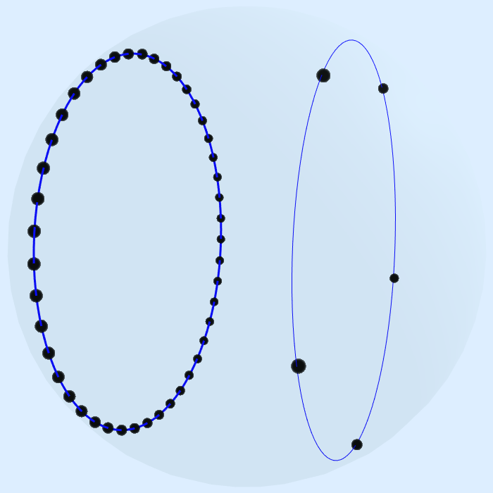
Figure 3.1. The target measure $\mu$ is supported on two circles on the sphere $\mathbb{S}^{2}$ with weight ratio $9/1$. Numerical minimization of (3.9) splits $50$ points into $45$ points equally distributed on one and $5$ points on the other circle.

4. Discrepancy kernels on compact sets

Here we discuss discrepancy kernels that extend the kernels of the previous section in a natural way. For $d\geq 1$, let us define the half-space

$$\Omega^{d}_{r}(z):=\{x\in\mathbb{R}^{d}:\langle z,x\rangle\geq r\}\in\mathscr{B}(\mathbb{R}^{d}),\quad z\in\mathbb{S}^{d-1},\quad r\in\mathbb{R}.$$

For fixed $s>0$, we consider the mapping $h:[-s,s]\times\mathbb{S}^{d-1}\rightarrow\mathscr{B}(\mathbb{R}^{d})$ defined by $(r,z)\mapsto\Omega^{d}_{r}(z)$ and endow $[-s,s]$ with the Lebesgue measure ${\mathrm{d}}r$. The push-forward measure $\beta_{d,s}:=h_{*}({\mathrm{d}}r\otimes\sigma_{\mathbb{S}^{d-1}})$ leads to the associated $L_{2}$-discrepancy

$$\mathscr{D}_{\beta_{d,s}}(\mu,\nu_{n})=\int_{-s}^{s}\int_{\mathbb{S}^{d-1}}\left|\mu(\Omega^{d}_{r}(z))-\nu_{n}(\Omega^{d}_{r}(z))\right|^{2}{\rm d}\sigma_{\mathbb{S}^{d-1}}(z){\rm d}r.$$

The associated discrepancy kernel is

(4.1) $$K_{\beta_{d,s}}(x,y)=\int_{-s}^{s}\int_{\mathbb{S}^{d-1}}\delta_{x}(\Omega^{d}_{r}(z))\delta_{y}(\Omega^{d}_{r}(z)){\rm d}\sigma_{\mathbb{S}^{d-1}}(z){\rm d}r,\qquad x,y\in\mathbb{R}^{d}.$$

Since $B^{\mathbb{S}^{d-1}}_{r}(z)=\Omega^{d}_{\cos(r)}(z)\cap\mathbb{S}^{d-1}$, for $r\in[0,\pi]$ and $z\in\mathbb{S}^{d-1}$, we deduce

$$K_{\beta_{d}}|_{\mathbb{S}^{d-1}\times\mathbb{S}^{d-1}}=K_{\beta_{d,1}}|_{\mathbb{S}^{d-1}\times\mathbb{S}^{d-1}},\qquad d\geq 2,$$

with $K_{\beta_{d}}$ as in (3.1). In contrast to $K_{\beta_{d}}$, the kernel $K_{\beta_{d,s}}$ is not identically zero outside of $\mathbb{S}^{d-1}\times\mathbb{S}^{d-1}$ and makes also sense for $d=1$.

Example 4.1.

For $d=1$, we have $\mathbb{S}^{0}=\{\pm 1\}$, so that the half-spaces are $\Omega^{1}_{r}(1)=[r,\infty)$ and $\Omega^{1}_{r}(-1)=(-\infty,-r]$. Direct calculation of (4.1) yields

$$K_{\beta_{1,s}}(x,y)=\begin{cases}s-\frac{1}{2}|x-y|,&|x|,|y|\leq s,\\ \frac{s}{2}+\frac{xy}{2|y|},&|x|\leq s\leq|y|,\\ s\operatorname*{H}(xy),&s\leq|x|,|y|,\end{cases}$$

where $\operatorname*{H}$ is the Heaviside step function.

Proposition 4.2.

The Fourier expansion of the kernel $K_{\beta_{1,s}}|_{[-s,s]\times[-s,s]}$ with respect to the Lebesgue measure $\sigma_{[-s,s]}$ on $[-s,s]$ is

$$K_{\beta_{1,s}}(x,y)=\sum_{\begin{subarray}{c}m\in\mathbb{N}\\ m\text{ odd}\end{subarray}}\frac{4}{m^{2}\pi^{2}}\cdot\frac{1}{s}\cdot\sin(\frac{\pi}{2s}mx)\sin(\frac{\pi}{2s}my)\\ +\sum_{\{u>0\,:\,\tan(u)=\frac{1}{u}\}}\frac{1}{u^{2}}\cdot\frac{1}{s(\sin(u)^{2}+1)}\cdot\cos(\frac{u}{s}x)\cos(\frac{u}{s}y),\quad x,y\in[-s,s].$$

Its reproducing kernel Hilbert space is

$$\mathscr{H}_{K_{\beta_{1,s}}}([-s,s])=\{f:[-s,s]\rightarrow\mathbb{C}\;:\;f\text{ is absolutely continuous, }f^{\prime}\in L_{2}([-s,s])\},$$

where the inner product between $f$ and $g$ is given by

$$\frac{1}{2s}\big{(}f(-s)+f(s)\big{)}\big{(}\overline{g(-s)+g(s)}\big{)}+\langle f^{\prime},g^{\prime}\rangle_{L_{2}([-s,s])}.$$

Note that $\mathscr{H}_{K_{\beta_{1,s}}}([-s,s])$ is continuously embedded into $\mathbb{H}^{1}([-s,s])$. The proof of Proposition 4.2 is presented in Appendix C. It uses that, up to a constant, $K_{\beta_{1,s}}|_{[-s,s]\times[-s,s]}$ is the Green’s function of the $1$-dimensional harmonic equation $\Delta u=f$ on $[-s,s]$ with the boundary conditions $u^{\prime}(s)=-u^{\prime}(-s)$ and $u(s)+u(-s)=-2u^{\prime}(s)$.

It turns out that $K_{\beta_{d,s}}$ has a simple form on $\mathbb{B}^{d}_{s}\times\mathbb{B}^{d}_{s}$.

Theorem 4.3.

For $d\geq 1$, the discrepancy kernel $K_{\beta_{d,s}}$ satisfies

(4.2) $$K_{\beta_{d,s}}(x,y)=s-\frac{\Gamma(\frac{d}{2})}{2\sqrt{\pi}\Gamma(\frac{d+1}{2})}\|x-y\|,\qquad x,y\in\mathbb{B}^{d}_{s}.$$

The identity (4.2) for $x,y\in\mathbb{S}^{d-1}$ with $s=1$ has been established in [13], see also (3.2). Essentially, the same proof still works for the more general situation. Theorem 4.3 provides a simple form of $K_{\beta_{d,s}}|_{\mathbb{X}\times\mathbb{X}}$ with $\mathbb{X}=\mathbb{B}^{d}_{s}$, which may facilitate further computations. An immediate consequence is $\mathscr{D}_{\beta_{d,s}}(\delta_{x},\delta_{y})=\frac{\Gamma(\frac{d}{2})}{\sqrt{\pi}\Gamma(\frac{d+1}{2})}\|x-y\|$, for $x,y\in\mathbb{B}^{d}_{s}$.

5. The Euclidean ball $\mathbb{B}^{d}$

This section is dedicated to derive the Fourier expansion of the discrepancy kernel $K_{\beta_{d,1}}$ in (4.1) on $\mathbb{B}^{d}$. Proposition 4.2 has covered $d=1$, and we now derive the spectral decomposition of

$$K^{d,p}:\mathbb{B}^{d}\times\mathbb{B}^{d}\rightarrow\mathbb{R},\qquad(x,y)\mapsto\|x-y\|^{p},$$

for all odd $d$ with odd $p>1-d$ with respect to the Lebesgue measure $\sigma_{\mathbb{B}^{d}}$ on $\mathbb{B}^{d}$. The case $d=3$ with $p=-1$ is discussed in [37].

Let $\{\mathcal{C}^{\alpha}_{m}:m\in\mathbb{N},\;\alpha>-1/2\}$ denote the family of Gegenbauer polynomials with the standard normalization

$$\mathcal{C}^{\alpha}_{m}(1)=\binom{m+2\alpha-1}{m}=\frac{\Gamma(m+2\alpha)}{\Gamma(2\alpha)\Gamma(m+1)},\quad\alpha\neq 0.$$

By $\alpha=\frac{d}{2}-1$, the addition theorem for spherical harmonics yields

(5.1) $$\sum_{l=1}^{Z(d,m)}Y^{m}_{l}(x)\overline{Y^{m}_{l}(y)}=\tfrac{2m+d-2}{d-2}\mathcal{C}^{\frac{d}{2}-1}_{m}(\langle x,y\rangle),\quad x,y\in\mathbb{S}^{d-1}.$$

For $m\in\mathbb{N}$, let us define the kernels $\mathcal{K}^{d,p}_{m}:[0,1]\times[0,1]\rightarrow\mathbb{R}$,

(5.2) $$\mathcal{K}_{m}^{d,p}(r,s)=\!\frac{(-\frac{p}{2})_{m}}{(\frac{d}{2}-1)_{m}}\left(\tfrac{\min(r,s)}{\max(r,s)}\right)^{m}\!\!\max(r,s)^{p}{}_{2}F_{1}{\left(\genfrac{.}{.}{0.0pt}{}{m-\frac{p}{2},1-\frac{d+p}{2}}{m+\frac{d}{2}};\left(\tfrac{\min(r,s)}{\max(r,s)}\right)^{2}\right)}.$$

For $d\geq 3$ and arbitrary real $p>1-d$, we deduce from [18] that

(5.3) $$\|x-y\|^{p}=\sum_{m=0}^{\infty}\mathcal{K}^{d,p}_{m}(\|x\|,\|y\|)\,\mathcal{C}^{\frac{d}{2}-1}_{m}\big{(}\big{\langle}\tfrac{x}{\|x\|},\tfrac{y}{\|y\|}\big{\rangle}\big{)},\quad x,y\in\mathbb{B}^{d},\;(x\neq y\text{ if }p<0).$$

For $x=0$ or $y=0$, the right-hand side of (5.3) is well-defined by analytic continuation.

Using the addition formula (5.1) we obtain

$$K^{d,p}(x,y)=\sum_{m=0}^{\infty}\tfrac{d-2}{2m+d-2}\mathcal{K}^{d,p}_{m}(\|x\|,\|y\|)\sum_{l=1}^{Z(d,m)}Y^{m}_{l}(\tfrac{x}{\|x\|})Y^{m}_{l}(\tfrac{y}{\|y\|}),\quad x,y\in\mathbb{B}^{d}.$$

The Fourier expansion of $\mathcal{K}_{m}^{d,p}$ with respect to the measure $r^{d-1}\mathrm{d}r$ satisfies

(5.4) $$\mathcal{K}_{m}^{d,p}(r,s)=\sum_{j=1}^{\infty}\lambda_{m,j}^{d,p}\varphi_{m,j}^{d,p}(r)\varphi_{m,j}^{d,p}(s),\qquad\int_{0}^{1}\mathcal{K}_{m}^{d,p}(r,s)\varphi_{m,j}^{d,p}(r)r^{d-1}\mathrm{d}r=\lambda_{m,j}^{d,p}\varphi^{d,p}_{m,j}(s),$$

where $\int_{0}^{1}|\varphi_{m,j}^{d,p}(r)|^{2}r^{d-1}\mathrm{d}r=1$. Then, by setting

$$\varphi_{m^{\prime},j^{\prime},l^{\prime}}^{d,p}(x):=\varphi_{m^{\prime},j^{\prime}}^{d,p}(\|x\|)Y^{m^{\prime}}_{l^{\prime}}(\tfrac{x}{\|x\|}),\quad x\in\mathbb{B}^{d},$$

direct computations yield

(5.5) $$T^{d,p}\varphi_{m^{\prime},j^{\prime},l^{\prime}}^{d,p}(x)=\lambda_{m^{\prime},j^{\prime}}^{d,p}\tfrac{(d-2)\mathrm{vol}(\mathbb{S}^{d-1})}{2m^{\prime}+d-2}\varphi_{m^{\prime},j^{\prime},l^{\prime}}^{d,p}(x)$$

with the scaling $\int_{\mathbb{B}^{d}}\left|\varphi_{m^{\prime},j^{\prime},l^{\prime}}^{d,p}(x)\right|^{2}\mathrm{d}x=\mathrm{vol}(\mathbb{S}^{d-1})$. This leads to the Fourier expansion

(5.6) $$K^{d,p}(x,y) =\sum_{m=0}^{\infty}\sum_{j=1}^{\infty}\lambda_{m,j}^{d,p}\tfrac{(d-2)\mathrm{vol}(\mathbb{S}^{d-1})}{2m+d-2}\sum_{l=1}^{Z(d,m)}\frac{\varphi^{d,p}_{m,j,l}(x)}{\sqrt{\mathrm{vol}(\mathbb{S}^{d-1})}}\frac{\varphi^{d,p}_{m,j,l}(y)}{\sqrt{\mathrm{vol}(\mathbb{S}^{d-1})}},\quad x,y\in\mathbb{B}^{d}.$$

Thus, the original problem is reduced to the spectral decomposition of the sequence of kernels $\mathcal{K}^{d,p}_{m}$, for $m\in\mathbb{N}$. The kernel $\mathcal{K}^{d,p}_{m}$ induces the integral operator

(5.7) $$T_{m}^{d,p}:L_{2}([0,1],r^{d-1}{\rm d}r)\rightarrow\mathcal{C}([0,1]),\quad f\mapsto\int_{0}^{1}\mathcal{K}^{d,p}_{m}(\cdot,r)f(r)r^{d-1}{\rm d}r,$$

with eigenvalues $\lambda^{d,p}_{m,j}$ and eigenfunctions $\varphi^{d,p}_{m,j}$. We now specify these eigenvalues and eigenfunctions, where $J_{\nu}$ denotes the Bessel function of the first kind of order $\nu$ and $\zeta_{k}:={\rm e}^{2\pi{\rm i}/k}$ is the $k$-th root of unity.

Theorem 5.1.

Suppose that both $d\geq 3$ and $p>1-d$ are odd and let $m\in\mathbb{N}$. Then the following holds:

• Any eigenvalue $\lambda\neq 0$ of $T_{m}^{d,p}$ is in a one-to-one correspondence with

  (5.8) $$\omega=\big{|}\lambda^{-1}2^{d+p-2}(d+2m-2)(-\tfrac{p}{2})_{\frac{d+p}{2}-1}(\tfrac{d+p}{2}-1)!\big{|}^{\frac{1}{d+p}}$$

  with $\omega$ satisfying $\det(A(\omega))=0$, where

  (5.9) $$A(\omega)=\begin{cases}\left(\zeta_{d+p}^{-i\ell}J_{m+\frac{d}{2}-i-1}(\zeta_{d+p}^{\ell}\omega)\right)_{i=1,\,\ell=0}^{\frac{d+p}{2},\,\frac{d+p}{2}-1},&(-\tfrac{p}{2})_{\frac{d+p}{2}-1}\lambda>0,\\ \left(\zeta_{2(d+p)}^{-i(2\ell+1)}J_{m+\frac{d}{2}-i-1}(\zeta_{2(d+p)}^{2\ell+1}\omega)\right)_{i=1,\,\ell=0}^{\frac{d+p}{2},\,\frac{d+p}{2}-1},&(-\tfrac{p}{2})_{\frac{d+p}{2}-1}\lambda<0.\\ \end{cases}$$

• The eigenfunctions are exactly

  $$r\mapsto\begin{cases}\sum_{\ell=1}^{\frac{d+p}{2}}c_{\ell}\,r^{1-\frac{d}{2}}J_{m+\frac{d}{2}-1}(\zeta^{\ell-1}_{d+p}\omega r),&(-\tfrac{p}{2})_{\frac{d+p}{2}-1}\lambda>0,\\ \sum_{\ell=1}^{\frac{d+p}{2}}c_{\ell}\,r^{1-\frac{d}{2}}J_{m+\frac{d}{2}-1}(\zeta^{2\ell-1}_{2(d+p)}\omega r),&(-\tfrac{p}{2})_{\frac{d+p}{2}-1}\lambda<0,\\ \end{cases}$$

  where $c\in\mathbb{R}^{\frac{d+p}{2}}$ is in the nullspace of $A(\omega)$.

Remark 5.2.

Computer experiments seem to indicate that the nullspace of $A(\omega)$ is one-dimensional if $\det(A(\omega))=0$. In that case, the function

(5.10) $$r\mapsto\begin{cases}\sum_{\ell=1}^{\frac{d+p}{2}}(-1)^{\ell}A_{[1,\ell]}(\omega)\,r^{1-\frac{d}{2}}J_{m+\frac{d}{2}-1}(\zeta^{\ell-1}_{d+p}\omega r),&(-\tfrac{p}{2})_{\frac{d+p}{2}-1}\lambda>0,\\ \sum_{\ell=1}^{\frac{d+p}{2}}(-1)^{\ell}A_{[1,\ell]}(\omega)\,r^{1-\frac{d}{2}}J_{m+\frac{d}{2}-1}(\zeta^{2\ell-1}_{2(d+p)}\omega r),&(-\tfrac{p}{2})_{\frac{d+p}{2}-1}\lambda<0,\end{cases}$$

where $A_{[1,\ell]}(\omega)$ denotes the $(1,\ell)$ minor of $A(\omega)$, spans the eigenspace associated with $\lambda$.

Appendix D is dedicated to the proof of Theorem 5.1. The proof reveals strong ties with polyharmonic operators on the unit ball and higher order differential operators on the interval $[0,1]$. We refer to [1] for structurally related spectral decompositions of polyharmonic operators on $[0,1]$ with homogeneous Neumann boundary conditions.

Corollary 5.3 ($d=3$, $p=1$).

The nonzero eigenvalues of $T^{3,1}_{m}$ for $m\in\mathbb{N}\setminus\{0\}$ are exactly the positive solutions of the equation

$$J_{m-\frac{1}{2}}(\omega)J_{m-\frac{3}{2}}(\mathrm{i}\omega)-\mathrm{i}J_{m-\frac{1}{2}}(\mathrm{i}\omega)J_{m-\frac{3}{2}}(\omega)=0,$$

with $\lambda=-\omega^{-4}(4m+2)$. The corresponding eigenspaces are $1$-dimensional with the representative

(5.11) $$f_{\lambda}(r)=r^{-\frac{1}{2}}\left(J_{m+\frac{1}{2}}(\omega r)\mathrm{i}J_{m-\frac{1}{2}}(\mathrm{i}\omega)+J_{m+\frac{1}{2}}(\mathrm{i}\omega r)J_{m-\frac{1}{2}}(\omega)\right).$$

The formulas in Corollary 5.3 are derived from Theorem 5.1. Since $J_{m-\frac{1}{2}}({\rm i}\omega)\neq 0$, for all $\omega\in\mathbb{R}\setminus\{0\}$, the eigenspaces are $1$-dimensional and (5.11) is not the zero-function.

In view of (4.2) in Theorem 4.3 we are particularly interested in kernels of the form $c-\|x-y\|$. In this case, the expansion holds with $-\mathcal{K}^{d,1}_{m}$ for $m\geq 1$ and $c-\mathcal{K}^{d,1}_{0}$ for $m=0$.

6. The rotation group $\operatorname*{SO}(3)$

In this section we derive the Fourier expansion of the discrepancy kernel on the special orthogonal group $\operatorname*{SO}(3)$. The eigenfunctions turn out to be classical functions but the coefficients and their decay rates need to be determined. We also provide numerical experiments by using the nonequispaced fast Fourier transform on $\operatorname*{SO}(3)$.

6.1. Fourier expansion on $\operatorname*{SO}(3)$

By identifying $\mathbb{R}^{d\times d}$ with $\mathbb{R}^{d^{2}}$, Theorem 4.3 applies to subsets of $\mathbb{R}^{d\times d}$ endowed with the trace inner product

$$\langle x,y\rangle_{\operatorname{F}}:=\operatorname*{trace}(x^{\top}y),\quad x,y\in\mathbb{R}^{d\times d},$$

and the induced Frobenius norm $\|\cdot\|_{\operatorname{F}}$ on $\mathbb{R}^{d\times d}$. In this way, $\operatorname*{SO}(3)$ is contained in $\mathbb{B}^{9}_{\sqrt{3}}$, and it is natural to consider ${s}=\sqrt{3}$. We endow $\operatorname*{SO}(3)$ with the normalized Haar measure $\sigma_{\operatorname*{SO}(3)}$. Let $\{\mathcal{D}^{m}_{k,l}:k,l=-m,\ldots,m\}$ denote the Wigner $\mathcal{D}$-functions on $\operatorname*{SO}(3)$, which are closely related to the irreducible representations of $\operatorname*{SO}(3)$ and provide an orthonormal basis for $L_{2}(\operatorname*{SO}(3))$, cf. [48]. For $p>0$, the Fourier expansion

(6.1) $$2^{-\frac{p}{2}}\|x-y\|^{p}_{\operatorname{F}}=\sum_{m=0}^{\infty}a_{m}(p,\operatorname*{SO}(3))\sum_{k,l=-m}^{m}\mathcal{D}^{m}_{k,l}(x)\overline{\mathcal{D}^{m}_{k,l}(y)},\quad x,y\in\operatorname*{SO}(3),$$

holds and, analogous to (3.5), the coefficients are determined by

(6.2) $$a_{m}(p,\operatorname*{SO}(3)):=\iint\limits_{\operatorname*{SO}(3)\times\operatorname*{SO}(3)}2^{-\frac{p}{2}}\|x-y\|_{\operatorname{F}}^{p}\overline{\mathcal{D}^{m}_{k,l}(x)}\mathcal{D}^{m}_{k,l}(y){\rm d}\sigma_{\operatorname*{SO}(3)}(x){\rm d}\sigma_{\operatorname*{SO}(3)}(y).$$

We now compute these coefficients for the entire range $p>-3$.

Proposition 6.1.

For $p>-3$, the coefficients (6.2) are

(6.3) $$a_{m}(p,\operatorname*{SO}(3))=\frac{2^{p}\Gamma(\frac{p}{2}+\frac{3}{2})}{\sqrt{\pi}\Gamma(-\frac{p}{2})}\cdot\frac{\Gamma(-\frac{p}{2}+m)}{\Gamma(\frac{p}{2}+2+m)}\cdot\frac{1}{(m+\frac{1}{2})}.$$

In particular, if $p\not\in 2\mathbb{N}$, then

$$|a_{m}(p,\operatorname*{SO}(3))|=\left|\frac{2^{p}\Gamma(\frac{p}{2}+\frac{3}{2})}{\sqrt{\pi}\Gamma(-\frac{p}{2})}\right|m^{-(p+3)}(1+o(1)),\qquad m\in\mathbb{N},$$

and the series (6.1) terminates if $p\in 2\mathbb{N}$.

The proof is given in Appendix E. For $p\in 2\mathbb{N}$, we again apply the convention $\frac{\Gamma(-\frac{p}{2}+m)}{\Gamma(-\frac{p}{2})}=(-\frac{p}{2})_{m}$ in (6.3), so that $a_{m}(p,\operatorname*{SO}(3))=0$ for all $m>\frac{p}{2}$ if $p\in 2\mathbb{N}$. Provided that $\tau>3/2$, the Sobolev space $\mathbb{H}^{\tau}(\operatorname*{SO}(3))$ is the reproducing kernel Hilbert space associated with the reproducing kernel

$$(x,y)\mapsto\sum_{m=0}^{\infty}(1+m(m+1))^{-\tau}\sum_{k,l=-m}^{m}\mathcal{D}^{m}_{k,l}(x)\overline{\mathcal{D}^{m}_{k,l}(y)},\quad x,y\in\operatorname*{SO}(3).$$

The choice $p=1$ in Proposition 6.1 implies that the kernel $K_{\beta_{9,s}}|_{\operatorname*{SO}(3)\times\operatorname*{SO}(3)}$ reproduces the Sobolev space $\mathscr{H}_{K_{\beta_{9,s}}}(\operatorname*{SO}(3))=\mathbb{H}^{2}(\operatorname*{SO}(3))$ with an equivalent norm provided that $s\geq\sqrt{3}$.

For $d\geq 2$, $K_{\beta_{d^{2},\sqrt{d}}}|_{\operatorname*{SO}(d)\times\operatorname*{SO}(d)}$ reproduces the Sobolev space $\mathbb{H}^{\frac{d(d-1)+2}{4}}(\operatorname*{SO}(d))$ with an equivalent norm. Indeed, Theorem 4.3 and Section 3 yield that $K_{\beta_{d^{2},d}}|_{\mathbb{S}^{d^{2}-1}\times\mathbb{S}^{d^{2}-1}}$ reproduces $\mathbb{H}^{\frac{d^{2}}{2}}(\mathbb{S}^{d^{2}-1})$ with equivalent norms. Rescaling implies that $K_{\beta_{d^{2},d}}|_{d\,\mathbb{S}^{d^{2}-1}\times d\,\mathbb{S}^{d^{2}-1}}$ reproduces $\mathbb{H}^{\frac{d^{2}}{2}}({d\,}\mathbb{S}^{d^{2}-1})$. Since $\operatorname*{SO}(d)\subset d\,\mathbb{S}^{d^{2}-1}$, the assertion for $\operatorname*{SO}(d)$ follows from results on restricting kernels in [26].

6.2. Numerical examples on $\operatorname*{SO}(3)$

Proposition 6.1 yields the coefficients of the kernel expansion

$$K_{\beta_{9,\sqrt{3}}}(x,y)=\sum_{m=0}^{\infty}a_{m}\sum_{k,l=-m}^{m}\mathcal{D}^{m}_{k,l}(x)\overline{\mathcal{D}^{m}_{k,l}(y)},\quad x,y\in\operatorname*{SO}(3).$$

For $\textnormal{supp}(\mu),\textnormal{supp}(\nu_{n})\subset\operatorname*{SO}(3)$, the $L_{2}$-discrepancy (1.6) for $K_{\beta_{9,\sqrt{3}}}$ becomes

(6.4) $$\mathscr{D}_{\beta_{9,\sqrt{3}}}(\mu,\nu_{n})=\sum_{m=0}^{\infty}a_{m}\sum_{k,l=-m}^{m}\left|\hat{\mu}^{m}_{k,l}-\frac{1}{n}\sum_{j=1}^{n}\overline{\mathcal{D}^{m}_{k,l}(x_{j})}\right|^{2},$$

where $\hat{\mu}^{m}_{k,l}$ denotes the Fourier coefficient of $\mu$ with respect to $\mathcal{D}^{m}_{k,l}$, cf. (1.6). We truncate the series (6.4) at $M=8$ and minimize

(6.5) $$\sum_{m=0}^{M}a_{m}\sum_{k,l=-m}^{m}\left|\hat{\mu}^{m}_{k,l}-\frac{1}{n}\sum_{j=1}^{n}\overline{\mathcal{D}^{m}_{k,l}(x_{j})}\right|^{2}$$

among all $n$-point sets $\{x_{1},\ldots,x_{n}\}\subset\operatorname*{SO}(3)$ for fixed $n=30$. We efficiently solve the least squares minimization by using the nonequispaced fast Fourier transform on $\operatorname*{SO}(3)$, cf. [32, 44]. Figure 6.1 shows the minimizing points mapped onto $\mathbb{B}^{3}$.

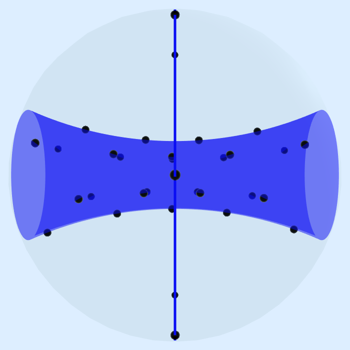
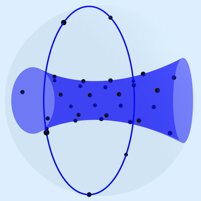
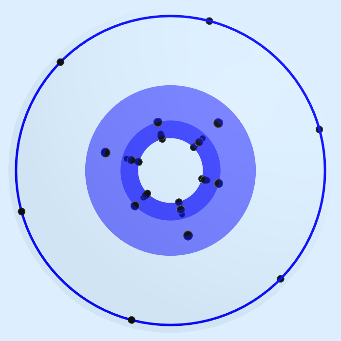
Figure 6.1. We use the standard parametrization of $\operatorname*{SO}(3)$ by $\mathbb{S}^{3}$ via unit quaternions, which is then mapped into $\mathbb{B}^{3}$ by stereographic projection. The target measure $\mu$ is supported on two disjoint parts with weight ratio $9/1$ colored in darker blue by the cylindrical surface and the great circle. Numerical minimization of (6.5) splits $30$ points in $\operatorname*{SO}(3)$ into $27$ points on the inner surface and $3$ points on the great circle. We plotted $6$ points on the great circle but antipodal points correspond to the same point in $\operatorname*{SO}(3)$.

7. The Grassmannian $\operatorname{\mathcal{G}}_{2,4}$

First, the Fourier expansion of the discrepancy kernel on $\operatorname{\mathcal{G}}_{2,4}$ is computed. To prepare for developing the nonequispaced fast Fourier transform on $\operatorname{\mathcal{G}}_{2,4}$, we then explicitly parametrize the Grassmannian $\operatorname{\mathcal{G}}_{2,4}$ by its double covering $\mathbb{S}^{2}\times\mathbb{S}^{2}$. Next, we derive the nonequispaced fast Fourier transform on $\mathbb{S}^{2}\times\mathbb{S}^{2}$ and provide numerical minimization experiments on $\operatorname{\mathcal{G}}_{2,4}$.

7.1. Fourier expansion on $\operatorname{\mathcal{G}}_{2,4}$

Proposition 4.3 also applies to the Grassmannian

$$\operatorname{\mathcal{G}}_{2,4}:=\{x\in\mathbb{R}^{4\times 4}:x^{\top}=x,\;x^{2}=x,\;\operatorname{rank}(x)=2\}$$

with $s=\sqrt{2}$ when $\mathbb{R}^{4\times 4}$ is identified with $\mathbb{R}^{16}$. To derive the Fourier expansion on $\operatorname{\mathcal{G}}_{2,4}$, we require some preparations. We shall use integer partitions $\lambda=(\lambda_{1},\lambda_{2})\in\mathbb{N}^{2}$ with $\lambda_{1}\geq\lambda_{2}\geq 0$. We also denote $|\lambda|:=\lambda_{1}+\lambda_{2}$. The orthogonal group $\operatorname{O}(4)$ acts transitively on $\operatorname{\mathcal{G}}_{2,4}$ by conjugation and induces the irreducible decomposition

(7.1) $$L_{2}(\operatorname{\mathcal{G}}_{2,4},\sigma_{\operatorname{\mathcal{G}}_{2,4}})=\bigoplus_{\lambda_{1}\geq\lambda_{2}\geq 0}H_{\lambda}(\operatorname{\mathcal{G}}_{2,4}),\qquad H_{\lambda}(\operatorname{\mathcal{G}}_{2,4})\perp H_{\lambda^{\prime}}(\operatorname{\mathcal{G}}_{2,4}),\quad\lambda\neq\lambda^{\prime},$$

where $\sigma_{\operatorname{\mathcal{G}}_{2,4}}$ is the normalized orthogonally invariant measure on $\operatorname{\mathcal{G}}_{2,4}$ and $H_{\lambda}(\operatorname{\mathcal{G}}_{2,4})$ is equivalent to the irreducible representation $\mathcal{H}_{2\lambda}^{4}$ of $\operatorname{O}(4)$ with type $2\lambda$, cf. [8, 35]. The normalized eigenfunctions of the Laplace–Beltrami operator on $\operatorname{\mathcal{G}}_{2,4}$ form an orthonormal basis for $L_{2}(\operatorname{\mathcal{G}}_{2,4})$, and each $H_{\lambda}(\operatorname{\mathcal{G}}_{k,d})$ is contained in the eigenspace $E_{\alpha_{\lambda}}$ associated with the eigenvalue $\alpha_{\lambda}=4(\lambda_{1}^{2}+\lambda_{2}^{2}+\lambda_{1})$, cf. [6, 7, 8, 23, 35, 45].

Let $Q_{\lambda}$ be the reproducing kernel of $H_{\lambda}(\operatorname{\mathcal{G}}_{2,4})$. Any orthonormal basis $\{\varphi_{\lambda,l}\}_{l=1}^{\dim(\mathcal{H}^{4}_{2\lambda})}$ for $H_{\lambda}(\operatorname{\mathcal{G}}_{2,4})$ yields the spectral decomposition

(7.2) $$Q_{\lambda}(x,y)=\sum_{l=1}^{\dim(\mathcal{H}^{4}_{2\lambda})}\varphi_{\lambda,l}(x)\overline{\varphi_{\lambda,l}(y)},\qquad x,y\in\operatorname{\mathcal{G}}_{2,4},\quad\lambda_{1}\geq\lambda_{2}\geq 0.$$

The orthogonal decomposition (7.1) leads to the Fourier expansion

(7.3) $$2^{-\frac{p}{2}}\|x-y\|_{\operatorname{F}}^{p}=\sum_{\lambda_{1}\geq\lambda_{2}\geq 0}a_{\lambda}(p,\operatorname{\mathcal{G}}_{2,4})Q_{\lambda}(x,y),\qquad x,y\in\operatorname{\mathcal{G}}_{2,4},\quad p>0.$$

The coefficients $a_{\lambda}(p,\operatorname{\mathcal{G}}_{2,4})$ in (7.3) are defined by

(7.4) $$a_{\lambda}(p,\operatorname{\mathcal{G}}_{2,4}):=\frac{1}{\dim(\mathcal{H}^{4}_{2\lambda})}\iint\limits_{\operatorname{\mathcal{G}}_{2,4}\times\operatorname{\mathcal{G}}_{2,4}}2^{-\frac{p}{2}}\|x-y\|_{\operatorname{F}}^{p}Q_{\lambda}(x,y){\rm d}\sigma_{\operatorname{\mathcal{G}}_{2,4}}(x){\rm d}\sigma_{\operatorname{\mathcal{G}}_{2,4}}(y).$$

In order to determine $a_{\lambda}(p,\operatorname{\mathcal{G}}_{2,4})$, we shall make use of the hypergeometric coefficients $(f)_{(\lambda_{1},\lambda_{2})}:=(f)_{\lambda_{1}}(f-\tfrac{1}{2})_{\lambda_{2}}$.

Theorem 7.1.

For $p>-4$, we have

(7.5) $$a_{\lambda}(p,\operatorname{\mathcal{G}}_{2,4})=\frac{4^{-|\lambda|}|\lambda|!}{(\tfrac{3}{2})_{|\lambda|}(\tfrac{3}{2})_{\lambda}}(-\tfrac{p}{2})_{|\lambda|}\;{}_{4}F_{3}{\left(\genfrac{.}{.}{0.0pt}{}{\tfrac{|\lambda|+1}{2},\tfrac{|\lambda|+2}{2},\tfrac{|\lambda|}{2}-\tfrac{p}{4},\tfrac{|\lambda|+1}{2}-\tfrac{p}{4}}{|\lambda|+\tfrac{3}{2},\lambda_{1}+\tfrac{3}{2},\lambda_{2}+1};1\right)}.$$

In particular, if $p\not\in 2\mathbb{N}$, then

(7.6) $$|a_{\lambda}(p,\operatorname{\mathcal{G}}_{2,4})|=\left|\frac{\Gamma(\frac{p}{2}+2)}{2\Gamma(-\frac{p}{2})}\right|\|\lambda\|^{-(p+4)}(1+o(1)),\qquad\lambda_{1}\geq\lambda_{2}\geq 0,$$

and the series (7.3) terminates if $p\in 2\mathbb{N}$.

The proof of this theorem is contained in Section F.1 of Appendix F. If $p\in 2\mathbb{N}$, then $a_{\lambda}(p,\operatorname{\mathcal{G}}_{2,4})=0$ for all $|\lambda|>\frac{p}{2}$. For $\tau>2$, the Sobolev space $\mathbb{H}^{\tau}(\operatorname{\mathcal{G}}_{2,4})$ is the reproducing kernel Hilbert space with associated reproducing kernel

(7.7) $$(x,y)\mapsto\sum_{\lambda_{1}\geq\lambda_{2}\geq 0}(1+4\lambda_{1}^{2}+4\lambda_{2}^{2}+4\lambda_{1})^{-\tau}Q_{\lambda}(x,y),\quad x,y\in\operatorname{\mathcal{G}}_{2,4},$$

cf. [11, 16]. Since the coefficients in (7.7) behave asymptotically as $\|\lambda\|^{-2\tau}$, the choice $p=1$ in Theorem 7.1 implies that the kernel $K_{\beta_{16,s}}|_{\operatorname{\mathcal{G}}_{2,4}\times\operatorname{\mathcal{G}}_{2,4}}$ reproduces the Sobolev space $\mathscr{H}_{K_{\beta_{16,s}}}(\operatorname{\mathcal{G}}_{2,4})=\mathbb{H}^{\frac{5}{2}}(\operatorname{\mathcal{G}}_{2,4})$ with an equivalent norm provided that $s\geq\sqrt{2}$.

By invoking [26], we deduce that, for $d\geq 2$, $K_{\beta_{d^{2},\sqrt{k}}}|_{\operatorname{\mathcal{G}}_{k,d}\times\operatorname{\mathcal{G}}_{k,d}}$ reproduces the Sobolev space $\mathbb{H}^{\frac{k(d-k)+1}{2}}(\operatorname{\mathcal{G}}_{k,d})$ with an equivalent norm.

7.2. Parametrization of $\operatorname{\mathcal{G}}_{2,4}$ by $\faktor{(\mathbb{S}^{2}\times\mathbb{S}^{2})}{\pm 1}$

To derive the nonequispaced fastFourier transform on $\operatorname{\mathcal{G}}_{2,4}$, we shall first explicitly construct the parametrization of $\operatorname{\mathcal{G}}_{2,4}$ by its double covering $\mathbb{S}^{2}\times\mathbb{S}^{2}$. We denote the $d\times d$-identity matrix by $I_{d}$, and the cross-product between two vectors $x,y\in\mathbb{S}^{2}$ is denoted by $x\times y\in\mathbb{R}^{3}$. The mapping $\mathcal{P}:\mathbb{S}^{2}\times\mathbb{S}^{2}\rightarrow\operatorname{\mathcal{G}}_{2,4}$ given by

(7.8) $$(x,y)\mapsto \frac{1}{2}\begin{pmatrix}1+x^{\top}y&&-(x\times y)^{\top}\\ -x\times y&&xy^{\top}+yx^{\top}+(1-x^{\top}y)I_{3}\\ \end{pmatrix}$$

is surjective and, for all $x,y,u,v\in\mathbb{S}^{2}$,

(7.9) $$\mathcal{P}(u,v)=\mathcal{P}(x,y)\quad\text{ if and only if }\quad(u,v)\in\{\pm(x,y)\},$$

see Section F.2 and Theorem F.4 of Appendix F. In order to specify the inverse map, note that $\faktor{\mathbb{S}^{2}\times\mathbb{S}^{2}}{\pm 1}$ can be identified with $\mathcal{M}(3):=\{xy^{\top}\in\mathbb{R}^{3\times 3}:x,y\in\mathbb{S}^{2}\}.$ We now define $\mathcal{L}:\mathcal{G}_{2,4}\rightarrow\mathcal{M}(3)$,

(7.10) $$\mathcal{L}(P):=\left(\begin{smallmatrix}\frac{1}{2}(P_{11}+P_{22}-P_{33}-P_{44})&P_{23}-P_{14}&P_{24}+P_{13}\\ P_{23}+P_{14}&\frac{1}{2}(P_{11}-P_{22}+P_{33}-P_{44})&P_{34}-P_{12}\\ P_{24}-P_{13}&P_{34}+P_{12}&\frac{1}{2}(P_{11}-P_{22}-P_{33}+P_{44})\\ \end{smallmatrix}\right),$$

and direct computations lead to

(7.11) $$\mathcal{L}(\mathcal{P}(x,y))=xy^{\top},\quad x,y\in\mathbb{S}^{2}.$$

The right-hand side determines $x$ and $y$ up to the ambiguity (7.9). Under the Frobenius norm, $\mathcal{P}$ is distance preserving in the sense

(7.12) $$\|\mathcal{P}(x,y)-\mathcal{P}(u,v)\|_{\operatorname{F}}=\|xy^{\top}-uv^{\top}\|_{\operatorname{F}},\quad x,y,u,v\in\mathbb{S}^{2}.$$

The latter follows from (F.20) in Lemma F.6 in Section F.2 of Appendix F.

We shall now check how the spherical harmonics $Y^{m}_{l}$ on $\mathbb{S}^{2}$ relate to the eigenfunctions $\varphi_{\lambda,l}\in H_{\lambda}(\operatorname{\mathcal{G}}_{2,4})$ of the Laplace–Beltrami operator on $\operatorname{\mathcal{G}}_{2,4}$, cf. (7.2). The functions $Y_{k,l}^{m,n}:\mathcal{G}_{2,4}\to\mathbb{C}$ given by

(7.13) $$Y_{k,l}^{m,n}(\mathcal{P}(x,y)):=Y_{k}^{m}(x)\cdot Y_{l}^{n}(y)$$

are well-defined for $m+n\in 2\mathbb{N}$, the latter taking into account the ambiguity (7.9).

Theorem 7.2.

For $m_{\lambda}:=(\lambda_{1}+\lambda_{2})$ and $n_{\lambda}:=(\lambda_{1}-\lambda_{2})$, we have

(7.14) $$H_{\lambda}(\mathcal{G}_{2,4})=\mathrm{span}\{Y_{k,l}^{m_{\lambda},n_{\lambda}},Y_{l,k}^{n_{\lambda},m_{\lambda}}:k=-m_{\lambda},\dots,m_{\lambda},\;l=-n_{\lambda},\dots,n_{\lambda}\}.$$

The proof is presented at the end of Section F.2 of Appendix F. Note that the geodesic distance on $\operatorname{\mathcal{G}}_{2,4}$ is $\operatorname{dist}_{\operatorname{\mathcal{G}}_{2,4}}(P,Q)=\sqrt{2}\sqrt{\theta_{1}^{2}+\theta_{2}^{2}}$, where $\theta_{1},\theta_{2}\in[0,\pi/2]$ are the principal angles determined by the two largest eigenvalues $\cos^{2}(\theta_{1})$ and $\cos^{2}(\theta_{2})$ of the matrix $PQ$. Aside from (7.12), $\mathcal{P}$ is also distance-preserving with respect to the respective geodesic distances, i.e.,

$$\operatorname{dist}_{\operatorname{\mathcal{G}}_{2,4}}(\mathcal{P}(x,y),\mathcal{P}(u,v))=\operatorname{dist}_{\faktor{\mathbb{S}^{2}\times\mathbb{S}^{2}}{\pm 1}}\big{(}\left(\begin{smallmatrix}x\\ y\end{smallmatrix}\right),\left(\begin{smallmatrix}u\\ v\end{smallmatrix}\right)\big{)},\quad x,y,u,v\in\mathbb{S}^{2}.$$

This equality follows from (F.23) in Lemma F.6 in the appendix via further direct calculations.

The identity (7.14) provides explicit expressions for the orthonormal basis $\{\varphi_{\lambda,l}\}_{l=1}^{\dim(\mathcal{H}^{4}_{2\lambda})}$ of $H_{\lambda}(\operatorname{\mathcal{G}}_{2,4})$ that is used to construct the reproducing kernel $Q_{\lambda}$ in (7.2). It also provides a fast Fourier transform on $\operatorname{\mathcal{G}}_{2,4}$ from the respective transform on $\mathbb{S}^{2}\times\mathbb{S}^{2}$ that is developed in the subsequent section.

7.3. Nonequispaced Fast Fourier Transform on $\operatorname{\mathcal{G}}_{2,4}$

The nonequispaced fast (spherical) Fourier transform on $\mathbb{S}^{2}$ has been developed in [39, 41] under the acronym nfsft. Here, we shall derive the analogous transform on $\mathbb{S}^{2}\times\mathbb{S}^{2}$, which induces the nonequispaced fast Fourier transform on $\operatorname{\mathcal{G}}_{2,4}$ via the mapping $\mathcal{P}$ and (7.14) with (7.13).

For a given finite set of coefficients $f^{m_{1},m_{2}}_{k,l}\in\mathbb{C}$, $m_{1},m_{2}=0,\ldots,M$, $k=-m_{1},\ldots,m_{1}$, $l=-m_{2},\ldots,m_{2}$, we aim to evaluate

(7.15) $$F(x,y):=\sum_{m_{1},m_{2}=0}^{M}\sum_{k=-m_{1}}^{m_{1}}\sum_{l=-m_{2}}^{m_{2}}f^{m_{1},m_{2}}_{k,l}Y^{m_{1}}_{k}(x)Y^{m_{2}}_{l}(y)$$

at $n$ scattered locations $(x_{j},y_{j})_{j=1}^{n}\subset\mathbb{S}^{2}\times\mathbb{S}^{2}$. Direct evaluation of (7.15) leads to $O(nM^{4})$ operations. We shall now derive an approximative algorithm that is more efficient for $n\gg M$.

By following the ideas in [39, 41], switching to spherical coordinates reveals that (7.15) is a $4$-dimensional trigonometric polynomial. This enables the use of the $4$-dimensional nonequispaced fast Fourier transform nfft to significantly reduce the complexity. In spherical coordinates the spherical harmonics are trigonometric polynomials such that

(7.16) $$Y^{m}_{k}(z(\theta,\varphi))=e^{{\rm i}k\varphi}\sum_{k^{\prime}=-m}^{m}c^{m}_{k,k^{\prime}}e^{{\rm i}k^{\prime}\theta},\qquad z(\theta,\varphi)=\left(\begin{smallmatrix}\sin(\theta)\cos(\varphi)\\ \sin(\theta)\sin(\varphi)\\ \cos(\theta)\end{smallmatrix}\right)\in\mathbb{S}^{2},$$

where $0\leq\theta\leq\pi$, $0\leq\varphi\leq 2\pi$, and $c^{m}_{k,k^{\prime}}\in\mathbb{C}$ are suitable coefficients that we assume to be given or precomputed. Thus, for $x=z(\theta_{1},\varphi_{1})$ and $y=z(\theta_{2},\varphi_{2})$, there are coefficients $b^{k,l}_{k^{\prime},l^{\prime}}\in\mathbb{C}$ such that

(7.17) $$F(x,y)=\sum_{k,l,k^{\prime},l^{\prime}=-M}^{M}b^{k,l}_{k^{\prime},l^{\prime}}e^{{\rm i}k\varphi_{1}}e^{{\rm i}l\varphi_{2}}e^{{\rm i}k^{\prime}\theta_{1}}e^{{\rm i}l^{\prime}\theta_{2}}.$$

We check in Section F.3 of Appendix F that the set of coefficients $b^{k,l}_{k^{\prime},l^{\prime}}$ can be computed by $O(M^{5})$ operations provided that the numbers $c^{m}_{k,k^{\prime}}$ in (7.16) are given. The expression (7.17) can be evaluated at $n$ scattered locations by the nonequispaced discrete Fourier transform ndft with $O(nM^{4})$ operations, cf. [39, 41]. An efficient approximative algorithm is the nonequispaced fast Fourier transform nfft that requires only $O(M^{4}\log(M)+n|\log(\epsilon)|^{4})$ operations with accuracy $\epsilon$, see [39, 41] for details on accuracy. Thus, our algorithm for evaluating (7.15) at $n$ scattered locations requires $O(M^{5}+n|\log(\epsilon)|^{4})$ operations. For $n\gg M$, this is a significant reduction in complexity compared to the original $O(nM^{4})$ operations. We shall choose $n\sim M^{4}$ in the subsequent section, so that the complexity is reduced from $O(M^{8})$ to $O(M^{5}+M^{4}|\log(\epsilon)|^{4})$ operations. For potential further reduction, we refer to Remark F.7 in the appendix.

7.4. Numerical example on $\operatorname{\mathcal{G}}_{2,4}$

By Theorem 7.1, we can calculate the coefficients of the kernel expansion

$$K_{\beta_{16,\sqrt{2}}}(x,y)=\sum_{\lambda_{1}\geq\lambda_{2}\geq 0}a_{\lambda}\sum_{l=1}^{\dim(\mathcal{H}^{d}_{2\lambda})}\varphi_{\lambda,l}(x)\overline{\varphi_{\lambda,l}(y)},\quad x,y\in\mathcal{G}_{2,4}.$$

The eigenfunctions $\varphi_{\lambda,l}$ are given by the tensor products of spherical harmonics in (7.13), cf. Theorem 7.2. For $\textnormal{supp}(\mu),\textnormal{supp}(\nu_{n})\subset\operatorname{\mathcal{G}}_{2,4}$, the $L_{2}$-discrepancy (1.6) of the kernel $K_{\beta_{16,\sqrt{2}}}|_{\operatorname{\mathcal{G}}_{2,4}\times\operatorname{\mathcal{G}}_{2,4}}$ is

(7.18) $$\mathscr{D}_{\beta_{16,\sqrt{2}}}(\mu,\nu_{n})=\sum_{\lambda_{1}\geq\lambda_{2}\geq 0}a_{\lambda}\sum_{l=1}^{\dim(\mathcal{H}^{d}_{2\lambda})}\left|\hat{\mu}_{\lambda,l}-\frac{1}{n}\sum_{j=1}^{n}\overline{\varphi_{\lambda,l}(x_{j})}\right|^{2},$$

where $\hat{\mu}_{\lambda,l}$ is the Fourier coefficient of $\mu$ with respect to $\varphi_{\lambda,l}$, cf. (1.6).

Let us consider $\mu=\sigma_{\operatorname{\mathcal{G}}_{2,4}}$. According to [11] (see also [15, 16]), the lower bound

$$n^{-5/4}\lesssim\mathscr{D}_{\beta_{16,\sqrt{2}}}(\mu,\nu_{n})$$

holds for all $n$-point sets $\{x_{1},\ldots,x_{n}\}\subset\operatorname{\mathcal{G}}_{2,4}$. We truncate the series (7.18) and let $\nu^{M}_{n}=\frac{1}{n}\sum_{j=1}^{n}\delta_{x^{M}_{j}}$ denote a minimizer of

(7.19) $$\sum_{\lambda+\lambda_{2}\leq M}a_{\lambda}\sum_{l=1}^{\dim(\mathcal{H}^{d}_{2\lambda})}\left|\hat{\mu}_{\lambda,l}-\frac{1}{n}\sum_{j=1}^{n}\overline{\varphi_{\lambda,l}(x_{j})}\right|^{2}$$

among all $n$-point sets $\{x_{1},\ldots,x_{n}\}\subset\operatorname{\mathcal{G}}_{2,4}$. A suitable choice $n\sim M^{4}$ leads to the optimal rate

(7.20) $$\mathscr{D}_{\beta_{16,\sqrt{2}}}(\mu,\nu^{M}_{n})\sim n^{-5/4},$$

cf. [11, 24]. Note that we can efficiently solve the least squares minimization (7.19) by using the nonequispaced fast Fourier transform on $\operatorname{\mathcal{G}}_{2,4}$ derived from the nonequispaced fast Fourier transform on $\mathbb{S}^{2}\times\mathbb{S}^{2}$ of Section 7.3 and applying Theorem  7.2. Figure 7.1 shows logarithmic plots of the number of points versus the $L_{2}$-discrepancy. We observe a line with slope $-5/4$ as predicted by (7.20).

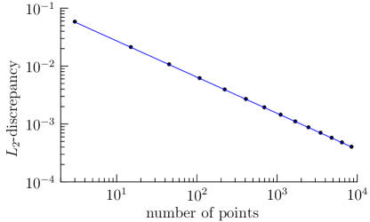
Figure 7.1. Logarithmic plot of the number of points $n$ versus the $L_{2}$-discrepancy $\mathscr{D}_{\beta_{16},\sqrt{2}}(\mu,\nu^{M}_{n})$ on $\operatorname{\mathcal{G}}_{2,4}$, where $\nu^{M}_{n}$ is derived from numerical minimization.

Appendix A Proofs for Section 2

Proof of Theorem 2.1.

Let $h_{d}:[0,\infty)\rightarrow\mathbb{R}$ denote Euclid’s hat function given by

$$h_{d}(\|x\|)=\frac{1}{\operatorname*{vol}(\mathbb{B}^{d}_{1/2})}(1_{\mathbb{B}^{d}_{1/2}}*1_{\mathbb{B}^{d}_{1/2}})(x),\quad x\in\mathbb{R}^{d},$$

where $1_{\mathbb{B}^{d}_{1/2}}$ is the indicator function of $\mathbb{B}^{d}_{1/2}$. For $x,y\in\mathbb{R}^{d}$ and $t=\|x-y\|$, we derive

$$K_{d}(x,y) =\int_{0}^{\infty}\frac{1}{\operatorname*{vol}(\mathbb{B}^{d}_{r/2})}\int_{\mathbb{R}^{d}}1_{\mathbb{B}^{d}_{r/2}(z)}(x)1_{\mathbb{B}^{d}_{r/2}(z)}(y){\rm d}z\,{\rm d}G_{d}(r)=\int_{t}^{\infty}h_{d}(t/r){\rm d}G_{d}(r)$$

$$=\int_{t}^{1}h_{d}(t/r)G_{d}^{\prime}(r){\rm d}r-h_{d}(t)G_{d}(1)=t\int_{t}^{1}r^{-2}h_{d}^{\prime}(t/r)G_{d}(r){\rm d}r,$$

where the last equality is due to partial integration. An explicit expression for $$h^{\prime}_{d}$$ is stated in [28, Equation (11)], so that we obtain

$$K_{d}(x,y) =\frac{d\,\Gamma(\frac{d}{2})}{\sqrt{\pi}\Gamma(\frac{d+1}{2})}t\int_{1}^{\frac{1}{t}}(1-r^{2}t^{2})^{\frac{d-1}{2}}{}_{2}F_{1}{\left(\genfrac{.}{.}{0.0pt}{}{-\frac{d+1}{4},-\frac{d-1}{4}}{-\frac{d}{2}};r^{-2}\right)}{\rm d}r$$

$$=\frac{d\,\Gamma(\frac{d}{2})}{\sqrt{\pi}\Gamma(\frac{d+1}{2})}t\sum_{j=0}^{\frac{d-1}{2}}(-1)^{j}\binom{\frac{d-1}{2}}{j}t^{2j}\sum_{l=0}^{\frac{d+1}{4}}\frac{(-\frac{d+1}{4})_{l}(-\frac{d-1}{4})_{l}}{(-\frac{d}{2})_{l}l!}\int_{1}^{\frac{1}{t}}r^{2(j-l)}{\rm d}r$$

$$=\frac{d\,\Gamma(\frac{d}{2})}{\sqrt{\pi}\Gamma(\frac{d+1}{2})}\sum_{l=0}^{\frac{d+1}{4}}t^{2l}\frac{(-\frac{d+1}{4})_{l}(-\frac{d-1}{4})_{l}}{(-\frac{d}{2})_{l}l!}\sum_{j=0}^{\frac{d-1}{2}}\frac{(-1)^{j}\binom{\frac{d-1}{2}}{j}}{2j-2l+1}$$

$$\qquad\qquad-\frac{d\,\Gamma(\frac{d}{2})}{\sqrt{\pi}\Gamma(\frac{d+1}{2})}\sum_{j=0}^{\frac{d-1}{2}}(-1)^{j}\binom{\frac{d-1}{2}}{j}t^{2j+1}\sum_{l=0}^{\frac{d+1}{4}}\frac{(-\frac{d+1}{4})_{l}(-\frac{d-1}{4})_{l}}{(-\frac{d}{2})_{l}l!(2j-2l+1)}.$$

We now compare coefficients of powers of $t$ with those of the polynomial $(1-t)^{\frac{d+1}{2}}$. In order to check the coefficient of $t^{2l}$, we first observe

$$\sum_{j=0}^{\frac{d-1}{2}}\frac{(-1)^{j}\binom{\frac{d-1}{2}}{j}}{2j-2l+1}={}_{2}F_{1}{\left(\genfrac{.}{.}{0.0pt}{}{-\frac{d-1}{2},\frac{1}{2}-l}{\frac{3}{2}-l};1\right)}\frac{1}{1-2l}=\frac{\Gamma(\frac{d+1}{2})\Gamma(\frac{1}{2}-l)}{2\Gamma(\frac{d}{2}-l+1)},$$

where the last equality makes use of Gauss’ Theorem for the hypergeometric series evaluated at 1 (cf. [47, Equation (1.7.6); Appendix (III.3)]). Direct computation yields

$$\frac{(-\frac{d+1}{4})_{l}(-\frac{d-1}{4})_{l}}{(-\frac{d}{2})_{l}}=\binom{\frac{d+1}{2}}{2l}\frac{(2l)!}{(-4)^{l}}\frac{\Gamma(\frac{d}{2}-l+1)}{\Gamma(\frac{d}{2}+1)},$$

so that the coefficient of $t^{2l}$ in $K_{d}(x,y)$ is

$$\binom{\frac{d+1}{2}}{2l}\frac{(2l)!}{(-4)^{l}l!}\frac{\Gamma(\frac{1}{2}-l)}{\Gamma(\frac{d}{2}+1)2}\frac{d\,\Gamma(\frac{d}{2})}{\sqrt{\pi}}=\binom{\frac{d+1}{2}}{2l}\frac{(2l)!}{(-4)^{l}l!}\frac{\Gamma(\frac{1}{2}-l)}{\sqrt{\pi}}=\binom{\frac{d+1}{2}}{2l}.$$

Hence, the coefficients for even powers of $t$ match. To check the coefficient of $t^{2j+1}$, we first assume $\frac{d-1}{4}\in\mathbb{N}$. The Pfaff–Saalschütz Theorem (cf. [47, Equation (2.3.1.3); Appendix (III.2)]) yields

$$\sum_{l=0}^{\frac{d+1}{4}}\frac{(-\frac{d+1}{4})_{l}(-\frac{d-1}{4})_{l}}{(-\frac{d}{2})_{l}l!(2j-2l+1)} ={}_{3}F_{2}{\left(\genfrac{.}{.}{0.0pt}{}{-\frac{d+1}{4},-\frac{d-1}{4},-\frac{1}{2}-j}{-\frac{d}{2},\frac{1}{2}-j};1\right)}\frac{1}{1+2j}$$

$$=\frac{(-\frac{d-1}{4})_{\frac{d-1}{4}}(j-\frac{d-1}{2})_{\frac{d-1}{4}}}{(-\frac{d}{2})_{\frac{d-1}{4}}(j-\frac{d-3}{4})_{\frac{d-1}{4}}}\frac{1}{1+2j}.$$

Thus, the coefficient of $t^{2j+1}$ in $K_{d}(x,y)$ is nonzero if and only if $j\leq\frac{d-1}{4}$. Moreover, it is given by

$$\frac{-d\,\Gamma(\frac{d}{2})(-1)^{j}\binom{\frac{d-1}{2}}{j}(-\frac{d-1}{4})_{\frac{d-1}{4}}(j-\frac{d-1}{2})_{\frac{d-1}{4}}}{\sqrt{\pi}\Gamma(\frac{d+1}{2})(1+2j)(-\frac{d}{2})_{\frac{d-1}{4}}(j-\frac{d-3}{4})_{\frac{d-1}{4}}}=\frac{-\frac{d}{\sqrt{\pi}}\,\Gamma(\frac{d}{2})(-1)^{j}(\frac{d-1}{4})!(\frac{d+3}{4}-j)_{\frac{d-1}{4}}}{(\frac{d-1}{2}-j)!j!(1+2j)(\frac{d+1}{4}+1)_{\frac{d-1}{4}}(\frac{1}{2}-j)_{\frac{d-1}{4}}}.$$

Further computations using the duplication formula eventually lead to $-\binom{\frac{d+1}{2}}{2l+1}$. The case $\frac{d+1}{4}\in\mathbb{N}$ is checked analogously, and we conclude the proof. ∎

Appendix B Proofs for Section 3

Proof of Proposition 3.2.

By expressing the $\mathbb{R}^{d}$-Fourier transform $\widehat{1_{\mathbb{B}^{d}_{r}}}(\xi)$ in terms of the Bessel function of the first kind of order $d/2$ and using its asymptotics, we deduce

$$\left|\widehat{1_{\mathbb{B}^{d}_{r}}}(\xi)\right|\lesssim\left(1+\|\xi\|^{2}\right)^{-(d+1)/4},\quad\xi\in\mathbb{R}^{d}.$$

Due to the zeros of the Bessel function, the respective lower bound cannot hold. This implies the embedding claims for $\mathbb{H}^{\frac{d+1}{2}}(\mathbb{R}^{d})$, in particular, for $d=3$.

To address the restricted kernel, we observe that the value $K_{d,r}(x,y)$ coincides with the $\mathbb{R}^{d}$-volume of the two intersecting balls $\mathbb{B}^{d}_{r}(x)\cap\mathbb{B}^{d}_{r}(y)$. This volume has been explicitly computed in [31, Section 2.4.3]. For $d=3$, we obtain

$$K_{3,r}(x,y)=\pi(2r-\|x-y\|)^{2}(\|x-y\|+4r)/12,\quad x,y\in\mathbb{S}^{2},$$

so that $K_{3,r}|_{\mathbb{S}^{2}\times\mathbb{S}^{2}}$ is a polynomial of degree $3$ in $\|x-y\|$. Its Fourier coefficients $(a_{m})_{m\in\mathbb{N}}$ are linear combinations of the Fourier coefficients of the monomial terms, so that (3.7) implies $a_{m}\lesssim m^{-3}$.

We have checked that there are no cancelations in these linear combinations. Therefore, the asymptotics (3.7) also imply the associated bound from below, which leads to $a_{m}\sim m^{-3}$. Thus, $K_{3,r}|_{\mathbb{S}^{2}\times\mathbb{S}^{2}}$ reproduces the Sobolev space $\mathbb{H}^{\frac{3}{2}}(\mathbb{S}^{2})$ with equivalent norms. ∎

Appendix C Proofs for Section 4

Proof of Proposition 4.2.

Let us consider $s=1$. The general case follows from rescaling. In order to determine the Fourier expansion of $K_{\beta_{1,1}}|_{[-1,1]\times[-1,1]}$, we need to determine the eigenfunctions with respect to the positive eigenvalues of the integral operator

$$T:L_{2}([-1,1])\rightarrow\mathscr{C}([-1,1]),\quad f\mapsto\int_{-1}^{1}f(t)\left(1-\tfrac{1}{2}|\cdot-t|\right){\rm d}t.$$

For $\lambda>0$, the equation $T\phi=\lambda\phi$ is equivalent to the associated Sturm–Liouville eigenvalue problem. Indeed, differentiating twice on both sides and carrying out a short calculation, we arrive at the second order homogeneous differential equation

(C.1) $$\phi^{\prime\prime}(x)+\frac{1}{\lambda}\phi(x)=0,\quad x\in(-1,1),$$

with boundary conditions $\phi^{\prime}(1)=-\phi^{\prime}(-1)$ and $\phi(1)+\phi(-1)=-2\phi^{\prime}(1).$ The general solution of (C.1) is $\phi(x)=c_{1}\cos(\frac{x}{\sqrt{\lambda}})+c_{2}\sin(\frac{x}{\sqrt{\lambda}}).$ Direct calculations using the boundary conditions determine $c_{1},c_{2}$ and $\lambda$, so that Mercer’s Theorem and normalization of the eigenfunctions provide the claimed Fourier expansion of the kernel.

Computations analogous to [43, Section 9.5.5] and [21] verify the claimed form of the reproducing kernel Hilbert space. ∎

Appendix D Proofs for Section 5

The two linearly independent eigenfunctions of the differential operator

(D.1) $$D_{m}:=\partial^{2}_{r}+\tfrac{d-1}{r}\partial_{r}-\tfrac{m(m+d-2)}{r^{2}}$$

on $[0,1]$ with respect to a possibly complex eigenvalue $-\omega^{2}$ are

$$\mathcal{J}^{d,\omega}_{m}(r):=\frac{J_{m+\frac{d}{2}-1}(\omega r)}{r^{\frac{d}{2}-1}},\quad\text{and }\quad\mathcal{Y}^{d,\omega}_{m}(r):=\frac{Y_{m+\frac{d}{2}-1}(\omega r)}{r^{\frac{d}{2}-1}},$$

where $J_{\nu}$ and $Y_{\nu}$ are the Bessel functions of first and second type, respectively.

Lemma D.1.

For odd $d\geq 3$, odd $p>1-d$, and $m\in\mathbb{N}$, any eigenfunction of $T_{m}^{d,p}$ with eigenvalue $\lambda\neq 0$ is a linear combination of $\left\{\mathcal{J}^{d,\omega_{\ell}}_{m}:\ell=1,\ldots,\frac{d+p}{2}\right\}$, where

(D.2) $$\omega_{\ell}=|v|^{\frac{1}{d+p}}\begin{cases}{\rm e}^{\pi{\rm i}\frac{2\ell}{d+p}},&(-1)^{\frac{d+p}{2}}v>0,\\ {\rm e}^{\pi{\rm i}\frac{2\ell+1}{d+p}},&(-1)^{\frac{d+p}{2}}v<0,\end{cases}$$

and

$$v=-\lambda^{-1}2^{d+p-2}(d+2m-2)\left(2-\tfrac{d}{2}\right)_{\frac{d+p}{2}-1}\left(\tfrac{d+p}{2}-1\right)!.$$

Proof of Lemma D.1.

Up to a constant depending on $d$ and $p$, $K^{d,p}$ is the Green’s function of the polyharmonic equation $\Delta^{\frac{d+p}{2}}u=f$ on $\mathbb{B}^{d}$ with certain nonlocal boundary conditions, cf. [38]. In particular and by specifying the constant, one deduces that any eigenfunction of

(D.3) $$T^{d,p}:L_{2}(\mathbb{B}^{d})\rightarrow\mathcal{C}(\mathbb{B}^{d}),\quad f\mapsto\int_{\mathbb{B}^{d}}K^{d,p}(\cdot,y)f(y){\rm d}y$$

with eigenvalue $\tilde{\lambda}\neq 0$ is an eigenfunction of $\Delta^{\frac{d+p}{2}}$ with eigenvalue

$$-\tilde{\lambda}^{-1}2^{d+p-2}\left(2-\tfrac{d}{2}\right)_{\frac{d+p}{2}-1}\left(\tfrac{d+p}{2}-1\right)!(d-2)\operatorname*{vol}(\mathbb{S}^{d-1}).$$

The Laplacian in polar coordinates is $\Delta=\partial^{2}_{r}+\frac{d-1}{r}\partial_{r}+\frac{1}{r^{2}}\Delta_{\mathbb{S}^{d-1}}$. The decomposition (5.6) (see also (5.4)) yields $\Delta^{\frac{d+p}{2}}\varphi^{d,p}_{m,j,l}=\big{(}D_{m}^{\frac{d+p}{2}}\varphi^{d,p}_{m,j}\big{)}Y^{m}_{l}$ on $\mathring{\mathbb{B}}^{d}$, where $D_{m}$ is as in (D.1). Since $\tilde{\lambda}=\frac{(d-2)\mathrm{vol}(\mathbb{S}^{d-1})}{2m+d-2}\lambda$, any eigenfunction of $T^{d,p}_{m}$ with eigenvalue $\lambda\neq 0$ is an eigenfunction of $D^{\frac{d+p}{2}}_{m}$ with eigenvalue

$$v=-\lambda^{-1}2^{d+p-2}(d+2m-2)\left(2-\tfrac{d}{2}\right)_{\frac{d+p}{2}-1}\left(\tfrac{d+p}{2}-1\right)!.$$

The linearly independent eigenfunctions of $D_{m}^{\frac{d+p}{2}}$ with respect to any eigenvalue $v\neq 0$ are

(D.4) $$\mathcal{J}^{d,\omega_{\ell}}_{m},\quad\text{and }\quad\mathcal{Y}^{d,\omega_{\ell}}_{m},\qquad\ell=1,\dots,\tfrac{d+p}{2},$$

where

$$(-\omega_{\ell}^{2})^{\frac{d+p}{2}}=(-1)^{\frac{d+p}{2}}\omega_{\ell}^{d+p}=v,\qquad\ell=1,\dots,\tfrac{d+p}{2},$$

and we take

$$\omega_{\ell}:=|v|^{\frac{1}{d+p}}\begin{cases}{\rm e}^{2\pi{\rm i}\frac{\ell}{d+p}},&(-1)^{\frac{d+p}{2}}v>0\\ {\rm e}^{\pi{\rm i}\frac{2\ell+1}{d+p}},&(-1)^{\frac{d+p}{2}}v<0,\end{cases}\qquad\ell=1,\dots,\frac{d+p}{2}.$$

As an eigenfunction of a positive integer power of the Laplacian, $\phi^{d,p}_{m,j,l}$ is real analytic on $\mathbb{B}^{d}$, cf. [5, 36]. Hence, the radial part $\varphi^{d,p}_{m,j,l}$ must be an analytic function on $[0,1]$ with even or odd parity for $m$ even or odd, respectively, cf. [9]. The functions $\mathcal{Y}^{d,\omega_{\ell}}_{m}$ do not have matching parity, which concludes the proof. ∎

In order to identify the eigenvalues and the linear combination in Lemma D.1, we check how $T_{m}^{d,p}$ in (5.7) acts on $\mathcal{J}^{d,\omega}_{m}$.

Lemma D.2.

For $d$ and $p>1-d$ odd, we have

(D.5) $$(T_{m}^{d,p}\mathcal{J}^{d,\omega}_{m})(r)=\omega^{-(d+p)}\,2^{d+p-2}(d+2m-2)\left(-\tfrac{p}{2}\right)_{\frac{d+p}{2}-1}\left(\tfrac{d+p}{2}-1\right)!\mathcal{J}^{d,\omega}_{m}(r)\\ -\frac{\left(-\frac{p}{2}\right)_{m}}{\left(\frac{d}{2}-1\right)_{m}}\sum_{i=1}^{\frac{d+p}{2}}2^{i-1}\left(\tfrac{d+p}{2}-i+1\right)_{i-1}\omega^{-i}\mathcal{J}^{d,\omega}_{m-i}(1)r^{m}{}_{2}F_{1}{\left(\genfrac{.}{.}{0.0pt}{}{i-\tfrac{d+p}{2},m-\tfrac{p}{2}}{\tfrac{d}{2}+m};r^{2}\right)}.$$

Proof of Lemma D.2.

The idea of the proof is to use the series expansion of the Bessel functions, apply the integral operator to each term, and eventually recover the right-hand side of (D.5). We shall provide the skeleton of the proof and omit some lengthy computations.

Let $d\geq 1$, $p\geq 1-d$ and $r\geq s$. If $d+p$ is even, direct computations yield

$$\mathcal{K}_{m}^{d,p}(r,s)=\frac{(-\frac{p}{2})_{m}}{(\frac{d}{2}-1)_{m}}\sum_{k=0}^{\frac{d+p}{2}-1}(-1)^{k}{\binom{\frac{d+p}{2}-1}{k}}\frac{(-\frac{p}{2}+m)_{k}}{(\frac{d}{2}+m)_{k}}s^{m+2k}r^{p-m-2k}.$$

We obtain that $(T_{m}^{d,2l-d}\mathcal{J}^{d,\omega}_{m})(r)$ equals

$$\frac{(\frac{d}{2}-l)_{m}}{(\frac{d}{2}-1)_{m}}\!\sum_{k=0}^{l-1}\!\frac{{\binom{l-1}{k}}(\frac{d}{2}-l+m)_{k}}{(-1)^{k}(\frac{d}{2}+m)_{k}}\!\Bigg{[}\!\frac{\int_{0}^{r}J_{m+\frac{d}{2}-1}(\omega s)s^{\frac{d}{2}+m+2k}\mathrm{d}s}{r^{2l-d-m-2k}}\!+\!\frac{\int_{r}^{1}J_{m+\frac{d}{2}-1}(\omega s)s^{2l-\frac{d}{2}-m-2k}\mathrm{d}s}{r^{m+2k}}\!\Bigg{]}\!.$$

For $\alpha>0$, $k\in\mathbb{N}_{0}$, $\omega\in\mathbb{C}$ and $r>0$, integration of each term of the power series of the Bessel function eventually yields

(D.6) $$\int_{0}^{r}J_{\alpha}(\omega s)s^{\alpha+2k+1}\mathrm{d}s =\sum_{i=0}^{k}\frac{2^{i}(-k)_{i}}{\omega^{i+1}}\frac{J_{\alpha+i+1}(\omega r)}{r^{i-\alpha-2k-1}},$$

(D.7) $$\int_{r}^{1}J_{\alpha}(\omega s)s^{-\alpha+2k+1}\mathrm{d}s =\sum_{i=0}^{k}\frac{(-2)^{i}(-k)_{i}}{\omega^{i+1}}\Big{(}\frac{J_{\alpha-i-1}(\omega r)}{r^{i+\alpha-2k-1}}-J_{\alpha-i-1}(\omega)\Big{)},$$

which follows from direct computations and

$$\sum_{j=0}^{\infty}\frac{(-k)_{n+j-1}}{(\alpha+n)_{j+1}}=\frac{(-k)_{n-1}}{\alpha+n}{}_{2}F_{1}{\left(\genfrac{.}{.}{0.0pt}{}{n-k-1,1}{\alpha+n+1};1\right)}=\frac{(-k)_{n-1}}{\alpha+k+1},$$

for $\alpha\in\mathbb{R}$, $k\in\mathbb{N}_{0}$, and $n\in\mathbb{N}$ with $\alpha\not\in\{-(k+1),-k,\dots,-n\}$. By applying (D.6) and (D.7), we can express $(T_{m}^{d,2l-d}\mathcal{J}^{d,\omega}_{m})(r)$ as a sum of Bessel functions of various different orders. Straightforward but lengthy computations combined with the identity

(D.8) $$J_{\alpha}(x)=\sum_{i,k=0}^{l}\frac{(\frac{x}{2})^{2l+1-i}(-1)^{k}(-k)_{i}}{(\alpha-l)_{l+1}(l-k)!k!}\left[\frac{(\alpha-l)_{k}J_{\alpha+i+1}(x)}{(\alpha+1)_{k}}+\frac{(\alpha-l)_{l-k}J_{\alpha-i-1}(x)}{(-1)^{l+i}(\alpha+1)_{l-k}}\right]$$

eventually lead to the claimed equality (D.5).

In order to verify (D.8), according to the definition of the Bessel function $J_{\alpha}(x)$, we have to show that the coefficient of $(x/2)^{\alpha+2m}$ on the right-hand side of (D.8) equals $(-1)^{m}/(m!\Gamma(m+\alpha+1))$, for $m=0,1,\dots$. Let first $m\geq l$. Then this coefficient $R(\alpha,m)$ equals

(D.9) $$R(\alpha,m) :=\sum_{i,k=0}^{l}\frac{(-1)^{k+m-l-1}(-k)_{i}}{(\alpha+k-l)_{l+1}(l-k)!k!(m-l-1)!\Gamma(m-l+\alpha+i+1)}$$

$$\kern 28.45274pt+\sum_{i,k=0}^{l}\frac{(-1)^{k+m}(-k)_{i}}{(\alpha-k)_{l+1}(l-k)!k!(m-l+i)!\Gamma(m-l+\alpha)}$$

$$=\sum_{k=0}^{l}\frac{(-1)^{k+m-l-1}{}_{2}F_{1}{\left(\genfrac{.}{.}{0.0pt}{}{1,-k}{m-l+\alpha+1};1\right)}}{(\alpha+k-l)_{l+1}(l-k)!k!(m-l-1)!\Gamma(m-l+\alpha+1)}$$

$$\kern 28.45274pt+\sum_{k=0}^{l}\frac{(-1)^{k+m}{}_{2}F_{1}{\left(\genfrac{.}{.}{0.0pt}{}{1,-k}{m-l+1};1\right)}}{(\alpha-k)_{l+1}(l-k)!k!(m-l)!\Gamma(m-l+\alpha)}.$$

Both hypergeometric series can be evaluated by means of Gauss’ Theorem. Thus, we obtain

$$R(\alpha,m) =\sum_{k=0}^{l}\frac{(-1)^{k+m+l+1}}{(\alpha+k-l)_{l+1}(l-k)!k!(m-l-1)!\Gamma(m-l+\alpha)(m-l+k+\alpha)}$$

$$\kern 28.45274pt+\sum_{k=0}^{l}\frac{(-1)^{k+m}}{(\alpha-k)_{l+1}(l-k)!k!(m-l-1)!\Gamma(m-l+\alpha)(m-l+k)}.$$

Now we reverse the order of summation in the second sum, i.e., we replace $k$ by $l-k$ there. Then both sums can be conveniently put together to yield

$$R(\alpha,m) =\sum_{k=0}^{l}\frac{(-1)^{k+l+m}(\alpha-l+2k)}{(\alpha-l+k)_{l+1}(l-k)!k!(m-l-1)!\Gamma(m-l+\alpha)(m-l+k+\alpha)(m-k)}$$

$$=\frac{(-1)^{l+m}{}_{5}F_{4}{\left(\genfrac{.}{.}{0.0pt}{}{\alpha-l,\frac{\alpha}{2}-\frac{l}{2}+1,\alpha-l+m,-m,-l}{\frac{\alpha}{2}-\frac{l}{2},1-m,\alpha-l+m+1,\alpha+1};1\right)}.}{(\alpha-l+1)_{l}l!(m-l-1)!\Gamma(m-l+\alpha)(m-l+\alpha)(m)}$$

The hypergeometric function can be evaluated by means of the classical terminating very-well-poised ${}_{5}F_{4}$-summation (cf. [47, Equation (2.3.4.6); Appendix (III.13)]). After some simplification one arrives at the desired expression $(-1)^{m}/(m!\Gamma(m+\alpha+1))$.

If $m<l$, then the first sum in (D.9) does not contribute anything because of the term $(m-l-1)!$ in the denominator. In the second sum, the summation over $i$ may be started at $i=l-m$, which can be evaluated by means of the binomial theorem. The result is zero except if $k=l$. Again, in the end one obtains $(-1)^{m}/(m!\Gamma(m+\alpha+1))$. ∎

Proof of Theorem 5.1.

We now combine Lemmata D.2 and D.1. Let the linear combination $f=\sum_{\ell=1}^{\frac{d+p}{2}}c_{\ell}\mathcal{J}^{d,\omega_{\ell}}_{m}$ be an eigenfunction of $T^{d,p}_{m}$ with eigenvalue $\lambda$ and let $\omega_{\ell}$ be as in (D.2). We obtain for any $\ell=1,\dots,\frac{d+p}{2}$ that

$$\omega_{\ell}^{d+p} =(-1)^{\frac{d+p}{2}}v$$

$$=\lambda^{-1}2^{d+p-2}(d+2m-2)(-1)^{\frac{d+p}{2}-1}(2-\tfrac{d}{2})_{\frac{d+p}{2}-1}(\tfrac{d+p}{2}-1)!$$

$$=\lambda^{-1}2^{d+p-2}(d+2m-2)(-\tfrac{p}{2})_{\frac{d+p}{2}-1}(\tfrac{d+p}{2}-1)!,$$

and thus

(D.10) $$T^{d,p}_{m}f-\lambda f=\frac{(-\frac{p}{2})_{m}}{(\frac{d}{2}-1)_{m}}F(r)\!^{\top}A(\omega)\,c,$$

where $A(\omega)$ is as in (5.9), $c=(c_{\ell})_{\ell=1,\dots,\frac{d+p}{2}}$, and

$$F(r):=\left(2^{i-1}(\tfrac{d+p}{2}-i+1)_{i-1}|\omega|^{-i}r^{m}{}_{2}F_{1}{\left(\genfrac{.}{.}{0.0pt}{}{i-\tfrac{d+p}{2},m-\tfrac{p}{2}}{\tfrac{d}{2}+m};r^{2}\right)}\right)_{i=1}^{\frac{d+p}{2}}.$$

For $i=1,\dots,\tfrac{d+p}{2}$, the hypergeometric functions in $F$ are polynomials of exact degree $d+p-2i$ and thus linearly independent. Hence, for $c\neq 0$, the right-hand side of (D.10) vanishes if and only if $A(\omega)$ is singular and $c$ is in its nullspace. ∎

Appendix E Proofs for Section 6

Proof of Proposition 6.1.

We shall derive the coefficients $a_{m}(p,\operatorname*{SO}(3))$ from the family of spherical coefficients $a_{m}(p,\mathbb{S}^{1})$. The half-angle identity $\sin(\frac{t}{2})=\sqrt{\frac{1-\cos(t)}{2}}$, for $t\in[0,\pi]$, implies

(E.1) $$2^{-\frac{p}{2}}\|x-y\|^{p}=\sqrt{1-\langle x,y\rangle}^{p}=2^{\frac{p}{2}}\sin(\tfrac{s}{2})^{p},\qquad x,y\in\mathbb{S}^{d-1},$$

where $s=\arccos(\langle x,y\rangle)$. For $d=2$, the addition theorem yields

(E.2) $$Y^{m}_{1}(x)\overline{Y^{m}_{l}(y)}+Y^{m}_{2}(x)\overline{Y^{m}_{2}(y)}=2\mathcal{T}_{m}(\langle x,y\rangle),\qquad x,y\in\mathbb{S}^{1},\quad m=1,2,\ldots,$$

where $\mathcal{T}_{m}$ are the Chebyshev polynomials of the first kind, i.e., $\mathcal{T}_{m}\big{(}\cos(s)\big{)}=\cos(ms)$, for $s\in[0,\pi]$. The relation (3.4) for $d=2$ with (E.1) and (E.2) leads to

(E.3) $$2^{\frac{p}{2}}\sin(\tfrac{s}{2})^{p}=a_{0}(p,\mathbb{S}^{1})+2\sum_{m=1}^{\infty}a_{m}(p,\mathbb{S}^{1})\mathcal{T}_{m}\big{(}\cos(s)\big{)},\qquad s\in[0,\pi],\quad p>0.$$

We now switch to $\operatorname*{SO}(3)$. For $x,y\in\operatorname*{SO}(3)$, the relation

$$\|x-y\|_{\operatorname{F}}=2^{\frac{1}{2}}\sqrt{3-\operatorname*{trace}(x^{\top}y)},$$

the choice $s=\arccos(\frac{\operatorname*{trace}(x^{\top}y)-1}{2})$, and (E.3) imply

$$2^{-p}\|x-y\|_{\operatorname{F}}^{p}=2^{-\frac{p}{2}}\sqrt{3-\operatorname*{trace}(x^{\top}y)}^{p} =2^{\frac{p}{2}}\sin(\tfrac{s}{2})^{p}$$

$$=a_{0}(p,\mathbb{S}^{1})+2\sum_{m=1}^{\infty}a_{m}(p,\mathbb{S}^{1})\mathcal{T}_{m}\big{(}\cos(s)\big{)}$$

$$=a_{0}(p,\mathbb{S}^{1})+2\sum_{m=1}^{\infty}a_{m}(p,\mathbb{S}^{1})\mathcal{T}_{2m}\big{(}\cos(\tfrac{s}{2})\big{)}.$$

The identity $\mathcal{T}_{m}=\frac{1}{2}(\mathcal{C}^{1}_{m}-\mathcal{C}^{1}_{m-2})$ with $\mathcal{T}_{0}=\mathcal{C}^{1}_{0}$ and $\mathcal{C}^{0}_{-1}=0$, for $m\in\mathbb{N}$, leads to

(E.4) $$2^{-p}\|x-y\|_{\operatorname{F}}^{p}=\sum_{m=0}^{\infty}(a_{m}(p,\mathbb{S}^{1})-a_{m+1}(p,\mathbb{S}^{1}))\mathcal{C}^{1}_{2m}\big{(}\cos(\tfrac{s}{2})\big{)}.$$

By calculating the differences $2^{\frac{p}{2}}(a_{m}(p,\mathbb{S}^{1})-a_{m+1}(p,\mathbb{S}^{1}))$ in (E.4) and applying the addition theorem of the Wigner $\mathcal{D}$-functions,

$$\sum_{k,l=-m}^{m}\mathcal{D}_{k,l}^{m}(x)\overline{\mathcal{D}_{k,l}^{m}(y)}=(2m+1)\mathcal{C}^{1}_{2m}\big{(}\cos(\tfrac{s}{2})\big{)},$$

we derive (6.3). Analytic continuation and well-known relations for the gamma function cover the remaining values of $p>-3$.

Standard calculations yield $\frac{\Gamma(m-\frac{p}{2})}{\Gamma(m+\frac{p}{2}+2)}=m^{-2-p}(1+o(1))$, which concludes the proof. ∎

Appendix F Proofs for Section 7

F.1. Proofs for Section 7.1

Proof of Theorem 7.1.

Proof of (7.5): According to [20], $Q_{\lambda}$ is explicitly given in terms of Legendre polynomials by

(F.1) $$Q_{\lambda}(x,y)=\frac{c_{\lambda}}{2}\left(\mathcal{C}^{\frac{1}{2}}_{\lambda_{1}+\lambda_{2}}(\xi_{+})\mathcal{C}^{\frac{1}{2}}_{\lambda_{1}-\lambda_{2}}(\xi_{-})+\mathcal{C}^{\frac{1}{2}}_{\lambda_{1}+\lambda_{2}}(\xi_{-})\mathcal{C}^{\frac{1}{2}}_{\lambda_{1}-\lambda_{2}}(\xi_{+})\right),$$

where $c_{\lambda}:=\dim(\mathcal{H}^{4}_{2\lambda})=\left(2-\delta_{0,\lambda_{2}}\right)\left((2\lambda_{1}+1)^{2}-4\lambda^{2}_{2}\right)$ and $\theta_{1}$, $\theta_{2}$ denote the principal angles between $x$ and $y$ and

(F.2) $$\xi_{+}=\cos(\theta_{1}+\theta_{2}),\quad\xi_{-}=\cos(\theta_{1}-\theta_{2}).$$

In order to write the integral (7.4) in terms of the variables $\xi_{\pm}$, we first observe

$$2^{-\frac{p}{2}}\|x-y\|^{p}_{\operatorname{F}}=\left(2-\operatorname*{trace}(xy)\right)^{\frac{p}{2}} =\left(2-\cos(\theta_{1})^{2}-\cos(\theta_{2})^{2}\right)^{\frac{p}{2}}$$

$$=\left(1-\tfrac{1}{2}\cos(2\theta_{1})-\tfrac{1}{2}\cos(2\theta_{2})\right)^{\frac{p}{2}}$$

$$=\left(1-\xi_{+}\xi_{-}\right)^{\frac{p}{2}}.$$

We set $-q:=p/2$ as well as $m:=\lambda_{1}+\lambda_{2}$ and $n:=\lambda_{1}-\lambda_{2}$. According to [20], the measure $\mu_{\operatorname{\mathcal{G}}_{2,4}}\otimes\mu_{\operatorname{\mathcal{G}}_{2,4}}$ in (7.4) turns into $d\xi_{+}d\xi_{-}$ for the variables $\xi_{\pm}$ on $|\xi_{+}|\leq\xi_{-}\leq 1$, so that we obtain

$$a_{\lambda}(p,\operatorname{\mathcal{G}}_{2,4}) =\int_{0}^{1}\int_{-\xi_{-}}^{\xi_{-}}(1-\xi_{+}\xi_{-})^{-q}\frac{1}{2}\left(\mathcal{C}^{\frac{1}{2}}_{n}(\xi_{+})\mathcal{C}^{\frac{1}{2}}_{m}(\xi_{-})+\mathcal{C}^{\frac{1}{2}}_{n}(\xi_{-})C^{\frac{1}{2}}_{m}(\xi_{+})\right)d\xi_{+}d\xi_{-}.$$

Symmetry arguments yield

$$a_{\lambda}(p,\operatorname{\mathcal{G}}_{2,4}) =\frac{1}{4}\int_{-1}^{1}\int_{-1}^{1}(1-xy)^{-q}\frac{1}{2}\left(\mathcal{C}^{\frac{1}{2}}_{n}(x)\mathcal{C}^{\frac{1}{2}}_{m}(y)+\mathcal{C}^{\frac{1}{2}}_{n}(y)\mathcal{C}^{\frac{1}{2}}_{m}(x)\right){\rm d}x{\rm d}y$$

$$=\frac{1}{4}\int_{-1}^{1}\int_{-1}^{1}(1-xy)^{-q}\mathcal{C}^{\frac{1}{2}}_{n}(x)\mathcal{C}^{\frac{1}{2}}_{m}(y){\rm d}x{\rm d}y.$$

The series expansion of $$(1-xy)^{-q} q<2 \mathcal{C}^{\frac{1}{2}}_{m} x^{k} k<m m\not\equiv k\!\!\!\mod 2$$ converges absolutely for , and the Legendre polynomials are orthogonal to the monomials for or . Therefore, the orthogonality relations yield

$$a_{\lambda}(p,\operatorname{\mathcal{G}}_{2,4}) =\frac{1}{4}\sum_{k=0}^{\infty}\frac{(q)_{k}}{k!}\int_{-1}^{1}\mathcal{C}^{\frac{1}{2}}_{m}(x)x^{k}dx\int_{-1}^{1}\mathcal{C}^{\frac{1}{2}}_{n}(y)y^{k}dy$$

$$=\frac{1}{4}\sum_{k=0}^{\infty}\frac{(q)_{m+2k}}{(m+2k)!}\int_{-1}^{1}\mathcal{C}^{\frac{1}{2}}_{m}(x)x^{2k+m}dx\int_{-1}^{1}\mathcal{C}^{\frac{1}{2}}_{n}(y)y^{2k+m}dy$$

$$=\frac{1}{4}\sum_{k=0}^{\infty}\frac{(q)_{m+2k}}{(m+2k)!}c_{k}^{m}c_{\tfrac{m-n}{2}+k}^{n},\qquad\qquad\text{where }c_{k}^{m}:=\int_{-1}^{1}x^{m+2k}\mathcal{C}^{\frac{1}{2}}_{m}(x)dx.$$

The use of the generating function and further calculations lead to

(F.3) $$c_{k}^{m}=\frac{m!\,(m+1)_{2k}}{2^{m-1}(\tfrac{3}{2})_{m}\,4^{k}\,k!\,(m+\tfrac{3}{2})_{k}}.$$

Application of (F.3) and $(q)_{m+2k}=(q)_{m}(m+q)_{2k}$ yields

$$a_{\lambda}(p,\operatorname{\mathcal{G}}_{2,4})=\frac{1}{4}(q)_{m}\sum_{k=0}^{\infty}\frac{(m+q)_{2k}}{(m+2k)!}\cdot\frac{m!\,(m+1)_{2k}}{2^{m-1}\,(\tfrac{3}{2})_{m}\,4^{k}\,k!\,(m+\tfrac{3}{2})_{k}}\\ \cdot\frac{n!\,(n+1)_{m-n+2k}}{2^{n-1}(\tfrac{3}{2})_{n}\,4^{\frac{m-n}{2}+k}\,(\tfrac{m-n}{2}+k)!\,(n+\tfrac{3}{2})_{\tfrac{m-n}{2}+k}}.$$

By reordering and making use of $n!\,(n+1)_{m-n+2k}=(m+2k)!$, which cancels the identical term in the denominator, we are led to

$$a_{\lambda}(p,\operatorname{\mathcal{G}}_{2,4}) =\frac{(q)_{m}\,m!}{4^{m}\,(\tfrac{3}{2})_{m}}\sum_{k=0}^{\infty}\frac{1}{(m+\tfrac{3}{2})_{k}}\cdot\frac{(m+1)_{2k}}{4^{k}}\cdot\frac{(m+q)_{2k}}{4^{k}}$$

$$\hskip 142.26378pt\cdot\frac{1}{(\tfrac{m-n}{2}+k)!}\cdot\frac{1}{(\tfrac{3}{2})_{n}\,(n+\tfrac{3}{2})_{\tfrac{m-n}{2}+k}}\cdot\frac{1}{k!}$$

$$=\frac{(q)_{m}\,m!}{4^{m}\,(\tfrac{3}{2})_{m}\,(\tfrac{m-n}{2})!\,(\tfrac{3}{2})_{n}\,(n+\tfrac{3}{2})_{\tfrac{m-n}{2}}}\sum_{k=0}^{\infty}\frac{(\tfrac{m+1}{2})_{k}\,(\tfrac{m+2}{2})_{k}\,(\tfrac{m+q}{2})_{k}\,(\tfrac{m+q+1}{2})_{k}}{(m+\tfrac{3}{2})_{k}\,(\tfrac{m-n+2}{2})_{k}\,(\tfrac{m+n+3}{2})_{k}}\cdot\frac{1}{k!},$$

where the equality in the last line is due to the identities

$$\frac{(m+1)_{2k}}{4^{k}} =(\tfrac{m+1}{2})_{k}\,(\tfrac{m+2}{2})_{k}, \frac{(m+q)_{2k}}{4^{k}} =(\tfrac{m+q}{2})_{k}\,(\tfrac{m+q+1}{2})_{k},$$

$$(\tfrac{m-n}{2}+k)! =(\tfrac{m-n}{2})!\,(\tfrac{m-n+2}{2})_{k}, (n+\tfrac{3}{2})_{\tfrac{m-n}{2}+k} =(\tfrac{m+n+3}{2})_{k}\,(n+\tfrac{3}{2})_{\tfrac{m-n}{2}}.$$

The relation $(\tfrac{3}{2})_{n}(n+\tfrac{3}{2})_{\tfrac{m-n}{2}}=(\tfrac{3}{2})_{\tfrac{m+n}{2}}$ and our choices $m=|\lambda|$, $n=\lambda_{1}-\lambda_{2}$ yield $(\tfrac{m-n}{2})!(\tfrac{3}{2})_{n}(n+\tfrac{3}{2})_{\tfrac{m-n}{2}}=(\tfrac{3}{2})_{\lambda_{1}}\lambda_{2}!=(\tfrac{3}{2})_{\lambda}$, so that $q=-p/2$ and the definition of the ${}_{4}F_{3}$ hypergeometric series conclude the proof of (7.5).

Proof of (7.6): The proof of the decay property for $a_{\lambda}(p,\operatorname{\mathcal{G}}_{2,4})$ requires some preparation and auxiliary results. For $p\not\in 2\mathbb{N}$, direct calculations yield

(F.4) $$a_{\lambda}(p,\operatorname{\mathcal{G}}_{2,4})=\frac{2^{-\frac{p}{2}-3}}{\Gamma\big{(}-\frac{p}{2}\big{)}}\sum_{k=0}^{\infty}\frac{\Gamma\big{(}\frac{|\lambda|}{2}+\frac{1}{2}+k\big{)}\,\Gamma\big{(}\frac{|\lambda|}{2}+1+k\big{)}\,\Gamma\big{(}\frac{|\lambda|}{2}+\frac{1}{2}-\frac{p}{4}+k\big{)}\,\Gamma\big{(}\frac{|\lambda|}{2}-\frac{p}{4}+k\big{)}}{\Gamma\big{(}|\lambda|+\frac{3}{2}+k\big{)}\,\Gamma\big{(}\lambda_{1}+\frac{3}{2}+k\big{)}\,\Gamma\big{(}\lambda_{2}+1+k\big{)}\,\Gamma\big{(}k+1\big{)}}.$$

In the following, we treat the case $\lambda_{1}=an$ and $\lambda_{2}=(1-a)n$ for $n\in\mathbb{N}$ and $n\to\infty$, with a fixed $a\in[\frac{1}{2},1]$, so that $|\lambda|=n$. Summarizing the proof of (7.6), we shall first verify that the summand in (F.4),

(F.5) $$S(n,k):=\frac{\Gamma\big{(}\frac{n}{2}+\frac{1}{2}+k\big{)}\,\Gamma\big{(}\frac{n}{2}+1+k\big{)}\,\Gamma\big{(}\frac{n}{2}+\frac{1}{2}-\frac{p}{4}+k\big{)}\,\Gamma\big{(}\frac{n}{2}-\frac{p}{4}+k\big{)}}{\Gamma\big{(}n+\frac{3}{2}+k\big{)}\,\Gamma\big{(}an+\frac{3}{2}+k\big{)}\,\Gamma\big{(}(1-a)n+1+k\big{)}\,\Gamma\big{(}k+1\big{)}},$$

as a sequence in $k$, is unimodal, i.e., it first increases until it has reached its maximum and then decreases, see Lemma F.2. Second, approximation of $S(n,k)$ for $k\geq\varepsilon n^{2}$ with the help of Stirling’s formula, where $\varepsilon>0$ but fixed, leads to an asymptotic formula for $\sum_{k\geq\varepsilon n^{2}}S(n,k)$; see Lemma F.3. Third, we let $\varepsilon\to 0$ to obtain the asymptotic behavior of the full sum $\sum_{k\geq 0}S(n,k)$ for $n\to\infty$; see (F.8). If the result is substituted in (F.4), the claimed decay in (7.6) follows immediately upon observing $\|\lambda\|^{2}=(2a^{2}-2a+1)n^{2}$.

To start with, we may consider $S(n,k)$ as a function of real $k$.

Lemma F.1.

Given $n\in\mathbb{N}$, let $k_{0}=k_{0}(n)\in(0,\infty)$ be such that $\frac{\partial}{\partial k}S(n,k_{0})=0$. Then

(F.6) $$k_{0}=k_{0}(n)=\frac{2a^{2}-2a+1}{p+6}n^{2}+O(n),\quad\text{for }n\to\infty.$$

Lemma F.2.

If $n$ is large enough, $S(n,k)$ has a unique — local and global — maximum for $k\in[0,\infty)$.

Lemma F.3.

Let $\varepsilon>0$ be fixed and let $A:=\frac{2a^{2}-2a+1}{p+6}$. Then

$$\sum_{k\geq\varepsilon n^{2}}S(n,k)=A^{-\frac{p+4}{2}}n^{-(p+4)}\big{(}1+O(\tfrac{1}{n})\big{)}\int_{-1+\frac{\varepsilon}{A}}^{\infty}(1+x)^{-\frac{p+6}{2}}\exp\big{(}-\tfrac{p+6}{2(1+x)}\big{)}{\rm d}x,\quad\text{for }n\to\infty.$$

We postpone the proofs of Lemmata F.1, F.2, and F.3, and discuss their consequences first. If we let $\varepsilon\to 0$ and substitute $t=\frac{p+6}{2(1+x)}$ in the above integral, then the integral definition of the gamma function yields

(F.7) $$\int_{-1}^{\infty}\left(1+x\right)^{-\frac{p+6}{2}}\exp\Big{(}-\frac{p+6}{2\left(1+x\right)}\Big{)}{\rm d}x=\Big{(}\frac{p+6}{2}\Big{)}^{-\frac{p+6}{2}}\,\Gamma\Big{(}\frac{p+4}{2}\Big{)}.$$

Lemma F.3 and (F.7) provide the asymptotic lower bound on $\sum_{k\geq 0}S(n,k)$ of the following two-sided claim:

(F.8) $$\sum_{k\geq 0}S(n,k)=\Big{(}\frac{2}{2a^{2}-2a+1}\Big{)}^{\frac{p+4}{2}}\Gamma\Big{(}\frac{p+4}{2}\Big{)}n^{-p-4}\left(1+o(1)\right),\quad\text{for }n\to\infty.$$

To verify the asymptotic upper bound on $\sum_{k\geq 0}S(n,k)$ in (F.8), we observe

$$\sum_{k\geq 0}S(n,k)\leq\sum_{k\geq\varepsilon n^{2}}S(n,k)+\varepsilon n^{2}S(n,\varepsilon n^{2}),\quad\varepsilon<A,$$

which is due to Lemma F.2, saying that $S(n,k)$ grows until its maximum at $k=k_{0}\sim An^{2}$. By Lemma F.3 and letting $\varepsilon\to 0$, we obtain the upper bound in (F.8). By taking into account the additional factor $2^{-\frac{p}{2}-3}/\Gamma\big{(}-\frac{p}{2}\big{)}$ in (F.4) and the relation $\|\lambda\|^{2}=(2a^{2}-2a+1)n^{2}$, we observe that (F.8) provides our claim (7.6).

To complete the proof of (7.6) in Theorem 7.1, it remains to prove Lemmata F.1, F.2, and F.3.

Proof of Lemma F.1.

The condition $0=\frac{\partial}{\partial k}S(n,k_{0})$ implies $0=\frac{\partial}{\partial k}\big{(}\log S(n,k_{0})\big{)}$. By using the digamma function $\psi(z)$, the logarithmic derivative of (F.5) can be written as

$$\frac{\partial}{\partial k}\big{(}\log S(n,k)\big{)}=\psi\Big{(}\frac{n}{2}+\frac{1}{2}+k\Big{)}+\psi\Big{(}\frac{n}{2}+1+k\Big{)}+\psi\Big{(}\frac{n}{2}+\frac{1}{2}-\frac{p}{4}+k\Big{)}+\psi\Big{(}\frac{n}{2}-\frac{p}{4}+k\Big{)}\\ -\psi\Big{(}n+\frac{3}{2}+k\Big{)}-\psi\Big{(}an+\frac{3}{2}+k\Big{)}-\psi\big{(}(1-a)n+1+k\big{)}-\psi(k+1).$$

For $k=o(n)$, the above expression is certainly positive for large $n$, hence nonzero. If the order of magnitude of $k$ is at least the one of $n$ (in symbols, $n=O(k)$), then we may estimate the logarithmic derivative by

(F.9) $$\frac{\partial}{\partial k}\big{(}\log S(n,k)\big{)}=\log\big{(}\frac{n}{2}+\frac{1}{2}+k\big{)}+\log\big{(}\frac{n}{2}+1+k\big{)}+\log\big{(}\frac{n}{2}+\frac{1}{2}-\frac{p}{4}+k\big{)}+\log\big{(}\frac{n}{2}-\frac{p}{4}+k\big{)}\\ -\log\big{(}n+\frac{3}{2}+k\big{)}-\log\big{(}an+\frac{3}{2}+k\big{)}-\log\big{(}(1-a)n+1+k\big{)}-\log\big{(}k+1\big{)}+O\big{(}n^{-1}\big{)},$$

where the asymptotics $\psi(x)=\log x-\frac{1}{2x}+O\big{(}x^{-2}\big{)}$, for $x\to\infty$, cf. [22, Equation 1.18(7)]), were used. By applying the exponential function on both sides of $\frac{\partial}{\partial k}\big{(}\log S(n,k_{0})\big{)}=0$, together with the above estimation for $\frac{\partial}{\partial k}\big{(}\log S(n,k)\big{)}$ we obtain

(F.10) $$Q(n,k_{0})=1+O(n^{-1}),$$

where

$$Q(n,k):=\frac{\big{(}\frac{n}{2}+\frac{1}{2}+k\big{)}\big{(}\frac{n}{2}+1+k\big{)}\big{(}\frac{n}{2}+\frac{1}{2}-\frac{p}{4}+k\big{)}\big{(}\frac{n}{2}-\frac{p}{4}+k\big{)}}{\big{(}n+\frac{3}{2}+k\big{)}\big{(}an+\frac{3}{2}+k\big{)}\big{(}(1-a)n+1+k\big{)}(k+1)}.$$

For $k\sim cn$, we observe

$$\lim_{n\to\infty}Q(n,k)=\frac{\big{(}c+\frac{1}{2}\big{)}^{4}}{(c+1)(c+a)(c+1-a)c}>1,$$

so that we may assume that $k_{0}$ is of larger asymptotic order of magnitude than $n$.

Define $P(n,k)$ by

(F.11) $$Q(n,k)=1-\frac{P(n,k)}{\big{(}n+\frac{3}{2}+k\big{)}\big{(}an+\frac{3}{2}+k\big{)}\big{(}(1-a)n+1+k\big{)}(k+1)}.$$

For $k$ of larger asymptotic order of magnitude than $n$, the asymptotics of the digamma function implies that the error term $O(n^{-1})$ in (F.9) and (F.10) may be replaced by $O(k^{-2})$ and hence by $o(k^{-1})$. The relations (F.10) and (F.11) lead to $P(n,k_{0})=o(k_{0}^{3})$. Since direct computations yield

(F.12) $$P(n,k)=\Big{(}\frac{p+6}{2}\Big{)}k^{3}-\Big{(}a^{2}-a+\frac{1}{2}\Big{)}(k^{2}n^{2}+kn^{3})-\frac{1}{16}n^{4}+\text{ lower order terms},$$

asymptotically leading terms in $P(n,k)$ must cancel each other. We have already excluded $k_{0}\sim cn$, so that we now consider $k_{0}\sim cn^{2}$ for an appropriate constant $c$. The terms $k^{3}$ and $k^{2}n^{2}$ in $P(n,k)$ must cancel each other, so that

$$\frac{1}{2}(p+6)c^{3}-\frac{1}{2}(2a^{2}-2a+1)c^{2}=0.$$

The solution $c=\frac{1}{p+6}(2a^{2}-2a+1)$ yields the leading term in (F.6). In order to derive the $O(n)$ term in (F.6), we have to perform “bootstrap”, i.e., we substitute $k_{0}=cn^{2}+k_{1}$ in (F.12) and apply analogous arguments to eventually conclude $k_{1}=O(n)$. ∎

Proof of Lemma F.2.

We already saw in the previous proof that $\frac{\partial}{\partial k}\log S(n,0)>0$, for sufficiently large $n$. Hence, $\frac{\partial}{\partial k}S(n,0)>0$ holds, so that $S(n,k)$ does not have a local maximum in $k=0$. Convergence of the series (F.4) implies $S(n,k)\rightarrow 0$ for integers $k\rightarrow\infty$. Thus, for sufficiently large $n$, $S(n,k)$ attains a local maximum at some $k_{0}\in(0,\infty)$. Lemma F.1 implies $k_{0}\sim\frac{1}{p+6}(2a^{2}-2a+1)n^{2}$. In order to investigate $S(n,k)$ in a neighborhood of $k_{0}$, we compute $\frac{\partial^{2}}{\partial s^{2}}\log S(n,k_{0}+s)$, which is

(F.13) $$\begin{split}\psi^{(1)}\big{(}\frac{n}{2}+\frac{1}{2}+k\big{)}+\psi^{(1)}\big{(}\frac{n}{2}+1+k\big{)}+\psi^{(1)}\big{(}\frac{n}{2}+\frac{1}{2}-\frac{p}{4}+k\big{)}+\psi^{(1)}\big{(}\frac{n}{2}-\frac{p}{4}+k\big{)}\\ -\psi^{(1)}\big{(}n+\frac{3}{2}+k\big{)}-\psi^{(1)}\big{(}an+\frac{3}{2}+k\big{)}-\psi^{(1)}\big{(}(1-a)n+1+k\big{)}-\psi^{(1)}\big{(}k+1\big{)},\end{split}$$

where $k=k_{0}+s$ and $\psi^{(1)}(x)$ denotes the derivative of $\psi(x)$. We claim that, for $|s|=o(n^{2})$ and sufficiently large $n$, we have $\frac{\partial^{2}}{\partial s^{2}}\log S(n,k_{0}+s)<0$. In order to establish this claim, we make use of $\psi^{(1)}(x)=\frac{1}{x}+\frac{1}{2x^{2}}+O(x^{-3})$, for $x\to\infty$, cf. [22, Equations 1.16(9) and 1.18(9)]), to estimate the individual expressions in (F.13). Using $k=k_{0}+s=k_{0}+o(n^{2})=k_{0}+o(k_{0})$, we obtain

$$\psi^{(1)}\Big{(}\frac{n}{2}+\frac{1}{2}+k\Big{)} =\frac{1}{\frac{n}{2}+\frac{1}{2}+k}+\frac{1}{2\left(\frac{n}{2}+\frac{1}{2}+k\right)^{2}}+O\big{(}k_{0}^{-3}\big{)}$$

$$=\frac{1}{k\big{(}1+\frac{\frac{n}{2}+\frac{1}{2}}{k}\big{)}}+\frac{1}{2k_{0}^{2}}+o\big{(}k_{0}^{-2}\big{)}$$

$$=\frac{1}{k}\Big{(}1-\frac{\frac{n}{2}+\frac{1}{2}}{k}+\frac{n^{2}}{4k^{2}}\Big{)}+\frac{1}{2k_{0}^{2}}+o\big{(}k_{0}^{-2}\big{)},$$

where we have used $\frac{1}{1+x}=1-x+x^{2}+O(x^{3})$, for $x\rightarrow 0$. We treat the other terms in (F.13) analogously. Note that $k=k_{0}+o(n^{2})$ also implies $k=\frac{1}{p+6}(2a^{2}-2a+1)n^{2}+o(n^{2})$, so that, by putting the individual estimates together, we arrive at

$$\frac{\partial^{2}}{\partial s^{2}}\log S(n,k_{0}+s) =\frac{\frac{p}{2}+3}{k^{2}}+\frac{n^{2}}{k^{3}}\left(-a^{2}-(1-a)^{2}\right)+o\big{(}k_{0}^{-2}\big{)}$$

$$=-\frac{\frac{p}{2}+3}{k^{2}}+o\big{(}k_{0}^{-2}\big{)}=-\frac{\frac{p}{2}+3}{k_{0}^{2}}+o\big{(}k_{0}^{-2}\big{)}.$$

For sufficiently large $n$ (and hence large $k_{0}$), this is evidently negative, as claimed. Thus, $S(n,k)$ has a strict local maximum in $k_{0}$.

Moreover, say there are $k_{0},k^{\prime}_{0}\in(0,\infty)$, where $S(n,k)$ has a local maximum, then Lemma F.1 implies that the magnitude of $|k_{0}-k_{0}^{\prime}|$ is of smaller order than $n^{2}$. The above considerations imply $k_{0}=k_{0}^{\prime}$, which completes the proof. ∎

To prove Lemma F.3, we shall approximate the summand $S(n,k)$, given in (F.5), with the help of Stirling’s formula (F.14). It turns out that, under this approximation, the sum $\sum_{k\geq 0}S(n,k)$ can then be interpreted as a Riemann integral.

Proof of Lemma F.3.

Let $k_{0}$ be the unique location of the maximum of $S(n,k)$. We recall that Lemma F.1 yields $k_{0}=An^{2}+O(n)$. We consider $\log S(n,k)$, for $k\geq\varepsilon n^{2}$, and write $k=k_{0}+s$, so that $s\geq-k_{0}+\varepsilon n^{2}$. Stirling’s formula

(F.14) $$\log\big{(}\Gamma(z)\big{)}=\Big{(}z-\frac{1}{2}\Big{)}\log(z)-z+\frac{1}{2}\log(2\pi)+O\big{(}z^{-1}\big{)}$$

leads to the estimates

$$\log\Big{(}\Gamma\Big{(}\frac{n}{2}+\frac{1}{2}+k\Big{)}\Big{)} =\Big{(}\frac{n}{2}+k_{0}+s\Big{)}\log\Big{(}\frac{n}{2}+\frac{1}{2}+k_{0}+s\Big{)}$$

$$\kern 56.9055pt-\Big{(}\frac{n}{2}+\frac{1}{2}+k_{0}+s\Big{)}+\frac{1}{2}\log(2\pi)+O\big{(}n^{-2}\big{)}$$

$$=\Big{(}\frac{n}{2}+k_{0}+s\Big{)}\left[\log(k_{0}+s)+\log\Big{(}1+\frac{\frac{n}{2}+\frac{1}{2}}{k_{0}+s}\Big{)}\right]$$

$$\kern 56.9055pt-\Big{(}\frac{n}{2}+\frac{1}{2}+k_{0}+s\Big{)}+\frac{1}{2}\log(2\pi)+O\big{(}n^{-2}\big{)},$$

where we have factored out $$k_{0}+s \log(1+x)=x-\frac{x^{2}}{2}+O(x^{3})$$. By applying , we obtain

$$\log\Big{(}\Gamma\Big{(}\frac{n}{2}+\frac{1}{2}+k\Big{)}\Big{)} =\Big{(}\frac{n}{2}+k_{0}+s\Big{)}\left[\log(k_{0})+\log\Big{(}1+\frac{s}{k_{0}}\Big{)}+\frac{\frac{n}{2}+\frac{1}{2}}{k_{0}+s}-\frac{1}{2}\Big{(}\frac{\frac{n}{2}+\frac{1}{2}}{k_{0}+s}\Big{)}^{2}\right]$$

$$\kern 56.9055pt-\Big{(}\frac{n}{2}+\frac{1}{2}+k_{0}+s\Big{)}+\frac{1}{2}\log(2\pi)+O\big{(}n^{-1}\big{)}.$$

Here, terms such as $$\frac{n^{3}}{(k_{0}+s)^{2}} \frac{n}{k_{0}+s} O(n^{-1})$$ or are of the order and can therefore be subsumed in the error term. Thus, we obtain

$$\log\Big{(}\Gamma\Big{(}\frac{n}{2}+\frac{1}{2}+k\Big{)}\Big{)} =\Big{(}\frac{n}{2}+k_{0}+s\Big{)}\left[\log(k_{0})+\log\Big{(}1+\frac{s}{k_{0}}\Big{)}\right]+\frac{1}{2}\frac{(\frac{n}{2})^{2}}{(k_{0}+s)}$$

$$\kern 105.2751pt-(k_{0}+s)+\frac{1}{2}\log(2\pi)+O\big{(}n^{-1}\big{)}.$$

The reasoning for the $O(\,.\,)$-terms are based on our restriction to $k_{0}+s\geq\varepsilon n^{2}$. However, the constants in these error terms do contain $\varepsilon$.

For the other gamma functions in (F.5), we proceed similarly. If everything is put together, then we obtain

$$\log\big{(}S(n,k)\big{)} =-\frac{p+6}{2}\left[\log(k_{0})+\log\Big{(}1+\frac{s}{k_{0}}\Big{)}\right]-\frac{1}{2}\frac{n^{2}(2a^{2}-2a+1)}{(k_{0}+s)}+O\big{(}n^{-1}\big{)}$$

$$=-\frac{p+6}{2}\left[\log(k_{0})+\log\Big{(}1+\frac{s}{k_{0}}\Big{)}\right]-\frac{p+6}{2\big{(}1+\frac{s}{k_{0}}\big{)}}+O\big{(}n^{-1}\big{)}.$$

For the sum of the $S(n,k)$, we have

(F.15) $$\sum_{k\geq\varepsilon n^{2}}S(n,k)=\!\!\!\sum_{s\geq-k_{0}+\varepsilon n^{2}}\!\!\!\!k_{0}^{-\frac{p+6}{2}}\Big{(}1+\frac{s}{k_{0}}\Big{)}^{-\frac{p+6}{2}}\exp\Big{(}\frac{-(p+6)}{2\big{(}1+\tfrac{s}{k_{0}}\big{)}}\Big{)}\Big{(}1+O\big{(}n^{-1}\big{)}\Big{)}.$$

By understanding, the sum over $s$ is taken over those $s$, for which $k_{0}+s$ is an integer. The error of the Riemann sum approximation

(F.16) $$\frac{1}{k_{0}}\!\sum_{s\geq-k_{0}+\varepsilon n^{2}}\Big{(}1+\frac{s}{k_{0}}\Big{)}^{-\frac{p+6}{2}}\exp\Big{(}\frac{-(p+6)}{2\big{(}1+\frac{s}{k_{0}}\big{)}}\Big{)}\approx\int_{-1+\frac{\varepsilon}{A}}^{\infty}\!\!\!(1+x)^{-\frac{p+6}{2}}\exp\Big{(}\frac{-(p+6)}{2(1+x)}\Big{)}{\rm d}x$$

is of the order of magnitude $O(k_{0}^{-1})$. This follows from the fact that the summand in the sum attains a unique local and global maximum — namely at $s=0$ — and therefore the error is bounded above by $k_{0}^{-1}$ times the absolute variation of the summand — which equals twice the maximum. Substitution of all this in (F.15) concludes the proof. ∎

Our proof of (7.6) in Theorem 7.1 is now complete. ∎

F.2. Proofs for Section 7.2

Recall that the action of $\operatorname*{SO}(3)\times\operatorname*{SO}(3)$ on $\mathbb{S}^{2}\times\mathbb{S}^{2}$ by left multiplication is transitive, and $\operatorname*{SO}(4)$ acts transitively on $\operatorname{\mathcal{G}}_{2,4}$ by conjugation. For each $O\in\operatorname*{SO}(4)$, there are $a,b\in\mathbb{S}^{3}$ such that $O=L_{a}R_{b}$, where the left and right isoclinic rotations are

$$L_{a}:=\begin{pmatrix}a_{1}&-a_{2}&-a_{3}&-a_{4}\\ a_{2}&a_{1}&-a_{4}&a_{3}\\ a_{3}&a_{4}&a_{1}&-a_{2}\\ a_{4}&-a_{3}&a_{2}&a_{1}\\ \end{pmatrix}^{\top},\quad R_{b}:=\begin{pmatrix}b_{1}&-b_{2}&-b_{3}&-b_{4}\\ b_{2}&b_{1}&b_{4}&-b_{3}\\ b_{3}&-b_{4}&b_{1}&b_{2}\\ b_{4}&b_{3}&-b_{2}&b_{1}\\ \end{pmatrix}.$$

For $a\in\mathbb{S}^{3}$, the Euler–Rodrigues formula yields

$$S_{a}:=\begin{pmatrix}a_{1}^{2}+a_{2}^{2}-a_{3}^{2}-a_{4}^{2}&2(a_{2}a_{3}-a_{1}a_{4})&2(a_{2}a_{4}+a_{1}a_{3})\\ 2(a_{2}a_{3}+a_{1}a_{4})&a_{1}^{2}-a_{2}^{2}+a_{3}^{2}-a_{4}^{2}&2(a_{3}a_{4}-a_{1}a_{2})\\ 2(a_{2}a_{4}-a_{1}a_{3})&2(a_{3}a_{4}+a_{1}a_{2})&a_{1}^{2}-a_{2}^{2}-a_{3}^{2}+a_{4}^{2}\\ \end{pmatrix}^{\top}\in\operatorname*{SO}(3).$$

We are looking for $\mathcal{P}:\mathbb{S}^{2}\times\mathbb{S}^{2}\rightarrow\operatorname{\mathcal{G}}_{2,4}$ satisfying

(F.17) $$(L_{a}R_{b})\cdot\mathcal{P}(x,y)\cdot(L_{a}R_{b})^{\top}=\mathcal{P}(S_{a}x,S_{b}y),\qquad a,b\in\mathbb{S}^{3},\quad x,y\in\mathbb{S}^{2}.$$

Theorem F.4.

There are exactly two mappings $\mathbb{S}^{2}\times\mathbb{S}^{2}\rightarrow\operatorname{\mathcal{G}}_{2,4}$ satisfying (F.17). One is $\mathcal{P}$ as in (7.8), and the other is $I_{4}-\mathcal{P}$. In particular, $\mathcal{P}$ is surjective and, for all $x,y,u,v\in\mathbb{S}^{2}$,

(F.18) $$\mathcal{P}(u,v)=\mathcal{P}(x,y)\quad\text{if and only if}\quad(u,v)\in\{\pm(x,y)\}.$$

Proof of Theorem F.4.

The identity (F.17) for the specific choice of $\mathcal{P}$ is verified by expanding both sides of the equality and comparing the polynomial expressions. We omit the straightforward but lengthy computation.

Since the conjugate action of $\operatorname*{SO}(4)$ on $\operatorname{\mathcal{G}}_{2,4}$ is transitive, the identity (F.17) also implies surjectivity. Since left and right eigenspaces of $\mathcal{L}(\mathcal{P}(x,y))$ in (7.10) and (7.11) are uniquely determined, we deduce that (F.18) holds.

Let us now address the uniqueness statement. For $a:=(\alpha,0,0)$, $b:=(\beta,0,0)$ with $\alpha,\beta\in\mathbb{S}^{1}$, we obtain the isoclinic rotations

$$L_{a}=\begin{pmatrix}A_{\alpha}&0\\ 0&A_{\alpha}\end{pmatrix},\qquad R_{b}=\begin{pmatrix}B_{\beta}&0\\ 0&B^{\top}_{\beta}\end{pmatrix},$$

where $A_{\alpha}=\left(\begin{smallmatrix}\alpha_{1}&-\alpha_{2}\\ \alpha_{2}&\alpha_{1}\end{smallmatrix}\right),\;B_{\beta}=\left(\begin{smallmatrix}\beta_{1}&-\beta_{2}\\ \beta_{2}&\beta_{1}\end{smallmatrix}\right)\in\operatorname*{SO}(2)$. Since $S_{a}e_{1}=S_{b}e_{1}=e_{1}$, any mapping $\tilde{\mathcal{P}}:\mathbb{S}^{2}\times\mathbb{S}^{2}\rightarrow\operatorname{\mathcal{G}}_{2,4}$ satisfying (F.17) must obey

(F.19) $$L_{a}R_{b}\tilde{\mathcal{P}}(e_{1},e_{2})(L_{a}R_{b})^{\top}=\tilde{\mathcal{P}}(e_{1},e_{2}),\quad\alpha,\beta\in\mathbb{S}^{1}.$$

Let $V$ denote the range of $\tilde{\mathcal{P}}(e_{1},e_{2})$, which is a two-dimensional subspace of $\mathbb{R}^{4}$. The relation (F.19) means that $L_{a}R_{b}$ maps $V$ into itself, i.e., $L_{a}R_{b}V=V$. For all $U_{1},U_{2}\in\operatorname*{SO}(2)$, there are $\alpha,\beta\in\mathbb{S}^{1}$ such that

$$L_{a}R_{b}=\begin{pmatrix}A_{\alpha}B_{\beta}&0\\ 0&A_{\alpha}B_{\beta}^{\top}\end{pmatrix}=\begin{pmatrix}U_{1}&0\\ 0&U_{2}\end{pmatrix},$$

so that $V$ must either coincide with $\operatorname*{span}\{e_{1},e_{2}\}$ or with $\operatorname*{span}\{e_{3},e_{4}\}$. Hence, $\tilde{\mathcal{P}}(e_{1},e_{2})$ must coincide with either $\operatorname*{diag}(1,1,0,0)$ or $\operatorname*{diag}(0,0,1,1)$. It follows from (F.17) and $\operatorname*{SO}(3)$ acting transitively on $\mathbb{S}^{2}$ that in the first case $\tilde{\mathcal{P}}=\mathcal{P}$ and in the latter $\tilde{\mathcal{P}}=I_{4}-\mathcal{P}$. ∎

Remark F.5.

The Grassmannian $\operatorname{\mathcal{G}}_{2,4}$ has been parametrized in [20] by means of angles but the explicit identity (F.17) that steers our present approach has not been considered there. Our parametrization is compatible with the one used in [19].

The following properties of $\mathcal{P}$ are useful.

Lemma F.6.

The probability measure $\sigma_{\operatorname{\mathcal{G}}_{2,4}}$, induced by the Haar measure on $\operatorname{O}(4)$, is the push-forward measure of $\sigma_{\mathbb{S}^{2}}\otimes\sigma_{\mathbb{S}^{2}}$ under $\mathcal{P}$, and we have, for all $x,y,u,v\in\mathbb{S}^{2}$,

(F.20) $$\langle\mathcal{P}(x,y),\mathcal{P}(u,v)\rangle_{\operatorname{F}} =1+\langle xy^{\top},uv^{\top}\rangle_{\operatorname{F}}=1+\langle x,u\rangle\langle y,v\rangle,$$

(F.21) $$\mathcal{I}_{-}\cdot\mathcal{P}(x,y)\cdot\mathcal{I}_{-}^{\top} =\mathcal{P}(y,x),$$

(F.22) $$I_{4}-\mathcal{P}(x,y) =\mathcal{P}(-x,y)=\mathcal{P}(x,-y),$$

(F.23) $$\{\langle x,u\rangle,\langle y,v\rangle\} =\pm\{\cos(\theta_{1}+\theta_{2}),\cos(\theta_{1}-\theta_{2})\},$$

where $\mathcal{I}_{-}:=\operatorname*{diag}(-1,1,1,1)$, and $\theta_{1}$, $\theta_{2}$ denote the principal angles between $\mathcal{P}(x,y)$ and $\mathcal{P}(u,v)$.

Note that the right-hand side of (F.23) is $\pm\{\xi_{+},\xi_{-}\}$ for $\xi_{+},\xi_{-}$ as in (F.2).

Proof of Lemma F.6.

The product measure $\sigma_{\mathbb{S}^{2}}\otimes\sigma_{\mathbb{S}^{2}}$ is $\operatorname*{SO}(3)\times\operatorname*{SO}(3)$ invariant. According to (F.17), the pushforward measure of $\sigma_{\mathbb{S}^{2}}\otimes\sigma_{\mathbb{S}^{2}}$ on $\mathbb{S}^{2}\times\mathbb{S}^{2}$ under $\mathcal{P}$ is $\operatorname*{SO}(4)$ invariant, so that the uniqueness of the Haar measure implies the first claim of the lemma.

Each of the remaining claims is first proved for $\mathcal{P}$ as defined in Proposition F.4 and then argued that it also holds for $I_{4}-\mathcal{P}$. The identity (F.20) is easily observed for $u,v=e_{1}$ first and then (F.17) yields the general case. According to

$$\langle I_{4}-\mathcal{P}(x,y),I_{4}-\mathcal{P}(u,v)\rangle_{\operatorname{F}}=\langle\mathcal{P}(x,y),\mathcal{P}(u,v)\rangle_{\operatorname{F}},$$

the identity (F.20) also holds for $I_{4}-\mathcal{P}$. The statement (F.21) follows from expanding both sides of the equality and comparing polynomial expressions in $x$ and $y$. If it holds for $\mathcal{P}$, then it must also hold for $I_{4}-\mathcal{P}$. One directly calculates (F.22).

In order to check (F.23), we first recognize that principal angles between $I-\mathcal{P}(x,y)$ and $I-\mathcal{P}(u,v)$ coincide with the ones between $\mathcal{P}(x,y)$ and $\mathcal{P}(u,v)$. By $\xi_{\pm}$ as in (F.2) and as at the beginning of the proof of Theorem 7.1, we observe $\operatorname*{trace}(\mathcal{P}(x,y)\mathcal{P}(u,v))=1+\xi_{+}\xi_{-}$. Hence, (F.20) leads to $\xi_{+}\xi_{-}=\langle x,u\rangle\langle y,v\rangle.$ Theorem 7.2 implies that $Q_{\lambda}$ in (7.2) satisfies

$$Q_{\lambda}\left(\mathcal{P}(x,y),\mathcal{P}(u,v)\right)=c_{\lambda}\left(\mathcal{C}^{\frac{1}{2}}_{\lambda_{1}+\lambda_{2}}(\langle x,u\rangle)\mathcal{C}^{\frac{1}{2}}_{\lambda_{1}-\lambda_{2}}(\langle y,v\rangle)+\mathcal{C}^{\frac{1}{2}}_{\lambda_{1}+\lambda_{2}}(\langle y,v\rangle)\mathcal{C}^{\frac{1}{2}}_{\lambda_{1}-\lambda_{2}}(\langle x,u\rangle)\right).$$

Comparison of this identity with (F.1) and few further calculations eventually lead to (F.23). ∎

Proof of Theorem 7.2.

The action of $\operatorname*{SO}(3)\times\operatorname*{SO}(3)$ leads to the irreducible decomposition

$$L_{2}\Big{(}\faktor{\mathbb{S}^{2}\times\mathbb{S}^{2}}{\pm 1}\Big{)} =\bigoplus_{m+n\in 2\mathbb{N}}\mathrm{span}\{Y_{k}^{m}\otimes Y_{l}^{n}:k=-m,\dots,m,\;l=-n,\ldots,n\}.$$

The unit quaternions provide a group structure on $\mathbb{S}^{3}$, so that the mapping $a\mapsto S_{a}$ between $\faktor{\mathbb{S}^{3}}{\pm 1}$ and $\operatorname*{SO}(3)$ as well as $(a,b)\mapsto L_{a}R_{b}$ between $\faktor{(\mathbb{S}^{3}\times\mathbb{S}^{3})}{\pm 1}$ and $\operatorname*{SO}(4)$ become group isomorphisms. Their combination induces a group isomorphism between $\operatorname*{SO}(3)\times\operatorname*{SO}(3)$ and $\faktor{\operatorname*{SO}(4)}{\pm 1}$. Condition (F.17) requires that the respective actions on $\mathbb{S}^{2}\times\mathbb{S}^{2}$ and $\operatorname{\mathcal{G}}_{2,4}$ commute with $\mathcal{P}$. Hence, the induced pullback

$$\mathcal{P}^{*}:L_{2}(\operatorname{\mathcal{G}}_{2,4})\rightarrow L_{2}\big{(}\faktor{\mathbb{S}^{2}\times\mathbb{S}^{2}}{\pm 1}\big{)},\qquad f\mapsto f(\mathcal{P}(\cdot,\cdot))$$

is an intertwining isomorphism. In particular, $\mathcal{P}^{*}$ maps one irreducible subspace into the other. Thus, the irreducible decomposition of $L_{2}(\operatorname{\mathcal{G}}_{2,4})$ under the action of $\operatorname*{SO}(4)$ is

(F.24) $$L_{2}(\operatorname{\mathcal{G}}_{2,4})=\bigoplus_{m+n\in 2\mathbb{N}}\mathrm{span}\{Y_{k,l}^{m,n}:k=-m,\dots,m,\;l=-n,\ldots,n\}.$$

In comparison to the irreducible decomposition of $L_{2}(\operatorname{\mathcal{G}}_{2,4})$ for the action of $\operatorname*{SO}(4)$ in (F.24), the irreducible components $H_{\lambda}(\operatorname{\mathcal{G}}_{2,4})$ with respect to $\operatorname{O}(4)$ in (7.1) are usually larger.

Let us denote $H^{m,n}:=\mathrm{span}\{Y_{k,l}^{m,n}:k=-m,\dots,m,\;l=-n,\ldots,n\}$. Property (F.21) yields that the irreducible subspaces of $L_{2}(\operatorname{\mathcal{G}}_{2,4})$ under the action of $\operatorname{O}(4)$ are

$$V^{m,n}:=\begin{cases}H^{m,n},&m=n,\\ H^{m,n}\oplus H^{n,m},&m\neq n,\end{cases}$$

where $m+n\in 2\mathbb{N}$ and $m\geq n$, i.e.,

$$L_{2}(\operatorname{\mathcal{G}}_{2,4})=\bigoplus_{\begin{subarray}{c}m+n\in 2\mathbb{N}\\ m\geq n\end{subarray}}V^{m,n}=\bigoplus_{\lambda_{1}\geq\lambda_{2}\geq 0}V^{m_{\lambda},n_{\lambda}},$$

where $m_{\lambda}=\lambda_{1}+\lambda_{2}$ and $n_{\lambda}=\lambda_{1}-\lambda_{2}$.

By considering $\mathcal{L}(P)=xy^{\top}$, $\mathcal{L}(P)\cdot\mathcal{L}(P)^{\top}=xx^{\top}$, and $\mathcal{L}(P)^{\top}\cdot\mathcal{L}(P)=yy^{\top}$, we observe that the homogeneous polynomials $x_{i}y_{j}$ and $x_{i}x_{j}$, $y_{i}y_{j}$, for $i,j=1,\dots,3,$ can be written as homogeneous polynomials in the matrix entries of $P\in\operatorname{\mathcal{G}}_{2,4}$ of degree $1$ and $2$, respectively. The monomial $x^{\alpha}y^{\beta}$ with $|\alpha|=m_{\lambda}$ and $|\beta|=n_{\lambda}$ is composed of $n_{\lambda}$ factors of the form $x_{i}y_{j}$ and $(m_{\lambda}-n_{\lambda})/2$ factors of the form $x_{i}x_{j}$. Thus, $x^{\alpha}y^{\beta}$ is a homogeneous polynomial of degree $n_{\lambda}+2((m_{\lambda}-n_{\lambda})/2)=m_{\lambda}$ in the matrix entries of $P$. We deduce

(F.25) $$\bigoplus_{\lambda_{1}+\lambda_{2}\leq t}V^{m_{\lambda},n_{\lambda}}\subset\bigoplus_{\lambda_{1}+\lambda_{2}\leq t}H_{\lambda}(\operatorname{\mathcal{G}}_{k,d})$$

since the right-hand side of (F.25) are the polynomials of degree at most $t$ in the matrix entries of $P\in\operatorname{\mathcal{G}}_{2,4}$, cf. [7]. By applying [25, Formulas (24.29) and (24.41)], we see that the dimension of $H_{\lambda}(\mathcal{G}_{2,4})$ is

(F.26) $$\mathrm{dim}(H_{\lambda}(\mathcal{G}_{2,4}))=(2-\delta_{m_{\lambda},n_{\lambda}})(2m_{\lambda}+1)(2n_{\lambda}+1),$$

which matches $\dim(V^{m_{\lambda},n_{\lambda}})$. Hence, there holds equality in (F.25). For fixed $t$, the dimensions in (F.26) are pairwise different, for all $\lambda_{1}+\lambda_{2}=t$. An induction over $t$ leads to $H_{\lambda}(\mathcal{G}_{2,4})=V^{m_{\lambda},n_{\lambda}}$. ∎

F.3. Proofs for Section 7.3

The relation (7.16) yields

$$F(x,y)=\sum_{k,l=-M}^{M}e^{{\rm i}k\varphi_{1}}e^{{\rm i}l\varphi_{2}}B_{k,l}(\theta_{1},\theta_{2}),$$

where $B_{k,l}(\theta_{1},\theta_{2})$ are given by

$$B_{k,l}(\theta_{1},\theta_{2}) :=\sum_{m_{1}=|k|}^{M}\;\sum_{m_{2}=|l|}^{M}f^{m_{1},m_{2}}_{k,l}\sum_{k^{\prime}=-m_{1}}^{m_{1}}\sum_{l^{\prime}=-m_{2}}^{m_{2}}c^{m_{1}}_{k,k^{\prime}}c^{m_{2}}_{l,l^{\prime}}e^{{\rm i}k^{\prime}\theta_{1}}e^{{\rm i}l^{\prime}\theta_{2}}$$

$$=\sum_{k^{\prime},l^{\prime}=-M}^{M}e^{{\rm i}k^{\prime}\theta_{1}}e^{{\rm i}l^{\prime}\theta_{2}}\sum_{m_{1}=\max(|k|,N-k^{\prime})}^{M}\;\;\sum_{m_{2}=\max(|l|,M-l^{\prime})}^{M}f^{m_{1},m_{2}}_{k,l}c^{m_{1}}_{k,k^{\prime}}c^{m_{2}}_{l,l^{\prime}}.$$

Hence, the coefficients from (7.17) satisfy

(F.27) $$b^{k,l}_{k^{\prime},l^{\prime}}=\sum_{m_{1}=\max(|k|,M-k^{\prime})}^{M}c^{m_{1}}_{k,k^{\prime}}\sum_{m_{2}=\max(|l|,M-l^{\prime})}^{M}f^{m_{1},m_{2}}_{k,l}c^{m_{2}}_{l,l^{\prime}}.$$

First evaluating the inner sum for $k,l,l^{\prime}=-M,\ldots,M$ and $m_{1}=\max(|k|,M-k^{\prime}),\ldots,M$, and afterwards the outer sum enables the computation of the coefficients $b^{k,l}_{k^{\prime},l^{\prime}}$, for $k,l,k^{\prime},l^{\prime}=-M,\ldots,M$, in $O(M^{5})$ operations provided that the numbers $c^{m}_{k,k^{\prime}}$ in (7.16) are given.

Remark F.7.

The complexity for evaluating the two sums in (F.27) can be further reduced to $O(M^{4}\log^{2}(M))$ by using a fast polynomial transform, cf. [39, 41]. In this way, the nonequispaced fast Fourier transform on $\mathbb{S}^{2}\times\mathbb{S}^{2}$ takes $O(M^{4}\log^{2}(M)+n|\log(\epsilon)|^{4})$ elementary operations. For $n\sim M^{4}$, this implies the reduction of complexity from $O(M^{8})$ to $O(M^{4}\log^{2}(M)+M^{4}|\log(\epsilon)|^{4})$ operations.

The adjoint nonequispaced fast Fourier transform is about computing

(F.28) $$\sum_{i=1}^{M}b_{i}\overline{Y^{m}_{k}(x_{i})Y^{n}_{l}(y_{i})},\quad m,n=0,\ldots,N,\;\;k=-m,\ldots,m,\;\;l=-n,\ldots,n,$$

for given coefficients $(b_{i})_{i=1}^{M}\subset\mathbb{C}$ and locations $(x_{i},y_{i})_{i=1}^{M}\subset\mathbb{S}^{2}\times\mathbb{S}^{2}$. Similar arguments as above and in Section 7.3 provide a fast evaluation of (F.28) by using the adjoint nonequispaced fast Fourier transform adjoint nfft, cf. [39, 41].

References

- [1] B. Adcock, On the convergence of expansions in polyharmonic eigenfunctions, J. Approx. Theory 163 (2011), no. 11, 1638–1674.
- [2] R. Alexander, Generalized sums of distances, Pacific J. Math. 56 (1975), no. 2, 297–304.
- [3] D. Alpay and P. Jorgensen, Spectral theory for Gaussian processes: reproducing kernels, boundaries, and -wavelet generators with fractional scales, Numer. Funct. Anal. Optim. 36 (2015), no. 10, 1239–1285.
- [4] L. Ambrosio, N. Gigli, and G. Savaré, Gradient Flows in Metric Spaces and in the Space of Probability Measures, Birkhäuser Verlag, 2005.
- [5] N. Aronszajn, T. M. Creese, and L. J. Lipkin, Polyharmonic Functions, Clarendon Press, 1983.
- [6] C. Bachoc, Linear programming bounds for codes in Grassmannian spaces, IEEE Trans. Inf. Th. 52 (2006), no. 5, 2111–2125.
- [7] C. Bachoc, E. Bannai, and R. Coulangeon, Codes and designs in Grassmannian spaces, Discrete Math. 277 (2004), 15–28.
- [8] C. Bachoc, R. Coulangeon, and G. Nebe, Designs in Grassmannian spaces and lattices, J. Algebraic Combin. 16 (2002), 5–19.
- [9] M. Baouendi, C. Goulaouic, and L. Lipkin, On the operator , J. Differ. Equations 15 (1974), 499–509.
- [10] B. J. C. Baxter and S. Hubbert, Radial basis functions for the sphere, in: Recent Progress in Multivariate Approximation (Witten-Bommerholz, 2000), Internat. Ser. Numer. Math., vol. 137, Birkhäuser, Basel, 2001, pp. 33–47.
- [11] L. Brandolini, C. Choirat, L. Colzani, G. Gigante, R. Seri, and G. Travaglini, Quadrature rules and distribution of points on manifolds, Annali della Scuola Normale Superiore di Pisa – Classe di Scienze XIII (2014), no. 4, 889–923.
- [12] J. S. Brauchart and J. Dick, A characterization of Sobolev spaces on the sphere and an extension of Stolarsky’s invariance principle to arbitrary smoothness, Constr. Approx. 38 (2013), no. 3, 397–445.
- [13] by same author, A simple proof of Stolarsky’s invariance principle, Proc. Amer. Math. Soc. 141 (2013), no. 6, 2085–2096.
- [14] J. S. Brauchart, E. B. Saff, I. H. Sloan, and R. S. Womersley, QMC designs: Optimal order quasi Monte Carlo integration schemes on the sphere, Math. Comp. 83 (2014), 2821–2851.
- [15] A. Breger, M. Ehler, and M. Gräf, Quasi Monte Carlo integration and kernel-based function approximation on Grassmannians, in: Frames and Other Bases in Abstract and Function Spaces: Novel Methods in Harmonic Analysis, vol. 1, Birkhäuser/Springer, 2017, pp. 333–353.
- [16] A. Breger, M. Ehler, and M. Gräf, Points on manifolds with asymptotically optimal covering radius, J. Complexity 48 (2018), 1–14.
- [17] N. Chauffert, P. Ciuciu, J. Kahn, and P. Weiss, A projection method on measures sets, Constr. Approx. 45 (2017), no. 1, 83–111.
- [18] H. S. Cohl, On a generalization of the generating function for Gegenbauer polynomials, Integral Transforms and Special Functions 24 (2013), no. 10, 807–816.
- [19] J. H. Conway, R. H. Hardin, and N. J. A. Sloane, Packing lines, planes, etc.: packings in Grassmannian space, Experimental Math. 5 (1996), 139–159.
- [20] A. W. Davis, Spherical functions on the Grassmann manifold and generalized Jacobi polynomials – Part 2, Lin. Alg. Appl. 289 (1999), no. 1–3, 95–119.
- [21] J. Dick and F. Pillichshammer, Discrepancy theory and quasi-Monte Carlo integration, in: A Panorama of Discrepancy Theory, W. Chen, A. Srivastav, G. Travaglini (eds.). Lecture Notes in Mathematics, vol. 2107. Springer, Cham, pp. 539–619.
- [22] A. Erdélyi, V. Magnus, F. Oberhettinger and F. Tricomi, Higher Transcendental Functions, vol. 1, McGraw–Hill, New York, 1953.
- [23] M. Ehler and M. Gräf, Reproducing kernels for the irreducible components of polynomial spaces on unions of Grassmannians, Constr. Approx. 49 (2018), no. 1, 29–58.
- [24] U. Etayo, J. Marzo, and J. Ortega-Cerdà, Asymptotically optimal designs on compact algebraic manifolds, Monatsh. Math. 186 (2018), 235–248.
- [25] W. Fulton and J. Harris, Representation Theory: a First Course, Springer, 1991.
- [26] E. Fuselier and G. B. Wright, Scattered data interpolation on embedded submanifolds with restricted positive definite kernels: Sobolev error estimates, SIAM J. Numer. Anal. 50 (2012), no. 3, 1753–1776.
- [27] D. Gilbarg and N. S. Trudinger, Elliptic Partial Differential Equations of Second Order, Springer, 2001.
- [28] T. Gneiting, Radial positive definite functions generated by Euclid’s hat, J. Multivariate Analysis 69 (1999), 88–119.
- [29] M. Gnewuch, Weighted geometric discrepancies and numerical integration on reproducing kernel Hilbert spaces, J. Complexity 28 (2012), 2–17.
- [30] F. de Gournay, J. Kahn, L. Lebrat, and P. Weiss, Optimal transport approximation of 2-dimensional measures, SIAM J. Imaging Sciences 12 (2019), 762–787.
- [31] M. Gräf, Efficient Algorithms for the Computation of Optimal Quadrature Points on Riemannian Manifolds, Ph.D. thesis, TU Chemnitz, Universitätsverlag Chemnitz, 2013.
- [32] M. Gräf and D. Potts, Sampling sets and quadrature formulae on the rotation group, Numer. Funct. Anal. Optim. 30 (2009), 665–688.
- [33] by same author, On the computation of spherical designs by a new optimization approach based on fast spherical Fourier transforms, Numer. Math. 119 (2011), 699–724.
- [34] M. Gräf, M. Potts, and G. Steidl, Quadrature errors, discrepancies and their relations to halftoning on the torus and the sphere, SIAM J. Sci. Comput. 34 (2012), A2760–A2791.
- [35] A. T. James and A. G. Constantine, Generalized Jacobi polynomials as spherical functions of the Grassmann manifold, Proc. London Math. Soc. 29 (1974), no. 3, 174–192.
- [36] F. John, The fundamental solution of a linear elliptic differential equations with analytic coefficients, Comm. Pure Appl. Math. 3 (1950), no. 3, 273–304.
- [37] T. Sh. Kal’menov and D. Suragan, A boundary condition and spectral problems for the Newton potential, Operator Theory: Advances and Applications 216 (2011), 187–210.
- [38] T. Sh. Kal’menov and D. Suragan, Boundary conditions for the volume potential for the polyharmonic equation, J. Differ. Equations 48 (2012), no. 4, 604–608.
- [39] J. Keiner and S. Kunis and D. Potts, Using NFFT3 – a software library for various nonequispaced fast Fourier transforms, ACM Trans. Math. Software 36 (2009), 1–30.
- [40] L. Kuipers and H. Niederreiter, Uniform Distribution of Sequences, Wiley, 1974.
- [41] S. Kunis and D. Potts, Fast spherical Fourier algorithms, J. Comput. Appl. Math. 161 (2003), 75–98.
- [42] J. Matoušek, Geometric Discrepancy, Algorithms and Combinatorics, vol. 18, Springer, 2010.
- [43] E. Novak and H. Woźniakowski, Tractability of Multivariate Problems. Volume II, EMS Tracts in Mathematics, vol. 12, EMS Publishing House, Zürich, 2010.
- [44] D. Potts, J. Prestin, and A. Vollrath, A fast algorithm for nonequispaced Fourier transforms on the rotation group, Numer. Algorithms 52 (2009), 355–384.
- [45] A. Roy, Bounds for codes and designs in complex subspaces, J. Algebraic Combin. 31 (2010), no. 1, 1–32.
- [46] M. M. Skriganov, Stolarsky’s invariance principle for projective spaces, to appear in J. Complexity, 2020.
- [47] L. J. Slater, Generalized Hypergeometric Functions, Cambridge University Press, Cambridge, 1966.
- [48] D. Varshalovich, A. Moskalev, and V. Khersonskii, Quantum Theory of Angular Momentum, World Scientific, Singapore, 1988.
- [49] H. Wendland, Scattered Data Approximation, Cambridge Monographs on Applied and Computational Mathematics (17), Cambridge University Press, 2004.