An Optimal Control Approach to Flocking

Abstract

Flocking behavior has attracted considerable attention in multi-agent systems. The structure of flocking has been predominantly studied through the application of artificial potential fields coupled with velocity consensus. These approaches, however, do not consider the energy cost of the agents during flocking, which is especially important in large-scale robot swarms. This paper introduces an optimal control framework to induce flocking in a group of agents. Guarantees of energy minimization and safety are provided, along with a decentralized algorithm that satisfies the optimality conditions and can be realized in real time. The efficacy of the proposed control algorithm is evaluated through simulation in both MATLAB and Gazebo.

I Introduction

I-A Background

Complex systems consist of many interdependent, independent agents that are connected to each other in both space and time [1]. The individual interactions between agents may result in unpredictable emergent behavior at a large scale. As the world becomes increasingly complex [2], modern control approaches will be required to optimize individual agents with an eye on overall system behavior [3, 4].

Multi-agent systems have attracted considerable attention in many applications due to their natural parallelization, general adaptability, and ability to self-organize [5]. This has proven useful in many applications, such as transportation [6], construction [7], and surveillance [8]. Controlling emergent flocking behavior has been of particular interest to robotics researchers since the seminal paper by Reynolds [9], which introduced three heuristic rules for flocking in digital animation: move toward neighboring flockmates, avoid collisions, and match velocity with neighbors. Flocking has many practical applications, such as mobile sensing networks, coordinated delivery, reconnaissance, and surveillance [10].

Currently, the most popular approach to impose flocking in multi-agent systems is the use of artificial potential fields and velocity consensus [11, 12, 13]. In these approaches, flock aggregation and collision avoidance are both handled by the potential field, the design of which is still an open question [14]. Several theoretical guarantees have been proven for these types of flocking models [15]; however, minimum-energy flocking still remains relatively unexplored.

In this paper, we propose an extension of our previous work on energy-optimal trajectories for formations [16] and apply it to the problem of flocking. We provide the following three contributions: (1) a continuous decentralized optimal control framework for minimum-energy flocking, (2) a closed-form solution for the energy-minimizing control input in the centralized case, and (3) an adaptation of the centralized optimal solution to the decentralized case.

There have been several approaches in the literature that have considered optimal flocking using dynamic programming for aircraft aggregation [17], and optimal control over discrete time [18]. In contrast, our approach is continuous, has an analytical solution, and allows flexibility in the flock shape. Gomez et al. [19] used a centralized controller to derive optimal trajectories for teams of agents to flock. In contrast, our approach adopts the centralized solution to a decentralized system without requiring a central computer to plan trajectories. The framework we present in this paper is related to the robot ecology paradigm for long-duration autonomy [20, 21]. However, we apply optimal control over a planning horizon, rather than reacting to the environment with gradient flow.

The structure of the paper is as follows. We formulate the problem in Section II. In Section III, we solve the optimization problem for the unconstrained and constrained cases. In Section IV, we provide two sets of simulation results and discuss the observed emergent behavior. In the first set, we use MATLAB to demonstrate the viability of the proposed control scheme; in the second set, we use Gazebo to validate a minimum-communication approach, which reformulates the control method to use pure sensing. Finally, we draw conclusions and discuss future work in Section V.

II Problem Formulation

Consider a flock of $N\in\mathbb{N}$ agents indexed by the set $\mathcal{A}=\{1,2,\dots,N\}$. Each agent $i\in\mathcal{A}$ follows the double integrator dynamics,

$$\dot{\mathbf{p}}_{i}(t) =\mathbf{v}_{i}(t),$$ (1)

$$\dot{\mathbf{v}}_{i}(t) =\mathbf{u}_{i}(t),$$ (2)

where $t\in\mathbb{R}_{\geq 0}$ is the time, and $\mathbf{p}_{i}(t),\mathbf{v}_{i}(t),\mathbf{u}_{i}(t)\in\mathbb{R}^{2}$ are the position, velocity, and control input, respectively. Each agent occupies a closed disk of radius $R\in\mathbb{R}_{>0}$. The state of each agent is given by

$$\mathbf{x}_{i}(t)=\begin{bmatrix}\mathbf{p}_{i}(t)\\ \mathbf{v}_{i}(t)\end{bmatrix}.$$ (3)

The speed and control input are constrained such that

$$||\mathbf{v}_{i}(t)||\leq v_{i}^{\text{max}},$$ (4)

$$||\mathbf{u}_{i}(t)||\leq u_{i}^{\text{max}},$$ (5)

for all $t\in\mathbb{R}_{\geq 0}$.

For any pair of agents $i,j\in\mathcal{A}$, the relative displacement between them is described by the vector

$$\mathbf{s}_{ij}(t)=\mathbf{p}_{j}(t)-\mathbf{p}_{i}(t),~{}~{}i,j\in\mathcal{A}.$$ (6)

To guarantee safety within the system, we impose the following constraints:

$$\mathbf{s}_{ij}(t)\cdot\mathbf{s}_{ij}(t) \geq 4R^{2},~{}~{}\forall\,j\in\mathcal{A},~{}~{}\forall t\in\mathbb{R}_{\geq 0},$$ (7)

$$h >2R,$$ (8)

where (7) guarantees collision avoidance and (8) is a system-level constraint which allows collisions to be detected before they occur. Each agent has also a sensing/communicating distance, $h\in\mathbb{R}_{>0}$, which is used to define its neighborhood.

Definition 1.

The neighborhood of each agent $i\in\mathcal{A}$, is defined by the set

$$\mathcal{N}_{i}(t)=\{j\in\mathcal{A}~{}|~{}||\mathbf{s}_{ij}(t)||<h\},$$ (9)

where $||\cdot||$ is the Euclidean norm.

The neighborhood is allowed to switch over time, while $i\in\mathcal{N}_{i}(t)$ always holds. Agent $i$ is able to communicate with any agent $j\in\mathcal{N}_{i}(t)$ and sense its current state, $\mathbf{x}_{j}(t)$. A schematic of the system is presented in Fig. 1.

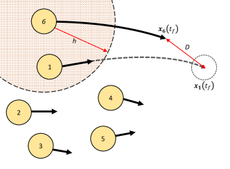
Figure 1: A diagram of a flocking consisting of six agents.

Finally, every agent is also equipped with a long-range sensor, which can estimate the centroid of the flock, given by

$$\mathbf{p}_{cg}(t)=\frac{1}{|\mathcal{N}_{i}(t)|}\sum_{i\in\mathcal{A}}\mathbf{p}_{i}(t),$$ (10)

where $|\cdot|$ denotes set cardinality. The purpose of (10) is to drive isolated agents back toward the flock. This can reasonably be achieved with inexpensive audio or visual sensors in the case where a majority of the agents have already formed an aggregate. However, for the case where there is no clear flock, it may be challenging to determine (10) in practice.

In order to guarantee safety (7), and to calculate (10), agent $i\in\mathcal{A}$ requires information about the trajectories of all agents $j\in\mathcal{N}_{i}(t).$ One potential approach to handle this is to impose a priority ordering on the agents; in this case, higher priority agents act first while lower priority agents must steer to avoid them [22]. Our approach is for each agent to apply model predictive control. Each agent generates an initial unconstrained trajectory for a given time interval $t\in[t_{0},t_{f}],$ where $t_{f}-t_{0}>0$ is the horizon. Then, agent $i$ follows this generated trajectory for some period $\Delta T$, at which point the trajectory is recalculated over the new interval $t\in[t_{0}+\Delta T,t_{f}+\Delta T]$.

In this case, a longer time interval corresponds to a larger planning space at the cost of increased computational complexity. A decrease in the replanning period, $\Delta T$, provides agent $i$ with a better estimate of its neighbors’ trajectories at the cost of more frequent calculations. The trajectory generated by each agent is the outcome of minimizing the flocking error function, defined next.

Definition 2.

For all agents $i\in\mathcal{A}$, the flocking error is defined by the scalar function

$$\Phi(\mathbf{x}_{i},t_{f}) =w_{1}~{}\phi_{d}(\mathbf{x}_{i},t_{f})+w_{2}~{}\phi_{v}(\mathbf{x}_{i},t_{f})$$

$$\hskip 10.00002pt+w_{3}~{}\phi_{a}(\mathbf{x}_{i},t_{f}),$$ (11)

$$\phi_{d}(\mathbf{x}_{i},t_{f}) =||\mathbf{v}_{i}(t_{f})-\mathbf{v}_{d}(t_{f})||^{2},$$ (12)

$$\phi_{v}(\mathbf{x}_{i},t_{f}) =||\mathbf{v}_{i}(t_{f})-\mathbf{v}_{\text{avg}}(t_{f})||^{2},$$ (13)

$$\phi_{a}(\mathbf{x}_{i},t_{f}) =\begin{cases}(||\mathbf{p}_{cg}(t_{f})-\mathbf{p}_{i}(t_{f})||-D)^{2},\hskip 1.00006pt|\mathcal{N}_{i}(t_{0})|=1,\\ \underset{j\in\mathcal{N}_{i}(t_{0})}{\sum}\Big{(}\mathbf{s}_{ij}(t_{f})\cdot\hat{p}_{ij}(t_{f})-D\Big{)}^{2},\\ \hskip 120.00018pt|\mathcal{N}_{i}(t_{0})|>1,\end{cases}$$ (14)

where $w_{1},w_{2},$ and $w_{3}$ are normalizing parameters which weight the influence of velocity control $\phi_{d}(\mathbf{x}_{i},t_{f})$, velocity matching $\phi_{v}(\mathbf{x}_{i},t_{f}),$ and aggregation $\phi_{a}(\mathbf{x}_{i},t_{f})$ in the overall system behavior. The system parameters $\mathbf{v}_{d}(t_{f})$ and $D$ set the desired flock velocity and separating distance between agents. The average agent speed, $\mathbf{v}_{\text{avg}}(t_{f})$, is given by

$$\mathbf{v}_{\text{avg}}(t_{f})=\begin{cases}\dot{\mathbf{p}}_{cg}(t_{f}),&|\mathcal{N}_{i}(t_{0})|=1,\\ \frac{1}{|\mathcal{N}_{i}(t_{0})|}\sum_{j\in\mathcal{N}_{i}(t_{0})}\mathbf{v}_{j}(t_{f}),&|\mathcal{N}_{i}(t_{0})|>1.\end{cases}$$ (15)

The cases in (14) and (15) when $|\mathcal{N}_{i}(t_{0})|=1$ are equivalent to placing a virtual agent at the centroid of the flock for any agent which becomes isolated. This will drive isolated agents toward the centroid by the construction of the flocking error. However, this does not guarantee that a disconnected group of agents will return to the flock if separation occurs.

Each agent generates its energy-optimal trajectory by solving the following decentralized optimal control problem.

Problem 1.

(Minimum-energy flocking)

For every agent $i\in\mathcal{A}$,

$$\min_{\mathbf{u}_{i}(t)} \Big{\{}\Phi(\mathbf{x}_{i},t_{f})+\int_{t_{0}}^{t_{f}}||\mathbf{u}_{i}(t)||^{2}dt\Big{\}}$$ (16)

subject to: $$\eqref{eq:pDynamics},\eqref{eq:vDynamics},\eqref{eq:vConstraint},\eqref{eq:uConstraint},\eqref{eq:noCollide},~{}\mathbf{x}_{i}(t_{0})=\mathbf{x}_{i}^{0},$$

where $\Phi(\mathbf{x}_{i},t_{f})$ is given by Definition 2 and $\mathbf{x}_{i}^{0}$ is the initial state of agent $i$.

By minimizing the $L^{2}$ norm of the control input we expect to see a proportional reduction in energy consumption. To solve Problem 1, we impose the following assumptions.

Assumption 1.

There are no external disturbances or obstacles.

Assumption 1 is imposed to evaluate the idealized performance of the proposed algorithm. This assumption may be relaxed by introducing a measure of robustness into Problem 1.

Assumption 2.

There are no errors or delays with respect to communication and sensing.

The strength of Assumption 2 is application dependent. In general, it has been shown that sparse updates to model predictive control may be sufficient [23].

Assumption 3.

The flock is low-density (only two agents $i,j\in\mathcal{A}$ ever come within distance $|\mathbf{s}_{ij}|=2R$ of each other).

Assumption 3 may be strong, but it is imposed to simplify the solution to the optimal speed profile for two agents that are safety constrained. This assumption may be removed if an order is imposed on the agents rather than using model predictive control [22], and it may be relaxed in cases when a numerical solver can generate the safety-constrained trajectory in real-time.

III Solution Approach

To derive an analytical solution for Problem 1 we use Hamiltonian Analysis. As the case where the state and control constraints, (4) and (5), are active is well studied in the literature [6] we will only consider the safety constrained case.

As a first step, for an agent $i\in\mathcal{A}$, the safety constraint, (7), must be derived until the control input, $\mathbf{u}_{i}(t)$, appears,

$$\mathbf{N}_{i}(t)=\begin{bmatrix}4R^{2}-\mathbf{s}_{ij}(t)\cdot\mathbf{s}_{ij}(t)\\ -\mathbf{s}_{ij}(t)\cdot\dot{\mathbf{s}}_{ij}(t)\\ -\mathbf{s}_{ij}(t)\cdot\ddot{\mathbf{s}}_{ij}-\dot{\mathbf{s}}_{ij}(t)\cdot\dot{\mathbf{s}}_{ij}(t)\end{bmatrix}\leq\mathbf{0}.$$ (17)

The Hamiltonian is then augmented by the final row of $\mathbf{N}_{i}(t)$, which yields

$$H_{i}=||\mathbf{u}_{i}(t)||^{2}+\boldsymbol{\lambda}_{i}^{p}(t)\cdot\mathbf{v}_{i}(t)+\boldsymbol{\lambda}_{i}^{v}(t)\cdot\mathbf{u}_{i}(t)$$

$$-\sum_{j\in\mathcal{N}_{i}}\mu_{i,j}(t)\Big{(}\mathbf{s}_{ij}(t)\cdot\ddot{\mathbf{s}}_{ij}(t)+\dot{\mathbf{s}}_{ij}(t)\cdot\dot{\mathbf{s}}_{ij}(t)\Big{)},$$ (18)

where $\boldsymbol{\lambda}_{i}^{p}(t),\boldsymbol{\lambda}_{i}^{v}(t)$ are the position and velocity covectors, and $\mu_{ij}(t)$ is the Lagrange multiplier with values

$$\mu_{ij}(t)=\begin{cases}\geq 0,&\text{if }{\mathbf{s}_{ij}(t)\cdot\ddot{\mathbf{s}}_{ij}(t)+\dot{\mathbf{s}}_{ij}(t)\cdot\dot{\mathbf{s}}_{ij}(t)}=0,\\ 0,&\text{if }{\mathbf{s}_{ij}(t)\cdot\ddot{\mathbf{s}}_{ij}(t)+\dot{\mathbf{s}}_{ij}(t)\cdot\dot{\mathbf{s}}_{ij}(t)>0}.\end{cases}$$ (19)

To solve (18) for agent $i\in\mathcal{A}$ we consider that (i) all agents $j\in\mathcal{N}_{i}(t)$ satisfy $\mu_{i,j}=0$ or (ii) any agent $j\in\mathcal{N}_{i}(t)$ satisfies $\mu_{i,j}>0$. We then piece the constrained and unconstrained arcs together to arrive at a piecewise-continuous, energy-optimal trajectory. Next, we present the unconstrained motion and boundary conditions followed by our algorithm for constructing an energy-optimal trajectory in real-time.

III-A Unconstrained Motion

The energy-optimal unconstrained trajectories for the position, speed, acceleration, and covectors resulting from (18) over an interval $t\in[t_{1},t_{2}]\subset\mathbb{R}_{\geq 0}$ are [6]

$$\mathbf{p}_{i}(t)= ~{}\frac{1}{6}\mathbf{a}_{i}t^{3}+\frac{1}{2}\mathbf{b}_{i}t+\mathbf{c}_{i}t+\mathbf{d}_{i},$$ (20)

$$\mathbf{v}_{i}(t)= ~{}\frac{1}{2}\mathbf{a}_{i}t^{2}+\mathbf{b}_{i}t+\mathbf{c}_{i},$$ (21)

$$\mathbf{u}_{i}(t)= ~{}\mathbf{a}_{i}t+\mathbf{b}_{i},$$ (22)

$$\boldsymbol{\lambda}^{p}_{i}(t)= ~{}\mathbf{a}_{i},$$ (23)

$$\boldsymbol{\lambda}^{v}_{i}(t)= ~{}-\mathbf{a}_{i}t-\mathbf{b}_{i},$$ (24)

where $\mathbf{a}_{i},\mathbf{b}_{i},\mathbf{c}_{i},\mathbf{d}_{i}\in\mathbb{R}^{2}$ are constants of integration. Equations (20) - (24) contain $8$ unknowns, which are solved using $8$ boundary conditions;

$$\mathbf{x}_{i}(t_{0}) =\mathbf{x}_{i}^{0},$$ (25)

$$\boldsymbol{\lambda}_{i}(t_{f}) =\frac{\partial\Phi(\mathbf{x}_{i},t)}{\partial\mathbf{x}_{i}}\Big{|}_{t_{f}}.$$ (26)

Solving (26) yields

$$\boldsymbol{\lambda}_{i}^{p}(t_{f}) =-2w_{3}\sum_{j\in\mathcal{N}_{i}(t_{0})}\Big{(}\big{(}||\mathbf{s}_{ij}(t_{f})||-D\big{)}\,\mathbf{s}_{ij}(t_{f})\Big{)},$$ (27)

$$\boldsymbol{\lambda}_{i}^{v}(t_{f}) =2w_{2}\Big{(}\mathbf{v}_{i}(t_{f})-\mathbf{v}_{\text{avg}}\Big{)}+2w_{1}\Big{(}\mathbf{v}_{i}(t_{f})-\mathbf{v}_{d}\Big{)}.$$ (28)

We then substitute (6), (23), and (24) into (27) and (28) to solve for $\mathbf{p}_{i}(t_{f})$ and $\mathbf{u}_{i}(t_{f})$. This yields two equations

$$\mathbf{p}_{i}(t_{f}) =\frac{\mathbf{a}_{i}}{2w_{3}\sum_{j}(||\mathbf{s}_{ij}(t_{f})||-D)}+\sum_{j\in\mathcal{N}_{i}}\mathbf{p}_{j}(t_{f}),$$ (29)

$$\mathbf{u}_{i}(t_{f}) =-2w_{2}\Big{(}\mathbf{v}_{i}(t_{f})-\mathbf{v}_{\text{avg}}\Big{)}-2w_{1}\Big{(}\mathbf{v}_{i}(t_{f})-\mathbf{v}_{d}\Big{)},$$ (30)

where $\mathbf{a}_{i}=0$ if the right-hand side of (27) is ever zero.

Equations (25), (26), and (30) give three conditions to solve for the constants $\mathbf{b}_{i}$, $\mathbf{c}_{i}$, and $\mathbf{d}_{i}$ in (20) - (24). The value of $\mathbf{a}_{i}$ can then be found by the solution of (29), which must be computed numerically.

III-B Constrained Motion

To generate the safety-constrained motion of agent $i\in\mathcal{A}$, we require agent $i$ to cooperate with all agents $j\in\mathcal{N}_{i}(t)$ to solve the centralized optimal control problem whenever the collision avoidance constraint becomes active. The agents will then all employ the centralized solution to guarantee collision avoidance.

For any agent $i\in\mathcal{A}$, we define the set $\mathcal{V}_{i}$ as

$$\mathcal{V}_{i}(t)\coloneqq\{j\in\mathcal{N}_{i}(t)~{}|~{}\mu_{ij}(t)>0,~{}j\neq i\}.$$ (31)

Thus, when $\mathcal{V}_{i}\neq\emptyset$ agent $i$ must follow a safety-constrained trajectory. Application of the Euler-Lagrange equations yields

$$\mathbf{u}_{i}(t)= ~{}-\boldsymbol{\lambda}_{i}^{v}(t)-\sum\mu_{ij}(t)\mathbf{s}_{ij}(t),$$ (32)

$$-\dot{\boldsymbol{\lambda}}_{i}^{v}(t)= ~{}\boldsymbol{\lambda}_{i}^{p}(t)+\sum\mu_{ij}(t)\dot{\mathbf{s}}_{ij}(t),$$ (33)

$$-\dot{\boldsymbol{\lambda}}_{i}^{p}(t)= ~{}\sum\mu_{ij}(t)\ddot{\mathbf{s}}_{ij}(t),$$ (34)

which, in general, must be solved numerically. However, under Assumption 3, we may consider the case where only two agents interact. We define

$$a_{ij}(t)\coloneqq||\dot{\mathbf{s}}_{ij}(t)||,$$ (35)

which is the relative speed between the two constrained agents. We may then construct a new basis for $\mathbb{R}^{2}$ which we define next.

Definition 3.

The orthonormal contact basis for any two agents in contact, $i\in\mathcal{A},~{}j\in\mathcal{V}_{i}$, with a nonzero relative speed, is defined as

$$\hat{p}_{ij}(t)\coloneqq ~{}\frac{\mathbf{s}_{ij}(t)}{||\mathbf{s}_{ij}(t)||}=\frac{\mathbf{s}_{ij}(t)}{2R},$$ (36)

$$\hat{q}_{ij}(t)\coloneqq ~{}\frac{\dot{\mathbf{s}}_{ij}(t)}{||\dot{\mathbf{s}}_{ij}(t)||}=\frac{\dot{\mathbf{s}}_{ij}(t)}{a_{ij}(t)},$$ (37)

where $\hat{p}_{ij}(t)\cdot\hat{q}_{ij}(t)=0$ by (17).

To solve the (32) - (34) we will project $\ddot{\mathbf{s}}_{ij}(t)$ onto the contact basis (Definition 3). From (17) we can project $\ddot{\mathbf{s}}_{ij}$ onto $\hat{p}_{ij}$ by

$$\ddot{\mathbf{s}}_{ij}(t)\cdot\mathbf{s}_{ij}(t)=-\dot{s}_{ij}(t)\cdot\dot{s}_{ij}(t)=-a_{ij}^{2}(t).$$ (38)

The projection of $\ddot{\mathbf{s}}_{ij}(t)$ onto $\hat{q}_{ij}(t)$ can be calculated by applying integration by parts, which yields [22],

$$\ddot{\mathbf{s}}_{ij}(t)\cdot\dot{\mathbf{s}}_{ij}(t)=a_{ij}(t)\cdot\dot{a}_{ij}(t).$$ (39)

Therefore, the projection of $\ddot{\mathbf{s}}_{ij}$ onto the contact basis is

$$\ddot{\mathbf{s}}_{ij}(t)=\begin{bmatrix}-a_{ij}^{2}(t)\frac{1}{2R}\\ \dot{a}_{ij}(t)\end{bmatrix}.$$ (40)

Finally, we can use (40) to solve for the time derivatives of (36) and (37). First we have

$$\frac{d}{dt}\hat{p}_{ij}(t)=\frac{\dot{\mathbf{s}}_{ij}(t)}{2R}=\frac{a(t)}{2R}\hat{q}_{ij}(t).$$ (41)

Taking the time derivative of $\hat{q}_{ij}(t)$ and substituting (40) in the numerator yields [22],

$$\frac{d}{dt}\hat{q}_{ij}(t)=-\frac{a(t)}{2R}\hat{p}_{ij}(t).$$ (42)

By (6), we may now write $\ddot{\mathbf{s}}_{ij}(t)$ projected on to the contact basis (Definition 3) as

$$\ddot{\mathbf{s}}_{ij}(t)= ~{}\mathbf{u}_{j}(t)-\mathbf{u}_{i}(t)=-\mathbf{L}_{ij}^{v}(t)+m_{ij}(t)\mathbf{s}_{ij}(t)$$

$$= ~{}-\mathbf{L}_{ij}^{v}(t)\cdot\begin{bmatrix}\hat{p}_{ij}(t)\\ \hat{q}_{ij}(t)\end{bmatrix}+m_{ij}(t)\cdot\begin{bmatrix}2R\\ 0\end{bmatrix},$$ (43)

where $m_{ij}(t)=\mu_{ij}(t)+\mu_{ji}(t)$, and $\mathbf{L}_{ij}^{x}(t)=\boldsymbol{\lambda}_{j}^{x}(t)-\boldsymbol{\lambda}_{i}^{x}(t)$. Next we substitute (38) and (39) into (43) and rewrite it as a system of scalar equations,

$$\mathbf{L}_{ij}^{v}(t)\cdot\hat{p}_{ij}(t) =\frac{a_{ij}^{2}(t)}{2R}+2R~{}m_{ij}(t),$$ (44)

$$\mathbf{L}_{ij}^{v}(t)\cdot\hat{q}_{ij}(t) =-\dot{a}_{ij}(t).$$ (45)

Taking a time derivative yields

$$\dot{\mathbf{L}}_{ij}^{v}(t)\cdot\hat{p}_{ij}(t)+\mathbf{L}_{ij}^{v}(t)\cdot\dot{\hat{p}}_{ij}(t) =\frac{a_{ij}(t)\dot{a}_{ij}(t)}{R}+2R\dot{m}_{ij}(t),$$ (46)

$$\dot{\mathbf{L}}_{ij}^{v}(t)\cdot\hat{q}_{ij}(t)+\mathbf{L}_{ij}^{v}(t)\cdot\dot{\hat{q}}_{ij}(t) =-\ddot{a}_{ij}(t).$$ (47)

Then we substitute (33), (41), and (42) into (46) and (47) which simplifies to

$$\mathbf{L}_{ij}^{p}(t)\cdot\hat{p}_{ij}(t) =-2R~{}\dot{m}_{ij}(t)-\frac{3}{2R}a_{ij}(t)\dot{a}_{ij}(t),$$ (48)

$$\mathbf{L}_{ij}^{p}(t)\cdot\hat{q}_{ij}(t) =\ddot{a}_{ij}(t)-\frac{a_{ij}^{3}(t)}{4R^{2}}.$$ (49)

Repeating this process of deriving and substituting on (48) and (49) yields a pair of coupled nonlinear second-order ordinary differential equations,

$$\frac{4a_{ij}(t)\ddot{a}_{ij}(t)}{2R}+\frac{3\dot{a}^{2}_{ij}(t)}{2R} +2R\ddot{m}_{ij}(t)=\frac{a_{ij}^{4}(t)}{8R^{3}}$$

$$~{}~{}+\frac{m_{ij}(t)a_{ij}^{2}(t)}{2R},$$ (50)

$$m_{ij}(t)\dot{a}_{ij}(t)+\dot{m}_{ij}(t)a_{ij}(t) +\frac{6a_{ij}^{2}(t)\dot{a}_{ij}(t)}{4R^{2}}=\dddot{a}_{ij}(t).$$ (51)

Thus, for any constrained trajectory to be energy-optimal it must be a solution of (50) and (51) while also satisfying the boundary conditions (25) and (26). In general this is difficult, as both equations are nonlinear and (51) is third order.

An alternative solution is to impose $a_{ij}(t)=0$ over any nonzero interval where the safety constraint is active. This implies $\dot{\mathbf{s}}_{ij}(t)=\mathbf{v}_{j}(t)-\mathbf{v}_{i}(t)=0$. Additionally, as $\dot{\mathbf{s}}_{ij}(t)$ is constant, its derivative $\ddot{\mathbf{s}}_{ij}(t)=0$. Thus we may select $\mathbf{v}_{i}(t)=\mathbf{v}_{j}(t)$ and $\mathbf{u}_{i}(t)=\mathbf{u}_{j}(t)$ as a “reigning optimal” solution [24].

To generate a final energy-optimal trajectory, each agent will piece together unconstrained and constrained arcs during each trajectory update. In the following section, we present the decentralized strategy used by each agent to generate collision-free by piecing together energy-optimal motion primitives.

III-C Decentralized Trajectory Generation

To generate the trajectory of each agent we will use the following definition of contact intervals.

Definition 4.

For each agent $i\in\mathcal{A}$ we define $g\in\mathbb{N}$ contact intervals indexed by $k=1,2,...,g$. These $g$ intervals must satisfy

$$\tau_{i}^{k} \subset[t_{0},t_{f}]\text{ such that }$$

$$\mathcal{V}_{i}(t_{a}) =\mathcal{V}_{i}(t_{b})\neq\emptyset~{}~{}\forall~{}t_{a},t_{b}\in\tau_{i}^{k},$$

where for any two intervals $p,q\in\mathbb{N},~{}p\neq q$, we have $t_{p}<t_{q}$ for $t_{p}\in\tau_{i}^{p}$ and $t_{q}\in\tau_{i}^{q}$. The contact intervals correspond to the nonzero and non-overlapping intervals of time where $\mathcal{V}_{i}(t)$ is invariant.

The contact intervals correspond to the instances in time when each agent $i\in\mathcal{A}$ would violate the safety constraint when traveling along an unconstrained trajectory. To guarantee safety, we enforce the centralized solution to the safety-constrained case over these intervals. We then piece these constraints together with the initial and final conditions using unconstrained trajectory segments. Each agent $i\in\mathcal{A}$ performs the following steps simultaneously:

1. Generate an unconstrained trajectory for $t\in[t_{0},t_{f}]$.

2. Exchange unconstrained trajectories with all $j\in\mathcal{N}_{i}(t)$.

3. Calculate $\mathcal{V}_{i}(t)$.

4. Generate a constrained arc for every contact interval (Definition 4) and fix the entry and exit states for each interval.

5. Piece together all constrained arcs using unconstrained trajectories and continuity in $\mathbf{x}_{i}$ at the boundaries.

6. Generate initial and final unconstrained arcs to satisfy $\mathbf{x}_{i}(t_{0})$ and $\mathbf{x}_{i}(t_{f})$.

7. Generate escape arcs, i.e., agent $i$ may exit to an unconstrained trajectory early if it does not violate any safety constraints.

The above steps will be performed by all agents simultaneously and repeated with a period of $\Delta T$ per our control framework.

IV Simulation Results

To validate our decentralized controller we developed two sets of simulations. First, we implemented the controller in MATLAB where the unconstrained and distance-constrained trajectories could be validated on double integrator agents. Next, the controller was applied to a set of AscTec quadrotors in Gazebo. The results of this simulation show that our optimal controller generates high-level trajectories which display emergent flocking behavior. These trajectories are also realizable by the dynamics and low-level flight controller of a commercially available quadrotor.

First, we validated our proposed controller by placing $12$ agents at feasible initial points randomly within the domain in MATLAB. The resultant flocking behavior if presented in Fig. 2; this shows that after a short transient period, a stable flock is formed which moves to the northeast as specified by $\mathbf{v}_{d}$.

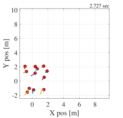
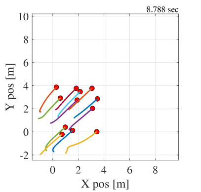
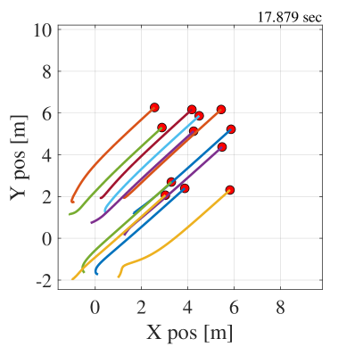
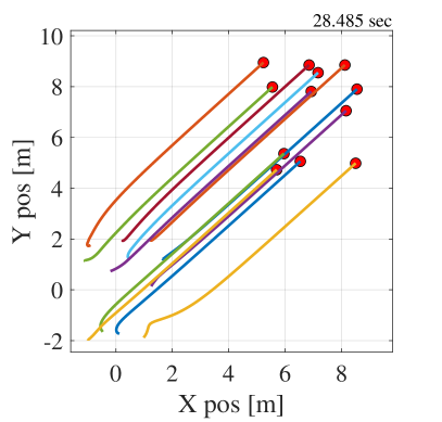
Figure 2: Flocking behavior for 12 agents simulated in MATLAB.

Next, we implemented a sensing-based approximation of the derived optimal control algorithm in Gazebo. This approximation does sacrifice optimality; however, it does not require communication between the agents and it allows an explicit closed-form solution of the boundary conditions. The sensing-based approach for agent $i\in\mathcal{A}$ approximates (29) as

$$\mathbf{p}_{i}(t_{f})= ~{}\sum_{j\in\mathcal{N}_{i}}\mathbf{p}_{j}(t_{0})+\frac{\mathbf{a}_{i}}{2w_{3}\sum_{j}(||\mathbf{s}_{ij}(t_{0})||-D)},$$ (52)

where $\mathbf{p}_{j}(t_{0}),~{}j\in\mathcal{N}_{i}(t_{0})$ must only be sensed by agent $i$. The expected flocking behavior still emerges and is presented in Fig. 3. We implemented our controller in Gazebo using the RotorS package [25] and six AscTec Hummingbirds operating in a horizontal plane. The parameters used for this simulation were: $D=0.25$ m, $\mathbf{v}_{d}=(2.5,0)$ m/s, and $h=4.5$ m. The results of these simulations are visualized in Figs. 3 and 4. In Fig. 3, agents initially coalesce into a hexagonal pattern before flocking along the direction of $\mathbf{v}_{d}$ ($+x$). The flock naturally forms a hexagonal near the end of the simulation due to the relative distance term in the cost function. Figure 4 shows the energy consumption of the agents decaying despite the use of the sensing approximation to estimate neighbor trajectories.

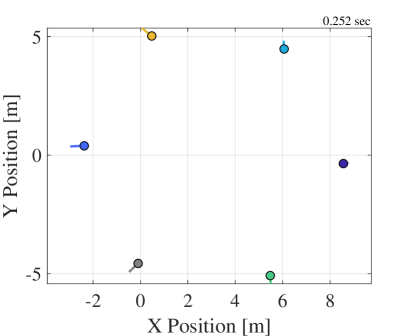
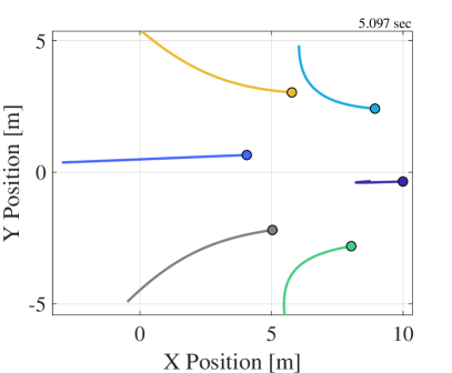
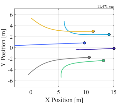
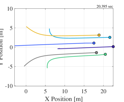
Figure 3: Gazebo simulation with six agents spaced in a hexagonal formation.

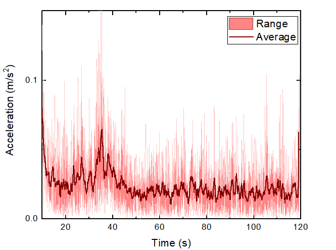
Figure 4: Time series of the average and maximum acceleration magnitude for the six drones.

The Gazebo simulation shows an asymptotic reduction in energy consumption for agents with significantly more complicated dynamics, i.e., drones. Additionally, the sensing-only approximation (52) does not seem to have a significant impact on the global structure of the flock and rate of energy consumption in this scenario.

V Conclusion

In this paper, we proposed an optimal control approach to realize flocking behavior in a group of cooperative agents. We presented the optimal trajectory in the form of a boundary value problem and provided a candidate solution which is locally optimal. Some potential directions for future research include extending the obstacle avoidance constraint to include terrain and mobile obstacles, redefining the aggregation function to use a local description of flocking, and testing the optimal control algorithm on physical hardware in the University of Delaware’s Scaled Smart City.

References

- [1] A. A. Malikopoulos, “A duality framework for stochastic optimal control of complex systems,” IEEE Transactions on Automatic Control, vol. 61, no. 10, pp. 2756–2765, 2016.
- [2] ——, “Centralized stochastic optimal control of complex systems,” in Proceedings of the 2015 European Control Conference, 2015, pp. 721–726.
- [3] ——, “Equilibrium Control Policies for Markov Chains,” in 50th IEEE Conference on Decision and Control and European Control Conference, 2011, pp. 7093–7098.
- [4] A. A. Malikopoulos, V. Maroulas, and J. Xiong, “A multiobjective optimization framework for stochastic control of complex systems,” in Proceedings of the 2015 American Control Conference, 2015, pp. 4263–4268.
- [5] H. Oh, A. R. Shirazi, C. Sun, and Y. Jin, “Bio-inspired self-organising multi-robot pattern formation: A review,” Robotics and Autonomous Systems, vol. 91, pp. 83–100, 2017.
- [6] A. A. Malikopoulos, C. G. Cassandras, and Y. J. Zhang, “A decentralized energy-optimal control framework for connected automated vehicles at signal-free intersections,” Automatica, vol. 93, no. April, pp. 244–256, 2018.
- [7] Q. Lindsey, D. Mellinger, and V. Kumar, “Construction with quadrotor teams,” Autonomous Robots, 2012.
- [8] J. Cortes, “Global formation-shape stabilization of relative sensing networks,” in Proceedings of the American Control Conference, 2009.
- [9] C. W. Reynolds, “Flocks, herds and schools: A distributed behavioral model,” Computer Graphics, vol. 21, no. 4, pp. 25–34, 1987.
- [10] R. Olfati-Saber, “Flocking for multi-agent dynamic systems: Algorithms and theory,” IEEE Transactions on Automatic Control, vol. 51, no. 3, pp. 401–420, 3 2006.
- [11] A. Barve and M. J. Nene, “Survey of Flocking Algorithms in Multi-agent Systems,” International Journal of Computer Science, vol. 19, no. 6, pp. 110–117, 2013.
- [12] S.-J. Chung, A. Paranjape, P. Dames, S. Shen, and V. Kumar, “A Survey on Aerial Swarm Robotics,” IEEE Transactions on Robotics, vol. 34, no. 4, p. 837/855, 2018.
- [13] K.-K. Oh, M.-C. Park, and H.-S. Ahn, “A survey of multi-agent formation control,” Automatica, vol. 53, pp. 424–440, 2015.
- [14] G. Vásárhelyi, C. Virágh, G. Somorjai, T. Nepusz, A. E. Eiben, and T. Vicsek, “Optimized flocking of autonomous drones in confined environments,” Science Robotics, vol. 3, no. 20, 2018.
- [15] H. G. Tanner, A. Jadbabaie, and G. J. Pappas, “Flocking in fixed and switching networks,” IEEE Transactions on Automatic Control, vol. 52, no. 5, pp. 863–868, 2007.
- [16] L. E. Beaver and A. A. Malikopoulos, “A Decentralized Control Framework for Energy-Optimal Goal Assignment and Trajectory Generation,” in Proceedings of the 2019 Conference on Decision and Control, Nice, FR, 2019.
- [17] S. A. Quintero, G. E. Collins, and J. P. Hespanha, “Flocking with fixed-wing UAVs for distributed sensing: A stochastic optimal control approach,” in Proceedings of the American Control Conference, 2013, pp. 2025–2031.
- [18] H. T. Zhang, Z. Cheng, G. Chen, and C. Li, “Model predictive flocking control for second-order multi-agent systems with input constraints,” IEEE Transactions on Circuits and Systems I: Regular Papers, vol. 62, no. 6, pp. 1599–1606, 6 2015.
- [19] V. Gómez, S. Thijssen, A. Symington, S. Hailes, and H. J. Kappen, “Real-Time Stochastic Optimal Control for Multi-agent Quadrotor Swarms,” in 26th International Conference on Automated Planning and Scheduling. London: AAAI Press, 2016, p. 17.
- [20] M. Egerstedt, J. N. Pauli, G. Notomista, and S. Hutchinson, “Robot ecology: Constraint-based control design for long duration autonomy,” pp. 1–7, 1 2018.
- [21] T. Ibuki, S. Wilson, J. Yamauchi, M. Fujita, and M. Egerstedt, “Optimization-Based Distributed Flocking Control for Multiple Rigid Bodies,” IEEE Robotics and Automation Letters, vol. 5, no. 2, pp. 1891–1898, 4 2020.
- [22] L. E. Beaver and A. A. Malikopoulos, “An Energy-Optimal Framework for Assignment and Trajectory Generation in Teams of Autonomous Agents,” Systems & Control Letters (forthcoming), 2020.
- [23] Y. Hu, J. Zhan, and X. Li, “Self-triggered distributed model predictive control for flocking of multi-agent systems,” IET Control Theory & Applications, vol. 12, no. 18, pp. 2441–2448, 12 2018.
- [24] I. M. Ross, A Primer on Pontryagin’s Principle in Optimal Control, 2nd ed., E. Solon, Ed. San Francisco: Collegiate Publishers, 2015.
- [25] F. Furrer, M. Burri, M. Achtelik, and R. Siegwart, “RotorS—A Modular Gazebo MAV Simulator Framework,” in Robot Operating System (ROS): The Complete Reference (Volume 1), A. Koubaa, Ed. Cham: Springer International Publishing, 2016, pp. 595–625.