$\mathbf{\beta}$-delayed proton emission from ¹¹Be in effective field theory

Abstract

We calculate the rate of the rare decay ¹¹Be into ${}^{10}\text{Be}+p+e^{-}+\bar{\nu}_{e}$ using Halo effective field theory, thereby describing the process of beta-delayed proton emission. We assume a shallow $1/2^{+}$ resonance in the ¹⁰Be$-p$ system with an energy consistent with a recent experiment by Ayyad et al. and obtain $b_{p}=4.9_{-2.9}^{+5.6}\text{(exp.)}_{-0.8}^{+4.0}\text{(theo.)}\times 10^{-6}$ for the branching ratio of this decay, predicting a resonance width of $\Gamma_{R}=(9.0^{+4.8}_{-3.3}\text{(exp.)}^{+5.3}_{-2.2}\text{(theo.)})$ keV. Our calculation shows that the experimental branching ratio and resonance parameters of Ayyad et al. are consistent with each other. Moreover, we analyze the general impact of a resonance on the branching ratio and demonstrate that a wide range of combinations of resonance energies and widths can reproduce branching ratios of the correct order. Thus, no exotic mechanism (such as beyond the standard model physics) is needed to explain the experimental decay rate.

Introduction.

Halo nuclei display a large separation of scales between a few loosely bound halo nucleons and a tightly bound core Hansen et al. (1995); Jonson (2004); Riisager (2013); Tanihata (2016). The emergence of the halo degrees of freedom is a fascinating aspect of nuclei away from the valley of stability. The halo nucleons in the core potential spend most of their time in the classically forbidden region outside of the range of the core potential. This is analog to the tunnel effect. But since the halo nucleons are bound to the core, they always have to come back into the core potential. This separation of scales can be used to treat these systems using an effective field theory (EFT) approach called Halo EFT Bertulani et al. (2002); Bedaque et al. (2003); Hammer et al. (2017). Common to all EFTs is that observables are described in a systematic low-energy expansion and that the accuracy of a calculation can be systematically improved. Halo EFT has been applied to a number of observables, including electromagnetic capture reactions and photodissociation processes Hammer and Phillips (2011); Rupak and Higa (2011); Ryberg et al. (2014a); Zhang et al. (2015); Higa et al. (2018); Premarathna and Rupak (2020); Zhang et al. (2020).

Here we will consider, for the first time, the weak decay of the valence neutron of the halo nucleus ¹¹Be into the continuum, ${{}^{11}\text{Be}}\rightarrow{{}^{10}\text{Be}}+p+e^{-}+\bar{\nu}_{e}$, within Halo EFT.

First experimental results for this rare decay mode were presented in Refs. Borge et al. (2013); Riisager (2014). Riisager et al. Riisager et al. (2014) measured a surprisingly large branching ratio for this decay process, $b_{p}=8.3(9)\times 10^{-6}$, which could only be understood in their Woods-Saxon model analysis if the decay proceeds through a new single-particle resonance in ¹¹B. Their measured branching ratio is also more than two orders of magnitude larger than the cluster model prediction by Baye and Tursunov Baye and Tursunov (2011). This led Pfützner and Riisager Pfützner and Riisager (2018) to suggest that $\beta$-delayed proton emission in ¹¹Be is also a possible pathway to detect a dark matter decay mode as proposed by Fornal and Grinstein Fornal and Grinstein (2018). More recently, this branching ratio was remeasured by Ayyad et al. Ayyad et al. (2019) as $b_{p}=1.3(3)\times 10^{-5}$, similar in size to the previous measurement. They also presented new evidence for a low-lying resonance in ¹¹B with resonance energy $E_{R}=0.196(20)$ MeV and width $\Gamma_{R}=12(5)$ keV. Using these parameters, the authors calculated the decay rate in a Woods-Saxon model assuming a pure Gamow-Teller transition. They obtained $b_{p}=8\times 10^{-6}$, which has the correct order of magnitude but is only consistent within a factor of two with their experimental result. The work by Ayyad et al. was criticized in a recent comment by Fynbo et al. Fynbo et al. (2019). A new experiment by Riisager et al. Riisager et al. (2020) gives an upper limit of $b_{p}\leq 2.2\times 10^{-6}$ for the branching ratio but some questions remain due to inconsistencies between different measurements. In conclusion, the branching ratio for $\beta$-delayed proton emission in ¹¹Be remains an important unsolved problem.

The ground state of ¹¹Be is a well-understood $S$-wave halo nucleus. From the ratio of the one-neutron separation energy of ¹¹Be and the excitation energy of the ¹⁰Be core, one can extract the expansion parameter for a description with the core and valence neutron as effective degrees of freedom, $R_{\text{core}}/R_{\text{halo}}\approx 0.4$ Hammer and Phillips (2011). Here $R_{\text{core}}$ and $R_{\text{halo}}$ are the length scales of the core and halo, respectively. In principle, both the ¹⁰Be core and the halo neutron can $\beta$-decay. Since the half-life of the neutron ($T_{1/2}=10$ min) is much shorter than the half-life of the core ($T_{1/2}=10^{6}$ a), it is safe to assume that for $\beta$-delayed proton emission it is always the halo neutron that decays in the halo picture. Therefore, one would naively expect the nucleus to emit this proton due to the repulsive Coulomb interaction: ${{}^{11}\text{Be}}\rightarrow{{}^{10}\text{Be}}+p+e^{-}+\bar{\nu}_{e}$ . This process, called $\beta$-delayed proton emission, has well-defined experimental signatures. However, it is also known that short-distance mechanisms such as the decay into excited states of ¹¹B (that are beyond the halo interpretation) dominate the total $\beta$-decay rate of ¹¹Be Refsgaard et al. (2019); Kelley et al. (2012).

Halo EFT offers a new perspective on $\beta$-delayed proton emission from ¹¹Be by providing a value for the decay rate with a robust uncertainty estimate. It uses the appropriate degrees of freedom and parametrizes the decay observables in terms of a few measurable parameters. Thus, it is perfectly suited for the theoretical description of low-energy processes such as $\beta$-delayed proton emission from halo nuclei. Kong and Ravndal Kong and Ravndal (1999) used these ideas to successfully describe the inverse process of $pp$-fusion into a deuteron and leptons. In contrast to the previous calculation in Ref. Baye and Tursunov (2011), we will use new experimental input parameters and put additional emphasis on the uncertainties associated with using effective degrees of freedom. The halo neutron can $\beta$-decay through both the Gamow-Teller and Fermi operators. The Fermi operator can only connect states in the same isospin multiplet. If all neutrons in ¹¹Be contribute to the $\beta$-decay, this implies that the final state must have $T=3/2$ for a Fermi transition. No such states are currently known in ¹¹B within the $\beta$-decay window. However, due to the halo character of ¹¹Be we expect that only the halo neutron decays, such that the final state has no definite isospin. Thus, we will keep our analysis general and consider both the scenarios of Gamow-Teller and Fermi decay as well a pure Gamow-Teller decay in the following. Specifically, we will show that based on the measured branching ratio, a low-lying resonance is the likely reason for the large partial decay rate, confirming the suggestion of Ref. Riisager et al. (2014). Furthermore, in ¹¹B, we explore the impact of the resonance energy and width on the decay rate and show that the recent results for the resonance energy and width of a low-lying resonance are consistent with the experimentally measured branching ratio.

In order to keep our presentation self-contained, we start by summarizing the concepts of Halo EFT for $S$-wave halo nuclei. We discuss the calculation of decay rates with and without resonant final state interactions and then display our results. Note that these are EFTs for two different scenarios. Formally, we perform calculations up to corrections of order $R_{\text{core}}/R_{\text{halo}}$ in both scenarios but because of the different physics assumptions these cannot be directly compared. We conclude with a summary.

Theoretical foundations.

The Halo EFT Lagrangian $\mathcal{L}$ for ¹¹Be as well as the low-lying resonance in ¹¹B up to next-to-leading order can be written as $\mathcal{L}=\mathcal{L}_{0}+\mathcal{L}_{d}$, where $\mathcal{L}_{0}$ is the free Lagrangian of the ¹⁰Be core, neutron and proton

$$\mathcal{L}_{0}=c^{\dagger} \left(i\partial_{t}+\frac{\nabla^{2}}{2m_{c}}\right)c+n^{\dagger}\left(i\partial_{t}+\frac{\nabla^{2}}{2m_{n}}\right)n$$ (1)

$$+p^{\dagger}\left(i\partial_{t}+\frac{\nabla^{2}}{2m_{p}}\right)p\leavevmode\nobreak\ ,$$

with $c$, $n$ and $p$ the core, neutron and proton fields, respectively. The masses of core, neutron and proton are denoted by $m_{c}=9327.548$ MeV, $m_{n}=939.565$ MeV and $m_{p}=938.272$ MeV. The $S$-wave core-neutron as well as core-proton interaction are described by $\mathcal{L}_{d}$, which reads

$$\mathcal{L}_{d}=d_{\text{Be}}^{\dagger} \left[\eta\left(i\partial_{t}+\frac{\nabla^{2}}{2M_{nc}}\right)+\Delta\right]d_{\text{Be}}$$ (2)

$$+d_{\text{B}}^{\dagger}\left[\tilde{\eta}\left(i\partial_{t}+\frac{\nabla^{2}}{2M_{pc}}\right)+\tilde{\Delta}\right]d_{\text{B}}$$

$$-g\left[c^{\dagger}n^{\dagger}d_{\text{Be}}+\text{H.c.}\right]-\tilde{g}\left[c^{\dagger}p^{\dagger}d_{\text{B}}+\text{H.c.}\right],$$

where $d_{\text{Be}}$ and $d_{\text{B}}$ are dimer fields, with spin indices suppressed, that represent the $J^{P}=1/2^{+}$ ground state of ¹¹Be and the $J^{P}=1/2^{+}$ low-lying resonance in ¹¹B, respectively, while $M_{nc}=m_{n}+m_{c}$ and $M_{pc}=m_{p}+m_{c}$.

The renormalization of the low-energy constants for ¹¹Be has been discussed in Ref. Hammer and Phillips (2011). Here, we will briefly summarize the relevant results to define our notation. Due to the non-perturbative nature of the interaction, we need to resum the self-energy diagrams to all orders. After matching the low-energy constants for ¹¹Be appearing in Eq. (2) to the effective range expansion, we obtain the full two-body $T$-matrix

$$T_{0}(E)=\frac{2\pi}{m_{R}}\left[\frac{1}{a_{0}}-r_{0}m_{R}E-\sqrt{-2m_{R}E-i\epsilon}\right]^{-1}\leavevmode\nobreak\ .$$ (3)

where $m_{R}$ is the reduced mass, and $a_{0}$, $r_{0}$ are the $S$-wave ¹⁰Be$-n$ scattering length and effective range, respectively. The residue at the bound state pole of Eq. (3) is required to calculate physical observables, $Z=\textstyle{\frac{2\pi\gamma_{0}}{m_{R}^{2}}}/(1-r_{0}\gamma_{0})$ , with $\gamma_{0}=(1-\sqrt{1-2r_{0}/a_{0}})/r_{0}\equiv\sqrt{2m_{R}S_{n}}$ the binding momentum of the $S$-wave halo state, and $S_{n}$ the one-neutron separation energy of the halo nucleus.

In order to investigate $\beta$-delayed proton emission from ¹¹Be, we include the weak interaction current allowing transitions of a neutron into a proton, electron and antineutrino which corresponds to the hadronic one-body current. Moreover, we have to consider hadronic two-body currents that appear in the dimer formalism once the effective range is included. The corresponding Lagrangian is given by

$$\mathcal{L}_{\text{weak}}=-\frac{G_{F}}{\sqrt{2}}l_{-}^{\mu}\left(\left(J_{\mu}^{+}\right)^{\text{1b}}+\left(J_{\mu}^{+}\right)^{\text{2b}}\right)\leavevmode\nobreak\ ,$$ (4)

where $l^{\mu}_{-}=\bar{u}_{e}\gamma^{\mu}(1-\gamma^{5})v_{\bar{\nu}}$ and $\left(J_{\mu}^{+}\right)^{\text{1b}}=(V_{\mu}^{1}-A_{\mu}^{1})+i(V_{\mu}^{2}-A_{\mu}^{2})$ denote the leptonic and hadronic one-body currents, respectively. Here the hadronic one-body current is decomposed into vector and axial-vector contributions. At leading order, the contributions to this current are $V_{0}^{a}=N^{\dagger}\frac{\tau^{a}}{2}N$, $A_{k}^{a}=g_{A}N^{\dagger}\frac{\tau^{a}}{2}\sigma_{k}N$, where $|g_{A}|\simeq 1.27$ is the ratio of the axial-vector to vector coupling constants Tanabashi et al. (2018). Terms with more derivatives and/or more fields (many-body currents) will appear at higher orders. The first and second term give the conventional Fermi and Gamow-Teller operators, respectively. Including resonant core-proton final state interactions, we have to take into account a two-body current with known coupling constants which arises from gauging the time derivative of the dimer fields appearing in Eq. (2). It is also decomposed into vector and axial-vector contributions and reads

$$\left(J_{\mu}^{+}\right)^{\text{2b}}=\begin{cases}-d_{\text{B}}^{\dagger}\,d_{\text{Be}}\,\,&\mu=0\leavevmode\nobreak\ ,\\ g_{A}\,d_{\text{B}}^{\dagger}\,\sigma_{k}\,d_{\text{Be}}\,\,&\mu=k=1,2,3\leavevmode\nobreak\ .\end{cases}$$ (5)

In addition, there is also an unknown contribution usually denoted as $L_{1A}$ that normally appears at the same order. However, in the case with Coulomb interaction, this piece is suppressed by $\left(R_{\text{core}}/R_{\text{halo}}\right)^{1/2}$ compared to the two-body current in Eq. (5). Therefore, it contributes only at NNLO allowing us to make predictions up to NLO. Note that our power counting including resonant final state interactions implies a suppression of $\left(R_{\text{core}}/R_{\text{halo}}\right)^{1/2}$ going from order to order instead of $R_{\text{core}}/R_{\text{halo}}$ as in the case without resonant final state interactions.

Weak matrix element and decay rate.

We ignore recoil effects in the $\beta$-decay and take both the Gamow-Teller and Fermi transitions into account. After lepton sums, spin averaging, and partial phase space integration, we obtain the decay rate

$$\Gamma=\frac{G_{F}^{2}(1+3g_{A}^{2})}{4\pi^{5}}\int dp\int dp_{e}p^{2}p_{e}^{2}(E_{0}-E-E_{e})^{2}\\ \times C^{2}(\eta_{e})\leavevmode\nobreak\ \overline{|\mathcal{A}(\mathbf{p})|^{2}}\leavevmode\nobreak\ \Theta(E_{0}-E-E_{e})\leavevmode\nobreak\ ,$$ (6)

where $\mathcal{A}$ is the reduced hadronic amplitude for Gamow-Teller and Fermi transitions whose operator coefficients have been factored out and $\Theta$ is the Heaviside step function. Moreover, ${\bf p}$ is the relative momentum of the outgoing proton and core, while $E=p^{2}/(2m_{R})$ is their kinetic energy. Furthermore, $E_{0}=\Delta m-S_{n}$, where $\Delta m=1.29$ MeV is the mass difference between neutron and proton, and $E_{e}=\sqrt{m_{e}^{2}+p_{e}^{2}}$ is the energy of the electron with $m_{e}=0.511$ MeV denoting the electron mass.

The Sommerfeld factor of the electron is given by

$$C^{2}(\eta_{e})=\frac{2\pi\eta_{e}}{(e^{2\pi\eta_{e}}-1)}\leavevmode\nobreak\ ,$$ (7)

where $\eta_{e}=\alpha ZZ_{e}E_{e}/|\mathbf{p_{e}}|$ with $\alpha=1/137$ the fine structure constant. We use $Z=Z_{p}$ in order to ensure that we reproduce the free neutron decay width in the limit of a vanishing one-neutron separation energy of ¹¹Be. This means that the electron is only interacting with the outgoing proton. For the leading contributions resulting from diagrams (a) and (b) of Fig. 1, we assume this to be a good approximation since the ¹⁰Be core is far away from the decaying valence neutron due to the small one-neutron separation energy. For consistency, we use the same Sommerfeld factor in diagram (c) of Fig. 1 although it contains interactions of all particles at a single space-time point. However, since diagram (c) is subleading, we also expect a deviation of subleading order. In order to confirm this expectation, we have performed an explicit calculation using $Z=Z_{p}+Z_{c}$ for all diagrams, which leads to a change of order 30% in the decay rate. Thus, this effect is beyond the 40% accuracy of our calculation (see below) and would enter at higher orders. If a pure Gamow-Teller transition is considered, the factor $1+3g_{A}^{2}$ is replaced by $3g_{A}^{2}$. This results in a reduction of the decay rate by 17 %.

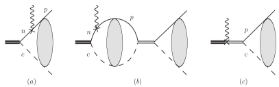
Figure 1: $(a)$: Feynman diagram for the weak decay of a one-neutron halo nucleus into the corresponding core and a proton with Coulomb final state interactions only. $(b)+(c)$: Contributions of resonant final state interactions. The thin double line in the middle denotes the dressed ¹⁰Be$-p$ propagator. The shaded ellipse denotes the Coulomb Green’s function.

Beta-strength sum rule.

The so-called Fermi and Gamow-Teller sum rules (also collectively known as beta-strength sum rule) count the number of weak charges that can decay in the initial state. We will require that this beta-strength sum rule is fulfilled exactly at each order within our EFT power counting. The beta-strenghts are related to the comparative half-life of a decay, the so-called $ft$ value given by

$$ft=\frac{B}{B_{\text{F}}+g_{A}^{2}B_{\text{GT}}}\,,$$ (8)

where $B=2\pi^{3}\ln 2/(m_{e}^{5}G_{F}^{2})$ is the $\beta$-decay constant. In this paper, we will use the value $B=6144.2$ s Pfützner et al. (2012); Hardy and Towner (2005). With $B_{\text{GT}}=3B_{\text{F}}$, we find

$$B_{\text{F}}=\frac{B}{(1+3g_{A}^{2})}\frac{1}{ft}\,.$$ (9)

The inverse $ft$ value is directly related to the transition matrix element $\mathcal{M}$ of ¹¹Be into ${}^{10}\text{Be}+p$,

$$\frac{1}{ft} =\frac{1}{B}\leavevmode\nobreak\ \overline{\left|\mathcal{M}\right|^{2}}$$ (10)

$$=\frac{1}{B}\frac{(1+3g_{A}^{2})}{2\pi^{2}}\int dE\,m_{R}\sqrt{2m_{R}E}\leavevmode\nobreak\ \overline{|\mathcal{A}(\mathbf{p})|^{2}}\,.$$

For a transition into the continuum, the sum rule is exactly fulfilled when integrating the differential beta-strengths

$$\frac{dB_{\text{F}}}{dE} =\frac{1}{2\pi^{2}}\leavevmode\nobreak\ m_{R}\sqrt{2m_{R}E}\leavevmode\nobreak\ \leavevmode\nobreak\ \overline{|\mathcal{A}(\mathbf{p})|^{2}}\,,$$ (11)

$$\frac{dB_{\text{GT}}}{dE} =3\frac{dB_{\text{F}}}{dE}\leavevmode\nobreak\ ,$$ (12)

over the whole continuum leading to the sum rules $B_{\text{F}}=1$ and $B_{\text{GT}}=3$. In the halo picture, we therefore expect beta-strengths $B_{\text{F}}$ and $B_{\text{GT}}$ to be at most $1$ and $3$, respectively, when integrating over the available $Q$-window. At LO where the full non-perturbative solution for a zero-range interaction is used in the incoming as well as outgoing channel, the sum rule is always satisfied. At NLO where range corrections are included, the sum rule puts strong constraints on the ranges in the incoming and outgoing channels such that only certain combinations are allowed.

Hadronic current without resonant final state interactions.

The amplitude for the charge changing weak transition of a two-body system is illustrated as diagram $(a)$ of Fig. 1. It was first calculated in pionless EFT by Kong and Ravndal Kong and Ravndal (1999). The corresponding hadronic current can be written as Ryberg et al. (2014b)

$$\mathcal{A}_{C}^{(a)}(\mathbf{p})=-ig\sqrt{Z}C(\eta_{p})e^{i\sigma_{0}}\frac{2m_{R}}{\mathbf{p}^{2}+\gamma_{0}^{2}}e^{2\eta_{p}\arctan(|\mathbf{p}|/\gamma_{0})}\,,$$ (13)

where $\sigma_{0}$ is the Coulomb phase and $C^{2}(\eta_{p})$ is the Sommerfeld factor from Eq. (7). In the ${}^{10}\text{Be}-p$ system, the Sommerfeld parameter is $\eta_{p}=\alpha Z_{p}Z_{c}m_{R}/|\mathbf{p}|=k_{C}/|\mathbf{p}|$, with $Z_{p}=1$ and $Z_{c}=4$.

Hadronic current with resonant final state interactions.

The current (13) includes only the final state interaction from the exchange of Coulomb photons. We now consider resonant final state interactions whose signature is a low-lying resonance in the ${}^{10}\text{Be}-p$ channel up to NLO. These contributions are shown as diagrams $(b)$ and $(c)$ of Fig. 1. Diagram (c) contributes only at NLO to the amplitude. It arises from a two-body current (with known coupling strength) that appears as a result of the energy-dependent interactions used in the initial state (see Eq. (2)) and the final state (see Ref. Higa et al. (2008)). The thin double line together with the shaded ellipses that represent Coulomb Green’s functions as depicted in diagram $(b)$ essentially combine to the strong scattering amplitude $T_{CS}$ given either in Eq. (14) or (20) Higa et al. (2008); Kong and Ravndal (1999).

The degrees of freedom in Halo EFT are the emitted outgoing proton and ¹⁰Be. Our treatment of the resonance follows Ref. Higa et al. (2008). The corresponding strong scattering amplitude modified by Coulomb corrections is Higa et al. (2008)

$$T_{CS}=\frac{-4\pi/m_{R}}{\left(r_{0}^{C}-\frac{1}{3k_{C}}\right)\left(p^{2}-k_{R}^{2}\right)+\frac{p^{2}}{3k_{C}}-4k_{C}H(\eta_{p})}\leavevmode\nobreak\ ,$$ (14)

where $H(\eta_{p})=\operatorname{Re}[\psi(1+i\eta_{p})]-\ln\eta_{p}+\frac{i}{2\eta_{p}}C^{2}(\eta_{p})$ , with the digamma function $\psi(z)$. The parameters in Eq. (14) are directly related to the complex pole momentum $k^{*}=k_{R}-ik_{I}$:

$$-\frac{1}{a_{0}^{C}} =-\left(r_{0}^{C}-\frac{1}{3k_{C}}\right)\frac{k_{R}^{2}}{2},$$ (15)

$$r_{0}^{C} =-\frac{2\pi k_{C}}{k_{R}k_{I}}\frac{1}{e^{2\pi k_{c}/k_{R}}-1}+\frac{1}{3k_{C}},$$ (16)

where $a_{0}^{C}$ and $r_{0}^{C}$ are the Coulomb-modified scattering length and effective range, respectively. Within our power counting, the parameters $k_{C}$, $k_{R}$, $k_{I}$ as well as $\gamma_{0}$ scale as $1/R_{\text{halo}}$ implying that both Coulomb-modified scattering parameters $a_{0}^{C}$ and $r_{0}^{C}$ scale as $R_{\text{halo}}$. Note that we include $r_{0}^{C}$ despite this scaling only at NLO, since the range $r_{0}$ in the incoming channel scales as $R_{\text{core}}$. The inclusion of both ranges at the same order guarantees that the beta-strength sum rule is satisfied at both LO and NLO.

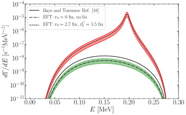
Figure 2: Differential decay rate $d\Gamma/dE$ for $\beta$-delayed proton emission from ¹¹Be as a function of the final-state particle energy $E$. The dash-dotted line shows our EFT result without resonant final state interactions while the solid line gives the result obtained by Baye and Tursunov Baye and Tursunov (2011). The dashed line shows the EFT result including a resonance at $E_{R}=0.196$ MeV in the outgoing channel at NLO. The colored bands give the EFT uncertainty.

The diagrams $(b)$ and $(c)$ of Fig. 1 lead to

$$\mathcal{A}_{CS}^{(b)} =-ig\sqrt{Z}{4m_{R}^{2}}C(\eta_{p})e^{i\sigma_{0}}\mathcal{I}T_{CS}\leavevmode\nobreak\ ,$$ (17)

$$\mathcal{A}_{CS}^{(c)} =-ig\sqrt{Z}{4m_{R}^{2}}C(\eta_{p})e^{i\sigma_{0}}\left(\frac{\sqrt{r_{0}r_{0}^{C}}}{8\pi}\right)T_{CS}\leavevmode\nobreak\ ,$$ (18)

with the complex-valued integral

$$\mathcal{I}=\int\frac{d^{3}\mathbf{q}}{(2\pi)^{3}}\frac{C^{2}(\eta_{q})e^{2\eta_{q}\arctan(|\mathbf{q}|/\gamma_{0})}}{\mathbf{q}^{2}+\gamma_{0}^{2}}\frac{1}{\mathbf{p}^{2}-\mathbf{q}^{2}+i\epsilon}\leavevmode\nobreak\ .$$ (19)

The total amplitude $\mathcal{A}$ is the sum of the amplitudes with and without resonance $\mathcal{A}=\mathcal{A}_{C}^{(a)}+\mathcal{A}_{CS}^{(b)}+\mathcal{A}_{CS}^{(c)}$.

At LO, the Coulomb-modified effective range in the ${}^{10}\text{Be}-p$ system is zero and the amplitude reduces to

$$T_{CS}=-\frac{2\pi}{m_{R}}\left[\frac{1}{-1/a_{0}^{C}-2k_{C}H(\eta_{p})}\right]\leavevmode\nobreak\ .$$ (20)

Results without resonant final state interactions.

We consider two scenarios: beta-delayed proton emission with and without resonant final state interactions from a low-lying resonance in ¹¹B. We start with the first scenario and use the one-neutron separation energy of ¹¹Be $S_{n}=0.5016$ MeV Kelley et al. (2012). In Fig. 2, we plot the differential decay rate $d\Gamma/dE$ as a function of the kinetic energy $E$ of the outgoing hadrons. The solid line gives the result obtained by Baye and Tursunov Baye and Tursunov (2011). The dash-dotted line shows the EFT result with an uncertainty band obtained by adding an uncertainty of order $R_{\text{core}}/R_{\text{halo}}\approx 40$ % from higher order corrections where we use the smallest value of $R_{\text{halo}}$ given by $1/\gamma_{0}$ while we estimate $R_{\text{core}}$ by the effective range $r_{0}$ as a conservative estimate. The remaining curve includes resonant final state interactions and will be discussed below.

For the branching ratio, we obtain $b_{p}=\Gamma/\Gamma_{\rm total}=(1.31\pm 0.51)\times 10^{-8}$ where the EFT uncertainty is again estimated to be of the order of 40 %. Correspondingly, we obtain for the decay rate $\Gamma=(6.6\pm 2.6)\times 10^{-10}\leavevmode\nobreak\ {\rm s}^{-1}$. Baye and Tursunov Baye and Tursunov (2011) obtain $\Gamma=1.5\times 10^{-9}\leavevmode\nobreak\ {\rm s}^{-1}$ which differs by a factor of $2.3$ from our result. We note, however, that they used a Woods-Saxon potential with Coulomb interactions tuned to reproduce ¹¹B properties in the final state. Both theoretical results are significantly smaller than the experimental results reported in Refs. Borge et al. (2013); Riisager (2014); Riisager et al. (2014); Ayyad et al. (2019).

Results with resonant final state interactions.

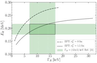
Figure 3: Possible resonance parameter combinations fulfilling the sum rule. The dash-dotted line shows the combinations for $r_{0}=0$ fm at LO corresponding to $r_{0}^{C}=0$ fm while the dashed line shows the combinations for $r_{0}=2.7$ fm at NLO corresponding to $r_{0}^{C}=1.5$ fm. The green bands show the resonance parameters given in Ref. Ayyad et al. (2019).

We now discuss the second scenario including final state interactions. In Fig. 3, we show the possible resonance parameter combinations that fulfill the beta-strength sum rule. The dash-dotted line is the result at LO where the effective range in the incoming channel as well as the Coulomb-modified effective range in the outgoing channel are zero. At NLO, we use $r_{0}=2.7$ fm determined in Ref. Hammer and Phillips (2011) from the measured $B$(E1) strength for Coulomb dissociation of ¹¹Be. The one-neutron separation energy as well as the effective range of ¹¹Be determine the Coulomb-modified effective range in the outgoing channel to be $r_{0}^{C}=1.5$ fm. The sum rule is then satisfied to very good approximation for a wide range of Coulomb-modified scattering lengths in the outgoing channel. The square shows the experimentally measured resonance parameter combinations given in Ref. Ayyad et al. (2019). We note that the value of $r_{0}^{C}$ is determined independently from the experimental resonance parameters. Our NLO curve depicted as the dashed line corresponding to $r_{0}^{C}=1.5$ fm exhibits combinations of $E_{R}$ and $\Gamma_{R}$ that are in agreement with this measurement as indicated by the overlap of the square and the curve.

In Fig. 4, we show the results for the decay rate as a function of the resonance energy at NLO while using the corresponding resonance width that satisfies the sum rule as shown in Fig. 3. The black line represents the decay rate obtained moving along the NLO curve in Fig. 3 while the red shaded envelope gives the theoretical uncertainty estimated from the counterterm contribution in the axial current scaling with $R_{\text{core}}/R_{\text{halo}}\approx 40$ %. The green bands show the experimentally measured branching ratio and resonance energy of Ref. Ayyad et al. (2019). The horizontal blue dashed line denotes the result of the model calculation carried out in Ref. Ayyad et al. (2019) whereas the horizontal blue dash-dotted line gives the upper bound of Ref. Riisager et al. (2020). Comparing our results with Ref. Riisager et al. (2020), we find that resonance energies $E_{R}\geq 0.214$ MeV give results compatible with this upper bound. The corresponding resonance widths can be read off in Fig. 3. When comparing our results with Ref. Ayyad et al. (2019), we find that the low-lying resonance measured in Ref. Ayyad et al. (2019) with $E_{R}=0.196(20)$ MeV and width $\Gamma_{R}=12(5)$ keV is consistent with their experimentally measured branching ratio as indicated by the overlap of the square and the red shaded band. According to Fig. 3, we determine the width corresponding to the resonance energy $E_{R}=0.196(20)$ MeV as $\Gamma_{R}=(9.0^{+4.8}_{-3.3}\text{(exp.)}^{+5.3}_{-2.2}\text{(theo.)})$ keV, which agrees well with the experimental value. At LO, the resonance width scales as $k_{C}^{2}/m_{R}$ whereas at NLO this value is enhanced by a factor of $1/(1-3k_{C}r_{0}^{C})$. This enhancement for Coulomb halos is well known Ryberg et al. (2016); Luna and Papenbrock (2019); Schmickler et al. (2019). Using $E_{R}=0.196(20)$ MeV, we calculate the logarithm of the comparative half-life log$(ft)=3.0$ with $B_{\text{GT}}=2.88$ and $B_{\text{F}}=0.96$ for a decay including both Gamow-Teller and Fermi transitions and log$(ft)=3.1$ with $B_{\text{GT}}=2.88$ for a pure Gamow-Teller transition. The latter result can be compared to log$(ft)=4.8(4)$ calculated by Ayyad et al. Ayyad et al. (2019) which was obtained using a pure Gamow-Teller transition as well, but is significantly larger than our result. This large log$(ft)$ value was also criticized in the comment by Fynbo et al. Fynbo et al. (2019). Ayyad et al. corrected the value to log$(ft)=2.8(4)$ in their recent erratum Ayyad et al. (2019). This new value is now in good agreement with our result. Using the half-life for ¹¹Be given in Ref. Kelley et al. (2012) we convert the Halo EFT result for $E_{R}=0.196(20)$ MeV and $\Gamma_{R}=(9.0^{+4.8}_{-3.3}\text{(exp.)}^{+5.3}_{-2.2}\text{(theo.)})$ keV into the final result for the branching ratio $b_{p}=4.9_{-2.9}^{+5.6}\text{(exp.)}_{-0.8}^{+4.0}\text{(theo.)}\times 10^{-6}$. The corresponding differential decay rate is shown by the dashed line in Fig. 2.

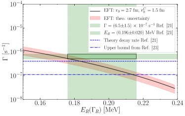
Figure 4: Partial decay rate as a function of the resonance energy at NLO using the corresponding resonance width in accordance with the sum rule (see Fig 3). Explanation of curves and bands is given in inset.

Conclusion.

In this paper, we considered $\beta$-delayed proton emission from ¹¹Be. We compared the scenario with no strong final state interactions with the scenario of a resonant enhancement in the final ¹⁰Be$-p$ channel up to NLO. In the case of no strong final state interactions, we obtained results that are in qualitative agreement with Baye and Tursunov with remaining small differences that can be explained by the different treatment of the final state channel. Including a low-lying resonance with the energy measured in Ref. Ayyad et al. (2019) results in a resonance width and partial decay rate in agreement with this experiment. Thus, our model-independent calculation supports the experimental finding of a low-lying resonance. Furthermore, we have explored the sensitivity of the partial decay rate to the resonance energy and decay width and found that this problem is fine tuned, i.e. only certain combinations of width and resonance energy can reproduce the partial decay rate. In contrast to the model calculation in Ref. Ayyad et al. (2019), we included both, Fermi and Gamow-Teller transitions. However, if a pure Gamow-Teller decay is considered, their partial decay rate can also be reproduced with slightly smaller resonance parameters. Thus, our result implies that ¹¹Be is not a good laboratory to detect dark neutron decays since no exotic mechanism is needed to explain the partial decay rate.

The uncertainties are largely determined by higher order contributions of the EFT expansion. The next contribution within our power counting that we did not include is a counterterm contribution in the axial current scaling with $R_{\text{core}}/R_{\text{halo}}$. Uncertainties of the $S$-wave input parameter (the one-neutron separation energy) do not impact the total uncertainty significantly. Therefore, we estimate the uncertainty in the final decay rate to be approximately $R_{\text{core}}/R_{\text{halo}}\approx 40$ %. Experimental data with higher precision could be used to constrain the ¹⁰Be$-n$ and ¹⁰Be$-p$ interactions. It will be interesting to test whether the inclusion of this resonance changes the Halo EFT predictions for deuteron induced neutron transfer reactions off ¹¹Be which were investigated in Ref. Schmidt et al. (2019).