Deep Video Deblurring: The Devil is in the Details

Abstract

Video deblurring for hand-held cameras is a challenging task, since the underlying blur is caused by both camera shake and object motion. State-of-the-art deep networks exploit temporal information from neighboring frames, either by means of spatio-temporal transformers or by recurrent architectures. In contrast to these involved models, we found that a simple baseline CNN can perform astonishingly well when particular care is taken w.r.t. the details of model and training procedure. To that end, we conduct a comprehensive study regarding these crucial details, uncovering extreme differences in quantitative and qualitative performance. Exploiting these details allows us to boost the architecture and training procedure of a simple baseline CNN by a staggering $3.15$dB, such that it becomes highly competitive w.r.t. cutting-edge networks. This raises the question whether the reported accuracy difference between models is always due to technical contributions or also subject to such orthogonal, but crucial details.

1 Introduction

Blind image deblurring – the recovery of a sharp image given a blurry one – has been studied extensively [25, 27, 40, 45, 50, 55, 56]. However, more recently and perhaps with the increasing popularity of hand-held video cameras, attention has shifted towards deblurring videos [34, 46]. With the (re-)emergence of deep learning and the availability of large amounts of data, the best performing methods today are usually discriminatively trained CNNs [3], RNNs [51], or a mixture thereof [21, 22]. While the “zoo” of video deblurring models differs quite significantly, explanations as to why one network works better than another often remain at an unsatisfactory level. While the performance of state-of-the-art video deblurring methods is usually validated by training within-paper models under the same conditions, the specifics of the training settings between papers remain rather different.

In this work we show that some of these seemingly small details in the model setup and training procedure add up to astonishing quantitative and visual differences. In fact, our quantitative evaluation raises the question whether the benefit for some state-of-the-art models comes from the proposed architectures or perhaps the setup details. This mirrors observations in other areas of computer vision, where the significance of choosing the right training setup is crucial to achieve highly competitive models [48].

Henceforth, we conduct a study on how the model setup and training details of a comparatively simple baseline CNN drastically influence the resulting image quality in video deblurring. By finding the right settings, we unlock a significant amount of hidden power of this baseline, and achieve state-of-the art results on popular benchmarks.

Our systematic analysis considers the following variations: (1) We investigate the use of $\operatorname{linear}$ output layers instead of the typical $\operatorname{sigmoids}$ and consider different initialization methods. Our new $\operatorname{fan\_max}$ initialization combined with $\operatorname{linear}$ outputs already yields a substantial $2$dB benefit over our $\operatorname{sigmoid}$ baseline. (2) While recent work proposes to deblur in YCbCr color space [57], we show that there is no significant benefit over RGB. Instead, a simple extension of the training schedule can lead to an additional $0.4$dB benefit. (3) We uncover that both photometric augmentations as well as random image scaling in training hurt deblurring results due to the mismatch of training vs. test data statistics. The misuse of augmentations can diminish the generalization performance up to a severe 0.44dB. (4) We explore the benefits of using optical flow networks for pre-warping the inputs, which yields another 0.4dB gain. Concatenating pre-warped images to the inputs improves over a simple replacement of the temporal neighbors by up to $0.27$dB. This is in contrast to previous work, which either claimed no benefit from using pre-warping [46], or applied a complex spatio-temporal subnetwork with additional trainable weights [22]. (5) We explore the influence of training patch size and sequence length. Longer sequences yield only a minor benefit, but large patch sizes significantly improve over small ones by up to $0.9$dB. Taken together, we improve our baseline by a striking $3.15$dB and the published results of [46] by $2.11$dB, reaching and even surpassing the quality of complex state-of-the-art networks on standard datasets.

2 Related Work

Classic uniform and non-uniform deblurring.

Classic uniform deblurring methods that restore a sharp image under the assumption of a single blur kernel usually enforce sparse image statistics, and are often combined with probabilistic, variational frameworks [4, 9, 28, 29, 33]. Less common approaches include the use of self-similarity [32], discriminatively trained regression tree fields [43], a dark-channel prior [37], or scale normalization [17].

Moving objects or a moving camera, on the other hand, significantly complicate deblurring, since the motion varies across the image domain. Here, usually restricting assumptions are enforced on the generative blur, either in the form of a candidate blur model [6, 18], a linear blur model [10, 19], or a more generic blur basis [12, 14, 54, 58].

Classic video deblurring. Early work on video blurring [5, 31] proposes to transfer sharp pixels from neighboring frames to the central reference frame. While Matsushita et al. [31] apply a global homography, Cho et al. [5] improve on this by local patch search. Overall, the averaging nature of these approaches tends to overly smooth results [7]. Delbracio et al. [7] overcome this via a weighted average in the Fourier domain, but rely on a registration of neighboring frames, which may fail for large blurs. Kim et al. [20] propose an energy-based approach to jointly estimate optical flow along a latent sharp image using piece-wise linear blur kernels. Later, Ren et al. [42] incorporate semantic segmentation into the energy. Both approaches rely on primal-dual optimization, which is computationally demanding.

Deep image deblurring. Among the first deblurring methods in the light of the recent renaissance of deep learning has been the work by Sun et al. [49] who train a CNN to predict pixelwise candidate blur kernels. Later, Gong et al. [11] extend this from image patches to a fully convolutional approach. Chakrabarti [1] tackles uniform deblurring in the frequency domain by predicting Fourier coefficients of patch-wise deconvolution filters. Note that, as in the classical case, all aforementioned methods are still followed by a standard non-blind deconvolution pipeline. This restriction is lifted by Schuler et al. [44] who replace both the kernel and image estimator module of classic pipelines by neural network blocks, respectively. Noroozi et al. [36] propose a multi-scale CNN, which directly regresses a sharp image from a blurry one. Tao et al. [51] suggest a scale-recurrent neural network (RNN) to solve the deblurring problem at multiple resolutions in conjunction with a multi-scale loss.

Deep image deblurring via GANs. Other approaches draw from the recent progress on generative adversarial networks (GANs). Ramakrishnan et al. [41] propose a GAN for recovering a sharp image from a given blurry one; the generator aims to output a visually plausible, sharp image, which fools the discriminator into thinking it comes from the true sharp image distribution. Nah et al. [34] propose a multi-scale CNN accompanied by an adversarial loss in order to mimic traditional course-to-fine deblurring techniques. Similarly, Kupyn et al. [26] apply a conditional GAN, where the content (or perceptual) loss is notably defined in the domain of CNN feature maps rather than output color space. We do not consider the use of adversarial networks here, as we argue that the accuracy of feed-forward CNNs is not yet saturated on the deblurring task. Note that despite the simplicity of our baseline, we outperform the model of [26] by a large margin, c.f. Sec. 4.

Deep video deblurring. Deep learning approaches to video deblurring have yielded tremendous progress in speed and image quality. Kim et al. [21] focus on the temporal nature of the problem by applying a temporal feature blending layer within an RNN. Similarly, Nah et al. [35] apply an RNN to propagate intra-frame information. While RNNs are promising, we note that these are often difficult to train in practice [38]. We do not rely on a recurrent architecture, but a plain CNN, achieving very competitive results. Zhang et al. [57] use spatio-temporal 3D convolutions in the early stages of a deep residual network. Chen et al. [3] extend [26] with a physics-based reblurring pipeline, which constructs a reblurred image from the sharp predictions using optical flow, and subsequently enforces consistency between the reblurred image and the blurry input image. Wang et al. [52] apply deformable convolutions along an attention module to tackle general video restoration tasks.

The DBN model of Su et al. [46] serves as baseline model in our study. DBN is a simple encoder-decoder CNN with symmetric skip connections; its input is simply the concatenation of the temporal window of the video input sequence. Later, Kim et al. [22] extend the DBN model by a 3D spatio-temporal transformer, which transforms the inputs to the reference frame. Note that this requires training an additional subnetwork that finds 3D correspondences of the inputs to the reference frame. We find that we can outperform [22] based on the same backbone network without the need of a spatial transformer network. More generally, we uncover crucial details in the model and training procedure, which strikingly boost the accuracy by several dB in PSNR, yielding a method that is highly competitive.

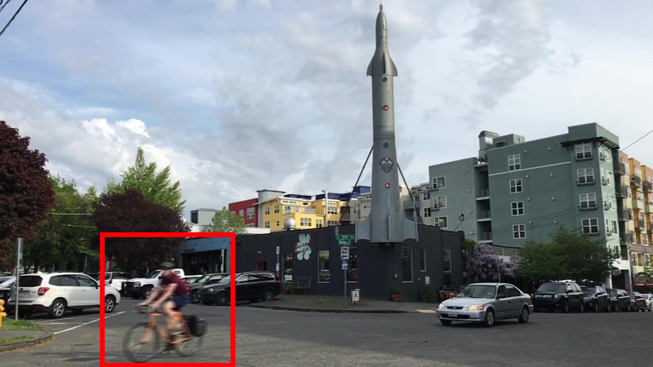
(a) Input

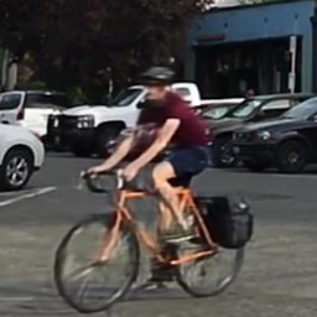
(b) lin+$\operatorname{fan\_max}$

(c) sigm+$\operatorname{fan\_max}$

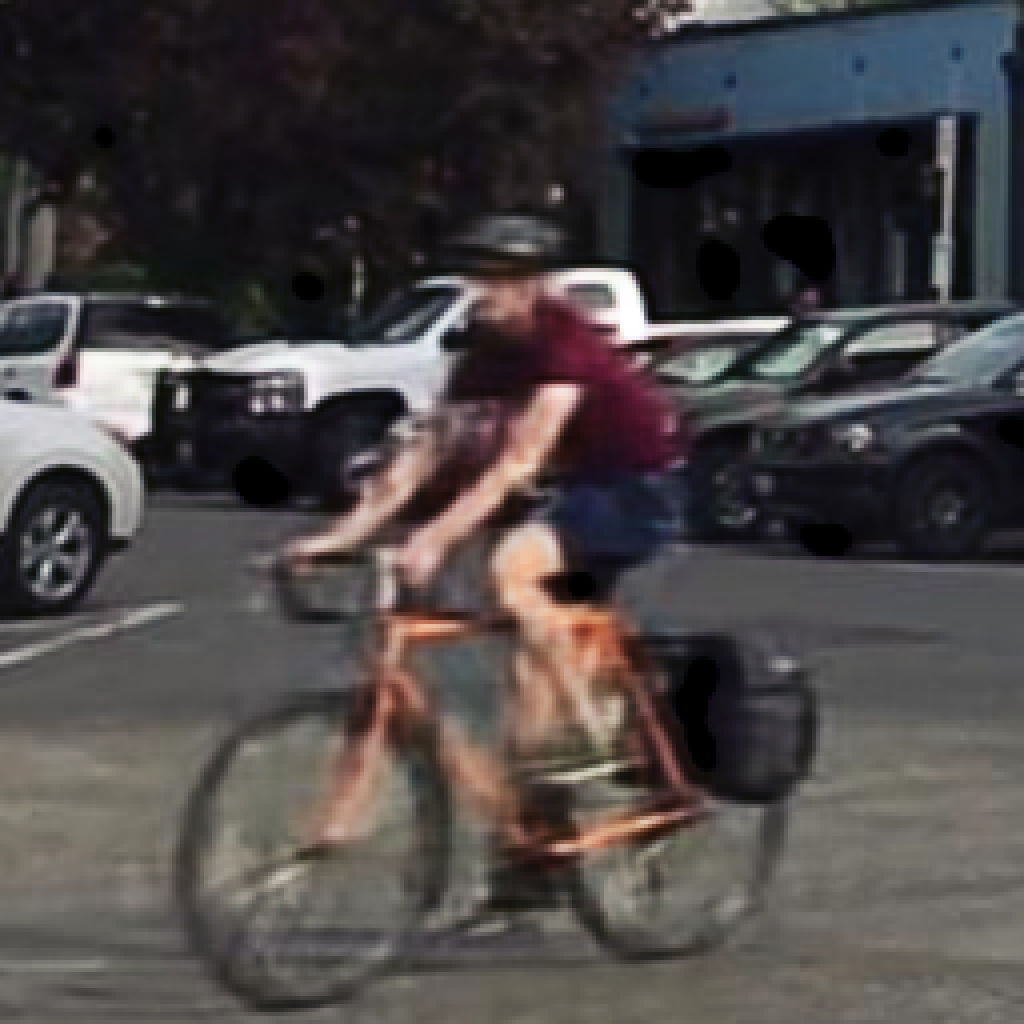
(d) sigm+$\operatorname{fan\_in}$

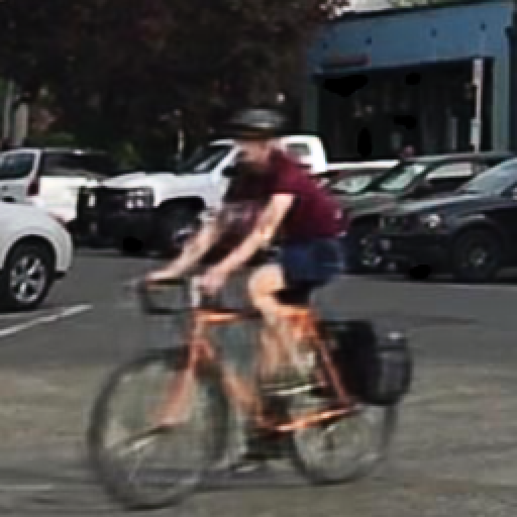
(e) sigm+$\operatorname{fan\_out}$

(f) gt

Figure 1: Varying output layers and initializations. For the input 1(a), a $\operatorname{linear}$ output and $\operatorname{fan\_max}$ initialization 1(b) visually yields better results than a $\operatorname{sigmoid}$ layer, independent of the fan-type used in the initialization. Note the artifacts on the wheel in 1(c) – 1(e).

3 The Details of Deep Video Deblurring

As has been observed in papers in several areas of deep learning and beyond, careful choices of the architecture, (hyper-)parameters, training procedure, and more can significantly affect the final accuracy [2, 30, 40, 48]. We show that the same holds true in deep video deblurring. Specifically, we revisit the basic deep video deblurring network of Su et al. [46] and will uncover step-by-step, how choices made in mode, training, and preprocessing affect the deblurring accuracy. All together, these details add up to a very significant $3.15$dB difference on the test dataset.

3.1 Baseline network

The basis architecture of our study is the DBN network of Su et al. [46] (c.f. Table 1 therein), a fairly standard CNN with symmetric skip connections. We closely follow the original training procedure in as far as it is specified in the paper [46]. Since we focus on details including the training procedure here, we first summarize the basic setup. The baseline model and all subsequent refinements are trained on the 61 training sequences and tested on the 10 test sequences of the GOPRO dataset [46]. The sum of squared error (SSE) loss is used for training and minimized with Adam [23], starting at a learning rate of $0.005$. Following [46], the batch size is taken as 64 where we draw 8 random crops per example. For all convolutional and transposed convolutional layers, 2D batch normalization [16] is applied and initialized with unit weights and zero biases. While this simple architecture has led to competitive results when it was published in 2017, more recent methods [3, 22] have strongly outperformed it. In the following, we explore the potential to improve this baseline architecture and perform a step-by-step analysis. Table 1 gives an overview.

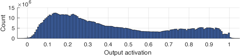
Figure 2: Output activation statistics over test dataset. Even with linear outputs, the $\operatorname{\text{SSE}}$ loss confines most activations to $[0,1]$.

3.2 Detail analysis

Output activation.

The DBN network [46] uses a $\operatorname{sigmoid}$ output layer to yield color values in the range $[0,1]$. Given the limited range of pixel values in real digital images, this appears to be a prudent choice at first glance. We question this, however, by recalling that $\operatorname{sigmoid}$ nonlinearities are a common root of optimization issues due to the well-known vanishing gradient problem. We thus ask whether we need the $\operatorname{sigmoid}$ nonlinearity.

To that end, we replace it with a simple $\operatorname{linear}$ output. As we can see in Table 1(a vs. d), this yields a very substantial 1dB accuracy benefit, highlighting again the importance of avoiding vanishing gradients. In fact, the restriction to the unit range does not pose a significant problem even without output nonlinearity, since the SSE loss largely limits the linear outputs to the correct range anyway. This is illustrated in Fig. 2, which shows the linear activations on the test dataset after training with linear output activations under a $\operatorname{\text{SSE}}$ loss; only very few values lie outside the valid color value range. This can be easily addressed by clamping the outputs to $[0,1]$ at test time.

Initialization. The choice of initialization is not discussed in [46]. However, as for any nonlinear optimization problem, initialization plays a crucial role. Indeed, we find that good initialization is necessary to reproduce the results reported in [46]. Perhaps, the most popular initialization strategy for $\operatorname{relu}$-based neural networks today is the $\operatorname{msra}$ method of He et al. [13]. It ensures that under $\operatorname{relu}$ activations, the magnitudes of the input signal do not exponentially increase or decrease. The $\operatorname{msra}$ initialization method typically comes in two variants, $\operatorname{msra}+\operatorname{fan\_in}$, and $\operatorname{msra}+\operatorname{fan\_out}$, depending on whether signal magnitudes should be preserved in the forward or backward pass. In practice, $\operatorname{fan\_in}$ and $\operatorname{fan\_out}$ correspond to the number of gates connected to the inputs and outputs. We additionally propose $\operatorname{fan\_max}$, which we define as the maximum number of gates connected to either the inputs or outputs, providing a trade-off between $\operatorname{fan\_in}$ and $\operatorname{fan\_out}$. For hourglass architectures, it is typical to increase the number of feature maps in the encoding part; here, $\operatorname{fan\_max}$ adapts to the increasing number of feature maps via $\operatorname{fan\_out}$ initialization. The decoder is effectively initialized by $\operatorname{fan\_in}$ to accommodate the decreasing number of feature maps.

Table 1(a – f) evaluates these initializations in conjunction with $\operatorname{linear}$ and $\operatorname{sigmoid}$ outputs layers. Due to the attenuated gradient, all three $\operatorname{sigmoid}$ variants are worse than any $\operatorname{linear}$ output layer. On the other hand, $\operatorname{linear}$ in conjunction with $\operatorname{fan\_max}$ initialization works much better than the traditional $\operatorname{fan\_in}$ and $\operatorname{fan\_out}$ initializations, yielding a $\sim$0.7dB benefit. The visual results in Fig. 1 also reveal that the $\operatorname{linear}$ output contains fewer visual artifacts.

Verdict: For a color prediction task such as deblurring, $\operatorname{sigmoids}$ should be replaced by $\operatorname{linear}$ outputs. We recommend considering a $\operatorname{fan\_max}$ initialization as an alternative to $\operatorname{fan\_in}$ and $\operatorname{fan\_out}$.

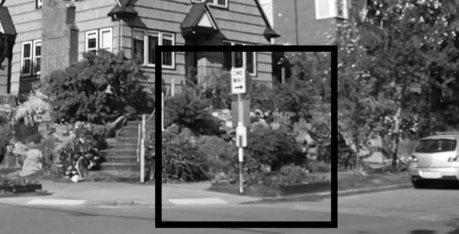
(a) GT Y

(b) Blurry CbCr

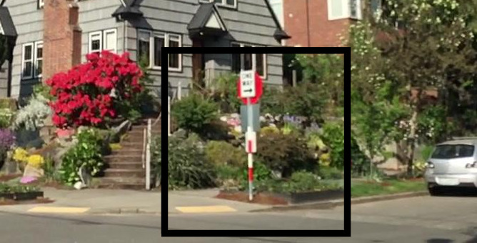
(c) GT RGB

(d) Reconstructed RGB

Figure 3: Oracle experiment in YCbCr color space. Deblurring in YCbCr color space combines 3(a) the sharp Y channel (here, ground truth) with 3(b) the blurry CbCr channel. The reconstruction 3(d) is quantitatively close to the RGB ground truth 3(c), yet suffers from halo artifacts for very blurry regions, as highlighted.

Color space. In classic deblurring color channels are typically deblurred separately. While this is clearly not necessary in deep neural architectures – we can just output three color channels simultaneously – the question remains whether the RGB color space is appropriate. Zhang et al. [57] propose to convert the blurry input images to YCbCr space, where Y corresponds to grayscale intensities and CbCr denotes the color components, c.f. Fig. 3. The sharp image is subsequently reconstructed from the deblurred Y channels and the blurry input CbCr channels. This effectively enforces a natural upper bound on the problem, i.e. computing the average PSNR value of the test dataset yields

$$\text{PSNR}(\text{RGB}_{\text{input}},\text{RGB}_{\text{gt}}) =27.23\text{dB}$$ (1a)

$$\text{PSNR}(\text{cat}(\text{Y}_{\text{gt}},\text{CbCr}_{\text{input}}),\text{RGB}_{\text{gt}}) =56.26\text{dB}.$$ (1b)

That is, an oracle with access to the ground truth $Y$ channel can achieve at most $56.26$dB PSNR. Hence, the natural upper bound does not pose a real quantitative limitation, since $56.26$dB is much better than any current method can achieve. In practice, however, we found that the benefit of solving the problem in YCbCr space is not significant. Table 1(f, g) show a minimal $\sim$0.01dB benefit of using YCbCr over RGB. YCbCr can still be useful as it allows for models with a smaller computational footprint, since fewer weights are required in the first and last layer. Here, we want to raise another problem of YCbCr deblurring: For very blurry regions, the reconstruction even from the ground truth Y channel may contain halo artifacts as depicted in Fig. 3(d).

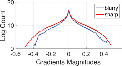
(a) Original statistics

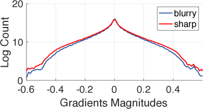
(b) Statistics under rescaling

Figure 4: Gradient statistics under rescaling. Rescaling the images as part of the augmentation is problematic due to the changed degradation statistics (blue – blurry image statistics, red – sharp image statistics). The difference between the plots in unscaled 4(a) vs. rescaled images 4(b) is apparent.

Training schedule. As observed in other works, e.g. [15], longer training schedules can be beneficial for dense prediction tasks. Here, we apply two different training schedules, a short one with 116 epochs resembling the original schedule [46] by halving the learning rate at epochs $[32,44,56,68,80,92,104]$, as well as a long schedule with 216 epochs, halving the learning rate at epochs $[108,126,144,162,180,198]$. To obtain the long training schedule, we initially inspected the results of running PyTorch’s ReduceLROnPlateau scheduler (with patience=10, factor=0.5) for an indefinite time, where we subsequently scheduled the epochs in which learning rates drop in equidistant intervals (here 18). The longer training schedule improves both the RGB and YCbCr networks roughly by 0.4dB, c.f. Table 1(f – i). Since the benefit of YCbCr is rather small for both short and long schedule, we conduct the remaining experiments in RGB space. Figure 5 shows the visual differences between RGB and YCbCr deblurring. While the perceptual differences between RGB and YCbCr are not significant, the long schedules improve the readability of the letters over the short ones.

(a) Input

(b) rgb+short

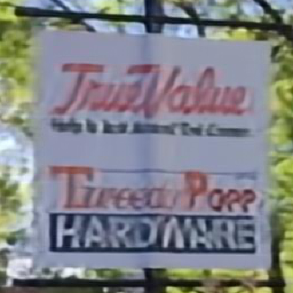
(c) ycbcr+short

(d) rgb+long

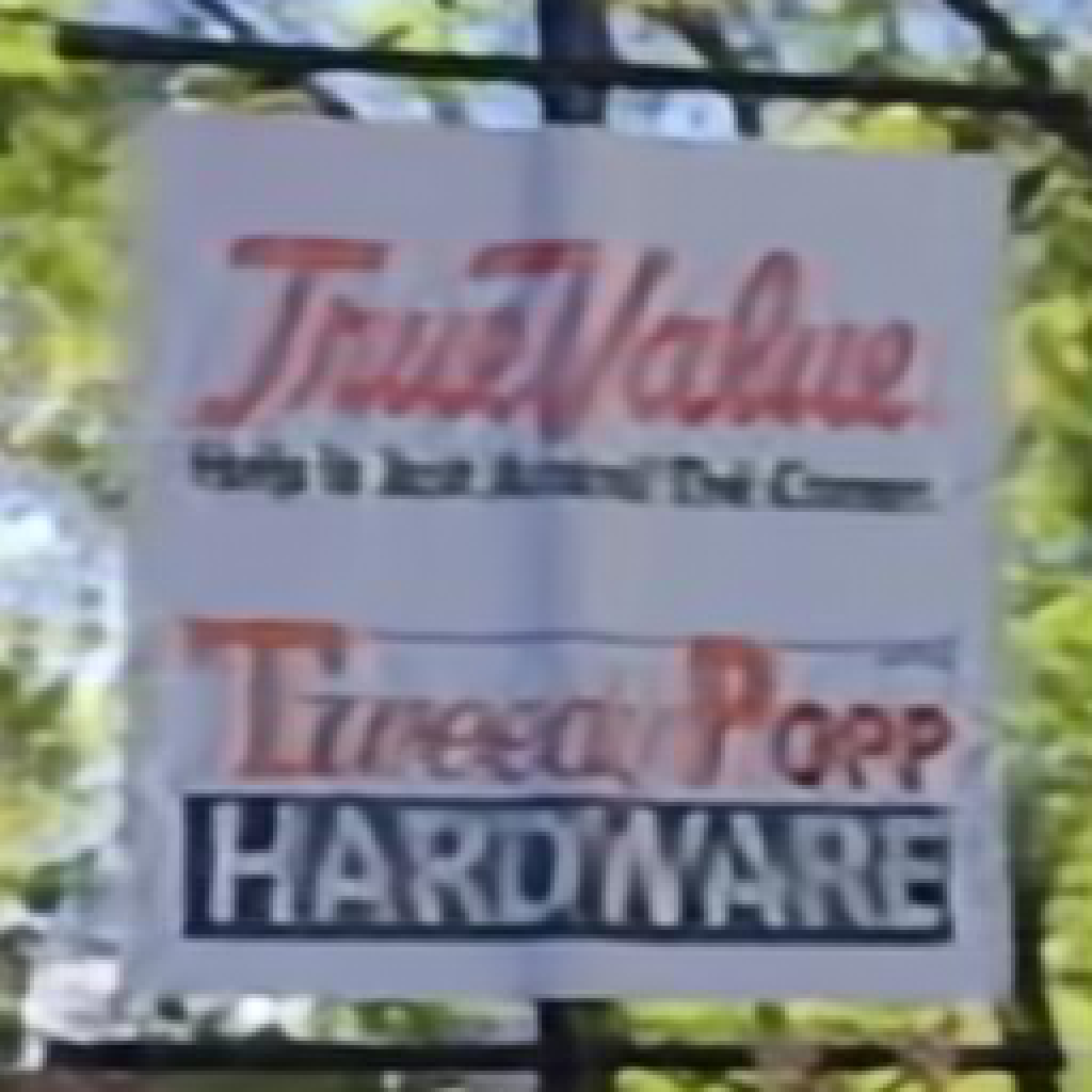
(e) ycbcr+long

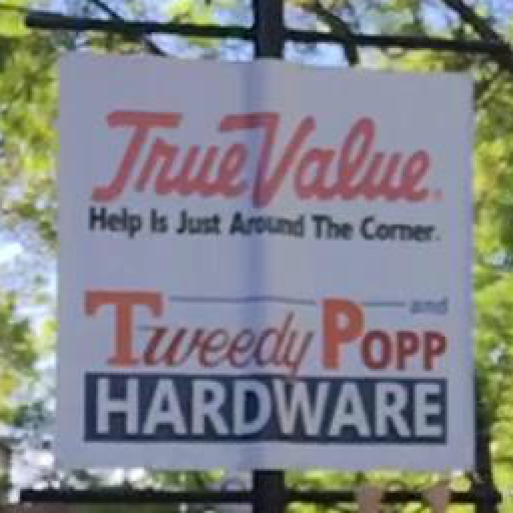
(f) gt

Figure 5: Color space and training schedule. The difference of RGB deblurring 5(b) and YCbCr deblurring 5(c) is minimal. However, using a long training schedule 5(d) and 5(e) significantly boosts performance of both. Note how the last letters of ’HARDWARE’ become visibly clearer with the long training schedule.

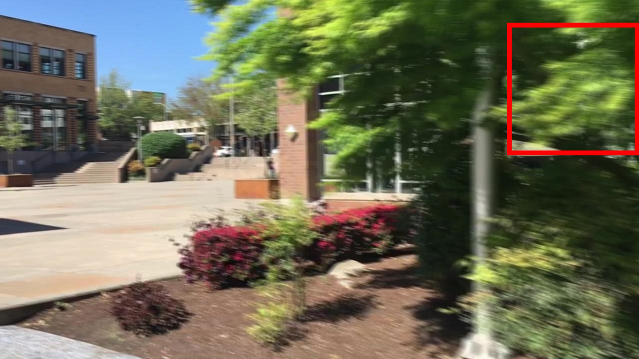
(a) Input

(b) photom.

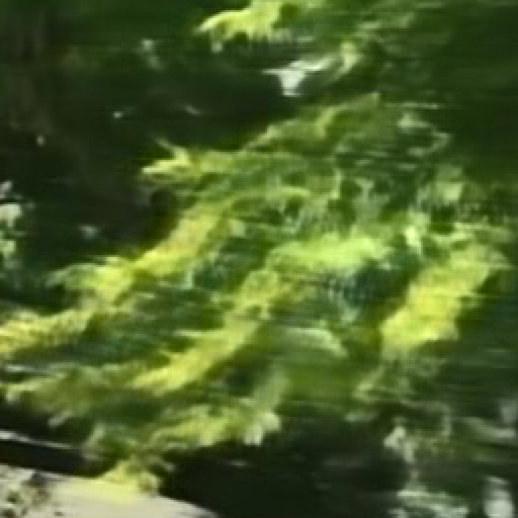
(c) scales

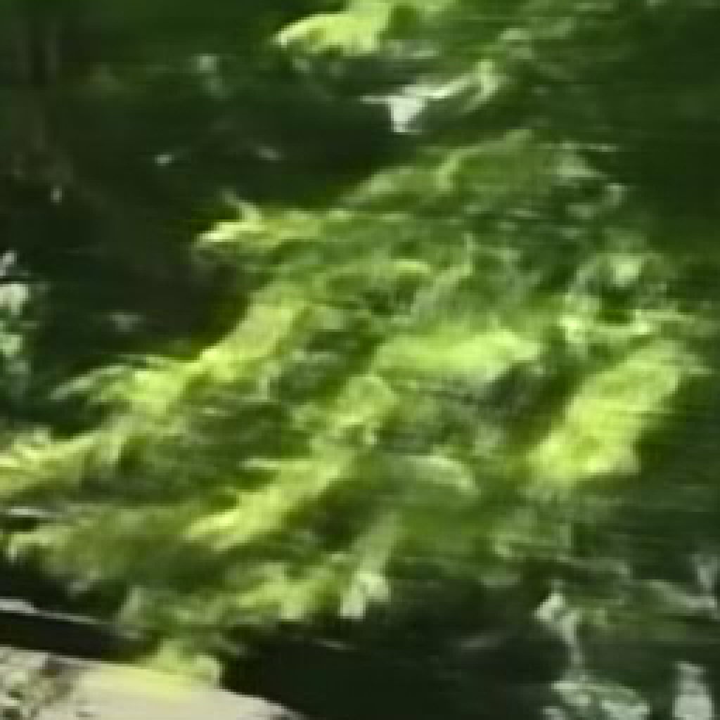
(d) photom.+scales

(e) no augm.

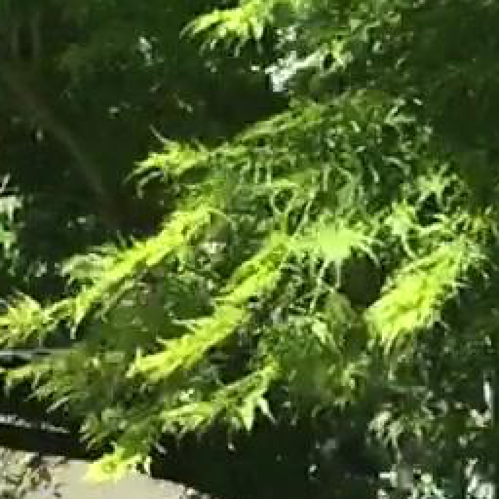
(f) gt

Figure 6: Varying photometric augmentations and scales. Both photometric augmentations and random scales 6(b), 6(c) have a negative impact on image quality. The differences are subtle but visually apparent in blobs; compare, e.g., the central part of 6(d) with 6(e).

Verdict: YCbCr does not present a significant benefit over RGB; it is, however, viable for very large models, if model size is an issue. Very blurry training examples may be suboptimal, since even the oracle $Y$ channel yields halo artifacts. Similar to other dense prediction tasks, long training schedules yield significant benefits.

Photometric augmentation and random scales. Data augmentation plays a crucial role in many dense prediction tasks such as optical flow [8]. However, it is often disregarded from the analysis of deblurring methods. More precisely, while our baseline [46] and recent work [22, 57] all train under random rotations ($0^{\circ},90^{\circ},180^{\circ},270^{\circ}$), random horizontal and vertical flips, and random crops (usually of size $128^{2}$), other types of augmentations such as photometric transformations and random scaling are not agreed upon. Su et al. [46] train their model under random image scales of $[\nicefrac{{1}}{{4}},\nicefrac{{1}}{{3}},\nicefrac{{1}}{{2}}]$, yet Zhang et al. [57] do not rescale the training images. Here, we explore the influence of both random photometric transformations and random scales.

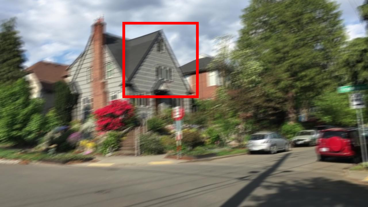
(a) Input

(b) no flow

(c) f1s+rep

(d) pwc+rep

(e) pwc+cat

(f) gt

Figure 7: Optical flow prewarping. Prewarping with optical flow positively influences image quality. We experiment with FlowNet1S 7(c), and PWC-Net 7(d), 7(e). Concatenating warped images with the inputs 7(e) produces fewer visual artifacts than just replacing the temporal neighbors 7(d). Here all flow variants reconstruct the horizontal structures much better than the baseline without pre-warping 7(b).

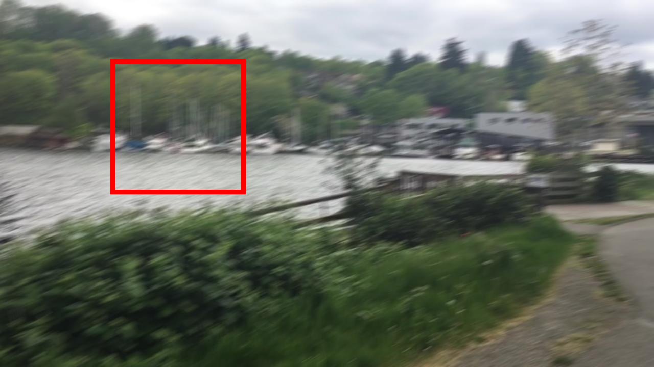
(a) Input

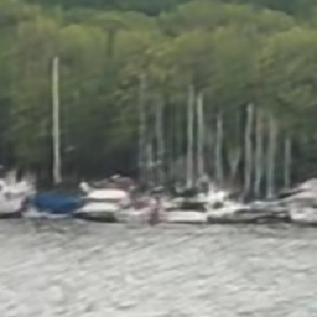
(b) 64x64

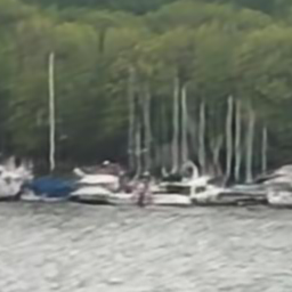
(c) 128x128

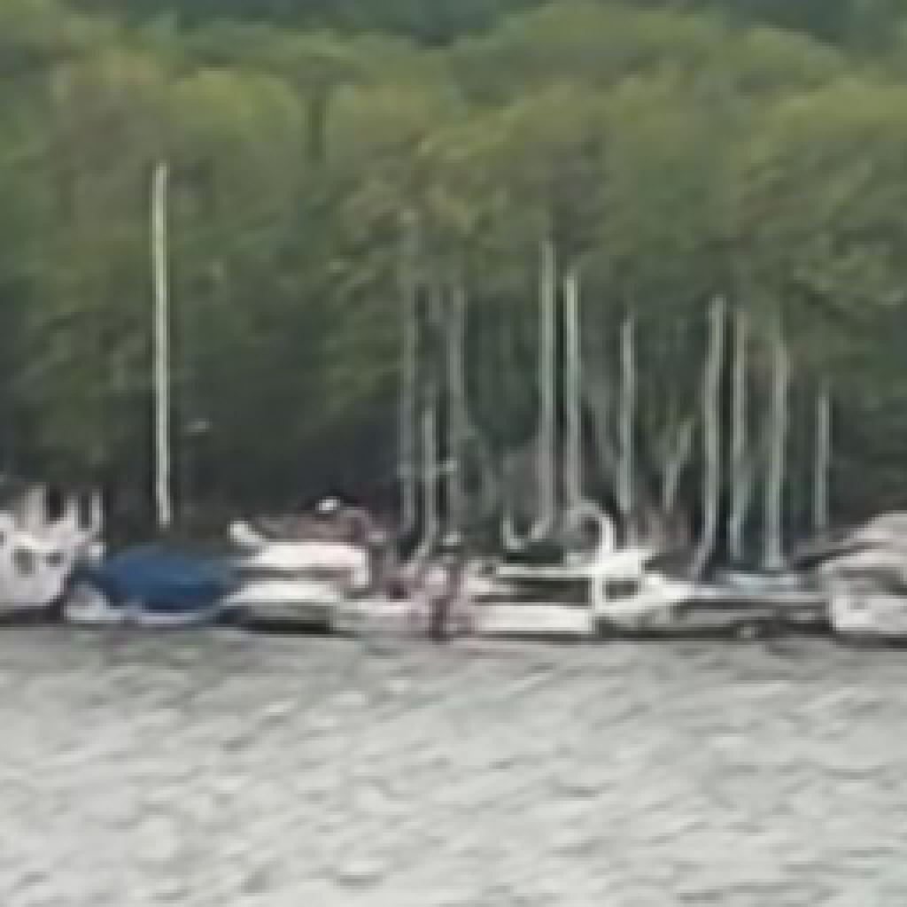
(d) 160x160

(e) 192x192

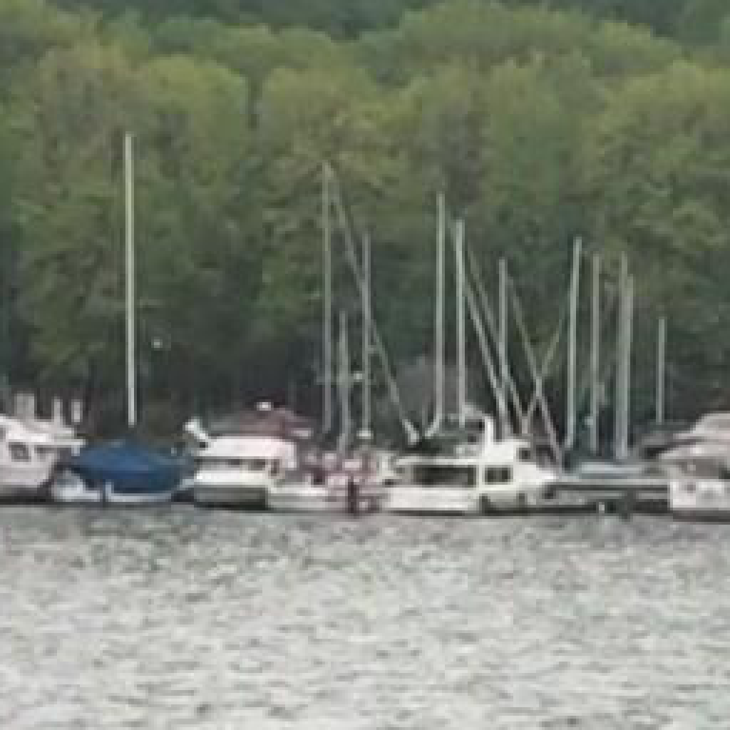
(f) gt

Figure 8: Varying training crop size. Increasing the size of training patches is a simple, yet effective method to increase image quality. Here we experiment with square patches of size $64\times 64$ 8(b) – $192\times 192$ 8(e). The visual gain is biggest for smaller patch sizes. Note how the left pole becomes sharper with increasing patch size.

We use four settings: No augmentations (other than random orientations and crops, Table 1(h)), random photometric transformations (using PyTorch’s popular random color jitter on hue, contrast, and saturation with p=0.5, Table 1(j)), random scales (with a random scale factor in $[0.25,1.0]$, Table 1(k)), and with both augmentations (Table 1(l)). We find that these augmentations significantly hurt image quality; the quantitative difference between no and both augmentations (Table 1(h vs. l)) amounts to a surprising 0.44dB. Here, the photometric augmentations alone decrease the accuracy by 0.26dB (Table 1(h vs. j)). While we do not argue that any photometric augmentation will hurt accuracy, our results suggest that the common color jitter is counterproductive in deblurring; we attribute this to the fact that commonly applied photometric co-transforms obfuscate the ground truth signal for general non-uniform blur. To illustrate this issue, let $\bm{P}$ be a photometric operator (applied to sharp images), and $\bm{K}$ be a non-uniform blur operator, respectively. If $\bm{P}$ was linear, we could derive the appropriate photometric operator $\tilde{\bm{P}}$ for blurry images as

$$\tilde{\bm{P}}\bm{K}=\bm{K}\bm{P}\quad\Rightarrow\quad\tilde{\bm{P}}=\bm{K}\bm{P}\bm{K}^{-1}.$$ (2)

As there is no ground truth $\bm{K}$ available for the GOPRO datasets, the correct photometric transformation $\tilde{\bm{P}}$ to be applied to blurry images is not available.

The performance drop induced by random scales roots in a change of relative image statistics between blurry and sharp images. To that end, consider the gradient histogram statistics of 300 training image crops shown in Fig. 4(a) as well as the statistics for rescaled crops (scale factor 0.25) in Fig. 4(b). The comparison reveals two points: First, the original statistics are sparser than the rescaled ones. Second, rescaling renders the gap of statistics between the blurry and sharp gradients less pronounced. This difference manifests in a quantitative difference of 0.22dB, c.f. Table 1(h vs. k). Visually, the difference is most apparent for blob-like regions, c.f. the leaves of the tree in Fig. 6. Not applying any photometric or scale augmentation 6(e) yields slightly clearer results than either random photometric transformations 6(b), random scales 6(c), or both 6(d).

Verdict: In contrast to other dense prediction problems, where photometric augmentations and random rescaling in training help to improve generalization, these augmentations can hurt the generalization performance of deblurring models. One should thus be careful in choosing augmentation methods, as they may obfuscate the data statistics.

Optical flow warping. Su et al. [46] experimented with pre-warping input images based on classic optical flow methods such as [39] to register them to the reference frame. Surprisingly, they did not observe any empirical benefit, hence abandoned flow warping. Yet, Chen et al. [3] use a flow network after the deblurring network to predict an output sequence of sharp images, which is subsequently registered to the reference frame. This consistency is worked into the loss function, which allows them to improve over the DBN baseline (c.f. Table 2). Kim et al. [22] propose to put a spatio-temporal transformer network in front of the DBN baseline to transform 3D inputs (the stack of blurry input images) to the reference frame; the synthesized images and the reference frame are then fed into the baseline network. In contrast to [46], they observed the temporal correspondence to improve the deblurring accuracy.

While using a spatio-temporal transformer is elegant, we argue that the underlying correspondence estimation problem is itself very hard and requires a lot of engineering to achieve high accuracy [48]. Hence, we consider pre-warping with the output from standard optical flow networks. To avoid any efficiency concerns [22], we rely on pre-trained flow networks, which obviates backpropagating through them. We experiment with two different backbones that we put in front of our baseline: FlowNet1S (denoted as f1s) [8] and PWC-Net (denoted as pwc) [47]. For both backbones, we warp the neighboring frames to the reference frame, and either input the reference frame along the replaced, warped neighbors (+ rep), or we concatenate the warped neighbors with the original input (+ cat). Note that while concatenation allows the network to possibly overcome warping artifacts using the original inputs, this is not possible without the original input. Our experiments in Table 1(m – p) show that, in contrast to the conclusions in [46], simple flow warping already helps (0.15dB improvement in (m – n) over the no-flow baseline (i)). A more substantial benefit of $\sim$0.4dB comes from concatenating the warped images along the original inputs (Table 1(o – p)). Perhaps surprisingly, the FlowNet1S backbone performs only slightly worse than PWC-Net. The visual results in Fig. 7 reveal that flow-based methods clearly improve upon the no-flow variant, which exhibits artifacts at the horizontal structures of the house. Also note how the PWC-Net backbone is clearer in deblurring the horizontal structures than the FlowNet1S variant, despite the small quantitative difference. Visually, pwc+cat further improves over pwc+rep, e.g. note the boundaries of the windows.

Table 1: Comprehensive ablation study.

#	Output activation	Initialization	Color space	Schedule	Random photom.	Random scales	Flow	Random crops	Sequence length	PSNR
a	$\operatorname{sigmoid}$	$\operatorname{fan\_out}$	RGB	short	✗	✗	-	$128^{2}$	5	$29.04$
b		$\operatorname{fan\_in}$								$29.26$
c		$\operatorname{fan\_max}$								$30.00$
d	$\operatorname{linear}$	$\operatorname{fan\_out}$	RGB	short	✗	✗	-	$128^{2}$	5	$30.09$
e		$\operatorname{fan\_in}$								$30.31$
f		$\operatorname{fan\_max}$								$31.07$
g	$\operatorname{linear}$	$\operatorname{fan\_max}$	YCbCr	short	✗	✗	-	$128^{2}$	5	$31.08$
h			RGB	long						$31.48$
i			YCbCr	long						$31.50$
j	$\operatorname{linear}$	$\operatorname{fan\_max}$	RGB	long	✓	✗	-	$128^{2}$	5	$31.22$
k					✗	✓				$31.26$
l					✓	✓				$31.04$
m	$\operatorname{linear}$	$\operatorname{fan\_max}$	RBG	long	✗	✗	f1s + rep	$128^{2}$	5	$31.62$
n							pwc + rep			$31.67$
o							f1s + cat			$31.89$
p							pwc + cat			$31.91$
q	$\operatorname{linear}$	$\operatorname{fan\_max}$	RBG	long	✗	✗	pwc + cat	$64^{2}$	5	$31.23$
r								$96^{2}$		$31.71$
s								$160^{2}$		$32.05$
t								$192^{2}$		$32.14$
u	$\operatorname{linear}$	$\operatorname{fan\_max}$	RBG	long	✗	✗	pwc + cat	$128^{2}$	7	$31.94$
v								$192^{2}$		$32.19$

Verdict: While previous work proposes a sophisticated treatment of temporal features, we find that pre-trained optical flow networks perform quite well. Concatenating warped neighbors to the inputs works significantly better than just replacing inputs. While a good flow network may not quantitatively improve over a simple one, deblurred images may show subtle improvements upon visual inspection.

Patch size and sequence length. Much of previous work [3, 22, 46, 57] is trained on random crops of size $128^{2}$, yet the significance of this choice is not further justified. In general, larger crops are beneficial as they reduce the influence of boundaries, given the typically big receptive fields. Here we explore additional patch sizes of $64^{2},96^{2},160^{2}$, and $192^{2}$, which we apply when training our pwc+cat model. Table 1(q – t) reveals that the choice of patch size – when comparing to the baseline patch size of $128^{2}$ – is quite important with a relative performance difference spanning from $-0.68$dB when using the smallest patch size $64^{2}$ to $+0.23$dB when using the largest ($192^{2}$). While the performance difference between patch sizes is more significant for smaller absolute sizes, the performance gain from very large patches is still substantial. This can also be seen in the visual results in Fig. 8. Note the clearer poles. Overall, the relative visual improvement becomes smaller with larger patch sizes, yet is still apparent.

[46] proposed to use input sequences with $5$ images, which is kept in follow up work [57, 22]. We include one more dimension in our case study, and test whether longer sequences can help. In Table 1(u–v), we increased the number of input images to $7$ and retrained our pwc+cat model (with patch sizes $128^{2}$ and $192^{2}$). The results reveal that $5$ input images largely suffice; two additional input images only yield a small benefit of $\sim 0.05$dB.

Verdict: Training patches should be chosen as big as the hardware limitations allow, since larger patch sizes provide clear benefits in accuracy. Future GPUs may allow training at full resolution and improve results further. Inputting more than $5$ images currently yields only minimal benefit.

Table 2: Deblurring performance on the GOPRO dataset of [46].

Method	PSNR	Method	PSNR
R2D+DBN [3]	$30.15$	ASL [57]	$29.10$
IFI-RNN [35]	$30.80$	DBN [46]	$30.08$
R2D+DeblurGAN [3]	$31.37$	$\text{DBN}_{128,5}$ (ours)	$31.48$
STT+DBN [22]	$31.61$	$\text{FlowDBN}_{128,5}$ (ours)	$31.91$
OVD [21, 22]	$32.28$	$\text{FlowDBN}_{192,7}$ (ours)	$32.19$
STT+OVD [22]	$32.53$

Results as reported. Results from a provided model.

4 Experiments

Evaluation on GOPRO by Su et al. [46].

As shown in the previous section, the proposed changes to Su’s baseline strikingly boosted its deblurring accuracy by over 3dB compared to our basic baseline implementation. We next consider how the improved baseline fares against the state-of-the-art. We evaluate three variants: Our best model without an optical flow backbone, trained under the same patch size ($128^{2}$) and sequence length (5) as competing methods (Table 1(h)), denoted as $\text{DBN}_{128,5}$. Our improved baseline, which includes optical flow pre-warping (Table 1(p)), denoted as $\text{FlowDBN}_{128,5}$. And our best performing model trained under large patches and two more input images (Table 1(v)), denoted as $\text{FlowDBN}_{192,7}$. Table 2 shows the quantitative evaluation on the GOPRO testing dataset of [46]. Surprisingly, even our $\text{DBN}_{128,5}$ model without optical flow already beats the highly competitive methods from Chen et al. [3] by 0.11dB, which utilizes optical flow. Our variants including optical flow, $\text{FlowDBN}_{128,5}$ and $\text{FlowDBN}_{192,7}$ are also highly competitive w.r.t. the recurrent approach of Nah et al. [35] and the spatio-temporal transformer (STT) networks [22], i.e. $\text{FlowDBN}_{128,5}$ yields a higher average PSNR than STT applied to the same DBN backbone. Finally, we improve the authors’ results of [46] by more than 2dB. While our best performing $\text{FlowDBN}_{192,7}$ cannot quite reach the accuracy of methods based on the OVD backbone [21], the OVD model exploits a dynamic temporal blending layer and uses recurrent predictions from previous iterations. In contrast, our model is based on the conceptually simpler DBN, a plain feed-forward CNN. We expect similar improvements when applying our insights in training details to the OVD backbone.

Table 3: Deblurring performance on the GOPRO dataset of [34] reported as PSNR [24] / MSSIM [53].

white[0pt][]Method

#1

#2

#3

#4

#5

#6

#7

#8

#9

#10

#11

white[][0pt]avg

white[0pt][]Reference Input

28.77/.938

27.76/.941

26.58/.881

29.83/.976

26.50/.863

23.48/.802

23.05/.820

22.83/.816

25.03/.818

23.08/.791

25.90/.894

white[][0pt]25.79/.868

white[0pt][][gray].9 DeblurGAN [26]

31.02/.968

30.37/.969

29.62/.938

31.04/.984

27.71/.906

25.41/.877

24.55/.879

25.24/.899

26.93/.891

25.64/.881

28.88/.942

white[][0pt]27.92/.922

white[0pt][]DMC [34]

31.16/.965

30.94/.971

30.57/.945

31.16/.984

28.81/.922

26.27/.898

25.38/.902

26.24/.916

27.82/.911

26.67/.907

30.62/.958

white[][0pt]28.77/.935

white[0pt][][gray].9 SRN+color [51]

32.82/.978

32.38/.980

32.21/.962

32.06/.988

29.86/.944

28.57/.946

27.81/.948

28.77/.958

29.65/.946

28.87/.948

32.71/.977

white[][0pt]30.56/.961

white[0pt][]SRN+lstm [51]

32.82/.976

32.45/.980

32.25/.961

32.12/.988

29.82/.943

28.60/.947

27.60/.946

29.03/.962

29.76/.948

28.93/.949

32.83/.978

white[][0pt]30.60/.962

white[0pt][][gray].9 $\text{DBN}_{192,1}$ (ours)

32.97/.978

32.51/.980

32.51/.964

32.17/.988

30.99/.955

28.81/.948

28.20/.955

28.88/.961

30.12/.953

29.17/.950

33.14/.978

white[][0pt]30.92/.965

white[0pt][]$\text{FlowDBN}_{128,5}$ (ours)

33.22/.982

32.71/.982

32.61/.965

32.78/.990

30.92/.955

28.78/.949

28.48/.959

28.81/.963

30.26/.954

29.03/.950

33.10/.978

white[][0pt]31.02/.966

white[0pt][][gray].9 $\text{FlowDBN}_{192,7}$ (ours)

33.56/.983

32.95/.983

33.03/.968

32.96/.991

31.32/.960

29.24/.954

28.97/.964

29.31/.968

30.66/.959

29.51/.956

33.58/.981

white[][0pt]31.42/.969

Results from a provided model.

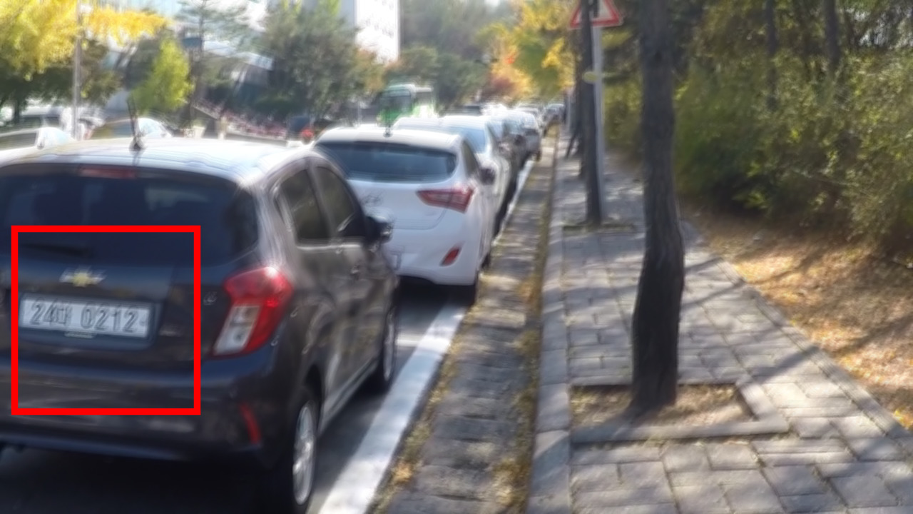
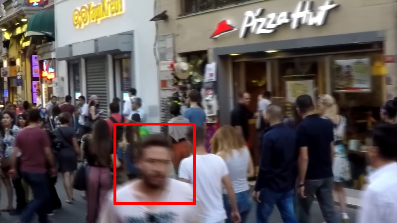
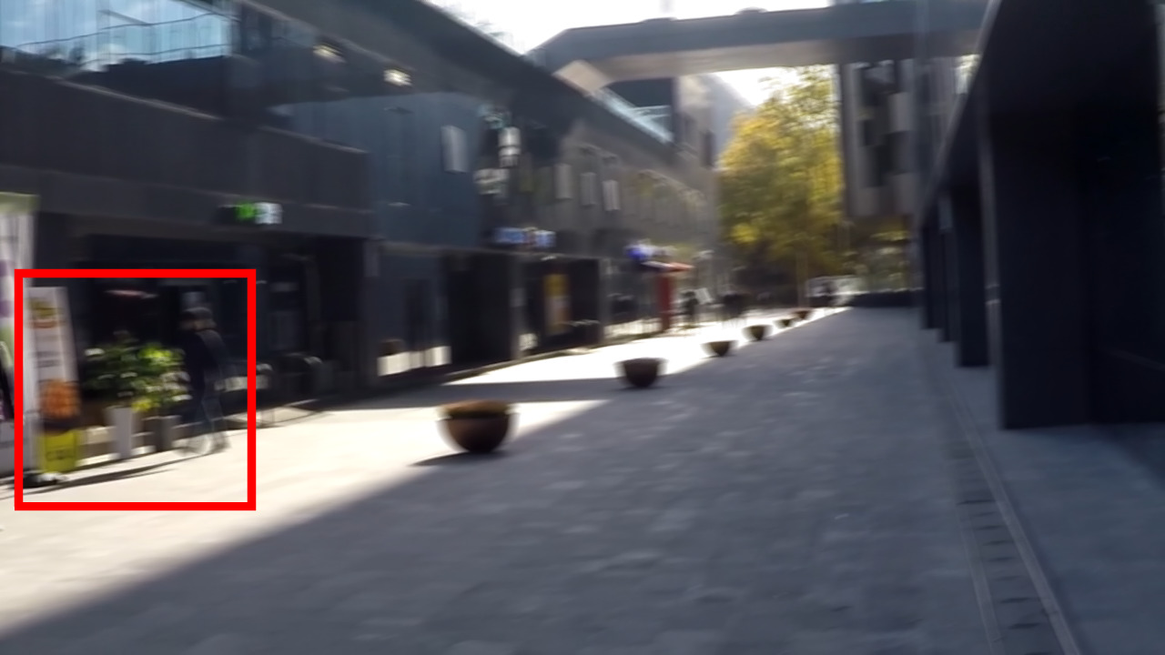
(a) Input

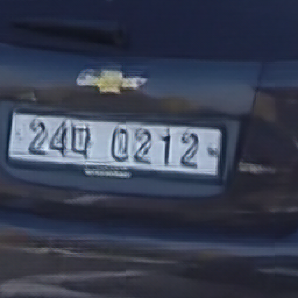
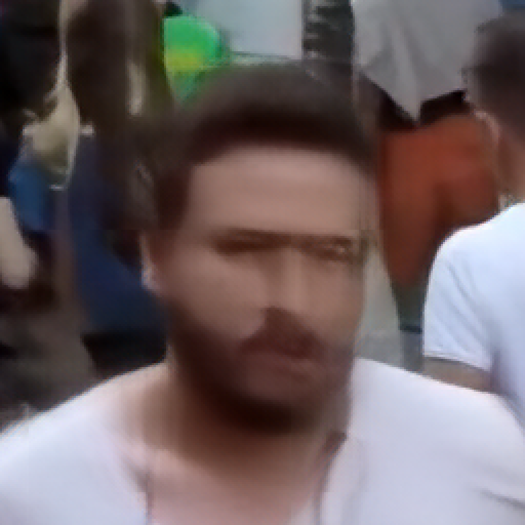
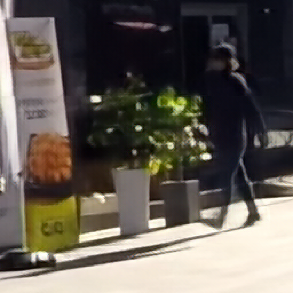
(b) DeblurGAN [26]

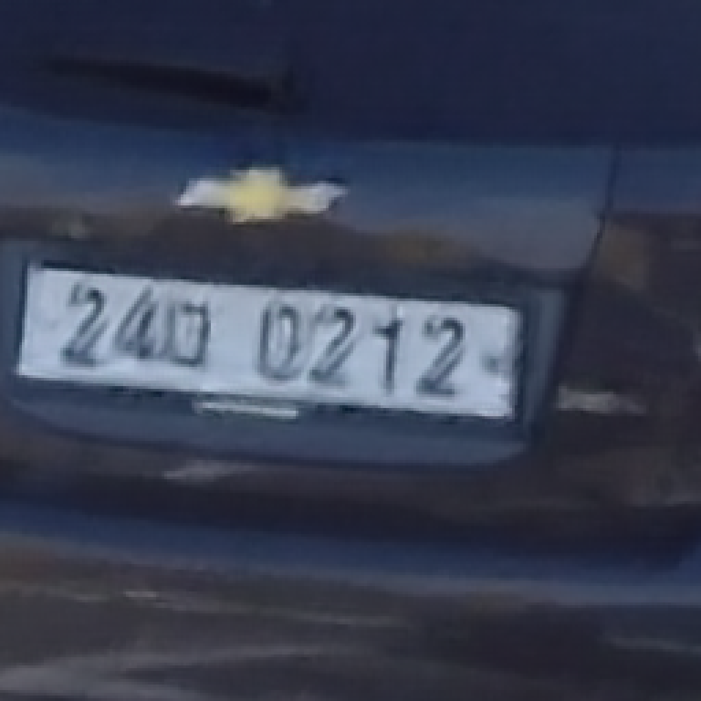
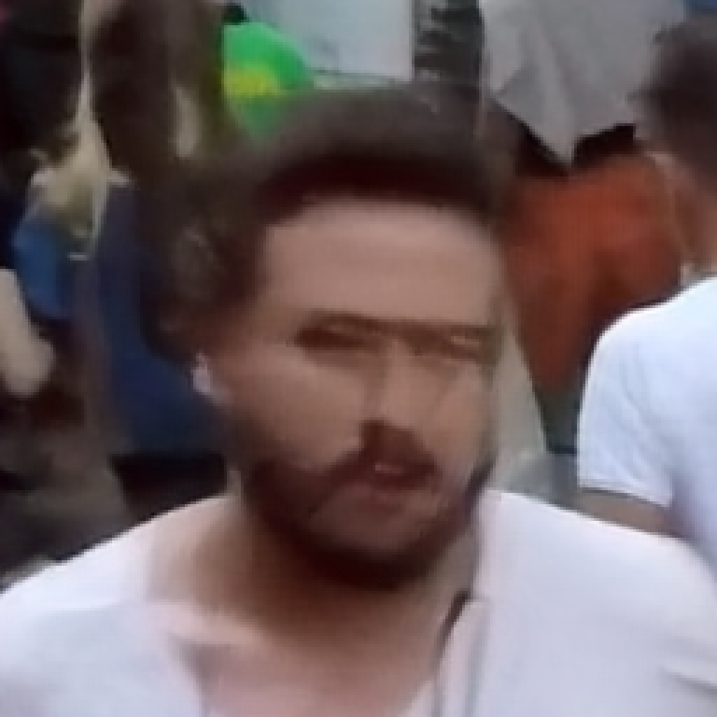
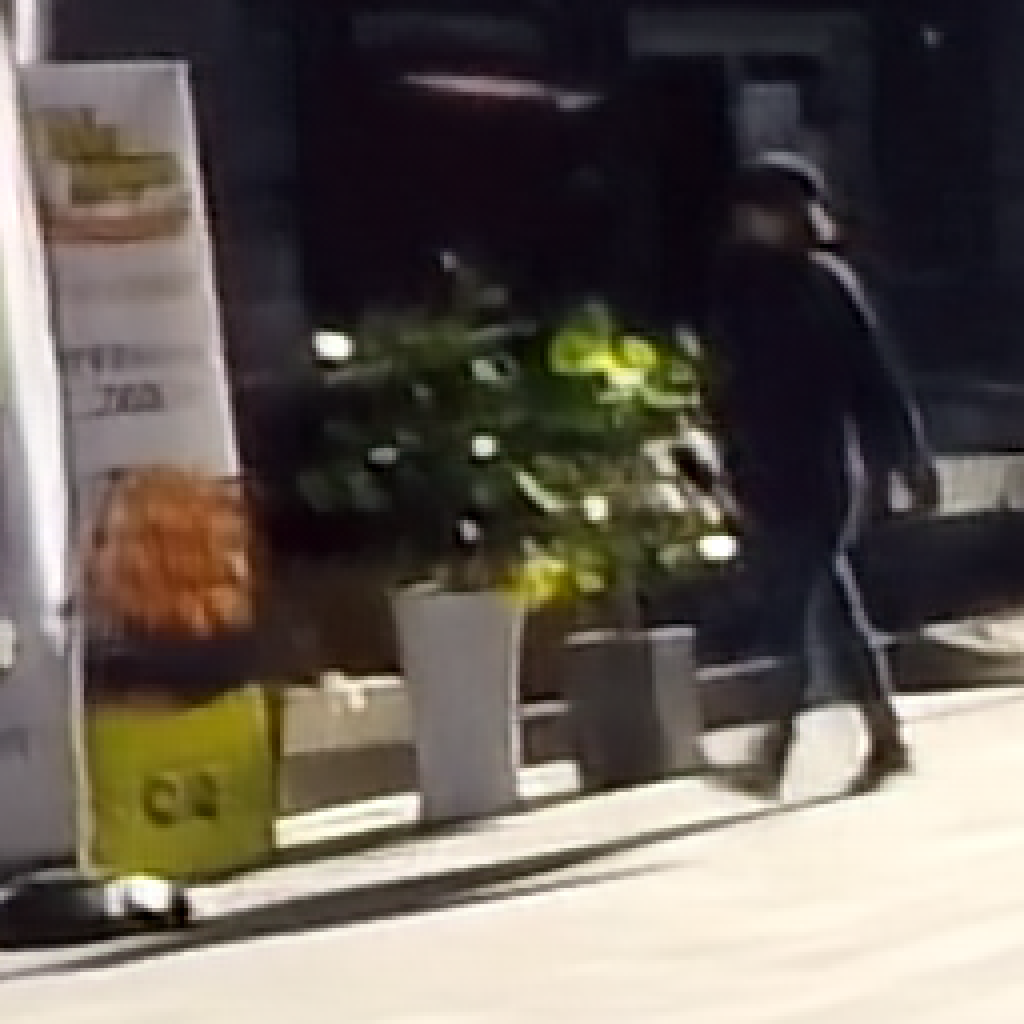
(c) DMC [34]

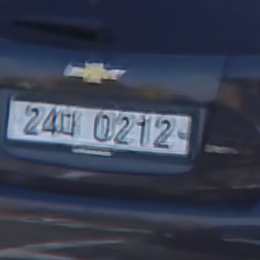
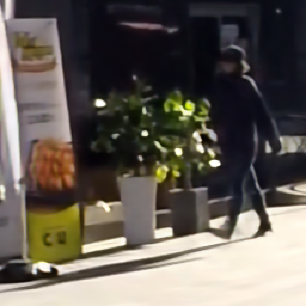
(d) SRN+lstm [51]

(e) $\text{FlowDBN}_{128,5}$

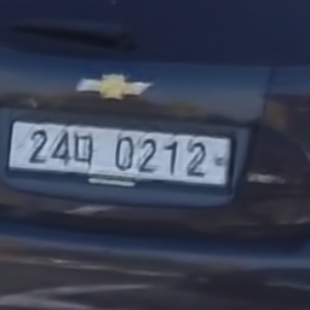
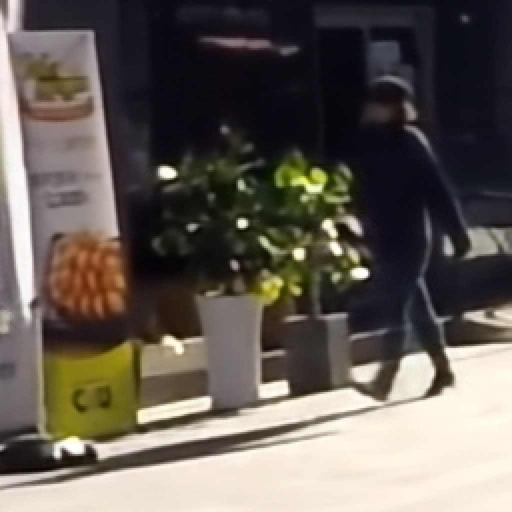
(f) $\text{FlowDBN}_{192,7}$

Figure 9: Qualitative comparison. 9(a) denotes the blurry input, 9(b) – 9(d) competing methods. Our FlowDBN models 9(e), 9(f) exhibit clearer fonts in texts (1 row), fewer artifacts for small-scale details in face deblurring (2 row), and uncover more texture from blob-like structures (orange advertisement in the 3 row).

Evaluation on GOPRO by Nah et al. [34]. To see whether the benefits we gain on our baseline generalize to other datasets, we also quantitatively evaluate on the GOPRO dataset of Nah et al. [34]. Note that the training set by [34] has roughly a third of the size of [46], hence our training schedule is three times as long, i.e. 608 epochs and halving the learning rate at epochs $[308,358,408,458,508,558]$. The other details are as described in Sec. 3.2. We compare against DeblurGAN [26], Nah et al.’s DMC baseline [34], and the two highly competitive scale-recurrent models SRN+color/lstm by Tao et al. [51]. As these methods do not exploit multiple images, we additionally include $\text{DBN}_{192,1}$, a single-image variant of our baseline.

The detailed results are shown in Table 3. Interestingly, $\text{DBN}_{192,1}$ already outperforms the highly competitive SRN+lstm model, a multiscale recurrent neural network, despite being trained on a smaller crop size (Tao et al. [51] apply $256^{2}$ crops). Both $\text{FlowDBN}_{128,5}$ and $\text{FlowDBN}_{192,7}$ perform even better, outperforming the best competing method by a very significant $\sim$0.8dB in PSNR.

Qualitative results are shown in Fig. 9. When inspecting the visual results, we find that both our FlowDBN models show perceptually better results, e.g. they exhibit clearer text deblurring (c.f. the plates in the 1 row). For moving people, faces can be problematic due to their small-scale details, as for instance shown in the results of the 2 row, i.e. DeblurGAN, DMC, and SRN+LSTM all show artifacts in the face of the person. While the results for both FlowDBN models are far from perfect, they show significantly fewer artifacts. We observe another subtle improvement in blob-like structures such as the orange repetitive structure in the advertisement (last row). Here, our FlowDBN models reconstruct a sharper texture than all competing methods.

5 Conclusion

In this paper we demonstrated how to create a highly competitive video deblurring model by revisiting details of an otherwise fairly standard CNN baseline architecture. We show that despite a lot of effort being put into finding a good video deblurring architecture by the community, some benefits could possibly be even due to seemingly minor model and training details. The resulting difference in terms of PSNR is surprisingly significant: In our study we improve the baseline network of [46] by over 2dB compared to the original results in the paper, and 3.15dB over our initial implementation, which allows this simple network to outperform more recent and much more complex models. This poses the question whether existing experimental comparisons in the deblurring literature actually uncover systematic accuracy differences from the architecture, or whether the differences may be down to detail engineering. Future work thus needs to shed more light on this important point.

References

- [1] Ayan Chakrabarti. A neural approach to blind motion deblurring. In ECCV, volume 3, pages 221–235, 2016.
- [2] Ken Chatfield, Karen Simonyan, Andrea Vedaldi, and Andrew Zisserman. Return of the devil in the details: Delving deep into convolutional nets. In BMVC, 2014.
- [3] Huaijin Chen, Jinwei Gu, Orazio Gallo, Ming-Yu Liu, Ashok Veeraraghavan, and Jan Kautz. Reblur2Deblur: Deblurring videos via self-supervised learning. In ICCP, 2018.
- [4] Sunghyun Cho and Seungyong Lee. Fast motion deblurring. ACM T. Graphics, 28(5):145:1–145:8, Dec. 2009.
- [5] Sunghyun Cho, Jue Wang, and Seungyong Lee. Video deblurring for hand-held cameras using patch-based synthesis. ACM T. Graphics, 31(4):64:1–64:9, July 2012.
- [6] Florent Couzinié-Devy, Jian Sun, Karteek Alahari, and Jean Ponce. Learning to estimate and remove non-uniform image blur. In CVPR, pages 1075–1082, 2013.
- [7] Mauricio Delbracio and Guillermo Sapiro. Hand-held video deblurring via efficient Fourier aggregation. IEEE T. Comput. Imag., 1(4):270–283, Dec. 2015.
- [8] Alexey Dosovitskiy, Philipp Fischer, Eddy Ilg, Philip Häusser, Caner Hazırbaş, Vladimir Golkov, Patrick van der Smagt, Daniel Cremers, and Thomas Brox. FlowNet: Learning optical flow with convolutional networks. In ICCV, pages 2758–2766, 2015.
- [9] Rob Fergus, Barun Singh, Aaron Hertzmann, Sam T. Roweis, and William T. Freeman. Removing camera shake from a single photograph. ACM T. Graphics, 25(3):787–794, July 2006.
- [10] Jochen Gast, Anita Sellent, and Stefan Roth. Parametric object motion from blur. In CVPR, pages 1846–1854, 2016.
- [11] Dong Gong, Jie Yang, Lingqiao Liu, Yanning Zhang, Ian Reid, Chunhua Shen, Anton van den Hengel, and Qinfeng Shi. From motion blur to motion flow: A deep learning solution for removing heterogeneous motion blur. In CVPR, pages 3806–3815, 2017.
- [12] Ankit Gupta, Neel Joshi, C. Lawrence Zitnick, Michael Cohen, and Brian Curless. Single image deblurring using motion density functions. In ECCV, volume 1, pages 171–184, 2010.
- [13] Kaiming He, Xiangyu Zhang, Shaoqing Ren, and Jian Sun. Delving deep into rectifiers: Surpassing human-level performance on ImageNet classification. In ICCV, pages 1026–1034, 2015.
- [14] Michael Hirsch, Christian J. Schuler, Stefan Harmeling, and Bernhard Schölkopf. Fast removal of non-uniform camera shake. In ICCV, pages 463–470, 2011.
- [15] Eddy Ilg, Nikolaus Mayer, Tonmoy Saikia, Margret Keuper, Alexey Dosovitskiy, and Thomas Brox. FlowNet 2.0: Evolution of optical flow estimation with deep networks. In CVPR, pages 1647–1655, 2017.
- [16] Sergey Ioffe and Christian Szegedy. Batch normalization: Accelerating deep network training by reducing internal covariate shift. In ICML, pages 448–456, 2015.
- [17] Meiguang Jin, Stefan Roth, and Paolo Favaro. Normalized blind deconvolution. In ECCV, volume 7, pages 694–711, 2018.
- [18] Tae Hyun Kim, Byeongjoo Ahn, and Kyoung Mu Lee. Dynamic scene deblurring. In ICCV, pages 3160–3167, 2013.
- [19] Tae Hyun Kim and Kyoung Mu Lee. Segmentation-free dynamic scene deblurring. In CVPR, pages 2766–2773, 2014.
- [20] Tae Hyun Kim and Kyoung Mu Lee. Generalized video deblurring for dynamic scenes. In CVPR, pages 5426–5434, 2015.
- [21] Tae Hyun Kim, Kyoung Mu Lee, Bernhard Schölkopf, and Michael Hirsch. Online video deblurring via dynamic temporal blending network. In ICCV, pages 4058–4067, 2017.
- [22] Tae Hyun Kim, Mehdi S. M. Sajjadi, Michael Hirsch, and Bernhard Schölkopf. Spatio-temporal transformer network for video restoration. In ECCV, volume 3, pages 111–127, 2018.
- [23] Diederik P. Kingma and Jimmy Lei Ba. Adam: A method for stochastic optimization. In ICLR, 2015.
- [24] Rolf Köhler, Michael Hirsch, Betty Mohler, Bernhard Schölkopf, and Stefan Harmeling. Recording and playback of camera shake: Benchmarking blind deconvolution with a real-world database. In ECCV, volume 7, pages 27–40, 2012.
- [25] Dilip Krishnan, Terence Tay, and Rob Fergus. Blind deconvolution using a normalized sparsity measure. In CVPR, pages 233–240, 2011.
- [26] Orest Kupyn, Volodymyr Budzan, Mykola Mykhailych, Dmytro Mishkin, and Jiři Matas. DeblurGAN: Blind motion deblurring using conditional adversarial networks. In CVPR, pages 8183–8192, 2018.
- [27] Anat Levin. Blind motion deblurring using image statistics. In NIPS*2006, pages 841–848.
- [28] Anat Levin, Yair Weiss, Fredo Durand, and William T. Freeman. Understanding and evaluating blind deconvolution algorithms. In CVPR, pages 1964–1971, 2009.
- [29] Anat Levin, Yair Weiss, Fredo Durand, and William T. Freeman. Efficient marginal likelihood optimization in blind deconvolution. In CVPR, pages 2657–2664, 2011.
- [30] Mario Lucic, Karol Kurach, Marcin Michalski, Olivier Bousquet, and Sylvain Gelly. Are GANs created equal? A large-scale study. In NeurIPS*2018, pages 700–709.
- [31] Yasuyuki Matsushita, Eyal Ofek, Weina Ge, Xiaoou Tang, and Heung-Yeung Shum. Full-frame video stabilization with motion inpainting. IEEE T. Pattern Anal. Mach. Intell., 28(7):1150–1163, July 2006.
- [32] Tomer Michaeli and Michal Irani. Blind deblurring using internal patch recurrence. In ECCV, volume 3, pages 783–798, 2014.
- [33] James Miskin and David J. C. MacKay. Ensemble learning for blind image separation and deconvolution. In Mark Girolami, editor, Advances in Independent Component Analysis, Perspectives in Neural Computing, chapter 7, pages 123–141. Springer London, 2000.
- [34] Seungjun Nah, Tae Hyun Kim, and Kyoung Mu Lee. Deep multi-scale convolutional neural network for dynamic scene deblurring. In CVPR, pages 257–265, 2017.
- [35] Seungjun Nah, Sanghyun Son, and Kyoung Mu Lee. Recurrent neural networks with intra-frame iterations for video deblurring. In CVPR, pages 8102–8111, 2019.
- [36] Mehdi Noroozi, Paramanand Chandramouli, and Paolo Favaro. Motion deblurring in the wild. In GCPR, pages 65–77, 2017.
- [37] Jinshan Pan, Deqing Sun, Hanspeter Pfister, and Ming-Hsuan Yang. Blind image deblurring using dark channel prior. In CVPR, pages 1628–1636, 2016.
- [38] Razvan Pascanu, Tomas Mikolov, and Yoshua Bengio. On the difficulty of training recurrent neural networks. In ICML, pages 1310–1318, 2013.
- [39] Javier Sánchez Pérez, Enric Meinhardt-Llopis, and Gabriele Facciolo. TV-L1 optical flow estimation. Image Process. On Line, 3:137–150, 2013.
- [40] Daniele Perrone and Paolo Favaro. Total variation blind deconvolution: The devil is in the details. In CVPR, pages 2909–2916, 2014.
- [41] Sainandan Ramakrishnan, Shubham Pachori, Aalok Gangopadhyay, and Shanmuganathan Raman. Deep generative filter for motion deblurring. In ICCV Workshops, pages 2993–3000, 2017.
- [42] Wenqi Ren, Jinshan Pan, Xiaochun Cao, and Ming-Hsuan Yang. Video deblurring via semantic segmentation and pixel-wise non-linear kernel. In ICCV, pages 1086–1094, 2017.
- [43] Kevin Schelten, Sebastian Nowozin, Jeremy Jancsary, Carsten Rother, and Stefan Roth. Interleaved regression tree field cascades for blind image deconvolution. In WACV, pages 494–501, 2015.
- [44] Christian J. Schuler, Michael Hirsch, Stefan Harmeling, and Bernhard Schölkopf. Learning to deblur. IEEE T. Pattern Anal. Mach. Intell., 38(7):1439–1451, July 2016.
- [45] Qi Shan, Jiaya Jia, and Aseem Agarwala. High-quality motion deblurring from a single image. ACM T. Graphics, 27(3):73:1–73:10, Aug. 2008.
- [46] Shuochen Su, Mauricio Delbracio, Jue Wang, Guillermo Sapiro, Wolfgang Heidrich, and Oliver Wang. Deep video deblurring for hand-held cameras. In CVPR, pages 237–246, 2017.
- [47] Deqing Sun, Xiaodong Yang, Ming-Yu Liu, and Jan Kautz. PWC-Net: CNNs for optical flow using pyramid, warping, and cost volume. In CVPR, pages 8934–8943, 2018.
- [48] Deqing Sun, Xiaodong Yang, Ming-Yu Liu, and Jan Kautz. Models matter, so does training: An empirical study of CNNs for optical flow estimation. IEEE T. Pattern Anal. Mach. Intell., 2019, to appear.
- [49] Jian Sun, Wenfei Cao, Zongben Xu, and Jean Ponce. Learning a convolutional neural network for non-uniform motion blur removal. In CVPR, pages 769–777, 2015.
- [50] Libin Sun, Sunghyun Cho, Jue Wang, and James Hays. Edge-based blur kernel estimation using patch priors. In ICCP, 2013.
- [51] Xin Tao, Hongyun Gao, Xiaoyong Shen, Jue Wang, and Jiaya Jia. Scale-recurrent network for deep image deblurring. In CVPR, pages 8174–8182, 2018.
- [52] Xintao Wang, Kelvin C. K. Chan, Ke Yu, Chao Dong, and Chen Change Loy. EDVR: Video restoration with enhanced deformable convolutional networks. In CVPR Workshops, 2019.
- [53] Zhou Wang, Eero P. Simoncelli, and Alan C. Bovik. Multi-scale structural similarity for image quality assessment. In ACSSC, pages 1398–1402, 2003.
- [54] Oliver Whyte, Josef Sivic, Andrew Zisserman, and Jean Ponce. Non-uniform deblurring for shaken images. In CVPR, pages 491–498, 2010.
- [55] Li Xu and Jiaya Jia. Two-phase kernel estimation for robust motion deblurring. In ECCV, volume 1, pages 157–170, 2010.
- [56] Li Xu, Shicheng Zheng, and Jiaya Jia. Unnatural sparse representation for natural image deblurring. In CVPR, pages 1107–1114, 2013.
- [57] Kaihao Zhang, Wenhan Luo, Yiran Zhong, Lin Ma, Wei Liu, and Hongdong Li. Adversarial spatio-temporal learning for video deblurring. IEEE T. Image Process., 28(1):291–301, Jan. 2019.
- [58] Shicheng Zheng, Li Xu, and Jiaya Jia. Forward motion deblurring. In ICCV, pages 1465–1472, 2013.