How hard is it to predict sandpiles on lattices? A survey.

Abstract

Since their introduction in the 80s, sandpile models have raised interest for their simple definition and their surprising dynamical properties. In this survey we focus on the computational complexity of the prediction problem, namely, the complexity of knowing, given a finite configuration $c$ and a cell $x$ in $c$, if cell $x$ will eventually become unstable. This is an attempt to formalize the intuitive notion of “behavioral complexity” that one easily observes in simulations. However, despite many efforts and nice results, the original question remains open: how hard is it to predict the two-dimensional sandpile model of Bak, Tang and Wiesenfeld?

1 Introduction

Langton proposed to describe complex dynamical systems as being at the “edge of chaos” [44]. Complexity arises in a context that is neither too ordered, i.e. not exhibiting a rigid structure allowing to efficiently understand and predict the future state of the system, nor completely chaotic, i.e. avoiding pseudo-random behaviour and uncomputable long-term effects. From a computer science point of view, complex dynamical systems are an object of great interest because they precisely model physical systems that are able to perform non-trivial computation.

In 1990, Moore et. al. started to formalize the intuitive notion of “complexity” of a system, through the computational complexity of predicting the behaviour of the system [41, 48, 49, 50, 55, 56] (for other kinds of complexity in dynamical systems, see for instance [17, 18, 20, 1, 16, 11, 10, 19]). Computational complexity theory is actually a perfect fit to capture the complexity of systems able to compute. In turned out that the hierarchy of complexity classes offers a very precise way to characterize the behavioural complexity of discrete dynamical systems. For example if a system has a ${\mathsf{P}}$-hard prediction problem, it means that it is able to efficiently simulate a general purpose sequential computer (such as a Turing machine), whereas if the prediction problem is much below in the hierarchy, let say in ${\mathsf{L}}$, then the system can only compute under severe space restriction, and therefore cannot perform efficiently any computation if we assume ${\mathsf{P}}\neq{\mathsf{L}}$. In this precise sense the former would be more complex than the latter.

At the same time, the sandpile model of Bak, Tang and Wiesenfeld [2, 3] gained interest. It exhibits both a “complex” behaviour and a very elegant algebraic structure [22]. Unsurprisingly, sandpile models are capable of universal computation [34]. In 1999, Moore and Nilsson began to apply the computational complexity vocabulary to capture the intuitive “complexity” of sandpile models [54]. Moreover, they observed a dimension sensitivity that received great attention. It is the purpose of this survey to review such very interesting results and to generalise some of them.

Sandpile models are a subclass of number-conserving cellular automata where we are given a $d$-dimensional lattice ($\mathbb{Z}^{d}$) with a finite amount of sand grains at each cell. A local rule applied in parallel at every cell let grains topple: if the sand content at a cell is greater or equal to $2d$, then the cell gives one grain to each of the $2d$ cells it touches (two cells in each dimension). This is the very first sandpile model of Bak, Tang and Wiesenfeld, which they defined for $d=2$. This is also the sandpile model studied by Moore and Nilsson, for which they proved the following foundations.

• In dimension one it is possible to predict efficiently the dynamics with a parallel algorithm (complexity class ${\mathsf{NC}}$).

• In dimension three or more it is not possible to predict efficiently the dynamics with a parallel algorithm, unless some classical complexity conjecture is wrong (unless ${\mathsf{P}}={\mathsf{NC}}$, since prediction is proven to be a ${\mathsf{P}}$-hard problem). In other terms, in this case the dynamics is inherently sequential.

This survey concentrates on lattice $\mathbb{Z}^{d}$, because of this interest in the dimension sensitivity. In a more general setting than lattices, sandpiles can very easily embed arbitrary computation and become almost always hard to predict from a computational complexity point of view [35].

Sandpile models have close relatives, the family of majority cellular automata. Indeed, though the latter model is not number-conserving, open questions on its two-dimensional prediction are remarkably similar [53]. Goles et. al. made progress in various directions to capture the essence of ${\mathsf{P}}$-completeness in majority cellular automata [33, 36, 37, 38, 39], with notable applications of ${\mathsf{NC}}$ algorithms from [43]. Cellular automata with finite support are very close to sandpiles when considered under the sequential update policy. However, in this context we witness a general increase of the complexity of the (decidable) questions about the dynamics which seems not to happen in sandpiles [18].

The paper is structured as follows. In Section 2 we define sandpile models on lattices with uniform neighborhood, formulate three versions of the prediction problem, introduce some classical considerations, and briefly review the complexity classes at stake. Subsequent sections survey known results, and generalise some of them or propose conjectures. All prediction problems are in ${\mathsf{P}}$ (Section 3). The dimension sensitivity for arbitrary sandpile models generalizes as follows: in dimension one prediction is in ${\mathsf{NC}}$ (Section 4), in dimension three or above it is ${\mathsf{P}}$-complete (Section 5), and in two dimensions the precise complexity classification remains open for the original sandpile model with von Neumann neighborhood, though insightful results have been obtained around this question (Section 6). Finally, we briefly mention how undecidability may arise when the finiteness condition on the initial configuration is relaxed (Section 8).

2 Definitions

Since their introduction by Bak, Tang and Wiesenfeld in [2], sandpiles underwent many generalizations. In this survey we propose a general framework which tries to cover all such models. However, we will focus only over lattices of arbitrary dimension and uniform (in space and time) number-conserving local rules. This section includes formalization of folklore terminology and considerations extended to this general setting.

2.1 Sandpile models on lattices with uniform neighborhood

Let $\mathbb{N}_{+}$ (resp. $\mathbb{N}_{-}$) denote the set of strictly positive (resp. negative) integers. For any dimension $d\in\mathbb{N}_{+}$, a cell is a point in $\mathbb{Z}^{d}$. A configuration is an assignment of a finite number of sand grains to each cell i.e. it is an element of $\mathbb{N}^{\mathbb{Z}^{d}}$. A sandpile model is a structure $\left\langle\mathcal{N},\mathcal{D},\theta\right\rangle$ where $\mathcal{N}$ is a finite subset of $\mathbb{Z}^{d}\setminus\{0^{d}\}$ called neighborhood and $\mathcal{D}\in{\mathbb{N}_{+}}^{\mathcal{N}}$ is distribution of sand grains w.r.t. the neighborhood $\mathcal{N}$ (it is required that ${\mathsf{dom}}(\mathcal{D})=\mathcal{N}$) and $\theta=\sum_{x\in\mathcal{N}}\mathcal{D}(x)$ is the stability threshold. To avoid irrelevant technicalities, we will consider only complete neighborhoods $\mathcal{N}$, that is to say such that

$${\mathsf{span}^{+}}(\mathcal{N})=\mathbb{Z}^{d},$$ (1)

where ${\mathsf{span}^{+}}(\mathcal{N})$ is the set of positive integer linear combinations of cell coordinates from $\mathcal{N}$. Moreover, remark that, for simplicity sake, we assumed that $0^{d}\notin\mathcal{N}$ i.e. cells do not belong to their own neighborhoods. Indeed, allowing $0^{d}\in\mathcal{N}$ would only correspond to having irremovable grains in each cell.

The dynamics associated with a sandpile model is the parallel application of the following local rule: if a cell has at least $\theta$ grains, then it redistributes $\theta$ of its grains to its neighborhood $x+\mathcal{N}$, according to the distribution $\mathcal{D}$. More formally, denote $F:\mathbb{N}^{\mathbb{Z}^{d}}\to\mathbb{N}^{\mathbb{Z}^{d}}$ the global rule which associates any configuration $c\in\mathbb{N}^{\mathbb{Z}^{d}}$ with a configuration $F(c)\in\mathbb{N}^{\mathbb{Z}^{d}}$ defined as follows

$$\forall x\in\mathbb{Z}^{d}:\big{(}F(c)\big{)}(x)=c(x)-\theta\mathsf{H}\left(c(x)-\theta\right)+\sum_{y\in\mathcal{N}}\mathcal{D}(y)\mathsf{H}\left(c(x+y)-\theta\right)$$ (2)

where $\mathsf{H}\left(n\right)$ equals $1$ if $n\geq 0$, and equals $0$ otherwise (the classical Heaviside function). From the Equation (2), it is clear that the knowledge of the distribution $\mathcal{D}$ suffices to completely specify the dynamics since from the domain of $\mathcal{D}$ one can deduce $\mathcal{N}$ and the dimension $d$, and from $\mathcal{D}$ one finds $\theta$. However, we shall prefer to provide explicitly $\left\langle\mathcal{N},\mathcal{D},\theta\right\rangle$, at least in this introductory material.

The system characterized by Equation (2) is number-conserving in the sense the total number of sand grains is conserved along its evolution as stated in the following.

Proposition 1 (Number conservation).

For any configuration $c\in\mathbb{N}_{+}^{\mathbb{Z}^{d}}$, it holds

$$\#(F(c))=\#(c)$$

where $\#(c)=\sum_{x\in\mathbb{Z}^{d}}c(x)$. Note that $\#(c)$ could be positive infinity.

Figure 1 provides an illustration of a simple sandpile model and its dynamics.

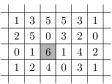
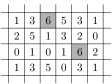
          $\overset{F}{\mapsto}$ $\overset{F}{\mapsto}$

Figure 1: An example of sandpile model neighborhood and distribution (left, $\theta=6$), and two steps of the global rule from a finite configuration (right, outside the pictured region the configuration is considered as initially empty). Unstable cells are marked. Only the interesting portion of the configuration is drawn.

Remark 1.

In this general framework, the Moore sandpile model of dimension $d$ and radius $r$ corresponds to $\left\langle\mathcal{N}_{\text{M}},\mathcal{D}_{1},(2r+1)^{d}-1\right\rangle$ where $\mathcal{N}_{\text{M}}={\left\{-r,\ldots,r\right\}}^{d}\setminus{\left\{0^{d}\right\}}$ and $\mathcal{D}_{1}$ is the constant function equal to $1$ for any element of its domain. The von Neumann sandpile model of dimension $d$ and radius $r$ corresponds to $\left\langle\mathcal{N}_{\text{VN}},\mathcal{D}_{1},2rd\right\rangle$ where

$$\mathcal{N}_{\text{VN}}={\left\{(x_{1},\ldots,x_{d})\in{\left\{-r,\ldots,r\right\}}^{d}\,\mid\,\exists i:(x_{i}\neq 0\text{ and }\forall j\neq i:x_{j}=0)\right\}}\enspace$$

(this is the original model of Bak, Tang and Wiesenfeld [2] for $d=2$ and $r=1$).

Denote $c\to c^{\prime}$ whenever $c^{\prime}=F(c)$, and let $\stackrel{{\scriptstyle*}}{{\to}}$ be the reflexive and transitive closure of $\to$. Given a cell $x$, remark that its neighbors might play different roles. Indeed, one can distinguish the out-neighbors of $x$ as the set of cells $x+\mathcal{N}=\{y\mid(y-x)\in\mathcal{N}\}$ from the in-neighbors which are $x-\mathcal{N}=\{y\mid(x-y)\in\mathcal{N}\}$.

Remark 2.

Another even more general way to define sandpile models is on an arbitrary multi-digraph $G=(V,A)$ (where $A$ is a multiset), where each vertex has finite in-degree and finite out-degree. In this case, configurations $c$ are taken in $\mathbb{N}^{V}$ and the local rule would be: if $v\in V$ contains at least $d^{+}(v)$ grains ($d^{+}(v)$ is the out-degree of node $v$) then it gives one grain along each of its out-going arcs. When the graph supporting the dynamics is not a lattice, sandpile models are also called chip firing games in the literature [6, 7].

A cell $x$ is stable if $c(x)<\theta$, and unstable otherwise. A configuration is stable when all cells are stable, and is unstable if at least one cell is unstable. Remark that stable configurations are fixed points of the global rule $F$. From the Equation (2), it is clear that the system is deterministic and therefore given a configuration $c$ and a stable configuration $c^{\prime}$ either there is a unique sequence of configurations $c=c_{1}\to c_{2}\to\dots\to c_{n}=c^{\prime}$ or $c\not\stackrel{{\scriptstyle*}}{{\to}}c^{\prime}$. However, one can consider also other types updating policies. The sequential policy consists in choosing non-deterministically a cell from the unstable ones and in updating only this chosen cell. Then, repeat the same update policy on the newly obtained configuration and so on. It is clear that the new dynamics might be very different from the one obtained from Equation (2). Sandpiles models in which the sequential update and the parallel update policies produce the same set of stable configurations with the same number of topplings are called Abelian. Recall that the terms firing and toppling are employed to describe the action of moving sand grains from unstable cells to other cells. The stabilization of a configuration $c$ is the process of reaching a stable configuration. A finite configuration contains a finite number of grains, or equivalently its number of non-empty cells is finite.

The topplings counter, usually called shot vector or odometer function in the literature, started at an initial configuration configuration $c$ is a very useful formal tool for the analysis of sandpiles and it is defined as follows. For all configurations $c,c^{\prime},c^{\prime\prime}$ if $c\to c^{\prime}$ then,

$$\forall x\in\mathbb{Z}^{d}:{\mathsf{odo}}(c,c^{\prime})(x)=\mathsf{H}\left(c(x)-\theta\right),$$

and if $c\stackrel{{\scriptstyle*}}{{\to}}c^{\prime}\to c^{\prime\prime}$ then

$$\forall x\in\mathbb{Z}^{d}:{\mathsf{odo}}(c,c^{\prime\prime})(x)={\mathsf{odo}}(c,c^{\prime})(x)+{\mathsf{odo}}(c^{\prime},c^{\prime\prime})(x)$$

with the convention ${\mathsf{odo}}(c,c)(x)=0$ for all $x\in\mathbb{Z}^{d}$.

Let $c\stackrel{{\scriptstyle x}}{{\rightharpoonup}}c^{\prime}$ denote application of the sequential update policy at cell $x$ i.e., one has $c\stackrel{{\scriptstyle x}}{{\rightharpoonup}}c^{\prime}$ if and only if

$$c^{\prime}(y)=\left\{\begin{array}[]{ll}c(y)-\theta\,\mathsf{H}\left(c(y)-\theta\right)&\text{ if }y=x\\ c(y)+\mathcal{D}(y-x)\,\mathsf{H}\left(c(x)-\theta\right)&\text{ if }y\in x+\mathcal{N}\\ c(y)&\text{ otherwise.}\end{array}\right.$$

We also simply denote $c\stackrel{{\scriptstyle}}{{\rightharpoonup}}c^{\prime}$ when there exists $x$ such that $c\stackrel{{\scriptstyle x}}{{\rightharpoonup}}c^{\prime}$. Moreover, let $\stackrel{{\scriptstyle*}}{{\rightharpoonup}}$ denote the reflexive transitive closure of $\stackrel{{\scriptstyle}}{{\rightharpoonup}}$, and ${\mathsf{odo}_{\rightharpoonup}}(c,c^{\prime})$ denote the odometer function under the sequential update policy (it counts the number of topplings occurring at each cell to reach $c^{\prime}$ from $c$). The Abelian property can be formally stated as follows.

Proposition 2.

For any sandpile model, given a configuration $c$, if $c\to c^{\prime}$ then $c\stackrel{{\scriptstyle*}}{{\rightharpoonup}}c^{\prime}$.
Moreover, if $c\stackrel{{\scriptstyle*}}{{\to}}c^{\prime}$ and $c^{\prime}$ is a stable configuration, then

1. $c\stackrel{{\scriptstyle*}}{{\rightharpoonup}}c^{\prime}$,

2. $c\not\stackrel{{\scriptstyle*}}{{\rightharpoonup}}c^{\prime\prime}$ for any other stable configuration $c^{\prime\prime}$,

3. ${\mathsf{odo}}(c,c^{\prime})={\mathsf{odo}_{\rightharpoonup}}(c,c^{\prime})$.

We stress that Proposition 2 is an important feature in our context. Indeed, it states that the (non-deterministic) sequential policy always leads to the same stable configuration as the parallel policy, with exactly the same number of topplings at each cell. Relaxing this requirement deeply changes the dynamics and the structure of the phase space (it has no more a lattice structure for example). For non-abelian models see for example [30, 27].

Endowing the set of configurations with binary addition $+$ (given two configurations $c,c^{\prime}$, $(c+c^{\prime})(x)=c(x)+c^{\prime}(x)$ for all $x$ i.e. grain content is added cell-wise), $\mathbb{N}^{\mathbb{Z}^{d}}$ is a commutative monoid. It is also the case of the set of stable configurations, where the addition is defined as addition followed by stabilization. The famous Abelian sandpile group of recurrent configurations appears when a global sink is added to the multi-digraph supporting the dynamics. This subject goes beyond the scope of the present survey, for more see [24, 23].

2.2 Prediction problems

Given a sandpile model $\left\langle\mathcal{N},\mathcal{D},\theta\right\rangle$, the basic prediction problem asks if a certain cell $x$ will become unstable when the system is started from a given finite initial configuration $c$. More formally,

Prediction problem ($\mathsf{PRED}$).
Input: a finite configuration $c\in\mathbb{N}^{\mathbb{Z}^{d}}$ and a cell $x\in\mathbb{Z}^{d}$. Question: will cell $x$ eventually become unstable during the evolution from $c$?

One of the most intriguing features of sandpiles is that they are a paradigmatic example of self-organized criticality. Indeed, starting from an initial configuration and adding grains at random positions, the system reaches a stable configuration $c$ from which a small perturbation (an addition of a single grain at some cell) may trigger an arbitrarily large chain of reactions commonly called an avalanche. The distribution of sizes of avalanches (when grains are added at random) follow a power law . We are interested in the computational complexity of deciding if a given cell $x$ will topple during this process. More formally, one can ask the following.

Stable prediction problem ($\mathsf{S\text{-}PRED}$).
Input: a stable finite configuration $c\in\mathbb{N}^{\mathbb{Z}^{d}}$, two cells $x,y\in\mathbb{Z}^{d}$. Question: does adding one grain on cell $y$ from $c$ trigger a chain of reactions that will eventually make $x$ become unstable?

A variant of $\mathsf{S\text{-}PRED}$ is obtained when the cell $y$ is fixed from the very beginning. When $y$ is the lexicographically minimal cell (i.e. the cell of the finite configuration with the lexicographically minimal coordinates), one has the following.

First column stable prediction problem ($\mathsf{1^{\text{st}}col\text{-}S\text{-}PRED}$).
Input: a stable finite configuration $c\in\mathbb{N}^{\mathbb{Z}^{d}}$ and a cell $x\in\mathbb{Z}^{d}$. Question: does adding one grain on the (lexicographically) minimal cell of $c$ trigger a chain of reactions that will eventually make $x$ become unstable?

Adding the grain at an extremity of the configuration (the lexicographically minimal cell) implies a strong monotonicity of the dynamics, which has been especially useful in one-dimensional proofs of ${\mathsf{NC}}$ness (see Subection 2.3 and Proposition 4)). $\mathsf{1^{\text{st}}col\text{-}S\text{-}PRED}$ has also been called the Avalanche problem.

Finally, one can simply ask how hard it is to compute the stable configuration reached when starting from a given finite initial configuration. In other words,

Computational prediction problem ($\mathsf{Compute\text{-}PRED}$).
Input: a finite configuration $c\in\mathbb{N}^{\mathbb{Z}^{d}}$. Output: what is the stable configuration reached when starting at $c$?

Before stepping to the detailed study of the complexity of the prediction problems seen above, one shall discuss about the input coding and the input size. Indeed, it is convenient (at the cost of a polynomial increase in size) to consider that input configurations $c$ are given on finite $d$ dimensional hypercubes of side $n$ placed at the origin, let us call them elementary hypercubes (they have a volume of $n^{d}$ cells). We also assume that the number of sand grains stored at each cell of a configuration is strictly smaller than $2\theta$, which is a constant, as this is an invariant (see Proposition 3) that

• allows to consider constant time basic operations,

• preserves the “dynamical complexity”, within ${\mathsf{P}}$ and with ${\mathsf{P}}$-hard problems. Unbounded values bring considerations of another kind (namely, of computing fixed points from a single column of sand grains, as in [45, 46, 47, 58]) not necessary to capture the intrinsic complexity of the problem.

Cell positions are also admitted to be given using $\mathcal{O}(\log(n^{d}))$ bits which is $o(n^{d})$ (see Lemma 3 for a polynomial bound on the most distant cell that can receive a grain). The total size of any input is therefore $\mathcal{O}(n^{d})$, the total number of cells.

Proposition 3.

For all $c\in\mathbb{N}^{\mathbb{Z}^{d}}$ and $x\in\mathbb{Z}^{d}$, if $c(x)<2\theta$ then $F(c)(x)<2\theta$.

Proof.

In one time step a cell $x$ gains at most $\theta$ grains (if all its in-neighbor topple), and it looses $\theta$ grains if $c(x)\geq\theta$ because it is unstable. ∎

2.3 Avalanches

For convenience sake, denote by ${\bf 1}_{\left\{y\right\}}$ the indicator function of cell $y\in\mathbb{Z}^{d}$, so that adding one grain to cell $y$ of a configuration $c\in\mathbb{N}^{\mathbb{Z}^{d}}$ translates into considering the configuration $c+{\bf 1}_{\left\{y\right\}}$.

The notion of avalanche naturally arises in the dynamics of sandpiles. It represents the chain of reactions which originates from some grain addition to a stable configuration.

Definition 1.

Given a stable configuration $c\in\mathbb{N}^{\mathbb{Z}^{d}}$ and an index $y\in\mathbb{Z}^{d}$, the avalanche generated by adding one grain at cell $y$ of $c$ is given by ${\mathsf{odo}}(c+{\bf 1}_{\left\{y\right\}},c^{\prime})$ where $c\stackrel{{\scriptstyle*}}{{\to}}c^{\prime}$ and $c^{\prime}$ is a stable configuration.

Avalanches are especially related to $\mathsf{S\text{-}PRED}$ and $\mathsf{1^{\text{st}}col\text{-}S\text{-}PRED}$ where only one grain is added to a stable configuration. In order to study the dynamics of avalanches, it is useful to consider sequential iterations and to introduce a canonical sequence of cell topplings (recall that under the sequential update policy, the system is non-deterministic).

Definition 2.

The avalanche process associated with an avalanche ${\mathsf{odo}}(c+{\bf 1}_{\left\{y\right\}},c^{\prime})$ is the lexicographically minimal sequence $(z_{1},\dots,z_{t})$ such that:

$$c+{\bf 1}_{\left\{y\right\}}\stackrel{{\scriptstyle z_{1}}}{{\rightharpoonup}}c^{1}\stackrel{{\scriptstyle z_{2}}}{{\rightharpoonup}}\dots\stackrel{{\scriptstyle z_{t}}}{{\rightharpoonup}}c^{\prime}.$$

Remark that $t=\sum_{x\in\mathbb{Z}^{d}}{\mathsf{odo}}(c+{\bf 1}_{\left\{y\right\}},c^{\prime})(x)$.

The avalanche corresponding to an instance of $\mathsf{1^{\text{st}}col\text{-}S\text{-}PRED}$ verifies the following strong monotonicity property, in the sense that the dynamics is very contrained and the odometer function is incremented at most once at every cell, until a stable configuration is reached.

Proposition 4.

Given a finite configuration $c\in\mathbb{N}^{\mathbb{Z}^{d}}$ within the elementary hypercube, the dynamics starting from $c+{\bf 1}_{\left\{0^{d}\right\}}$ to a stable configuration topples any cell at most once. Formally, for all $c^{\prime}$ such that $c+{\bf 1}_{\left\{0^{d}\right\}}\stackrel{{\scriptstyle*}}{{\to}}c^{\prime}$ it holds

$$\forall x\in\mathbb{Z}^{d}:{\mathsf{odo}}(c+{\bf 1}_{\left\{0^{d}\right\}},c^{\prime})(x)\in{\left\{0,1\right\}}.$$

Proof.

Let $z\in\mathbb{Z}^{d}$ be one of the chronologically first cells to topple twice, and $t_{1}$ and $t_{2}$ be the times of the toppling event. Cell $z$ needs all its in-neighbors to topple between times $t_{1}$ (included) and $t_{2}$ (excluded). If $z\neq 0^{d}$, then at least one in-neighbor $z^{\prime}$ of cell $z$ is fired before it. This is a contradiction since $z^{\prime}$ must topple for a second time before $t_{2}$ and $z$ was supposed to be the first cell with that property. If $z=0^{d}$, then we use the fact that $c$ is in an elementary hypercube and the grain addition is done at the origin: since the neighborhood spans the whole lattice (Equation 1) there is an in-neighbor $z^{\prime}$ of $z$ with $c(z^{\prime})=0$, which cannot topple unless all its in-neighbors topple before it, and $z^{\prime}$ has an in-neighbor $z^{\prime\prime}$ with $c(z^{\prime\prime})=0$ which in its turn cannot topple unless all its in-neighbors topple before it, etc. This leads to an infinite chain of consequences contradicting the fact that the dynamics converges to a stable configuration in a finite time (even in polynomial time, see Theorem 1). ∎

From the proof of Proposition 4, one can also notice that, for $\mathsf{S\text{-}PRED}$, multiple topplings always originate from cells starting in an unstable state (the sequential statement is stronger).

Proposition 5.

Given an instance $(c,x,y)$ of $\mathsf{S\text{-}PRED}$, cell $y$ which receives a grain is always the most toppled cell throughout the evolution from $c+{\bf 1}_{\left\{y\right\}}$. Formally, for all $c^{\prime}$ such that $c+{\bf 1}_{\left\{y\right\}}\stackrel{{\scriptstyle*}}{{\rightharpoonup}}c^{\prime}$ we have $\forall z\in\mathbb{Z}^{d}:{\mathsf{odo}_{\rightharpoonup}}(c+{\bf 1}_{\left\{y\right\}},c^{\prime})(y)\geq{\mathsf{odo}_{\rightharpoonup}}(c+{\bf 1}_{\left\{y\right\}},c^{\prime})(z)$.

2.4 Complexity classes

This section quickly recalls the main definitions and results in complexity theory that will be used in the sequel. For more details, the reader is referred to [40, 43, 60].

${\mathsf{P}}$ is the class of decision problems solvable in polynomial time by a deterministic Turing machine, or equivalently in polynomial time by a random-access stored-program machine (RASP, a kind of RAM, i.e. a sequential machine with constant time memory access). For $i\in\mathbb{N}$, ${\mathsf{NC}}^{i}$ is the class of decision problems solvable by a uniform family of Boolean circuits, with polynomial size, depth $\mathcal{O}(\log^{i}(n))$, and fan-in 2, or equivalently in time $\mathcal{O}(\log^{i}(n))$ on a parallel random-access machine (PRAM) using $\mathcal{O}(n^{i})$ processors (it is not important to consider how the PRAM handles simultaneous access to its shared memory). For $i\in\mathbb{N}$, ${\mathsf{AC}}^{i}$ is the class of decision problems solvable by a non-uniform family of Boolean circuits, with polynomial size, depth $\mathcal{O}(\log^{i}(n))$, and unbounded fan-in. ${\mathsf{NC}}=\cup_{i\in\mathbb{N}}{\mathsf{NC}}^{i}$ and ${\mathsf{AC}}=\cup_{i\in\mathbb{N}}{\mathsf{AC}}^{i}$. Some hardness results will also employ ${\mathsf{TC}}^{0}$, the class of decision problems solvable by polynomial-size, constant-depth circuits with unbounded fan-in, which can use and, or, and not gates (as in $AC^{0}$) as well as threshold gates (a threshold gate returns 1 if at least half of its inputs are 1, and 0 otherwise). To complete the picture, let us define the space complexity class ${\mathsf{L}}$ which consists in decision problems solvable in logarithmic space on a deterministic Turing machine, and ${\mathsf{NL}}$ its non-deterministic version. Classical relations among the above classes can be resumed as follows (see [40] for details):

$${\mathsf{NC}}^{0}\subsetneq{\mathsf{AC}}^{0}\subsetneq{\mathsf{TC}}^{0}\subseteq{\mathsf{NC}}^{1}\subseteq{\mathsf{L}}\subseteq{\mathsf{NL}}\subseteq{\mathsf{AC}}^{1}\subseteq\dots\mathsf{NC}^{i}\subseteq{\mathsf{AC}}^{i}\subseteq{\mathsf{NC}}^{i+1}\dots\subseteq{\mathsf{P}}.$$

Intuitively, problems in ${\mathsf{NC}}$ are thought as efficiently computable in parallel, whereas ${\mathsf{P}}$-complete problems (under ${\mathsf{NC}}$ reductions or below) are inherently sequential. This distinction is interesting also in the context of sandpiles: when can we efficiently parallelize the prediction?

In the PRAM model, processors can write the output of the computation on their shared memory, and in circuit models, for each input size there is a fixed number of nodes to encode the output of the computation. We denote $A\leq_{C}B$ when there is a many-one reduction from $A$ to $B$ computable in $C$. Remark that reductions in ${\mathsf{NC}}^{0}$ (constant depth and constant fan-in) are the most restrictive we may consider: each bit of output may depend only on a constant number of bits of input (for example it cannot depend on the input size). From a decision problem point of view, the answer to a problem in ${\mathsf{NC}}^{0}$ depends only on a constant part of its input. Computing the parity and majority of $n$ bits is not in ${\mathsf{NC}}^{0}$, nor in ${\mathsf{AC}}^{0}$ as proved in [31].

To give a lower bound on the complexity of solving a problem in parallel, a ${\mathsf{TC}}^{0}$-hardness (under ${\mathsf{AC}}^{0}$ reduction) result means that the dynamics is sufficiently complex to perform non-trivial computation, such as the parity or majority of $n$ bits (indeed, ${\mathsf{TC}}^{0}$ is the closure of Majority under constant depth reductions). ${\mathsf{TC}}^{0}$-hard problems are not in ${\mathsf{AC}}^{1-\epsilon}$ for any constant $\epsilon>0$ [42].

In this last part of the section we are going to recall some notable open questions in complexity theory related to the classes seen so far and try to connect them with our prediction problems.

Open question 1.

${\mathsf{NC}}\neq{\mathsf{P}}$? (It is not even known whether ${\mathsf{NC}}\neq{\mathsf{NP}}$ or ${\mathsf{NC}}={\mathsf{NP}}$.)

Open question 2.

Are ${\mathsf{NC}}^{i}$ and ${\mathsf{AC}}^{i}$ proper hierarchies of classes or do they collapse at some level $i\in\mathbb{N}$?

The Circuit value problem ($\mathsf{CVP}$) is the canonical ${\mathsf{P}}$-complete problem (under ${\mathsf{AC}}^{0}$ reductions): predict the output of the computation of a given a circuit with identified input gates and one output gate. It remains ${\mathsf{P}}$-complete when restricted to monotone gates ($\mathsf{MCVP}$), when restricted to planar circuits ($\mathsf{PCVP}$), but not both: $\mathsf{MPCVP}$ is in $\mathsf{LOGCFL}\subseteq{\mathsf{AC}}^{1}$ [25, 62].

Since the early studies of Banks in [4], the reduction from $\mathsf{MCVP}$ is the most widespread method (if not the only one) to prove the ${\mathsf{P}}$-completeness of prediction problems in discrete dynamical systems (in particular for sandpiles). This reduction technique is often referred to as Banks’ approach (see Section 5 for applications of Banks’ approach to sandpiles).

There are obvious reductions among the decision versions of the prediction problems, giving a hierarchy of difficulties.

Proposition 6.

$\mathsf{1^{\text{st}}col\text{-}S\text{-}PRED}\leq_{{\mathsf{AC}}^{0}}\mathsf{S\text{-}PRED}\leq_{{\mathsf{AC}}^{0}}\mathsf{PRED}$.

The functional version of the prediction problem, $\mathsf{Compute\text{-}PRED}$, seems harder than just answering a yes/no question about one cell. It relates a function problem to a decision problem. We propose a clear statement.

Conjecture 1.

$\mathsf{PRED}\in{{\mathsf{NC}}^{1}}^{\mathsf{Compute\text{-}PRED}}$. In other words, the decision problem $\mathsf{PRED}$ can be solved in ${\mathsf{NC}}^{1}$ with a $\mathsf{Compute\text{-}PRED}$ oracle (which is a function problem).

In the opposite direction (relating the complexity of a harder problem to an easier one), Proposition 5 hints at a decomposition of the prediction of an arbitrary sandpile into a succession of avalanches. However, it is not clear if the hierarchy of problems is proper or if some decision problem are equivalent in terms of computational difficulty. To our knowledge there is no example of a sandpile model for which the computational complexity of any two of these problems would be different.

Open question 3.

Is the hierarchy given in Proposition 6 and Conjecture 1 proper? In other terms, are there sandpile models such that $\mathsf{Compute\text{-}PRED}$ (resp. $\mathsf{PRED}$, $\mathsf{S\text{-}PRED}$) is strictly harder than $\mathsf{PRED}$ (resp. $\mathsf{S\text{-}PRED}$, $\mathsf{1^{\text{st}}col\text{-}S\text{-}PRED}$)?

3 All prediction problems are in ${\mathsf{P}}$

The starting point of complexity studies in sandpiles is a paper of Moore and Nilsson in $1999$. It gives the global picture [54] (for von Neumann sandpile model and $\mathsf{Compute\text{-}PRED}$): sandpile prediction is in ${\mathsf{NC}}$ in dimension one, and it is ${\mathsf{P}}$-complete from dimension three and above. The two-dimensional case is somewhat surprisingly open. Many results appeared since  [54] made the picture more precise. In this section we prove that prediction problems for all sandpile models are in ${\mathsf{P}}$ regardless of the dimension, because the sandpile dynamics runs for a polynomial number of steps before it stabilizes.

One easily gets the intuition that from any finite configuration, the dynamics converges to a stable configuration because sand grains spread all over the lattice (Equation 1). In [61], Tardos proved a polynomial bound on the convergence time when the graph supporting the dynamics is finite and undirected (the original bound is $2vek$ for a graph consisting of $v$ vertices, $e$ edges, and having diameter $k$, when the dynamics converges to a stable configuration). The proof idea generalizes, not so trivially, using a series of lemma as follows.

Lemma 1.

For any finite non-empty set $X\subset\mathbb{Z}^{d}$ of cells, there exists a bijection $\lambda\colon X_{\text{in}}\to X_{\text{out}}$ with

$$X_{\text{in}} = {\left\{(y,x)\mid y\notin X,x\in X\text{ and }y\in x-\mathcal{N}\right\}}\text{ (arcs from ${}^{c}\!X$ to $X$),}$$

$$X_{\text{out}} = {\left\{(x,y)\mid x\in X,y\notin X\text{ and }y\in x+\mathcal{N}\right\}}\text{ (arcs from $X$ to ${}^{c}\!X$),}$$

such that $\lambda((y,x))=(x^{\prime},y^{\prime})$ implies $x+x^{\prime}=y+y^{\prime}$.

Proof.

For all $(y,x)\in X_{\text{in}}$, the bijection $\lambda$ is defined as

$$\lambda((y,x))=(x+k^{*}(x-y),x+(k^{*}+1)(x-y))$$

with $k^{*}=\min{\left\{k\in\mathbb{N}\mid(x+k(x-y),x+(k+1)(x-y))\in X\times\,^{c}\!X\right\}}$. First of all, remark that $\lambda$ is well defined. Indeed, for any edge $(y,x)$ in $X_{\text{in}}$, since we are considering a lattice and since $X$ is finite, there must exist a path containing $(y,x)$ and passing through some edge $(x^{\prime},y^{\prime})$ belonging to $X_{\text{out}}$. Then, $k$ is the number of edges between $(y,x)$ and $(x^{\prime},y^{\prime})$. Finally, $\lambda$ is bijective since

$$\mathcal{R}={\left\{((y,x),(x+k(x-y),x+(k+1)(x-y)))\mid k\in\mathbb{Z}\right\}}$$

is an equivalence relation, and the equivalence classes verify $|[(y,x)]_{\mathcal{R}}\cap X_{\text{in}}|$ equals $|[(y,x)]_{\mathcal{R}}\cap X_{\text{out}}|$ and is finite, for any $y,x$ (this is the number of times the associated line enters and exits $X$). ∎

The following lemma is stronger when expressed in the sequential context.

Lemma 2.

For any pair of finite configurations $c,c^{\prime}\in\mathbb{N}^{\mathbb{Z}^{d}}$ such that $c\stackrel{{\scriptstyle*}}{{\rightharpoonup}}c^{\prime}$, and pair of cells $x,y\in\mathbb{Z}^{d}$ such that $y\in x+\mathcal{N}$, it holds

$$|{\mathsf{odo}_{\rightharpoonup}}(c,c^{\prime})(x)-{\mathsf{odo}_{\rightharpoonup}}(c,c^{\prime})(y)|\leq\sum_{z\in\mathbb{Z}^{d}}c(z).$$

Proof.

Suppose ${\mathsf{odo}_{\rightharpoonup}}(c,c^{\prime})(x)<{\mathsf{odo}_{\rightharpoonup}}(c,c^{\prime})(y)$ (the other case is symmetric). Let

$$X=\{z\in\mathbb{Z}^{d}\mid{\mathsf{odo}_{\rightharpoonup}}(c,c^{\prime})(z)\leq{\mathsf{odo}_{\rightharpoonup}}(c,c^{\prime})(x)\}$$

be the set of cells that toppled at most as much as $x$ and define $X_{\text{in}}$, $X_{\text{out}}$ and the bijection $\lambda$ as in the proof of Lemma 1. We have $x\in X$ and $y\notin X$ therefore $(x,y)\in X_{\text{out}}$. Then, using $\lambda$, one can count the number of grains that moved in and out of $X$,

$$\sum_{z\in X}c^{\prime}(z) \geq\sum_{(y^{\prime},x^{\prime})\in X_{\text{in}}}{\mathsf{odo}_{\rightharpoonup}}(c,c^{\prime})(y^{\prime})\,\mathcal{D}(x^{\prime}-y^{\prime})-\sum_{(x^{\prime},y^{\prime})\in X_{\text{out}}}{\mathsf{odo}_{\rightharpoonup}}(c,c^{\prime})(x^{\prime})\,\mathcal{D}(y^{\prime}-x^{\prime})$$

$$=\sum_{\overset{\scriptstyle(y^{\prime},x^{\prime})\in X_{\text{in}}}{\lambda((y^{\prime},x^{\prime}))=(x^{\prime\prime},y^{\prime\prime})}}\Big{[}{\mathsf{odo}_{\rightharpoonup}}(c,c^{\prime})(y^{\prime})\,\mathcal{D}(x^{\prime}-y^{\prime})-{\mathsf{odo}_{\rightharpoonup}}(c,c^{\prime})(x^{\prime\prime})\,\mathcal{D}(y^{\prime\prime}-x^{\prime\prime})\Big{]}.$$

Since $\lambda((y^{\prime},x^{\prime}))=(x^{\prime\prime},y^{\prime\prime})$ implies $x^{\prime}+x^{\prime\prime}=y^{\prime}+y^{\prime\prime}$, for each term of the last sum we have $\mathcal{D}(x^{\prime}-y^{\prime})=\mathcal{D}(y^{\prime\prime}-x^{\prime\prime})$, and by definition of $X$, one finds $0\leq{\mathsf{odo}_{\rightharpoonup}}(c,c^{\prime})(y^{\prime})\geq{\mathsf{odo}_{\rightharpoonup}}(c,c^{\prime})(x^{\prime\prime})$, therefore each term is positive. The result follows because in $c^{\prime}$ there cannot be more grains at cells in $X$ than total number of sand grains in $c$ ($\stackrel{{\scriptstyle*}}{{\rightharpoonup}}$ is number-conserving). ∎

The last argument in the proof of Tardos [61] is concerned with the finiteness of the underlying graph and, of course, it does not apply here. However, it is possible to bound the region of the lattice that may eventually receive at least one sand grain.

Lemma 3.

For any finite configuration $c\in\mathbb{N}^{\mathbb{Z}^{d}}$ belonging to the elementary hypercube of size $n^{d}$, if $c\stackrel{{\scriptstyle*}}{{\to}}c^{\prime}$ for some $c^{\prime}\in\mathbb{N}^{\mathbb{Z}^{d}}$ , then $c^{\prime}(x)=0$ for any $|x|_{\infty}>4\theta rn^{d}$, with $r=\max{\left\{|v|_{\infty}\mid v\in\mathcal{N}\right\}}$.

Proof.

The configuration $c$ may contain at most $(2\theta-1)n^{d}$ sand grains since it belongs to the elementary hypercube of size $n^{d}$. Let us prove that:

1. sand grains cannot all leave one place,

2. there is no isolated sand grain.

Consider an encompassing hypercube $\mathcal{R}={\left\{-r,\dots,r\right\}}^{d}$ around the neighborhood $\mathcal{N}$. Let us first show that,

$$\text{if for some }x\in\mathbb{Z}^{d},c(x)>0\text{ then }\exists y\in x+\mathcal{R}\text{ such that }c^{\prime}(y)>0.$$

By contradiction, consider any of the cells that where the last to topple inside $x+\mathcal{R}$, from Equation 1 it must have send at least one grain inside $x+\mathcal{R}$ which thus cannot be empty. An analogous argument shows that,

$$\text{if }c^{\prime}(x)>0\text{ then }\exists y\in x+2\mathcal{R}\text{ such that }c^{\prime}(y)>0.$$

We can therefore conclude that in $c^{\prime}$ there is a grain within cells $\{-r,\dots,n+r\}^{d}$, and any other grain cannot be at distance greater than $(2\theta-1)n^{d}2r$ in the max norm. ∎

Now the previous lemmas can be exploited to fit the argumentation of Tardos [61] in this general framework.

Theorem 1.

Given any finite configuration $c\in\mathbb{N}^{\mathbb{Z}^{d}}$ of size $n^{d}$, a stable configuration is reached within at most $(2d\theta rn)^{\mathcal{O}(d^{2})}$ time steps, a polynomial in the size of $c$.

Proof.

According to Lemma 3, two cells which have toppled cannot be at distance (through a chain of neighbors in the $\ell_{1}$-norm) greater than $8d\theta rn^{d}$. By repeated applications of Lemma 2, one finds that no cell can topple more than $8d\theta rn^{d}\sum_{z\in\mathbb{Z}^{d}}c(z)$ times. Since no more than $(8d\theta rn^{d})^{d}$ different cells can topple (Lemma 3 again), and the number of grains is upper bounded by $2\theta\,n^{d}$, we get precisely $2^{3d+4}d^{d+1}\theta^{d+2}r^{d+1}n^{d^{2}+2d}$ which is upper-bounded for any $d$ by $(2d\theta rn)^{\mathcal{O}(d^{2})}$. ∎

Theorem 1 provides an upper bound on all the prediction problems for any sandpile model.

Corollary 1.

$\mathsf{PRED},\mathsf{S\text{-}PRED},\mathsf{1^{\text{st}}col\text{-}S\text{-}PRED},\mathsf{Compute\text{-}PRED}\in{\mathsf{P}}$.

4 ${\mathsf{NC}}$ in dimension one

In one dimension, prediction problems on sandpile dynamics have been proven to be efficiently computable in parallel, i.e. they lie in ${\mathsf{NC}}$. As mentioned in the introduction of Section 3, the whole story began in 1999 with a study of the computation variant of the prediction problems, and it has been successively extended to more restrictive variants.

Theorem 2 ([54], improved in [52]).

For von Neumann sandpile model of radius one in dimension one (see Remark 1), $\mathsf{Compute\text{-}PRED}$ is in ${\mathsf{NC}}^{1}$, and it is not in ${\mathsf{AC}}^{1-\epsilon}$ for any constant $\epsilon>0$.

The last part comes from a simple constant depth reduction of the Majority of $n$ bits problem (given $x\in\mathbb{B}^{n}$, decide if there is a majority of one)

to sandpile dynamics, proving that the problem is ${\mathsf{TC}}^{0}$-hard. These results rely on a clever technical study of predicting the dynamics of a stripe of 1s containing a single $2$ (because $\theta=2$ in this model): a 0 appears within the stripe of 1s which is enlarged, such that the center of mass is unchanged. Generalizing these results seems to be a technically challenging task, but we conjecture that they do.

Conjecture 2.

For any one-dimensional sandpile model, prediction is efficiently computable in parallel, i.e. $\mathsf{Compute\text{-}PRED},\mathsf{PRED},\mathsf{S\text{-}PRED},\mathsf{1^{\text{st}}col\text{-}S\text{-}PRED}\in{\mathsf{NC}}$.

Three results from the literature support this conjecture, they are expressed on $\mathsf{1^{\text{st}}col\text{-}S\text{-}PRED}$ and exploit the strong monotonicity of avalanches in this case (Proposition 4) to prove that the problem is in ${\mathsf{NC}}^{1}$ for a large class of models:

• Kadanoff sandpile models ([26] completed in [28]),

• extended to any decreasing sandpile model (in [29]).

Remark 3.

In dimension one, the radius $r$ Kadanoff sandpile model corresponds to $\left\langle\mathcal{N}_{K},\mathcal{D}_{K},r+1\right\rangle$ with $\mathcal{N}_{K}=\{-1,r\}$ and $\mathcal{D}_{K}(-1)=r,\mathcal{D}_{K}(r)=1$ (see [28] for an illustration). A decreasing sandpile model simply has a neighborhood $\mathcal{N}$ such that $\mathcal{N}\cap\mathbb{N}_{-}=\{-1\}$. The name decreasing sandpile model comes from an interpretation of the sand content at each cell as the slope between consecutive columns of sand grains (it adds one artificial dimension to the picture), such that it preserves a monotonous form.

Theorem 3 ([26, 28, 29]).

For any one-dimensional decreasing sandpile model,$\mathsf{1^{\text{st}}col\text{-}S\text{-}PRED}\in{\mathsf{NC}}^{1}$.

This result can be generalized to any one-dimensional sandpile model (Theorem 4), which supports Conjecture 2. However the generalization of the idea presented in [28, 29] is not straightforward. Decreasing sandpile models have the feature that $\mathcal{N}\cap\mathbb{N}_{-}=\{-1\}$ which, together with the strong monotonicity Proposition 4, implies a pseudo-linear dynamics of the avalanche process (lexicographically minimal sequence of topplings under the sequential update policy): using a sliding window of width $r=\max\{|v|_{\infty}\mid v\in\mathcal{N}\}$, one can compute the whole avalanche from cell $0$ to the maximal index of a toppled cell. Then, it is possible to precompute the topplings locally (via functions of constant size telling what happens around cell $i+1$, called status at $i+1$ in [28, 29], according to what happens around cell $i$, i.e. from the status at $i$), and compose these informations according to a binary tree of logarithmic height, each level of the composition being computed in constant time, hence resulting in an ${\mathsf{NC}}^{1}$ algorithm.

This pseudo-linear dynamics does not hold any more for general sandpile models in dimension one, as shown in the example in Figure 2. Nevertheless, it is possible to get a similar result with a more involved construction presented below.

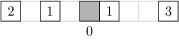
Figure 2: Example of avalanche process for a one-dimensional sandpile model (left, $\theta=7$), which is not pseudo-linear: the avalanche process may topple cells arbitrarily far on the right before going backwards to topple cells on the left end (right, instance of $\mathsf{1^{\text{st}}col\text{-}S\text{-}PRED}$ where arrows depict the avalanche process).

In dimension one, for any $c,c^{\prime}\in\mathbb{N}^{\mathbb{Z}}$, let ${\mathsf{odo}}(c,c^{\prime})|_{[x,y]}$ denote the restriction of ${\mathsf{odo}}(c,c^{\prime})$ to the interval $[x,y]$, with $x<y$ two cells in $\mathbb{Z}$.

Lemma 4.

For any one-dimensional sandpile model $\left\langle\mathcal{D},\mathcal{N},\theta\right\rangle$ and any configurations $c,c^{\prime}$ such that $c$ is within the elementary hypercube, $c\stackrel{{\scriptstyle*}}{{\to}}c^{\prime}$ and $c^{\prime}$ is stable, with $r=\max\{|v|_{\infty}\mid v\in\mathcal{N}\}$, knowing

• ${\mathsf{odo}}(c,c^{\prime})|_{[x-r,x-1]}$ and ${\mathsf{odo}}(c,c^{\prime})|_{[y+1,y+r]}$

for cells $x,y\in\mathbb{Z}$ such that $x+r\leq y$, allows to compute

• ${\mathsf{odo}}(c,c^{\prime})|_{[x,x+2r-1]}$ and ${\mathsf{odo}}(c,c^{\prime})|_{[y-2r+1,y]}$

in time $\mathcal{O}(y-x)$ on one processor.

Figure 3 provides a graphical illustration of the statement of Lemma 4.

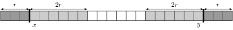
Figure 3: When every cell topples at most once, knowing which cells among $[x-r,x-1]$ and $[y+1,y+r]$ topple allows to compute which cells among $[x,x+2r-1]$ and $[y-2r+1,y]$ topple, where $r=\max{\left\{|v|_{\infty}\mid v\in\mathcal{N}\right\}}$ (Lemma 4).

Proof.

If one knows all topplings that may influence the topplings within $[x,y]$ (given by the assumptions ${\mathsf{odo}}(c,c^{\prime})|_{[x-r,x-1]}$ and ${\mathsf{odo}}(c,c^{\prime})|_{[y+1,y+r]}$, where $r$ is the radius of the sandpile model), it is possible to compute all topplings occurring within $[x,y]$. Furthermore, from Proposition 4, any cell topples at most once and hence the number of topplings is upper bounded by $y-x$, which in its turn is an upper bound on the number of computation steps. The condition $x+r<y$ ensures that the output is made of ${\mathsf{odo}}(c,c^{\prime})$ values within the interval $[x-r,y+r]$. ∎

Theorem 4.

For any one-dimensional sandpile model, $\mathsf{1^{\text{st}}col\text{-}S\text{-}PRED}\in{\mathsf{NC}}^{1}$.

Sketch.

Let us describe how to derive an ${\mathsf{NC}}^{1}$ algorithm for $\mathsf{1^{\text{st}}col\text{-}S\text{-}PRED}$ from Lemma 4. Let $c,x$ be the instance, and $c^{\prime}$ be the stable configuration such that $c\stackrel{{\scriptstyle*}}{{\to}}c^{\prime}$. For simplicity sake, assume that $c$ is $c+{\bf 1}_{{\left\{0\right\}}}$, and let $r=\max{\left\{|v|_{\infty}\mid v\in\mathcal{N}\right\}}$.

1. Compute, in parallel for every $y\in\mathbb{N}$ multiple of $r$, the function taking as input ${\mathsf{odo}}(c,c^{\prime})|_{[y-r,y-1]}$ and ${\mathsf{odo}}(c,c^{\prime})|_{[y+4r,y+5r-1]}$, and outputting ${\mathsf{odo}}(c,c^{\prime})|_{[y,y+2r-1]}$ and ${\mathsf{odo}}(c,c^{\prime})|_{[y+2r,y+4r-1]}$ (see picture below for a partial example with some $y$ multiple of $r$ and $z=y+4r$, on two copies of the configuration for clarity). From Lemma 4, each computation needs a constant time on one processor, and there are linearly many.
   

1. Compose them according to some binary tree: each function is of constant size (from Proposition 4, input is $2r$ bits and output is $4r$ bits), and we compose functions having some carefully chosen overlap. Let us denote $i_{1},i_{2},i_{3},i_{4},i_{5},i_{6},i_{7},i_{8},i_{9},i_{10}$ the respective portions of ${\mathsf{odo}}(c,c^{\prime})$ of size $r$ under consideration (see picture above), then the two functions are respectively: $i_{1},i_{6}\mapsto i_{2},i_{3},i_{4},i_{5}$ and $i_{5},i_{10}\mapsto i_{6},i_{7},i_{8},i_{9}$. With these two we can compute $i_{1},i_{5},i_{6},i_{10}\mapsto i_{2},i_{3},i_{4},i_{5},i_{6},i_{7},i_{8},i_{9}$, and fortunately the fixed point regarding $i_{5},i_{6}$ is uniquely determined by $i_{4},i_{7}$, according to a constant time application of Lemma 4 (remark that there may be an arbitrarily large gap between $i_{3}$ and $i_{4}$, and also between $i_{7}$ and $i_{8}$). Each composition deals with a constant number of functions of constant size, hence it takes a constant time. As there is a logarithmic number of levels in the composition, the overall process takes a logarithmic parallel time.

Now remark that no cell within $[-r,-1]$ nor $[n+1,n+r]$ topple, with $n$ the size of configuration $c$, hence ${\mathsf{odo}}(c,c^{\prime})|_{[-r,-1]}$ and ${\mathsf{odo}}(c,c^{\prime})|_{[n+1,n+r]}$ are fixed. In order to get the answer of whether cell $x=kr+k^{\prime}$ topples (for some unique $k,k^{\prime}\in\mathbb{N}$ with $0\leq k^{\prime}<r$), we consider two binary trees of compositions: one such that the root gives the function with input $[-r,-1],[kr,(k+1)r-1]$, and the other such that the root gives the function with input $[(k-1)r,kr-1],[n+1,n+r]$. The fixed point of their conjunction, resolved with the function with input $[(k-2)r,(k-1)r-1],[(k+1)r,(k+2)r-1]$ (again a constant time application of Lemma 4), tells whether ${\mathsf{odo}}(c,c^{\prime})(x)$ equals $0$ or $1$ (see picture below).

∎

As mentioned above, the generalization of the Theorem 4 to other prediction problems requires non-trivial extensions, because of multiple topplings at a cell which somehow should be handled in constant time computation. The proof of ${\mathsf{TC}}^{0}$-hardness from [52] also makes heavy use of multiple topplings, and as a consequence it does not generalize for free to an arbitrary one-dimensional sandpile model. We nevertheless conjecture that it also does.

Conjecture 3.

For any one-dimensional sandpile model, $\mathsf{PRED}$ is ${\mathsf{TC}}^{0}$-hard for ${\mathsf{AC}}^{0}$ reductions, and therefore not in ${\mathsf{AC}}^{1-\epsilon}$ for any constant $\epsilon>0$.

5 ${\mathsf{P}}$-completeness in dimension three and above

During his PhD thesis in the 1970s, Banks started to implement circuit computation using discrete dynamical systems working on grids (namely cellular automata) [4]. The intuition behind such implementations is quite straightforward: a sequence of cells change state in a chain of reactions to transport information; two flows of information can interact to create logic gates.

For simplicity, circuits are restricted to have the following characteristics:

• gates have fan in and fan out $2$,

• layered (information flows from one end to the other, layer by layer from inputs to output, without going backward),

• arranged on a grid layout.

Even with the previous constraints the prediction problems (SAM2CVP in [40]) are still ${\mathsf{P}}$-complete. Moore and Nilsson ported Banks’ technique to sandpile models in 1999 [54]. They used an adaptation to the grid of the computation encoding idea developed by Bitar, Goles and Margenstern in [5, 34].

Theorem 5 ([54]).

For von Neumann neighborhood $\mathcal{N}_{\text{VN}}$ of radius one and dimension $d\geq 3$, the problem $\mathsf{1^{\text{st}}col\text{-}S\text{-}PRED}$ is ${\mathsf{P}}$-complete.

Sketch.

The reduction is from $\mathsf{MCVP}$ (see Section 2.4), in the case of fan in and fan out 2, layered, on a grid. We will present the proof for dimension 3 in details, and explain at the end how it generalizes.

There are different types of gadgets to implement within sandpiles: wires, turns, and gates, or gates, plus diodes (to prevent unintended backward propagation of information) and multipliers (to get fan out 2). All these elements are presented as macrocells in Figure 4 (two top rows), and are embedded in a two-dimensional plane of the three-dimensional configuration. The non-planarity of the circuit requires (recall that $\mathsf{MPCVP}$ is in ${\mathsf{NC}}$, hence it is important that the circuit may not be planar) that wires cross each other, which is achieved using the third dimension (Figure 4 bottom row).

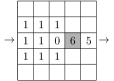
wire (0 or idle) wire (transmits 1) turn

and gate or gate diode multiplier

cross-over cross-over cross-over ($-1$ in $3^{\text{rd}}$ dimension) ($0$ in $3^{\text{rd}}$ dimension) ($1$ in $3^{\text{rd}}$ dimension)

Figure 4: Implementation of wires and gates with von Neumann neighborhood of radius one, in three dimensions ($\theta=6$). Only the cross-over gate uses the third dimension (it should be thought as three stacked layers), all other gates can be considered to live at coordinate $0$ in the third dimension. A wire is implemented as a simple chain of reactions of cell topplings: when it is triggered it transmits a 1, if not (i.e. it remains stable) it transmits a 0. Arrows indicate fan in and fan out (input and output pairs are identified in the cross-over gate: a signal coming from input $a$ (resp. $b$) results in a signal going to output $a$ (resp. $b$), independently of each other), empty cells contain no sand grain. Remark that appart from central cells of cross-overs, initialy empty cells will not topple.

Now the idea is that by replacing circuit elements with macrocells we can have a single grain addition triggering a wire that can be multiplied to implement the input constants on the first layer, which can be connected to gate on the second layer, etc, until the output gate which is simply a wire with the questionned cell in the center. As noted in [53], diodes should be added between layers to prevent backward propagation of information (specificaly to prevent false 1).

To finish the reduction, we would like to insist on the fact that crossing of wires in the third dimension is only necessary to overcome the non-planarity of $\mathsf{MCVP}$. In fact, it is equivalent to have a crossing or a negation gate:

• In [40] on $\mathsf{PCVP}$: “A planar xor circuit can be built from two each of and, or, and not gates; a planar cross-over circuit can be built from three planar xor circuits”.

• In [54] Moore and Nilsson wrote: “Using a double-wire logic where each variable corresponds to a pair of wires carrying $x$ and $\bar{x}$, [Bitar, Goles and Margenstern] implement negation as well by crossing the two wires”.

We prefer to imagine a single-wire logic, with cross-over of wires in the third dimension. Cell topplings correspond to the circuit computation (truth value 1 transmitted from layer to layer, going through gates), and the circuit outputs 1 if and only if the questioned cell topples.

This reduction is performed in constant parallel time (in ${\mathsf{AC}}^{0}$): each constant size part of the circuit is converted to a sandpile sub-configuration (macrocell) of constant size placed at a fixed position, hence in a PRAM model each processor can handle one such part (there are polynomially many) in constant time.

In order to generalize the proof to any dimension $d\geq 3$, simply remark that the same construction can be embedded in only three dimensions among many, with coordinate zero in all other dimensions, provided one adapts the sand content of non-empty cells according to $\theta$ (plus two grains for any dimension above three). ∎

From the proof above we can notice that to simulate a circuit (instance of $\mathsf{MCVP}$), von Neumann sandpile model of radius one and dimension $d\geq 3$ undergoes a somewhat simple dynamics:

• only three dimensions are used (mainly two),

• only cell contents $0$, $\theta-2$ and $\theta-1$ appear in macrocells,

• the strong monotonicity of Proposition 4 holds (any cell topples at most once),

• we have wires and gates organized in successive layers from inputs to output,

• all directions of information are known in the reduction,

• there are diodes everywhere so that information flows in exactly one direction.

As a consequence we can consider that the evolution of the obtained $\mathsf{1^{\text{st}}col\text{-}S\text{-}PRED}$ instance $(c,x)$ verifies very restrictive conditions. Let us consider that there is a diode between every pair of gates presented on Figure 4. Then the flow of information between gates and layers is totally fixed, and we can almost claim that for any pair of neighbouring cells it is known which one would topple first (in the case both topple). However this is not completely accurate, as in or gates for example: if only one of the two inputs transmits a 1 signal, then some cells going to the other input topple “backward”. This is clearly not an issue nor an important feature. We formalize how another sandpile model with $d\geq 3$ can perform the same kind of circuit simulation as von Neumann of radius one in three dimensions.

Lemma 5.

If a sandpile model of neighborhood $\mathcal{N}$ has three linearly independent $x,y,z\in\mathcal{N}$ such that $ax+by+cz\notin\mathcal{N}$ for any $a,b,c\in\mathbb{Z}$, except when:

$$a=\pm 1,b=0,c=0\quad\text{or}\quad a=0,b=\pm 1,c=0\quad\text{or}\quad a=0,b=0,c=\pm 1,$$

then it has a ${\mathsf{P}}$-complete $\mathsf{1^{\text{st}}col\text{-}S\text{-}PRED}$ problem.

Proof.

Let us add two modifications to the circuit simulation of von Neumann radius one in three dimensions presented in the proof of Theorem 5, so that it fits the present context. First, up to a straightforward layout shift, we can embed all planar gates from Figure 4 with only two directions of information transmission: $x$ and $y$. Second, the third direction $z$ is used for the cross-over, which shifts in this direction the rest of the sandpile implementation of the circuit (see Figure 5). We can simply assume that there is one cross-over per layer to fix the $z$-shift everywhere. These coordinate changes do not change the computational complexity of the problem.

Figure 5: von Neumann radius one in three dimensions simulating a layered circuit, with information flowing in three directions which will correspond to $x,y,z$. Light colored cubes contain $5$ grains ($\theta-1$), darker cubes contain $4$ grains ($\theta-2$), and black cubes are $\{0\}^{d}$ and the questioned cell (they both contain $5=\theta-1$ grains). The circuit is implemented with macrocells of size $5\times 5$, and a $z$-shift of $2$ units. Arrows indicate the direction of information flow.

A sandpile model with such $x,y,z$ can simulate at a local level von Neumann of radius one in three dimensions (neighbours are given by $x,y,z$), itself simulating a circuit as in Figure 5. Indeed, information flows in at most one direction ($x,y,z\in\mathcal{N}$ implies that information flows in the expected direction, and the reverse direction may or may not be in $\mathcal{N}$, as it is nor important nor an issue), and in other cases transmissions do not interfere one with another from the condition that $ax+by+cz\notin\mathcal{N}$.

Hence taking cells from the three-dimensional grid generated by $\{x,y,z\}$, and placing:

• $\theta-\mathcal{D}(u)$ grain with $u\in\{x,y,z\}$ for cells with $5$ grains in von Neumann ($\theta-1$ in that model), depending on the expected in-neighbor $u$, or two in-neighbors and the minimum number of sand grains received from one of them,

• $\theta-\mathcal{D}(u)-\mathcal{D}(v)$ grains with $u,v\in\{x,y,z\}$ for cells with $4$ grains in von Neumann ($\theta-2$ in that model), depending on the two expected in-neighbors $u,v$,

• no grain for empy cells in von Neumann,

the sandpile model can simulate von Neumann radius one in three dimensions, itself simulating a circuit. The transformation is performed in constant parallel time, ${\mathsf{AC}}^{0}$. ∎

It follows that all $d$-dimensional sandpile models with $d\geq 3$ (verifying Equation (1)) are ${\mathsf{P}}$-complete to predict.

Corollary 2.

$\mathsf{1^{\text{st}}col\text{-}S\text{-}PRED}$, $\mathsf{S\text{-}PRED}$ and $\mathsf{PRED}$ are ${\mathsf{P}}$-complete for any sandpile model in dimension $d\geq 3$.

Proof.

Let $M=\left\langle\mathcal{N},\mathcal{D},\theta\right\rangle$ be a sandpile model in dimension $d\geq 3$, and let $\lVert u\rVert$ denote the Euclidean norm ($\ell_{2}$-norm) of cell $u\in\mathbb{Z}^{d}$. We define $x,y,z$ as follows.

• $x$ is a cell inside $\mathcal{N}$ of maximal norm, i.e.

  $$x\in\arg\max_{u\in\mathcal{N}}\{\lVert u\rVert\}.$$

• $y$ is a cell inside $\mathcal{N}$ of maximal norm when projected onto the $(d-1)$-dimensional subspace orthogonal to the line defined by points $\{0\}^{d},x$, i.e.

  $$y\in\arg\max_{u\in\mathcal{N}}\{\lVert p_{x^{\bot}}(u)\rVert\}$$

  with $p_{x^{\bot}}$ the projection onto $\{v\in\mathbb{Z}^{d}\mid v\cdot x=0\}$.

• $z$ is a cell inside $\mathcal{N}$ of maximal norm when projected onto the $(d-2)$-dimensional subspace orthogonal to the plane defined by points $\{0\}^{d},x,y$, i.e.

  $$z\in\arg\max_{u\in\mathcal{N}}\{\lVert p_{xy^{\bot}}(u)\rVert\}$$

  with $p_{xy^{\bot}}$ the projection onto $\{v\in\mathbb{Z}^{d}\mid\forall a,b\in\mathbb{Z}:v\cdot(ax+by)=0\}$.

From Equation (1) such $x,y,z$ exist and are non-colinear.

Furthermore, it is always possible to choose $x,y,z$ such that $ax+by+xz\notin\mathcal{N}$ for $a,b,c\in\mathbb{Z}$ different than in the statement of Lemma 5. Indeed, a linear combination with two non-null components such that $ax+by+xz\in\mathcal{N}$ either gives another vector of maximal norm that may replace one of $y,z$ (if the projection onto $x^{\bot}$ or $xy^{\bot}$ is negative on all components, then it becomes positive on one component), or contradicts the maximality of $x$, $y$ or $z$ (if the projection onto $x^{\bot}$ or $xy^{\bot}$ is positive on one component).

From Lemma 5 we can conclude that $\mathsf{1^{\text{st}}col\text{-}S\text{-}PRED}$ is ${\mathsf{P}}$-complete, and Proposition 6 implies that $\mathsf{S\text{-}PRED}$ and $\mathsf{PRED}$ are also ${\mathsf{P}}$-complete. ∎

Writting formal proofs of ${\mathsf{P}}$-completeness via reduction from some $\mathsf{CVP}$ problem requires a substantial amount of precisions, and some obvious details are often not mentionned, though they may be key in other contexts (such as the symmetry of von Neumann neighborhood and the dynamics of layers equipped with diodes in the proof of Theorem 5). In [38] the authors present a general framework to prove ${\mathsf{P}}$-completeness using Banks’ technic in cellular automata. A neat formalism is introduced, defining what is meant by “simulating a gate set”. Then results are presented, of the form: if a cellular automaton can simulate a set of gates $A$ (for example $A={\left\{\text{{\em and}, {\em or}, {\em cross-over}}\right\}}$), then its prediction problem is hard for some class $C$ (in this example $C={\mathsf{P}}$). A novel distinction appears to be fundamental for the dynamical complexity of discrete dynamical systems: whether is is possible to build re-usable simulation of wires and gates, or not (weak simulation). Indeed, re-usable simulation brings ${\mathsf{P}}$-completeness from and and or gates only, because it is possible to build a planar cross-over gadget with re-usable simulation of monotones gates. This result is surprising compared to the characterization of Boolean gates allowing planar cross-over presented in [51], which is not the case of any set of monotone gates. It comes from the dynamical nature of circuit simulation with discrete dynamical systems, and the possibility to re-use wires that is not present in the original circuit model.

In the context of sandpile models, circuit simulation in two dimensions is harder to achieve precisely because of the difficulty to create cross-over (see Section 6). The planar cross-over gadget in re-usable simulation seems however difficult to apply to sandpile models, since it exploits delays in signal transmissions, which is in contradiction with the Abelian Proposition 2 telling that order of topplings do not matter.

6 The two-dimensional case

No two-dimensional sandpile model is known to be efficiently predictable in parallel, i.e. such that its prediction problem is in ${\mathsf{NC}}$. As we will see, some slight extensions of von Neumann sandpile model of radius one turn out to have ${\mathsf{P}}$-complete prediction problems, but the computational complexity of predicting the original model of Bak, Tang and Wiesenfeld [2] remains open. This is considered as the major open problem regarding the complexity of prediction in sandpile models. It is also open for Moore neighborhood of radius one.

Open question 4.

Consider the von Neumann and Moore sandpile models in dimension two. Are $\mathsf{PRED},\mathsf{S\text{-}PRED}$ and $\mathsf{1^{\text{st}}col\text{-}S\text{-}PRED}$ in ${\mathsf{NC}}$, ${\mathsf{P}}$-complete, or neither?

The third possibility comes from the fact that under the assumption ${\mathsf{NC}}\neq{\mathsf{P}}$, there exist problems in ${\mathsf{P}}$ that are neither in ${\mathsf{NC}}$ nor ${\mathsf{P}}$-complete [59]. The difficulty in applying Banks’ approach here is to overcome planarity imposed by the two-dimensional grid with von Neumann or Moore neighborhood, since the monotone planar circuit value problem ($\mathsf{MPCVP}$) is in ${\mathsf{NC}}$. In fact, it has been proven to be impossible to perform elementary forms of signal cross-over in this model [32]. The precise statement is a bit technical to state, but corresponds neatly to the intuition of having two potential sequences of cell topplings representing two wires that may convey a bit of information, and cross each other without interacting (i.e. they independently transport information). We shall call these elementary forms of signaling since other ways to encode the transportation of information in sandpile may be found, but as emphasized by Delorme and Mazoyer in [15] to quantify over such possible encodings and give fully general impossibility results, is an issue.

Theorem 6 ([32]).

It is impossible to perform elementary forms of signal cross-over in von Neumann and Moore neighborhoods of radius one.

However, as soon as the neighborhood is a bit extended, it turns out to be possible to perform a cross-over, as expressed in the following result.

Theorem 7 ([26, 32]).

In two dimensions, von Neumann neighborhood of radius $r\geq 2$ has ${\mathsf{P}}$-complete prediction problems $\mathsf{1^{\text{st}}col\text{-}S\text{-}PRED}$, $\mathsf{S\text{-}PRED}$ and $\mathsf{PRED}$. It is also the case for the non-deterministic Kadanoff sandpile model of radius $r\geq 2$.

In dimension two, the radius $r$ Kadanoff sandpile model is defined in [26] as the non-deterministic application of the one-dimensional Kadanoff sandpile model (see Remark 3) in the two directions of the plane, plus a monotonicity property that needs to be preserved, and the prediction problem asks for the existence of an avalanche reaching the questioned cell (in the circuit implementation any cell topples at most once, hence it corresponds to $\mathsf{1^{\text{st}}col\text{-}S\text{-}PRED}$).

Augmenting a little bit the neighborhood allows to perform cross-over and simulate $\mathsf{MCVP}$ instances. More has been said in [57] on cross-over impossibility, and as an immediate corollary we have that elementary forms of signal cross-over are impossible when the graph supporting the dynamics is planar (which is the case for von Neumann of radius one, but not of greater radii).

Lemma 6 ([57]).

If a sandpile model can implement an elementary form of cross-over, then it can implement one such that the two elementary signals do not have any cell in common. This is true on any Eulerian digraph.

Also, the fact that a neighborhood can or cannot perform cross-over (given the distribution $\mathcal{D}_{1}$ sending $1$ grain to each out-neighbor) is intrinsically discrete. Indeed, if one thinks about the shape of some neighborhood as a continuous two-dimensional region that we can scale and place on a grid to get a (discrete) neighborhood, then impossibility to perform cross-over cannot be characterized in terms of shape.

Theorem 8 ([57]).

Any shape can perform cross-over starting from some scaling ratio.

Even a circle, with a big enough scaling ratio, gives a neighborhood that can perform cross-over and have a ${\mathsf{P}}$-complete prediction problem.

The precise conditions for ${\mathsf{P}}$-completeness of the prediction problems in two-dimensions are still to be found. Having a precise characterization would be of great interest to shed light on the universality of Banks’ approach: if a sandpile model has a ${\mathsf{P}}$-complete prediction problem, then for sure it can simulate circuits. But are there ways of doing so with non-elementary forms of signaling?

In [54], after recalling that $\mathsf{MPCVP}$ (monotone planar $\mathsf{CVP}$) is in ${\mathsf{NC}}$, Moore and Nilsson gave insights on the possibilities to reduce circuit simulation to sandpile dynamics for von Neumann radius one in two dimensions: “two-dimensional sandpiles differ from planar Boolean circuits in two ways. First, connections between sites are bidirectional. Secondly, a given site can change a polynomial number of times in the course of the sandpile’s evolution. Thus we really have a three-dimensional Boolean circuit of polynomial depth, with layers corresponding to successive steps in the sandpile’s space-time.”

Let us conclude this section with a lower bound on the complexity of two-dimensional sandpile models. As noticed by Miltersen in [52], a corollary of Theorem 5 is that the two-dimensional von Neumann sandpile model of radius one is ${\mathsf{NC}}^{1}$-hard since it can simulate monotone planar circuits (an $\mathsf{MPCVP}$ instance can be reduced to a $\mathsf{1^{\text{st}}col\text{-}S\text{-}PRED}$ instance with an ${\mathsf{AC}}^{0}$ algorithm, without implementing cross-over), and $\mathsf{MPCVP}$ is ${\mathsf{NC}}^{1}$-hard since evaluating a Boolean formula (for which the circuit is a tree) is ${\mathsf{NC}}^{1}$-complete [8]. From Lemma 5 and Corollary 2 this observation extends to any two-dimensional sandpile model, since the third dimension is used exclusively for cross-over gates.

Theorem 9.

For any two-dimensional sandpile model, $\mathsf{1^{\text{st}}col\text{-}S\text{-}PRED}$, $\mathsf{S\text{-}PRED}$ and $\mathsf{PRED}$ are ${\mathsf{NC}}^{1}$-hard.

7 Simulations between sandpile models

As seen in the previous sections the prediction problems for sandpile models are dimension sensitive but once the dimension is fixed they turn out to be closely related to one another. This section provides a notion of simulation between sandpile models and show that simulating a run of a sandpile model by another with different parameters (neighborhood or distribution) has a polynomial cost. Only sequential update policy is considered in this section. Moreover, all finite configurations mentioned are intended to belong to the elementary hypercube. For this reason those hypothesis is omitted from the statements.

Given a configuration $c\in\mathbb{N}^{\mathbb{Z}^{d}}$, a firing sequence for $c$ is a sequence $(x_{1},x_{2},\ldots,x_{n})\in\mathbb{Z}^{d}$ of cells such that there exist configurations $c_{1}=c,c_{2},\ldots,c_{n}$ such that $c_{i}\stackrel{{\scriptstyle x_{i}}}{{\rightharpoonup}}c_{i+1}$ for all $i\in{\left\{1,\ldots,n-1\right\}}$ and

1. $c_{1}(x_{1})=\theta-1$;

2. $x_{i+1}-x_{i}\in\mathcal{N}$ for all $i\in{\left\{1,2,\ldots,n-1\right\}}$;

3. $c_{i}(x_{i})=\theta$ for $i\in{\left\{2,\ldots,n\right\}}$.

Remark that when a firing sequence has been triggered i.e. when a sand grain has been added at $x_{1}$ in $c_{1}$, grains may be distributed on set of cells which are in the neighborhood of some element of the sequence. The hitting set collects precisely this information. More formally, the hitting set induced by a firing sequence $(x_{1},x_{2},\ldots,x_{n})\in\mathbb{Z}^{d}$ for a finite configuration $c$ is the set of pairs $(x,u)$ where $x\in\mathbb{Z}^{d}$ is a cell and $u\in\mathbb{N}\setminus{\left\{0\right\}}$ is the total number of grains that $x$ has received when all the cells of the firing sequence have been fired. An $\mathcal{N}$-path from the cell $x\in\mathbb{Z}^{d}$ to $y\in\mathbb{Z}^{d}$ is an sequence $(z_{1},z_{2},\ldots,z_{n})$ of cells such that $z_{1}=x$, $z_{n}=y$ and $z_{i+1}-z_{i}\in\mathcal{N}$ for all $i\in{\left\{1,\ldots,n-1\right\}}$. Remark that if $\mathcal{N}$ is complete, then there always exists an $\mathcal{N}$-path between any pair of cells. Given a finite configuration $c$, let $V(c)\subset\mathbb{Z}^{d}$ be the convex hull of points $x\in\mathbb{Z}^{d}$ such that $c_{x}\neq 0$. A detector cell $y$ for a finite configuration $c$ with hitting set $H$ is a cell such that there exists an integer $u>0$ such that $(y,u)\in H$ and $y\notin V(c)$. In other words, a detector cell for a finite configuration $c$ is a cell which is “outside” $c$ and which may receive a sand grain if some cell $z$ “inside” $c$ is triggered. Of course, if given a finite configuration $c$, for all $x\in\mathbb{Z}^{d}$ we have that $c+{\bf 1}_{x}$ is stable, then $c$ has no detector cells. Figure 6 illustrates all these recent notions.

Figure 6: Sandpile model with $\theta=6$, neighborhood and distribution function as depicted on bottom left. The evolution starts from the finite configuration on top left (cells not drawn are supposed to contain $0$). Dark-grayed cells (taken in the order indicated by $\mapsto$) are the firing sequence. In the final stable configuration, cells in the hitting set have their content in bold face, while detector cells have a light-gray background.

Given two sandpile models $M_{1}\equiv\left\langle\mathcal{N}_{1},\mathcal{D}_{1},\theta_{1}\right\rangle$ and $M_{2}\equiv\left\langle\mathcal{N}_{2},\mathcal{D}_{2},\theta_{2}\right\rangle$, we say that $M_{2}$ simulates $M_{1}$ if there exist a computable transformation $h:\mathbb{N}^{\mathbb{Z}^{d}}\to\mathbb{N}^{\mathbb{Z}^{d}}$ such that for all finite configurations $c,c^{\prime}\in\mathbb{N}^{\mathbb{Z}^{d}}$ and all pair of cells $x,y\in\mathbb{Z}^{d}$ such that

1. $c,c^{\prime}$ are stable for $M_{1}$;

2. $c+{\bf 1}_{x}\stackrel{{\scriptstyle*}}{{\rightharpoonup}}c^{\prime}$ according to $M_{1}$;

3. $y$ is a detector cell for $c$;

and there exists a finite configuration $c^{\prime\prime}$ such that

1. $h(c),c^{\prime\prime}$ are stable for $M_{2}$;

2. $h(c)+{\bf 1}_{x}\stackrel{{\scriptstyle*}}{{\rightharpoonup}}c^{\prime\prime}$ according to $M_{2}$;

3. if $c^{\prime}(y)>0$ then $c^{\prime\prime}(y)>0$.

In other words, $M_{2}$ simulates $M_{1}$ if starting on a computable encoding of an initial configuration $c$ of $M_{1}$ the stable configuration which is reached afterwards contains the same bit of information in the detector cell $y$ as $M_{1}$.

Lemma 7.

Consider two complete neighborhoods $\mathcal{N}_{1},\mathcal{N}_{2}\subset\mathbb{Z}^{d}$ such that $\mathcal{N}_{1}=\mathcal{N}_{2}\cup{\left\{u\right\}}$ for $u\in\mathbb{Z}^{d}$. For any sandpile model $M_{2}\equiv\left\langle\mathcal{N}_{2},\mathcal{D}_{2},\theta_{2}\right\rangle$, there exists a sandpile model $M_{1}\equiv\left\langle\mathcal{N}_{1},\mathcal{D}_{1},\theta_{1}\right\rangle$ which simulates $M_{2}$.

Proof.

Let $c\in\mathbb{N}^{\mathbb{Z}^{d}}$ be a stable configuration for $M_{2}$ and choose $x\in\mathbb{Z}^{d}$. Let $c^{\prime}$ be such that $c+{\bf 1}_{x}\stackrel{{\scriptstyle*}}{{\rightharpoonup}}c^{\prime}$ according to $M_{2}$ and let $y$ be a detector cell for $c^{\prime}$. Let $F_{2}$ be the firing sequence $F_{2}\equiv(x_{1},\ldots,x_{n})$ associated with $c+{\bf 1}_{x}$ and let $H_{2}$ be the induced hitting set. The idea is to take the same firing sequence also for the model $M_{1}$ that we are going to define but to craft the configuration $c^{\prime}$ realizing the circuit for $M_{1}$ in such a way to prevent unnecessary supplementary firings or before-time firings because of grains dropped forward by the $u$ component of the neighborhood. Hence, let $F_{1}=F_{2}$ be the firing sequence for the model $M_{1}$. Define $\theta_{1}=\theta_{2}+1$ and

$$\forall v\in\mathcal{N}_{1},\;\mathcal{D}_{1}(v)=\begin{cases}\mathcal{D}_{2}(v)&\text{if }v\in\mathcal{N}_{2}\\ 1&\text{otherwise.}\end{cases}$$

Let us build a new finite configuration $c^{\prime\prime}$ as follows

$$\forall z\in\mathbb{Z}^{d},\;c^{\prime\prime}(z)=\begin{cases}\theta_{1}-1&\text{if }z=x\\ \theta_{1}-v&\text{if }z\in F_{1}\text{ and }(z,v)\in H_{2}\\ 0&\text{otherwise.}\end{cases}$$

Let $c^{\prime\prime\prime}$ be the stable configuration such that $c^{\prime\prime}\stackrel{{\scriptstyle*}}{{\rightharpoonup}}c^{\prime\prime\prime}$ according to $M_{1}$. It is clear that $c^{\prime}(y)>0$ implies $c^{\prime\prime\prime}(y)>0$. Indeed, if $c^{\prime}(y)>0$, then there exists $x_{i}\in F_{1}=F_{2}$ such that $y-x_{i}\in\mathcal{N}_{2}\subset\mathcal{N}_{1}$. Hence, $c^{\prime\prime\prime}(y)>0$. ∎

The proofs of the following lemmas are very similar to the ones of previous lemmas and thus they are omitted.

Lemma 8.

Consider a neighborhood $\mathcal{N}\subseteq\mathbb{Z}^{d}$ (not necessarily complete) and a sandpile model $M_{1}\equiv\left\langle\mathcal{N},\mathcal{D}_{1},\theta_{1}\right\rangle$. Define the model $M_{2}\equiv\left\langle\mathcal{N},\mathcal{D}_{2},\theta_{1}+k\right\rangle$ for some $k\in\mathbb{N}_{+}$ and such that

1. there exists a unique $u\in\mathcal{N}$ for which $\mathcal{D}_{2}(u)=\mathcal{D}_{1}(u)+k$;

2. $\forall v\in\mathcal{N},\;(u\neq v)\Rightarrow\mathcal{D}_{2}(v)=\mathcal{D}_{1}(v)$.

Then, $M_{2}$ simulates $M_{1}$.

Lemma 9.

Consider a neighborhood $\mathcal{N}\subseteq\mathbb{Z}^{d}$ (not necessarily complete) and a sandpile model $M_{1}\equiv\left\langle\mathcal{N},\mathcal{D}_{1},\theta_{1}\right\rangle$. Define the model $M_{2}\equiv\left\langle\mathcal{N},\mathcal{D}_{2},\theta_{2}\right\rangle$ such that

1. there exists a unique $u\in\mathcal{N}$ for which $\mathcal{D}_{2}(u)=\mathcal{D}_{1}(u)-k>0$ for some $k\in\mathbb{N}_{+}$;

2. $\forall v\in\mathcal{N},\;(u\neq v)\Rightarrow\mathcal{D}_{2}(v)=\mathcal{D}_{1}(v)$;

3. $\theta_{2}=\theta_{1}-k$.

Then, $M_{2}$ simulates $M_{1}$.

Remark that from a computational complexity point of view, the constructions of the previous lemma come at no cost. However, each single simulation has a cost which essentially consists in computing the firing sequence for the original system (the hitting set can be computed at a constant multiplicative cost while computing the firing sequence). By Theorem 1, this can be done in polynomial time (using a stack for example).

The notion of simulation between sandpile models induces a preorder structure on the set of sandpile models in the same dimension. It is an interesting research direction to explore the properties of such an order and see if and under which form there exists a notion of universality.

8 Undecidability on infinite configurations

A further generalisation of sandpile models consists in relaxing the finiteness of the initial configuration. As noted in [9], allowing any configuration initially written on the tape of the Turing machine would make the prediction problem trivially undecidable in any dimension, and restricting to periodic configurations comes down to studying a finite region on a torus and is therefore decidable in any dimension (since given a fixed number of sand grains there are finitely many configurations). On the other hand, when the initial configuration given as input to the prediction problem is ultimately periodic (i.e. periodic except on a finite region), then the following result holds.

Theorem 10 ([9]).

$\mathsf{PRED}$ extended to ultimately periodic configurations (the input consists in the finite non-periodic region, plus the finite periodic pattern repeated all around) in dimension three is undecidable.

Finally, if we further relax the number-conservation property and allows the distribution functions to “eat” grains, then one obtains sand automata [12]. Without going into the details of their precise definition (which is a bit involved), we can just recall that they are a special type of cellular automata particularly adapted to the sandpile “playground” [21, 20]. The following result is interesting in our context.

Theorem 11 ([13, 14]).

Ultimate (temporal) periodicity is undecidable for sand automata on finite configurations.

This last result tells that (somewhat unsurprisingly) sand automata are highly unpredictable.

References

- [1] L. Acerbi, A. Dennunzio, and E. Formenti. Shifting and lifting of cellular automata. In Proceedings of CiE’2007, volume 4497 of LNCS, pages 1–10, 2007.
- [2] P. Bak, C. Tang, and K. Wiesenfeld. Self-organized criticality: An explanation of the 1/f noise. Physical Review Letters, 59:381–384, 1987.
- [3] P. Bak, C. Tang, and K. Wiesenfeld. Self-organized criticality. Physical Review A, 38(1):364–374, 1988.
- [4] E. R. Banks. Information processing and transmission in cellular automata. PhD thesis, Massachusetts Institute of Technology, 1971.
- [5] J. Bitar and E. Goles. Parallel chip firing games on graphs. Theoretical Computer Science, 92(2):291 – 300, 1992.
- [6] A. Björner, L. Lovász, and P. W. Shor. Chip-firing games on graphs. European Journal of Combinatorics, 12(4):283–291, 1991.
- [7] A. Björner and L. Lovász. Chip-firing games on directed graphs. Journal of Algebraic Combinatorics, 1:305–328, 1992.
- [8] S. R. Buss. The boolean formula value problem is in alogtime. In Proceedings of STOC ’1987, pages 123–131, 1987.
- [9] H. Cairns. Some halting problems for abelian sandpiles are undecidable in dimension three. SIAM Journal on Discrete Mathematics, 32(4):2636–2666, 2018.
- [10] G. Cattaneo, G. Chiaselotti, A. Dennunzio, E. Formenti, and L. Manzoni. Non uniform cellular automata description of signed partition versions of ice and sand pile models. In Proceedings of ACRI’2014, volume 8751 of LNCS, pages 115–124, 2014.
- [11] G. Cattaneo, A. Dennunzio, E. Formenti, and J. Provillard. Non-uniform cellular automata. In Proceedings of LATA’2009, volume 5457 of LNCS, pages 302–313, 2009.
- [12] J. Cervelle and E. Formenti. On sand automata. In Proceedings of STACS’2003, volume 2607 of LNCS, pages 642–653, 2003.
- [13] J. Cervelle, E. Formenti, and B. Masson. Basic properties for sand automata. In Proceedings of MFCS’2005, volume 3618 of LNCS, pages 192–211. Springer, 2005.
- [14] J. Cervelle, E. Formenti, and B. Masson. From sandpiles to sand automata. Theoretical Computer Science, 381(1-3):1–28, 2007.
- [15] M. Delorme and J. Mazoyer. Signals on cellular automata. In Andrew Adamatzky, editor, Collision-based Computing, pages 231–275. Springer-Verlag, 2002.
- [16] A. Dennunzio. From one-dimensional to two-dimensional cellular automata. Fundam. Inform., 115(1):87–105, 2012.
- [17] A. Dennunzio, P. Di Lena, E. Formenti, and L. Margara. Periodic orbits and dynamical complexity in cellular automata. Fundam. Inform., 126(2-3):183–199, 2013.
- [18] A. Dennunzio, E. Formenti, E. Manzoni, G. Mauri, and A. E. Porreca. Computational complexity of finite asynchronous cellular automata. Theoretical Computer Science, 664:131–143, 2017.
- [19] A. Dennunzio, E. Formenti, and J. Provillard. Local rule distributions, language complexity and non-uniform cellular automata. Theoretical Computer Science, 504:38–51, 2013.
- [20] A. Dennunzio, P. Guillon, and B. Masson. Stable dynamics of sand automata. In Proceedings of TCS’2008, volume 273 of IFIP, pages 157–169, 2008.
- [21] A. Dennunzio, P. Guillon, and B. Masson. Sand automata as cellular automata. Theoretical Computer Science, 410(38-40):3962–3974, 2009.
- [22] D. Dhar. Self-organized critical state of sandpile automaton models. Physical Review Letters, 64:1613–1616, 1990.
- [23] D. Dhar. The abelian sandpile and related models. Physica A: Statistical Mechanics and its Applications, 263(1-4):4–25, 1999.
- [24] D. Dhar, P. Ruelle, S. Sen, and D.-N. Verma. Algebraic aspects of abelian sandpile models. Journal of Physics A: Mathematical and General, 28(4):805, 1995.
- [25] P. W. Dymond and S. A. Cook. Complexity theory of parallel time and hardware. Information and Computation, 80(3):205 – 226, 1989.
- [26] E. Formenti, E. Goles, and B. Martin. Computational complexity of avalanches in the Kadanoff sandpile model. Fundamenta Informaticae, 115(1):107–124, 2012.
- [27] E. Formenti, B. Masson, and T. Pisokas. Advances in symmetric sandpiles. Fundamenta Informaticae, 76(1-2):91–112, 2007.
- [28] E. Formenti, K. Perrot, and E. Rémila. Computational complexity of the avalanche problem on one dimensional Kadanoff sandpiles. In Proceedings of AUTOMATA’2014, volume 8996 of LNCS, pages 21–30, 2014.
- [29] E. Formenti, K. Perrot, and E. Rémila. Computational complexity of the avalanche problem for one dimensional decreasing sandpiles. Journal of Cellular Automata, 13:215–228, 2018.
- [30] Enrico Formenti, Benoît Masson, and Theophilos Pisokas. On symmetric sandpiles. In Proceedings of ACRI’2006, volume 4173 of LNCS, pages 676–685. Springer, 2006.
- [31] M. Furst, J. B. Saxe, and M. Sipser. Parity, circuits, and the polynomial-time hierarchy. Mathematical systems theory, 17(1):13–27, 1984.
- [32] A. Gajardo and E. Goles. Crossing information in two-dimensional sandpiles. Theoretical Computer Science, 369(1-3):463–469, 2006.
- [33] E. Goles, D. Maldonado, P. Montealegre, and N. Ollinger. On the computational complexity of the freezing non-strict majority automata. In Proceedings of AUTOMATA’2017, pages 109–119, 2017.
- [34] E. Goles and M. Margenstern. Sand pile as a universal computer. International Journal of Modern Physics C, 7(2):113–122, 1996.
- [35] E. Goles and M. Margenstern. Universality of the chip-firing game. Theoretical Computer Science, 172(1-2):121–134, 1997.
- [36] E. Goles and P. Montealegre. Computational complexity of threshold automata networks under different updating schemes. Theoretical Computer Science, 559:3–19, 2014.
- [37] E. Goles and P. Montealegre. A fast parallel algorithm for the robust prediction of the two-dimensional strict majority automaton. In Proceedings of ACRI’2016, pages 166–175, 2016.
- [38] E. Goles, P. Montealegre, K. Perrot, and G. Theyssier. On the complexity of two-dimensional signed majority cellular automata. Journal of Computer and System Sciences, 91:1–32, 2017.
- [39] E. Goles, P. Montealegre-Barba, and I. Todinca. The complexity of the bootstraping percolation and other problems. Theoretical Computer Science, 504:73–82, 2013.
- [40] R. Greenlaw, H. J. Hoover, and W. L. Ruzzo. Limits to Parallel Computation: P-Completeness Theory. Oxford University Press, Inc., 1995.
- [41] D. Griffeath and C. Moore. Life without death is p-complete. Complex Systems, 10, 1996.
- [42] J. Håstad. Computational Limitations of Small-depth Circuits. MIT Press, 1987.
- [43] J. Jájá. An introduction to parallel algorithms. Addison-Wesley, 1992.
- [44] C. G. Langton. Computation at the edge of chaos: Phase transitions and emergent computation. Physica D: Nonlinear Phenomena, 42(1):12 – 37, 1990.
- [45] L. Levine, W. Pegden, and C. K. Smart. Apollonian structure in the abelian sandpile. Geometric and Functional Analysis, 26(1):306–336, 2016.
- [46] L. Levine, W. Pegden, and C. K. Smart. The apollonian structure of integer superharmonic matrices. Annals of Mathematics, 186(1):1–67, 2017.
- [47] L. Levine and Y. Peres. Laplacian growth, sandpiles, and scaling limits. Bulletin of the American Mathematical Society, 54(3):355–382, 2017.
- [48] J. Machta and R. Greenlaw. The computational complexity of generating random fractals. Journal of Statistical Physics, 82(5):1299–1326, 1996.
- [49] J. Machta and K. Moriarty. The computational complexity of the lorentz lattice gas. Journal of Statistical Physics, 87(5):1245–1252, 1997.
- [50] J. Matcha. The computational complexity of pattern formation. Journal of Statistical Physics, 70(3):949–966, 1993.
- [51] W. F. McColl. Planar crossovers. IEEE Transactions on Computers, C-30(3):223–225, 1981.
- [52] P. B. Miltersen. The computational complexity of one-dimensional sandpiles. In Proceedings of CiE’2005, pages 342–348, 2005.
- [53] C. Moore. Majority-vote cellular automata, ising dynamics, and p-completeness. Journal of Statistical Physics, 88(3):795–805, 1997.
- [54] C. Moore and M. Nilsson. The computational complexity of sandpiles. Journal of Statistical Physics, 96:205–224, 1999. 10.1023/A:1004524500416.
- [55] C. Moore and M. G Nordahl. Predicting lattice gases is p-complete. Technical report, Santa Fe Institute Working Paper 97-04-034, 1997.
- [56] T. Neary and D. Woods. P-completeness of cellular automaton rule 110. In Proceedings of ICALP’2016: Automata, Languages and Programming, pages 132–143, 2006.
- [57] V.-H. Nguyen and K. Perrot. Any shape can ultimately cross information on two-dimensional abelian sandpile models. In Proceedings of AUTOMATA’2018, volume 10875 of LNCS, pages 127–142, 2018.
- [58] K. Perrot. Les piles de sable Kadanoff. PhD thesis, École normale supérieure de Lyon, 2013.
- [59] K. W. Regan and H. Vollmer. Gap-languages and log-time complexity classes. Theoretical Computer Science, 188(1):101 – 116, 1997.
- [60] M. Sipser. Introduction to the Theory of Computation. Cengage Learning, third edition, 2012.
- [61] G. Tardos. Polynomial bound for a chip firing game on graphs. SIAM Journal of Discrete Mathematics, 1(3):397–398, 1988.
- [62] H. Yang. An nc algorithm for the general planar monotone circuit value problem. In Proceedings of the Third IEEE Symposium on Parallel and Distributed Processing, pages 196–203, 1991.