Generalized Planning: Non-Deterministic Abstractions
and Trajectory Constraints

Abstract

We study the characterization and computation of general policies for families of problems that share a structure characterized by a common reduction into a single abstract problem. Policies $\mu$ that solve the abstract problem $P$ have been shown to solve all problems $Q$ that reduce to $P$ provided that $\mu$ terminates in $Q$. In this work, we shed light on why this termination condition is needed and how it can be removed. The key observation is that the abstract problem $P$ captures the common structure among the concrete problems $Q$ that is local (Markovian) but misses common structure that is global. We show how such global structure can be captured by means of trajectory constraints that in many cases can be expressed as LTL formulas, thus reducing generalized planning to LTL synthesis. Moreover, for a broad class of problems that involve integer variables that can be increased or decreased, trajectory constraints can be compiled away, reducing generalized planning to fully observable non-deterministic planning.

1 Introduction

Generalized planning, where a single plan works for multiple domains, has been drawing sustained attention in the AI community Levesque (2005); Srivastava et al. (2008); Bonet et al. (2009); Srivastava et al. (2011a); Hu and Levesque (2010); Hu and De Giacomo (2011); Bonet and Geffner (2015); Belle and Levesque (2016). This form of planning has the aim of finding generalized solutions that solve in one shot an entire class of problems. For example, the policy “if block $x$ is not clear, pick up the clear block above $x$ and put it on the table” is general in the sense that it achieves the goal $clear(x)$ for many problems, indeed any block world instance.

In this work, we study the characterization and computation of such policies for families of problems that share a common structure. This structure has been characterized as made of two parts: a common pool of actions and observations Hu and De Giacomo (2011), and a common structural reduction into a single abstract problem $P$ that is non-deterministic even if the concrete problems $P_{i}$ are deterministic Bonet and Geffner (2015). Policies $\mu$ that solve the abstract problem $P$ have been shown to solve any such problem $P_{i}$ provided that they terminate in $P_{i}$. In this work, we shed light on why this termination condition is needed and how it can be removed. The key observation is that the abstract problem $P$ captures the common structure among the concrete problems $P_{i}$ that is local (Markovian) but misses common structure that is global. We show nonetheless that such global structure can be accounted for by extending the abstract problems with trajectory constraints; i.e., constraints on the interleaved sequences of actions and observations or states that are possible. For example, a trajectory constraint may state that a non-negative numerical variable $X$ will eventually have value $zero$ in trajectories where it is decreased infinitely often and increased finitely often. Similarly, a trajectory constraint can be used to express fairness assumptions; namely, that infinite occurrences of an action, must result in infinite occurrences of each one of its possible (non-deterministic) outcomes. The language of the partially observable non-deterministic problems extended with trajectory constraints provides us with a powerful framework for analyzing and even computing general policies that solve infinite classes of concrete problems.

In the following, we first lay out the framework, discuss the limitations of earlier work, and introduce projections and trajectory constraints. We then show how to do generalized planning using LTL synthesis techniques, and for a specific class of problems, using efficient planners for fully observable non-deterministic problems.

2 Framework

The framework extends the one by Bonet and Geffner [2015].

2.1 Model

A partially observable non-deterministic problem (PONDP) is a tuple $P=\langle S,I,\Omega,Act,T,A,obs,F\rangle$ where

1. $S$ is a set of states $s$,

2. $I\subseteq S$ is the set of initial states,

3. $\Omega$ is the finite set of observations,

4. $Act$ is the finite set of actions,

5. $T\subseteq S$ is the set of goal states,

6. $A:S\to 2^{Act}$ is the available-actions function,

7. $obs:S\to\Omega$ is the observation function, and

8. $F:Act\times S\to 2^{S}\setminus\{\emptyset\}$ is the partial successor function with domain $\{(a,s):a\in A(s)\}$.

In this work we assume observable goals and observable action-preconditions; these assumptions are made uniformly when we talk about a class of PONDPs $\cal P$:

Definition 1.

A class $\cal P$ of PONDPs consists of a set of PONDPs $P$ with 1) the same set of actions $Act$, 2) the same set of observations $\Omega$, 3) a common subset $T_{\Omega}\subseteq\Omega$ of goal observations such that for all $P\in\cal P$, $s\in T$ if and only if $obs(s)\in T_{\Omega}$, and 4) common subsets of actions $A_{\omega}\subseteq Act$, one for each observation $\omega\in\Omega$, such that for all $P$ in $\cal P$ and $s$ in $P$, $A(s)=A_{obs(s)}$.

Example. Consider the class $\mathcal{P}$ of problems that involve a single non-negative integer variable $X$, initially positive, and an observation function $obs$ that determines if $X$ is $0$ or not (written $X=0$ and $X\neq 0$). The actions $Inc$ and $Dec$ increment and decrement the value of $X$ by $1$ respectively, except when $X=0$ where $Dec$ has no effect. The goal is $X=0$. The problems in $\mathcal{P}$ differ on the initial positive value for $X$ that may be known, e.g., $X=5$, or partially known, e.g., $X\in[5,10]$. ∎

PONDPs are similar to Goal POMDPs Bonet and Geffner (2009) except that uncertainty is represented by sets of states rather than by probabilities. Deterministic sensing is not restrictive Chatterjee and Chmelík (2015). For fully observable non-deterministic problems (FONDP) the observation function $obs(s)=s$ is usually omitted. The results below apply to fully observable problems provided that $\Omega$ is regarded as a set of state features, and $obs(\cdot)$ as the function that maps states into features.

2.2 Solutions

Let $P=\langle S,I,\Omega,Act,T,A,obs,F\rangle$ be a PONDP. A state-action sequence over $P$ is a finite or infinite sequence of the form $\langle s_{0},a_{0},s_{1},a_{1},\cdots\rangle$ where each $s_{i}\in S$ and $a_{i}\in Act$. Such a sequence reaches a state $s$ if $s=s_{n}$ for some $n\geq 0$, and is goal reaching in $P$ if it reaches a state in $T$. An observation-action sequence over $P$ is a finite or infinite sequence of the form $\langle\omega_{0},a_{0},\omega_{1},a_{1},\cdots\rangle$ where each $\omega_{i}\in\Omega$ and $a_{i}\in Act$. Let us extend $obs$ over state-action sequences: for $\tau=\langle s_{0},a_{0},s_{1},a_{1},\ldots\rangle$, define $obs(\tau)=\langle obs(s_{0}),a_{0},obs(s_{1}),a_{1},\ldots\rangle$. A trajectory of $P$ is a state-action sequence over $P$ such that $s_{0}\in I$, and for $i\geq 0$, $a_{i}\in A(s_{i})$ and $s_{i+1}\in F(a_{i},s_{i})$. An observation trajectory of $P$ is an observation-action sequence of the form $obs(\tau)$ where $\tau$ is a trajectory of $P$.

A policy is a partial function $\mu:\Omega^{+}\rightarrow Act$ where $\Omega^{+}$ is the set of finite non-empty sequences over the set $\Omega$. A policy $\mu$ is valid if it selects applicable actions, i.e., if $\langle s_{0},a_{0},s_{1},a_{1},\ldots\rangle$ is a trajectory, then for the observation sequence $x_{i}=\langle obs(s_{0}),\ldots,obs(s_{i})\rangle$, $\mu(x_{i})$ is undefined, written $\mu(x_{i})=\bot$, or $\mu(x_{i})\in A(s_{i})$. A policy that depends on the last observation only is called memoryless. We write memoryless policies as partial functions $\mu:\Omega\to Act$.

A trajectory $\tau=\langle s_{0},a_{0},s_{1},a_{1},\ldots\rangle$ is generated by $\mu$ if $\mu(obs(s_{0})\dots obs(s_{n}))=a_{n}$ for all $n\geq 0$ for which $s_{n}$ and $a_{n}$ are in $\tau$. A $\mu$-trajectory of $P$ is a maximal trajectory $\tau$ generated by $\mu$, i.e., either a) $\tau$ is infinite, or b) $\tau$ is finite and cannot be extended with $\mu$; namely, $\tau=\langle s_{0},a_{0},s_{1},a_{1},\ldots,s_{n-1},a_{n-1},s_{n}\rangle$ and $\mu(obs(s_{0})\dots obs(s_{n}))=\bot$. If $\mu$ is a valid policy and every $\mu$-trajectory is goal reaching then we say that $\mu$ solves (or is a solution of) $P$.

A transition in $P$ is a triplet $(s,a,s^{\prime})\in S\times Act\times S$ such that $s^{\prime}\in F(a,s)$. A transition $(s,a,s^{\prime})$ occurs in a trajectory $\langle s_{0},a_{0},s_{1},a_{1},\ldots\rangle$ if for some $i\geq 0$, $s=s_{i}$, $a=a_{i}$, and $s^{\prime}=s_{i+1}$. A trajectory $\tau$ is fair if a) it is finite, or b) it is infinite and for all transitions $(s,a,s^{\prime})$ and $(s,a,s^{\prime\prime})$ in $P$ for which $s^{\prime}\not=s^{\prime\prime}$, if one transition occurs infinitely often in $\tau$, the other occurs infinitely often in $\tau$ as well. If $\mu$ is a valid policy and every fair $\mu$-trajectory is goal reaching then we say that $\mu$ is a fair solution to $P$ Cimatti et al. (2003).

2.3 The Observation Projection Abstraction

Bonet and Geffner [2015] introduce reductions as functions that can map a set of “concrete PONDPs problems” $P$ into a single, often smaller, abstract PONDP $P^{\prime}$ that captures part of the common structure. A general way for reducing a class of problems into a smaller one is by projecting them onto their common observation space:

Definition 2.

Let $\cal P$ be a class of PONDPs (over actions $Act$, observations $\Omega$, and the set of goal observations $T_{\Omega}$). Define the FONDP $P^{o}\!=\!\langle S^{o},I^{o},Act^{o},T^{o}\!,A^{o},F^{o}\rangle$, called the observation projection of $\cal P$, where

1. $S^{o}=\Omega$,

2. $\omega\in I^{o}$ iff there is $P\in\cal P$ and $s\in I$ s.t. $obs(s)=\omega$,

3. $Act^{o}=Act$,

4. $T^{o}=T_{\Omega}$,

5. $A^{o}(\omega)=A_{\omega}$ for every $\omega\in\Omega$,

6. for $a\in A^{o}(\omega)$, define $\omega^{\prime}\in F^{o}(a,\omega)$ iff there exists $P\in\cal P$, $(s,a,s^{\prime})$ in $F$ s.t. $obs(s)=\omega$ and $obs(s^{\prime})=\omega^{\prime}$.

This definition generalises the one by Bonet and Geffner [2015] which is for a single PONDP $P$, not a class $\cal P$.

Example (continued). Recall the class $\cal P$ of problems with the non-negative integer variable $X$. Their observation projection $P^{o}$ is the FONDP with two states, that correspond to the two possible observations, and which we denote as $X>0$ and $X=0$. The transition function $F^{o}$ in $P^{o}$ for the action $Inc$ maps the state $X=0$ into $X>0$, and the state $X>0$ into itself; and for the action $Dec$ it maps the state $X=0$ into itself, and $X>0$ into both $X>0$ and $X=0$. The initial state in $P^{o}$ is $X>0$ and the goal state is $X=0$. ∎

The following is a direct consequence of the definitions:

Lemma 3.

Let $\cal P$ be a class of PONDPs and let $\tau$ be a trajectory of some $P\in\cal P$. Then (1) $\tau$ is goal reaching in $P$ iff the observation-action sequence $obs(\tau)$ is goal reaching in $P^{o}$. Furthermore, if $\mu$ is a valid policy for $P^{o}$, then (2) $\mu$ is a valid policy for $P$ and (3) if $\tau$ is a $\mu$-trajectory then $obs(\tau)$ is a $\mu$-trajectory of $P^{o}$.

2.4 General Policies

A main result of Bonet and Geffner (2015, Theorem 5) is that:

Theorem 4.

Let $\mu$ be a fair solution for the projection $P^{o}$ of the single problem $P$. If all the $\mu$-trajectories in $P$ that are fair are also finite, then $\mu$ is a fair solution for $P$.

One of the main goals of this work is to remove the termination (finiteness) condition so that a policy $\mu$ that solves the projection $P^{o}$ of a class of problems $\cal P$ will generalize automatically to all problems in the class. For this, however, we will need to extend the representation of abstract problems.

Example (continued). The policy $\mu$ that maps the observation $X>0$ into the action $Dec$ (namely, “decrease $X$ if positive”) is a fair solution to $P^{o}$, and to each problem $P$ in the class $\mathcal{P}$ above. The results of Bonet and Geffner [2015], however, are not strong enough for establishing this generalization. What they show instead is that the generalization holds provided that $\mu$ terminates at each problem $P\in\mathcal{P}$.∎

3 Trajectory Constraints

In the example, the finiteness condition is required by Theorem 4 because there are other problems, not in the class $\mathcal{P}$, that also reduce to $P^{o}$ but which are not solved by $\mu$. Indeed, a problem $P^{\prime}$ like any of the problems in $\mathcal{P}$ but where the $Dec$ action increases $X$ rather than decreasing it when $X=5$ is one such problem: one that cannot be solved by $\mu$ and one on which $\mu$ does not terminate (when, initially, $X\geq 5$). These other problems exist because the abstraction represented by the non-deterministic problem $P^{o}$ is too weak: it captures some properties of the problems in $\cal P$ but misses properties that should not be abstracted away. One such property is that if a positive integer variable keeps being decreased, while being increased a finite number of times only, then the value of the variable will infinitely often reach the zero value. This property is true for the class of problems $\cal P$ but is not true for the problem $P^{\prime}$, and crucially, it is not true in the projection $P^{o}$. Indeed, the projection $P^{o}$ captures the local (Markovian) properties of the problems in $\cal P$ but not the global properties. Global properties involve not just transitions but trajectories.

We will thus enrich the language of the abstract problems by considering trajectory constraints $C$, i.e., restrictions on the set of possible observation or state trajectories. The constraint $C_{X}$ that a non-negative variable $X$ decreased infinitely often and increased finitely often, will infitenly often reach the value $X=0$ is an example of a trajectory constraint. Another example is the fairness constraint $C_{F}$; namely, that infinite occurrences of a non-deterministic action in a state imply infinite occurrences of each one of its possible outcomes following the action in the same state.

3.1 Strong Generalization over Projections

Formally, a trajectory constraint $C$ over a PONDP $P$ is a set of infinite state-action sequences over $P$ or a set of infinite observation-action sequences over $P$. A trajectory $\tau$ satisfies $C$ if either a) $\tau$ is finite, or b) if $C$ is a set of state-action sequences then $\tau\in C$, and if $C$ is a set of observation-action sequences then $obs(\tau)\in C$. Thus trajectory constraints only constrain infinite sequences.

A PONDP $P$ extended with a set of trajectory constraints $C$, written $P/C$, is called a PONDP with constraints. Solutions of $P/C$ are defined as follows:

Definition 5 (Solution of PONDP with constraints).

A policy $\mu$ solves $P/C$ iff $\mu$ is valid for $P$ and every $\mu$-trajectory of $P$ that satisfies $C$ is goal reaching.

This notion of solution does not assume fairness as before (as in strong cyclic solutions); instead, it requires that the goal be reached along all the trajectories that satisfy the constraints. Still if $C=C_{F}$ is the fairness constraint above, a fair solution to $P$ is nothing else than a policy $\mu$ that solves $P$ extended with $C_{F}$; i.e. $P/C_{F}$. When $C$ contains all trajectories, the solutions to $P$ and $P/C$ coincide as expected.

We remark that a trajectory constraint $C$ over the observation projection $P^{o}$ of $\cal P$ is a trajectory constraint over every $P$ in $\cal P$. The next theorem says that a policy that solves $P^{o}/C$ also solves every $P/C$.

Theorem 6 (Generalization with Constraints).

If $P^{o}$ is the observation projection of a class of problems $\mathcal{P}$ and $C$ is a trajectory constraint over $P^{o}$, then a policy that solves $P^{o}/C$ also solves $P/C$ for all $P\in\mathcal{P}$.

Proof.

Suppose that $\mu$ solves $P^{o}/C$. Let $P$ be a problem in $\mathcal{P}$. By Lemma 3 (2), $\mu$ is a valid policy for $P\in\mathcal{P}$. To see that $\mu$ solves $P/C$, take a trajectory $\tau$ of $P$ that satisfies $C$, i.e., $obs(\tau)\in C$. By Lemma 3 (3), $obs(\tau)$ is a $\mu$-trajectory of $P^{o}$. By assumption $obs(\tau)$ is goal reaching. By Lemma 3 (1), $\tau$ is goal reaching. ∎

Say that $P$ satisfies the constraint $C$ if all infinite trajectories in $P$ satisfy $C$. Then, an easy corollary is that:

Corollary 7.

Let $P^{o}$ be the observation projection of a class $\cal P$ of PONDPs, let $C$ be a trajectory constraint over $P^{o}$, and let $P$ be a problem in $\mathcal{P}$. If $P$ satisfies $C$, then a policy that solves $P^{o}/C$ also solves $P$.

More generally, if $C$ and $C^{\prime}$ are constraints over $P$, say that $C$ implies $C^{\prime}$ if every infinite trajectory over $P$ that satisfies $C$ also satisfies $C^{\prime}$. We then obtain that:

Corollary 8.

Let $P^{o}$ be the observation projection of a class $\cal P$ of PONDPs, and let $C^{\prime}$ be a trajectory constraint over $P^{o}$. If $P$ is a problem in $\cal P$, $C$ is a constraint over $P$, and $C$ implies $C^{\prime}$, then a policy that solves $P^{o}/C^{\prime}$ also solves $P/C$.

Trajectory constraints in $P^{o}$ are indeed powerful and can be used to account for all the solutions of a class $\cal P$.

Theorem 9 (Completeness).

If $P^{o}$ is the observation projection of a class of problems $\cal P$, and $\mu$ is a policy that solves all the problems in $\cal P$, then there is a constraint $C$ over $P^{o}$ such that $\mu$ solves $P^{o}/C$.

Sketch.

Define $C$ to be the set of observation sequences of the form $obs(\tau)$ where $\tau$ varies over all the trajectories of all $P\in\cal P$. Suppose $\mu$ solves every $P$ in $\cal P$. First, one can show that $\mu$ is valid in $P^{o}$ using the assumption that action preconditions are observable (i.e., $A^{o}(\omega)=A_{\omega}=A(s)$ for all $s$ such that $obs(s)=\omega$). Second, to see that $\mu$ solves $P^{o}/C$ take a $\mu$-trajectory $\tau$ of $P^{o}$ that satisfies $C$. By definition of $C$, there is a trajectory $\tau^{\prime}$ in some $P\in\cal P$ such that $obs(\tau^{\prime})=\tau$. It is not hard to see that $\tau^{\prime}$ is a $\mu$-trajectory of $P$. Thus, since $\tau^{\prime}$ is goal-reaching and goals are uniformly observable (Definition 1), then $\tau$ is goal reaching. ∎

Example (continued). The problems $P$ above with integer variable $X$ and actions $Inc$ and $Dec$ and goal $X=0$, are all solved by the policy $\mu$ “if $X>0$, do $Dec$”. However, the observation projection $P^{o}$ is not solved by $\mu$ as there are trajectories where the outcome of the action $Dec$ in $P^{o}$, with non-deterministic effects $X>0\,|\,X=0$, is always $X>0$. Bonet and Geffner [2015] deal with this by taking $\mu$ as a fair solution to $P$ and then proving termination of $\mu$ in $P$ (a similar approach is used by Srivastava et al. [2011b]). The theorem and corollary above provide an alternative. The policy $\mu$ does not solve $P^{o}$ but solves $P^{o}$ with constraint $C_{X}$, where $C_{X}$ is the trajectory constraint that states that if the action $Dec$ is done infinitely often and the action $Inc$ is done finitely often then infinitely often $X=0$. Theorem 6 implies that $\mu$ solves $P/C_{X}$ for every $P$ in the class. Yet, since $P$ satisfies $C_{X}$, Corollary 7 implies that $\mu$ must solve $P$ too. The generalization also applies to problems $P$ where increases and decreases in the variable $X$ are non-deterministic as long as no decrease can make $X$ negative. In such a case, if $C_{F}$ is the trajectory constraint over $P$ that says that non-deterministic actions are fair, from the fact that $C_{F}$ implies $C_{X}$ in any such problem $P$, Corollary 8 implies that a policy $\mu$ that solves $P^{o}/C_{X}$ must also solve $P/C_{F}$; i.e., the strong solution to the abstraction $P^{o}$ over the constraint $C_{X}$, represents a fair solution to such non-deterministic problems $P$. ∎

4 Generalized Planning as LTL Synthesis

Suppose that we are in the condition of Theorem 6. That is we have a class of problems $\cal P$ whose observation projection is $P^{o}$, and a constraint $C$ over $P^{o}$. Let’s further assume that $C$ is expressible in Linear-time Temporal Logic (LTL). Then we can provide an actual policy that solves $P^{o}/C$, and hence solves $P/C$ for all $P\in{\cal P}$. We show how in this section.

For convenience, we define the syntax and semantics of LTL over a set $\Sigma$ of alphabet symbols (rather than a set of atomic propositions). The syntax of LTL is defined by the following grammar: $\Psi::=\mathsf{true}\mid l\mid\Psi\wedge\Psi\mid\neg\Psi\mid\operatorname{\raisebox{-1.07639pt}{\LARGE$\circ$}}\Psi\mid\Psi\operatorname{\mathbin{\mathsf{U}}}\Psi$, where $l\in\Sigma$. We denote infinite strings $\alpha\in\Sigma^{\omega}$ by $\alpha=\alpha_{0}\alpha_{1}\cdots$, and write $\alpha_{\geq j}=\alpha_{j}\alpha_{j+1}\dots$. The semantics of LTL, $\alpha\models\Psi$, is defined inductively as follows: $\alpha\models\mathsf{true}$; $\alpha\models l$ iff $\alpha_{0}=l$; $\alpha\models\Psi_{1}\wedge\Psi_{2}$ iff $\alpha\models\Psi_{i}$, for $i=1,2$; $\alpha\models\neg\Psi$ iff $\alpha\not\models\Psi$; $\alpha\models\operatorname{\raisebox{-1.07639pt}{\LARGE$\circ$}}\Psi$ iff $\alpha_{\geq 1}\models\Psi$; and $\alpha\models\Psi_{1}\operatorname{\mathbin{\mathsf{U}}}\Psi_{2}$ iff there exists $j$ such that $\alpha_{\geq j}\models\Psi_{2}$ and for all $i<j$ we have that $\alpha_{\geq i}\models\Psi_{1}$. We use the usual shorthands, e.g., $\operatorname{\Diamond}\Phi$ for $\mathsf{true}\operatorname{\mathbin{\mathsf{U}}}\Phi$ (read “eventually”) and $\operatorname{\Box}\Phi$ for $\neg\operatorname{\Diamond}\neg\Phi$ (read “always”). Define $mod(\Psi)=\{\alpha\in\Sigma^{\omega}:\alpha\models\Psi\}$.

Assume that the trajectory constraint $C$ is expressed as an LTL formula $\Psi$, i.e., $\Sigma=\Omega\cup Act$ and $mod(\Psi)=C$. Let $\Phi\doteq\Psi\supset\operatorname{\Diamond}T^{o}$ where $\operatorname{\Diamond}T^{o}$ is the reachability goal of $P^{o}$ expressed in LTL. To build a policy solving $P^{o}/C$ proceed as follows. The idea is to think of policies $\mu:\Omega^{+}\to Act$ as ($\Omega$-branching $Act$-labeled) trees, and to build a tree-automaton accepting those policies such that every $\mu$-trajectory satisfies the formula $\Phi$. Here are the steps:

1. Build a nondeterministic Büchi automaton $A_{b}$ for the formula $\Phi$ (exponential in $\Phi$) Vardi and Wolper (1994).

2. Determinize $A_{b}$ to obtain a deterministic parity word automaton (DPW) $A_{d}$ that accepts the models of $\Phi$ (exponential in $A_{b}$, and produces linearly many priorities) Piterman (2007). An infinite word $\alpha$ is accepted by a DPW $A$ iff the largest priority of the states visited infinitely often by $\alpha$ is even.

3. Build a deterministic parity tree automaton $A_{t}$ that accepts a policy $\mu$ iff every $\mu$-trajectory satisfies $\Phi$ (polynomial in $A_{d}$ and $P^{o}$, and no change in the number of priorities). This can be done by simulating $P^{o}$ and $A_{d}$ as follows: from state $(s,q)$ (of the product of $P$ and $A_{d}$) and reading action $a$, launch for each $s^{\prime}\in F(a,s)$ a copy of the automaton in state $(s^{\prime},q^{\prime})$ in direction $s^{\prime}$ where $q^{\prime}$ is the updated state of $A_{d}$.

4. Test $A_{t}$ for non-emptiness (polynomial in $A_{t}$ and exponential in the number of priorities of $A_{t}$) Zielonka (1998).

This yields the following complexity (the lower-bound is inherited from Pnueli and Rosner [1989]):

Theorem 10.

Let $P^{o}/C$ be the observation projection with trajectory constraint $C$ expressed as the LTL formula $\Psi$. Then solving $P^{o}/C$ (and hence all $P/C$ with $P\in{\cal P}$) is 2EXPTIME-complete. In particular, it is double-exponential in $|\Psi|+|T^{o}|$ and polynomial in $|P^{o}|$.

This is a worst-case complexity. In practice, the automaton $A_{t}$ may be small also in the formula $\Phi\doteq\Psi\supset\operatorname{\Diamond}T^{o}$.

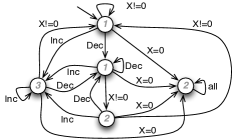
Figure 1: DPW (with priorities written in the states) for $\left[\operatorname{\Diamond}\operatorname{\Box}\neg Inc\ \wedge\ \operatorname{\Box}\operatorname{\Diamond}Dec\ \supset\ \operatorname{\Box}\operatorname{\Diamond}(X=0)\right]\supset\operatorname{\Diamond}(X=0)$.

Example (continued). We express $C_{X}$ in LTL. The constraint LTL formula $\Psi_{X}$ (over alphabet $\{X=0,X\neq 0\}\cup\{Inc,Dec\})$ is $\operatorname{\Diamond}\operatorname{\Box}\neg Inc\ \wedge\ \operatorname{\Box}\operatorname{\Diamond}Dec\ \supset\ \operatorname{\Box}\operatorname{\Diamond}(X=0)\,.$ Then, $mod(\Psi_{X})=C_{X}$. The resulting formula $\Phi\doteq\Psi_{X}\supset\operatorname{\Diamond}(X=0)$ generates a relatively small automaton: the DPW $A_{d}$ has 5 states and 3 priorities, see Figure 1. As a further example, consider the case of $N\in\mathbb{N}$ variables. Each variable $X_{i}$ has a formula $\Psi_{i}$ analogous to $\Psi_{X}$. Consider the constraint $\Psi=\wedge_{i}\Psi_{i}$. The above algorithm gives us, as worst-case, DPW for $\Phi\doteq\Psi\supset\operatorname{\Diamond}(X=0)$ of size $2^{2^{O(N)}}$ with $2^{O(N)}$ many priorities. However, analogously to Figure 1, there is a DPW of size $2^{O(N)}$ with $3$ priorities. ∎

5 Qualitative Numerical Problems

To concretize, we consider a simple but broad class of problems where generalized planning can be reduced to FOND planning. These problems have a set of non-negative numeric variables, that do not have to be integer, and standard boolean propositions and actions that can increase or decrease the value of the numeric variables non-deterministically. The general problem of stacking a block $x$ on a block $y$ in any blocks-world problem, with any number of blocks in any configuration, can be cast as a problem of this type. An abstraction of some of these problems appears in Srivastava et al. (2011b, 2015).

A qualitative numerical problem or QNP is a tuple $R_{V}=\langle F,Init,Act,G,V,Init_{V},INC,$ $DEC\rangle$ where the first four components define a STRIPS planning problem extended with atoms $X=0$ and $X>0$ for numerical variables $X$ in a set $V$, that may appear as action preconditions and goals, sets $Init_{V}(X)$ of possible initial values for each variable $X\in V$, and effect descriptors $Dec(X)$ and $Inc(X)$, with a semantics given by the functions $INC$ and $DEC$ that take a variable $X$, an action $a$, and a state $s$, and yield a subset $INC(X,a,s)$ and $DEC(X,a,s)$ of possible values $x^{\prime}$ of $X$ in the successor states. If these ranges contain a single number, the problem is deterministic, else it is non-deterministic. If $x$ is the value of $X$ in $s$, the only requirement is that for all $x^{\prime}\in DEC(x,a,s)$, $0\leq x^{\prime}\leq x$, and that for all $x^{\prime}\in INC(X,a,s)$, $x^{\prime}>x$ when $x=0$ and $x^{\prime}\geq x$ when $x>0$. All the propositions in $F$ are assumed to be observable, while for numerical variables $X$, only the booleans $X=0$ and $X>0$ are observable.

A QNP $R_{V}=\langle F,Init,Act,G,V,Init_{V},INC,$ $DEC\rangle$ represents a PONDP $P_{V}$ in syntactic form. If $s_{V}$ is a valuation over the variables in $V$, $s_{V}[X]$ is the value of $X$ in $s_{V}$, and $b[s_{V}]$ its boolean projection; i.e. $b[s_{V}][X]=0$ if $s_{V}[X]=0$ and $b[s_{V}][X]=1$ otherwise. The PONDP $P_{V}$ corresponds to the tuple $\langle S,I,\Omega,Act,T,A,obs,F\rangle$ where

1. $S$ is the set of valuations $\langle s_{F},s_{V}\rangle$ over the variables in $F$ and $V$ respectively,

2. $I$ is the set of pairs $\langle s_{F},s_{V}\rangle$ where $s_{F}$ is uniquely determined by $Init$ and $s_{V}[X]\in Init_{V}(X)$ for each $X\in V$,

3. $\Omega=\{\langle s_{F},b[s_{V}]\rangle:\langle s_{F},s_{V}\rangle\in S\}$,

4. $Act$ is the finite set of actions given,

5. $T\subseteq S$ is the set of states that satisfy the atoms in $G$,

6. $A(s)$ is the set of actions whose precondition are true in $s$,

7. $obs(s)=\langle s_{F},b[s_{V}]\rangle$ for $s=\langle s_{F},s_{V}\rangle$,

8. $F(a,s)$ for $s=\langle s_{F},s_{V}\rangle$ is the set of states $s^{\prime}=\langle s^{\prime}_{F},s^{\prime}_{V}\rangle$ where $s^{\prime}_{F}$ is the STRIPS successor of $a$ in $s$, and $s^{\prime}_{V}[X]$ is in $INC(X,a,s)$, $DEC(X,a,s)$, or $\{s_{V}[X]\}$ according to whether $a$ features an $Inc(X)$ effect, a $Dec(X)$ effect, or none.

An example is $R_{V}=\langle F,Init,Act,G,V,Init_{V},INC,$ $DEC\rangle$ where $F$ is empty, $V=\{X,Y\}$, $Init_{V}(X)=\{20\}$ and $Init_{V}(Y)=\{30\}$, the goal is $\{X=0,Y=0\}$, and $Act$ contains two actions: an action $a$ with effects $Dec(X)$ and $Inc(Y)$, and an action $b$ with effect $Dec(Y)$. The functions $INC$ always increases the value by 1 and $DEC$ decreases the value by 1 except when it is less than 1 when the value is decreased to $0$. A policy $\mu$ that solves $R_{V}$ is “do $a$ if $X>0$ and $Y=0$, and do $b$ if $Y>0$”. Simple variations of $R_{V}$ can be obtained by changing the initial situation, e.g., setting it to $Init_{V}(X)=[10,20]$ and $Init_{V}(Y)=[15,30]$, or the $INC$ and $DEC$ functions. For example, a variable $X$ can be set to increase or decrease any number between $0$ and $1$ as long as values do not become negative. The policy $\mu$ solves all these variations except for those where infinite sequences of decrements fail to drive a variable to zero. We rule out such QNPs by means of the following trajectory constraint:

Definition 11 (QNP Constraint).

The trajectory constraint $C_{X}$ for a numerical variable $X$ in a QNP excludes the trajectories that after a given time point contain a) an infinite number of actions with $Dec(X)$ effects, b) a finite number of actions with $Inc(X)$ effects, c) no state where $X=0$.

This is analogous to the LTL constraint in Section 4. The set of constraints $C_{X}$ for all variables $X\in V$ is denoted as $C_{V}$. We will be interested in solving QNPs $R_{V}$ given that the constraints $C_{V}$ hold. Moreover, as we have seen, there are policies that solve entire families of similar QNPs:

Definition 12 (Similar QNPs).

Two QNPs are similar if they only differ in the $INC$, $DEC$ or $Init_{V}$ functions, and for each variable $X$, $X=0$ is initially possible in one if it is initially possible in the other, and the same for $X>0$.

We want to obtain policies that solve whole classes of similar QNPs by solving a single abstract problem. For a QNP $R_{V}$, we define its syntactic projection as $R_{V}^{o}$:

Definition 13 (Syntactic Projection of QNPs).

If $R_{V}=\langle F,Init,Act,G,V,Init_{V},INC,DEC\rangle$ is a QNP, its syntactic projection is the non-deterministic (boolean) problem $R_{V}^{o}=\langle F^{\prime},Init^{\prime},Act^{\prime},G\rangle$, where

1. $F^{\prime}$ is $F$ with new atoms $X=0$ and $X>0$ added for each variable $X$; i.e. $F^{\prime}=F\cup\{X=0,X>0:X\in V\}$,

2. $Init^{\prime}$ is $Init$ and $X=0$ (resp. $X>0$) true iff $X>0$ (resp. $X=0$) is not initially possible in $Init_{V}$.

3. $Act^{\prime}$ is $Act$ but where in each action and for each variable $X$, the effect $Inc(X)$ is replaced by the atom $X>0$, and the effect $Dec(X)$ is replaced by the conditional effect “if $X>0$ then $X>0\,|\,X=0$”.

Recalling that $X>0$ is an abbreviation for $X\neq 0$, the atoms $X=0$ and $X>0$ are mutually exclusive. We refer to the action with non-deterministic effects in $R_{V}^{o}$ as the $Dec(X)$ actions as such actions have $Dec(X)$ effects in $R_{V}$. This convention is assumed when applying $C_{V}$ constraints to $R^{o}_{V}$. The syntactic projection $R_{V}^{o}$ denotes a FONDP that features multiple initial states when for some variable $X$, both $X=0$ and $X>0$ are possible in $Init_{V}$:

Theorem 14.

The FONDP denoted by $R_{V}^{o}$ is the observation projection of the class $\mathcal{R}_{V}$ made of all the PONDPs $R^{\prime}_{V}$ that are similar to $R_{V}$.

The generalization captured by Theorem 6 implies that:

Theorem 15 (QNP Generalization).

Let $\mu$ a policy that solves $R_{V}^{o}/C_{V}$; i.e. the FONDP denoted by $R_{V}^{o}$ given $C_{V}$. Then, $\mu$ solves $R^{\prime}_{V}/C_{V}$ for all QNPs $R^{\prime}_{V}$ similar to $R_{V}$.

In addition, the constraints $C_{V}$ are strong enough in QNPs for making the abstraction $R_{V}^{o}$ complete for the class of problems $\mathcal{R}_{V}$ similar to $R_{V}$:

Theorem 16 (QNP Completeness).

Let $\mu$ be a policy that solves the class of problems $\mathcal{R}_{V}$ made up of all the QNPs $R^{\prime}_{V}$ that are similar to $R_{V}$ given $C_{V}$. Then $\mu$ must solve the projection $R_{V}^{o}$ given $C_{V}$.

This is because the class $\mathcal{R}_{V}$ contains a problem $R^{*}_{V}$ where each variable $X$ has two possible values $X=0$ and $X=1$ such that the semantics of the $Dec(X)$ and $Inc(X)$ effects make $R^{*}_{V}$ equivalent to the projection $R^{o}_{V}$, with the valuations over the two-valued $X$ variables in correspondence with the boolean values $X=0$ and $X>0$ in $R_{V}^{o}$.

5.1 QNP Solving as FOND Planning

The syntactic projection $R_{V}^{o}$ of a QNP $R_{V}$ represents a FONDP with non-deterministic (boolean) effects $X>0\,|\,X=0$ for the actions in $R_{V}$ with $Dec(X)$ effects. It may appear from Theorem 15 that one could use off-the-shelf FOND planners for solving $R_{V}^{o}$ and hence for solving all QNPs similar to $R_{V}$. There is, however, an obstacle: the effects $X>0\,|\,X=0$ are not fair. Indeed, even executing forever only actions with $Dec(X)$ effects does not guarantee that eventually $X=0$ will be true. In order to use fair (strong cyclic) FOND planners off-the-shelf, we thus need to compile the FONDP $R^{o}_{V}$ given the constraints $C_{V}$ into a fair FONDP with no constraints.

For this, it is convenient to make two assumptions and to extend the problem $R_{V}$ with extra booleans and actions that do not affect the problem but provide us with handles in the projection. The assumptions are that actions with $Dec(X)$ effects have the (observable) precondition $X>0$, and more critically, that actions feature decrement effects for at most one variable. The new atoms are $q_{X}$, one for each variable $X\in V$, initially all false. The new actions for each variable $X$ in $V$ are $set(X)$ and $unset(X)$, the first with no precondition and effect $q_{X}$, the second with precondition $X=0$ and effect $\neg q_{X}$. Finally, preconditions $q_{X}$ are added to actions with effect $Dec(X)$ and precondition $\neg q_{X}$ to all actions with effect $Inc(X)$. Basically, $q_{X}$ is set in order to decrease the variable $X$ to zero. When $q_{X}$ is set, $X$ cannot be increased and $q_{X}$ can be unset only when $X=0$. We say that $R_{V}$ is closed when $R_{V}$ is extended in this way and complies with the assumptions above (and likewise for its projection $R_{V}^{o}$).

Theorem 17 (Generalization with FOND Planner).

$\mu$ is a fair solution to the FONDP $R^{o}_{V}$ for a closed QNP $R_{V}$ iff $\mu$ solves all QNPs that are similar to $R_{V}$ given the constraints $C_{V}$.

Sketch: We need to show that $\mu$ is a fair solution to $R^{o}_{V}$ iff $\mu$ solves $R^{o}_{V}/C_{V}$. The rest follows from Theorems 15 and 16. ($\Rightarrow$). If $\mu$ does not solve the FONDP $R^{o}_{V}$ given $C_{V}$, there must a $\mu$-trajectory $\tau$ that is not goal reaching but that satisfies $C_{V}$ and is not fair in $R^{o}_{V}$. Thus, there must be a subtrajectory $\langle s_{i},a_{i},\ldots,s_{i+m}\rangle$ that forms a loop with $s_{i+m}=s_{i}$, where no $s_{k}$ is a goal state, and 1) some $a_{k}$ has a $Dec(X)$ effect in $R_{V}$, and 2) $X>0$ is true in all $s_{k}$, $i\leq k\leq i+m$. 1) must be true as $\tau$ is not fair in $R^{o}_{V}$ and only actions with $Dec(X)$ actions in $R_{V}$ are not deterministic in $R_{V}^{o}$, and 2) must be true as, from the assumptions in $R_{V}$, $X=0$ needs to be achieved by an action that decrements $X$, in contradiction with the assumption that $\tau$ is not fair in $R_{V}^{o}$. Finally, since $\tau$ satisfies $C_{V}$, then it must contain infinite actions with $Inc(X)$ effects, but then the loop must feature $unset(X)$ actions with precondition $X=0$ in contradiction with 2. ($\Leftarrow$) If $\mu$ solves $R^{o}_{V}/C_{V}$ but $\mu$ is not a fair solution to $R^{o}_{V}$, then there must be an infinite $\mu$-trajectory $\tau$ that is not goal reaching and does not satisfy $C_{V}$, but which is fair in $R^{o}_{V}$. This means that there is a loop in $\tau$ with some $Dec(X)$ action, no $Inc(X)$ action, and where $X=0$ is false. But $\tau$ can’t then be fair in $R^{o}_{V}$.∎

6 Discussion

We have studied ways in which a (possibly infinite) set of problems with partial observations (PONDPs) that satisfy a set of trajectory constraints can all be solved by solving a single fully observable problem (FONDP) given by the common observation projection, augmented with the trajectory constraints. The trajectory constraints play a crucial role in adding enough expressive power to the observation projection. The single abstract problem can be solved with automata theoretic techniques typical of LTL synthesis when the trajectory constraints can be expressed in LTL, and in some cases, by more efficient FOND planners.

The class of qualitative numerical problems are related to those considered by Srivastava et al. [2011b; 2015] although the theoretical foundations are different. We obtain the FONDPs $R_{V}^{o}$ from an explicit observation projection, and rather than using FOND planners to provide fair solutions to $R_{V}^{o}$ that are then checked for termination, we look for strong solutions to $R_{V}^{o}$ given a set of explicit trajectory constraints $C_{V}$, and show that under some conditions, they can be obtained from fair solutions to a suitable transformed problem. It is also interesting to compare our work to the approach adopted to deal with the one-dimensional planning problems Hu and Levesque (2010); Hu and De Giacomo (2011). There we have infinitely many concrete problems that are all identical except for an unobservable parameter ranging over naturals that can only decrease. A technique for solving such generalized planning problems is based on defining one single abstract planning problem to solve that is “large enough” Hu and De Giacomo (2011). Here, instead, we would address such problems by considering a much smaller abstraction, the observation projection, but with trajectory constraints that capture that the hidden parameter can only decrease.

Our work is also relevant for planning under incomplete information. The prototypical example is the tree-chopping problem of felling a tree that requires an unknown/unobservable number of chops. This was studied by Sardiña et al. [2006], where, in our terminology, the authors analyse exactly the issue of losing the “global property” when passing to the “observation projection”. Finally, our approach can be seen as a concretization of insights by De Giacomo et al. [2016] where trace constraints are shown to be necessary for the belief-state construction to work on infinite domains.

References

- Belle and Levesque [2016] Vaishak Belle and Hector J. Levesque. Foundations for generalized planning in unbounded stochastic domains. In KR, pages 380–389, 2016.
- Bonet and Geffner [2009] Blai Bonet and Hector Geffner. Solving POMDPs: RTDP-Bel vs. Point-based Algorithms. In IJCAI, pages 1641–1646, 2009.
- Bonet and Geffner [2015] Blai Bonet and Hector Geffner. Policies that generalize: Solving many planning problems with the same policy. In IJCAI, pages 2798–2804, 2015.
- Bonet et al. [2009] Blai Bonet, Hector Palacios, and Hector Geffner. Automatic derivation of memoryless policies and finite-state controllers using classical planners. In ICAPS, 2009.
- Chatterjee and Chmelík [2015] Krishnendu Chatterjee and Martin Chmelík. POMDPs under probabilistic semantics. Artificial Intelligence, 221(C):46–72, 2015.
- Cimatti et al. [2003] Alessandro Cimatti, Marco Pistore, Marco Roveri, and Paolo Traverso. Weak, strong, and strong cyclic planning via symbolic model checking. Artificial Intelligence, 147(1-2):35–84, 2003.
- De Giacomo et al. [2016] Giuseppe De Giacomo, Aniello Murano, Sasha Rubin, and Antonio Di Stasio. Imperfect-information games and generalized planning. In IJCAI, pages 1037–1043, 2016.
- Gazen and Knoblock [1997] B. Cenk Gazen and Craig Knoblock. Combining the expressiveness of UCPOP with the efficiency of Graphplan. In ECP, pages 221–233, 1997.
- Hu and De Giacomo [2011] Yuxiao Hu and Giuseppe De Giacomo. Generalized planning: Synthesizing plans that work for multiple environments. In IJCAI, pages 918–923, 2011.
- Hu and Levesque [2010] Yuxiao Hu and Hector J. Levesque. A correctness result for reasoning about one-dimensional planning problems. In KR, 2010.
- Levesque [2005] Hector J. Levesque. Planning with loops. In IJCAI, pages 509–515, 2005.
- Piterman [2007] Nir Piterman. From nondeterministic büchi and Streett automata to deterministic parity automata. Log. Meth. in Comp. Sci., 3(3), 2007.
- Pnueli and Rosner [1989] Amir Pnueli and Roni Rosner. On the synthesis of an asynchronous reactive module. In ICALP, pages 652–671. 1989.
- Sardiña et al. [2006] Sebastian Sardiña, Giuseppe De Giacomo, Yves Lespérance, and Hector J. Levesque. On the limits of planning over belief states under strict uncertainty. In KR, pages 463–471, 2006.
- Srivastava et al. [2008] Siddharth Srivastava, Neil Immerman, and Shlomo Zilberstein. Learning generalized plans using abstract counting. In AAAI, 2008.
- Srivastava et al. [2011a] Siddharth Srivastava, Neil Immerman, and Shlomo Zilberstein. A new representation and associated algorithms for generalized planning. Artificial Intelligence, 175(2):615–647, 2011.
- Srivastava et al. [2011b] Siddharth Srivastava, Shlomo Zilberstein, Neil Immerman, and Hector Geffner. Qualitative numeric planning. In AAAI, 2011.
- Srivastava et al. [2015] Siddharth Srivastava, Shlomo Zilberstein, Abhishek Gupta, Pieter Abbeel, and Stuart Russell. Tractability of planning with loops. In AAAI, pages 3393–3401, 2015.
- Vardi and Wolper [1994] Moshe Y. Vardi and Pierre Wolper. Reasoning about infinite computations. I&C, 115(1):1–37, 1994.
- Zielonka [1998] Wicslaw Zielonka. Infinite games on finitely coloured graphs with applications to automata on infinite trees. Theor. Comput. Sci., 200(1-2):135–183, 1998.