Compound vectors of subordinators and their associated positive Lévy copulas

Abstract

Lévy copulas are an important tool which can be used to build dependent Lévy processes. In a classical setting, they have been used to model financial applications. In a Bayesian framework they have been employed to introduce dependent nonparametric priors which allow to model heterogeneous data. This paper focuses on introducing a new class of Lévy copulas based on a class of subordinators recently appeared in the literature, called Compound Random Measures. The well-known Clayton Lévy copula is a special case of this new class. Furthermore, we provide some novel results about the underlying vector of subordinators such as a series representation and relevant moments. The article concludes with an application to a Danish fire dataset.

Keywords: Dependent Completely Random Measures, Lévy processes, Clayton Lévy copulas.

1 Introduction

Vectors of subordinators, namely a real valued non-decreasing stochastic process with independent increments, are an important class of processes which have been used for the modeling of data arising from multiple components. For example, Yuen et al. (2016) solve the ruin problem for a bivariate Poisson process, Semeraro (2008) uses a vector of Gamma processes to construct a multivariate variance gamma model for financial applications and Esmaeili and Klüppelberg (2010) perform parameter estimation for bivariate compound Poisson processes which they apply to an insurance dataset. Esmaeili and Klüppelberg (2011) focus on parameter estimation for a vector of stable processes, Jiang et al. (2019) deal with a vector of gamma processes, and Esmaeili and Klüppelberg (2013) present a two-step estimation method for general multivariate Lévy processes. In the context of Bayesian non-parametric statistics, vectors of subordinators have been used to construct dependent priors to model heterogeneous data; the celebrated Dirichlet Process, introduced in Ferguson (1973), can be seen as a normalized Gamma subordinator. In the context of survival analysis, Doksum (1974) employs 1-dimensional subordinators to build the so-called neutral to the right priors. More complex Bayesian nonparametric priors based on vectors of subordinators have been proposed such as, the vectors of dependent random measures in Lijoi et al. (2014), obtained through entrywise normalization of a vector of subordinators or the multivariate survival priors in Epifani and Lijoi (2010) and Riva-Palacio and Leisen (2018a) which use vectors of subordinators to extend the neutral to the right priors into a partially exchangeable setting. Ishwaran and Zarepour (2009) proposed a vector of generalized gamma processes and Leisen and Lijoi (2011) proposed a vector of Poisson-Dirichlet processes constructed using a vector of stable processes. More recently Camerlenghi et al. (2019) and Camerlenghi et al. (2020) proposed flexible dependent priors to model data heterogeneity.

The dependence structure for the entries of a vector of subordinators is particularly important for application purposes. In this context, the main approach to model the dependence is the one of Lévy copulas where in analogy with distributional copulas, see Nelsen (2007), the marginal behavior of the vector of subordinators can be decoupled from the dependence structure. As highlighted in Tankov (2016), Lévy copulas have found important applications in statistical inference for vectors of Lévy processes, the study of multivariate regular variation and risk management applications. In Section 4 we will focus on parameter inference as discussed in Esmaeili and Klüppelberg (2010), Esmaeili and Klüppelberg (2011) and Esmaeili and Klüppelberg (2013).

In a Bayesian non-parametric framework Griffin and Leisen (2017) introduced a class of vector of subordinators which relies on a one-dimensional subordinator and a $d$-variate probability distribution in $\left(\mathbb{R}^{+}\right)^{d}$ to determine the corresponding vector. Although their construction relies on the concept of completely random measures, see Kingman (1967), in this work we use the equivalent setting of subordinators and present new results regarding these vectors which henceforward, we call compound vectors of subordinators. In particular, we present a novel compound vector of subordinators which exhibits asymmetry in its related Lévy copula. We provide a series representation for compound vectors of subordinators and exemplify its use for simulation purposes. We also provide a new criteria for compound vector of subordinators to be well defined and give formulas for the associated fractional moments of order less than one, means, variances and covariances. Griffin and Leisen (2017) showed the structure of the Lévy copula associated to a compound vector of subordinator in a particular case, namely when what they call the score distribution in their construction has independent and identically distributed marginal distributions; further exploration of the Lévy copula structure was not performed. In the present work we explore the general Lévy copula structure associated to a vector of compound subordinators. On the other hand, we give a tractable example of an asymmetric family of Lévy copulas arising from a compound vector of subordinators. This new family is interesting as it contains the symmetric Clayton Lévy copula as a particular case and preserves the behavior of a parameter modulating between indepence and complete dependence while allowing an extra parameter $\boldsymbol{\alpha}$ to modulate asymmetry. In a similar fashion to Esmaeili and Klüppelberg (2010), we show the use of such new family for the modelling of a bivariate compound Poisson process and the related parameter inference. A simulation study for a vector of stable processes and a real data study pertaining insurance are performed. We conclude that broader classes of Lévy copulas are needed and the compound vector of subordinators approach is a valid and tractable way to do so.

The outline of the paper is the following. Section 2 introduces vectors of dependent subordinators and Lévy copulas. Section 3 and Section 4 are devoted to illustrate the main results of the paper. Section 5 includes application of the new model to simulated and real data sets. Section 6 concludes with a discussion. All the proofs of the results are in the Appendix.

2 Preliminaries

This section is devoted to introduce some preliminary notions about vectors of subordinators and Lévy copulas.

Definition 1.

We say that $\boldsymbol{Y}=(Y_{1},\ldots,Y_{d})$, $d\in\mathbb{N},$ is a $d$-variate vector of positive jump Lévy processes if for $t>0$, $\boldsymbol{\lambda}\in(\mathbb{R}^{+})^{d}$

$$\mathbb{E}\!\left[e^{-\lambda_{1}Y_{1}(t)-\ldots-\lambda_{d}Y_{d}(t)}\right] =e^{-\int_{(\mathbb{R}^{+})^{d}\times[0,t]}(1-e^{-\lambda_{1}s_{1}-\ldots-\lambda_{d}s_{d}})\nu(\mathrm{d}s_{1},\ldots,\mathrm{d}s_{d},\mathrm{d}x)}$$

$$=e^{-\int_{(\mathbb{R}^{+})^{d}\times[0,t]}(1-e^{-\langle\boldsymbol{\lambda}\,,\,\boldsymbol{s}\rangle})\nu(\mathrm{d}\boldsymbol{s},\mathrm{d}x)},$$

with $\nu$ a measure in $\left((\mathbb{R}^{+})^{d+1},\mathcal{B}\left((\mathbb{R}^{+})^{d+1}\right)\right)$ such that

$$\int_{(\mathbb{R}^{+})^{d}\times\mathbb{R}^{+}}\min\left\{1,\|\boldsymbol{s}\|\right\}\nu(\mathrm{d}\boldsymbol{s},\mathrm{d}x)<\infty.$$ (1)

We call $\nu$ the Lévy intensity of $\boldsymbol{Y}$.

In the following we refer to the stochastic process defined above as a vector of subordinators. We say that a Lévy intensity is homogeneous if

$$\nu(\mathrm{d}\boldsymbol{s},\mathrm{d}x)=\rho(\mathrm{d}\boldsymbol{s})\alpha(\mathrm{d}x).$$

We define the Laplace exponent of an univariate subordinator, see Sato et al. (1999) for details.

Definition 2.

Let $\nu$ be a Lévy intensity with $d=1$ and associated subordinator $Y$. We say that the Laplace exponent of $\nu$ is

$$\psi_{t}(\lambda)=\int_{0}^{t}\int_{0}^{\infty}(1-e^{-\lambda s})\nu(\mathrm{d}s,\mathrm{d}x)=-\log\left(\mathbb{E}\!\left[e^{-\lambda Y(t)}\right]\right).$$

The tail integral of a vector of subordinators plays an important role in the results displayed in Section 3 and 4. It is defined as follows.

Definition 3.

Let $\boldsymbol{Y}$ be a vector of subordinators with homogeneous Lévy intensity $\rho$. Its associated tail integral is defined as

$$U(\boldsymbol{y})=\int_{[y_{1},\infty)\times\ldots\times[y_{d},\infty)}\rho(\mathrm{d}\boldsymbol{s}).$$ (2)

The marginal tail integrals associated to $U(\boldsymbol{y})$ are given by

$$U_{i}(y)=U(y_{1}^{(i)},\ldots,y_{i-1}^{(i)},y,y_{i+1}^{(i)},\ldots,y_{d}^{(i)}),$$

where $y_{1}^{(i)}=\cdots=y_{i-1}^{(i)}=y_{i+1}^{(i)},=\ldots=y_{d}^{(i)}=0$ for $i\in\{1,\ldots,d\}$.

Given a vector of subordinators, $\boldsymbol{Y}=(Y_{1},\ldots,Y_{d})$, there exist collections of random elements $\{W_{1,i}\}_{i=1}^{\infty},\ldots,\{W_{d,i}\}_{i=1}^{\infty}$ and $\{V_{i}\}_{i=1}^{\infty}$ such that

$$\left(Y_{1}(t),\ldots,Y_{d}(t)\right) \stackrel{{\scriptstyle\text{a.s.}}}{{=}}\left(\sum_{i=1}^{\infty}W_{1,i}\mathbbm{1}_{\left\{V_{i}\leq t\right\}},\ldots,\sum_{i=1}^{\infty}W_{d,i}\mathbbm{1}_{\left\{V_{i}\leq t\right\}}\right).$$ (3)

For a full review of vectors of subordinators see Cont and Tankov (2004). The construction in Griffin and Leisen (2017) for vectors of completely random measures can be set in the context of vectors of subordinators as follows.

Definition 4.

Let $h$ be a $d-$variate probability density function and $\nu^{\star}$ a univariate Lévy intensity. We say that a vector of subordinators $\boldsymbol{Y}$ is a $d-$variate compound vector of subordinators with score distribution $h$ and directing Lévy measure $\nu^{\star}$ if it has a $d-$variate Lévy intensity given by

$$\nu(\mathrm{d}\boldsymbol{s},\mathrm{d}x)=\int z^{-d}h(s_{1}/z,\ldots,s_{d}/z)\nu^{\star}(\mathrm{d}z,\mathrm{d}x)\mathrm{d}\boldsymbol{s}.$$

If the directing Lévy measure is homogeneous, $\nu^{\star}(\mathrm{d}\boldsymbol{s},\mathrm{d}x)=\rho^{\star}(\mathrm{d}\boldsymbol{s})\alpha(\mathrm{d}x)$, then $\nu(\mathrm{d}\boldsymbol{s},\mathrm{d}x)=\rho(\mathrm{d}\boldsymbol{s})\alpha(\mathrm{d}x)$ with

$$\rho(\mathrm{d}\boldsymbol{s})=\int z^{-d}h(s_{1}/z,\ldots,s_{d}/z)\rho^{\star}(\mathrm{d}z)\mathrm{d}\boldsymbol{s}.$$

In the next result we present what will be the running working example of this work. In particular, we restrict ourselves to the $2$-dimensional vector of subordinators setting for illustration purposes.

Theorem 1.

Let $\sigma\in(0,1)$, and $\alpha_{1},\beta_{1},\alpha_{2},\beta_{2}>0$. If the score distribution is given by

$$h(y_{1},y_{2})=\frac{\beta_{1}^{\alpha_{1}}\beta_{2}^{\alpha_{2}}}{\Gamma(\alpha_{1})\Gamma(\alpha_{2})}y_{1}^{\alpha_{1}-1}e^{-\beta_{1}y_{1}}y_{2}^{\alpha_{2}-1}e^{-\beta_{2}y_{2}},$$

i.e. the score distribution is given by independent $\text{Gamma}(\alpha_{1},\beta_{1})$, $\text{Gamma}(\alpha_{2},\beta_{2})$ distributions, and the directing Lévy measure has intensity

$$\rho^{\star}(z)=\sigma Kz^{-\sigma-1},$$

i.e. a $\sigma$-stable intensity with proportionality parameter $K=\sigma/\Gamma(1-\sigma)$. Then the corresponding compound vector of subordinators has a bivariate Lévy intensity given by

$$\rho_{\sigma,K,\boldsymbol{\alpha},\boldsymbol{\beta}}(\mathrm{d}s_{1},\mathrm{d}s_{2})=\frac{\sigma K\beta_{1}^{\alpha_{1}}\beta_{2}^{\alpha_{2}}\Gamma(\alpha_{1}+\alpha_{2}+\sigma)s_{1}^{\alpha_{1}-1}s_{2}^{\alpha_{2}-1}}{\Gamma(\alpha_{1})\Gamma(\alpha_{2})(\beta_{1}s_{1}+\beta_{2}s_{2})^{\alpha_{1}+\alpha_{2}+\sigma}}\mathrm{d}s_{1}\mathrm{d}s_{2},$$ (4)

and has $\sigma$-stable marginals with proportionality parameters

$$K_{i}=\frac{K\beta_{i}^{-\sigma}\Gamma(\alpha_{i}+\sigma)}{\Gamma(\alpha_{i})},$$

corresponding to each dimension $i\in\left\{1,2\right\}$.

The above result is a generalization of Corollary 1 in Griffin and Leisen (2017) where $\alpha_{1}=\alpha_{2}$ and $\beta_{1}=\beta_{2}=1$ was considered. Furthermore, the case $\alpha_{1}=\alpha_{2}=\beta_{1}=\beta_{2}=1$ was considered by Epifani and Lijoi (2010) and Leisen and Lijoi (2011) who link it to Clayton Lévy copulas, to be discussed next. This simple example exhibits the possibility to tractably link compound vectors of subordinators to Lévy copulas. In Griffin and Leisen (2017) only symmetric multivariate Lévy intensities where considered, however departure from such symmetry is of importance for modelling purposes as will be showed in Section 5. In Section 4 we will present the asymmetric Lévy copula associated to the particular compound vector of subordinators above.

A popular approach for modelling the dependence structure of vectors of subordinators is given by Lévy copulas.

Definition 5.

A $d-$variate positive Lévy copula is a function $\mathcal{C}(s_{1},\ldots,s_{d}):[0,\infty]^{d}\rightarrow[0,\infty]$ which satisfies

1. $\mathcal{C}(s_{1},\ldots,s_{d})<\infty$ for $(s_{1},\ldots,s_{d})\neq(\infty,\ldots,\infty)$.

2. $\mathcal{C}$ is $d-$increasing.

3. $\mathcal{C}(s_{1},\ldots,s_{d})=0$ if $s_{k}=0$ for any $k\in\{1,\ldots,d\}$

4. $\mathcal{C}(y_{1}^{(k)},\dots,y_{k-1}^{(k)},s,y_{k+1}^{(k)},\dots,y_{d}^{(k)})=s$ for $k\in\{1,\dots,d\}$, $s\in\mathbb{R}^{+}$, where $y_{1}^{(k)}=\dots=y_{k-1}^{(k)}=y_{k+1}^{(k)}=\dots=y_{d}^{(k)}=\infty$.

Such Lévy copulas can be linked to a vector of subordinators via the following theorem.

Theorem 2 (Cont and Tankov (2004)).

(Sklar’s Theorem for tail integrals and Lévy copulas) Let $U$ be a $d$-variate tail integral with margins $U_{1},\ldots,U_{d}$ then there exists a Lévy copula $\mathcal{C}$ such that

$$U(\boldsymbol{y})=\mathcal{C}(U_{1}(y_{1}),\ldots,U_{d}(y_{d})).$$

If $\{U_{i}\}_{i=1}^{d}$ are continuous $\mathcal{C}$ is unique, otherwise it is unique in $\text{Ran}(U_{1})\times\ldots\times\text{Ran}(U_{d})$.

For a proof see Theorem 5.3 in Cont and Tankov (2004). If the Lévy copula is smooth enough then from Theorem 2 and the definition of the tail integral we have that the underlying multivariate Lévy intensity can be expressed as

$$\rho(\boldsymbol{s})={\left.\kern-1.2pt\frac{\partial^{d}}{\partial u_{1}\cdots\partial u_{d}}\mathcal{C}(\boldsymbol{u})\vphantom{\big{|}}\right|_{u_{1}=U_{1}(s_{1}),\cdots,u_{d}=U_{d}(s_{d})}}\rho_{1}(s_{1})\cdots\rho_{d}(s_{d}),$$ (5)

where $\rho_{i}$, $i\in\{1,\ldots,d\}$, are the corresponding marginal Lévy intensities associated to the tail integrals $U_{1},\ldots,U_{d}$. Furthermore if $\mathcal{C}$ is a two dimensional Lévy copula and $\{\left(W_{1,i},W_{2,i}\right)\}_{i=1}^{\infty}$ are the random weights of a series representation for the associated vector of subordinators, equation (3), then the law of $S_{1,i}=U_{1}\left(W_{1,i}\right)$ conditioned on $S_{2,i}=U_{2}\left(W_{2,i}\right)=s_{2}\in\mathbb{R}^{+}\setminus\{0\}$ is given by the distribution function

$$\hat{F}_{S_{1}|S_{2}=s_{2}}(s_{1}) =\frac{\partial}{\partial s_{2}}\mathcal{C}(s_{1},s_{2}),$$ (6)

and the law of $S_{2,i}=U_{2}\left(W_{2,i}\right)$ conditioned on $S_{1,i}=U_{1}\left(W_{1,i}\right)=s_{1}\in\mathbb{R}^{+}\setminus\{0\}$ is given by the distribution function

$$\hat{F}_{S_{2}|S_{1}=s_{1}}(s_{2}) =\frac{\partial}{\partial s_{1}}\mathcal{C}(s_{1},s_{2});$$ (7)

see Theorem 6.3 in Cont and Tankov (2004) for a proof. Some examples of $d$-variate positive Lévy copulas are the following:

Example 1.

Independence Lévy copula.

$$\mathcal{C}_{\perp}(s_{1},\ldots,s_{d})=\sum_{i=1}^{d}s_{i}\prod_{j\neq i}\mathbbm{1}_{\{s_{j}=\infty\}}.$$

In this case the subordinators $Y_{1},\ldots,Y_{d}$ are pairwise independent.

Example 2.

Complete dependence Lévy copula.

$$\mathcal{C}_{||}(s_{1},,\ldots,s_{d})=\min\{s_{1},\ldots,s_{d}\}.$$

In this case the subordinators $Y_{1},\ldots,Y_{d}$ are completely dependent in the sense that the vector of jump weights for the associated series representation, (3), $\left\{\left(W_{1,i},\ldots,W_{d,i}\right)\right\}_{i=1}^{\infty}$, are in a set $S$ such that whenever $\boldsymbol{v},\boldsymbol{u}\in S$ then either $v_{j}<u_{j}$ or $u_{j}<v_{j}$ for all $j\in\{1,\dots,d\}$.

The following Lévy copula example is of interest in the literature as it has as limiting cases the independence and complete dependence examples above.

Example 3.

Clayton Lévy copula.

$$\mathcal{C}_{\theta}(s_{1},\ldots,s_{d})=\left(s_{1}^{-\theta}+\ldots+s_{d}^{-\theta}\right)^{-1/\theta};\quad\theta>0.$$

The parameter $\theta$ in the Clayton Lévy copula allows us to modulate between the independence and complete dependence cases as

$$\lim_{\theta\to 0}\mathcal{C}_{\theta}(s_{1},\ldots,s_{d})=\mathcal{C}_{\perp}(s_{1},\ldots,s_{d})$$

and

$$\lim_{\theta\to\infty}\mathcal{C}_{\theta}(s_{1},\ldots,s_{d})=\mathcal{C}_{||}(s_{1},,\ldots,s_{d}).$$

Such example is the Lévy copula analogue of the distributional Clayton copula which also modulates between independence and complete dependence cases for multivariate probability distributions, see Nelsen (2007). We observe that the Clayton Lévy copula is symmmetric which for real data applications can be too strong a constraint. For a full review of Lévy copulas see Cont and Tankov (2004).

3 Results for compound vectors of subordinators

This section provides general results for compound subordinators. In particular, we provide a series representation, conditions for the vector to be well posed and expressions for the mean, variance and correlation of the process. In the first result we provide a representation with the structure displayed in equation (3).

Theorem 3.

Let $\boldsymbol{Y}=(Y_{1},\ldots,Y_{d})$ be a compound subordinator given by a score distribution $h$ and directing Lévy measure $\nu^{\star}$ with associated univariate subordinator $Y^{\star}$. Then for $\bm{t}\in\left(\mathbb{R}^{+}\right)^{d}$

$$\boldsymbol{Y}(\boldsymbol{t}) =\left(Y_{1}(t_{1}),\ldots,Y_{d}(t_{d})\right)\stackrel{{\scriptstyle\text{a.s.}}}{{=}}\left(\sum_{i=1}^{\infty}M_{1,i}W_{i}\mathbbm{1}_{\left\{V_{i}\leq t_{1}\right\}},\ldots,\sum_{i=1}^{\infty}M_{d,i}W_{i}\mathbbm{1}_{\left\{V_{i}\leq t_{d}\right\}}\right),$$

where

$$Y^{\star}(t)\stackrel{{\scriptstyle\text{a.s.}}}{{=}}\sum_{i=1}^{\infty}W_{i}\mathbbm{1}_{\left\{V_{i}\leq t\right\}}$$

with $t\in\mathbb{R}^{+}$, and

$$(M_{1,i},\ldots,M_{d,i})\stackrel{{\scriptstyle\text{i.i.d.}}}{{\sim}}h.$$

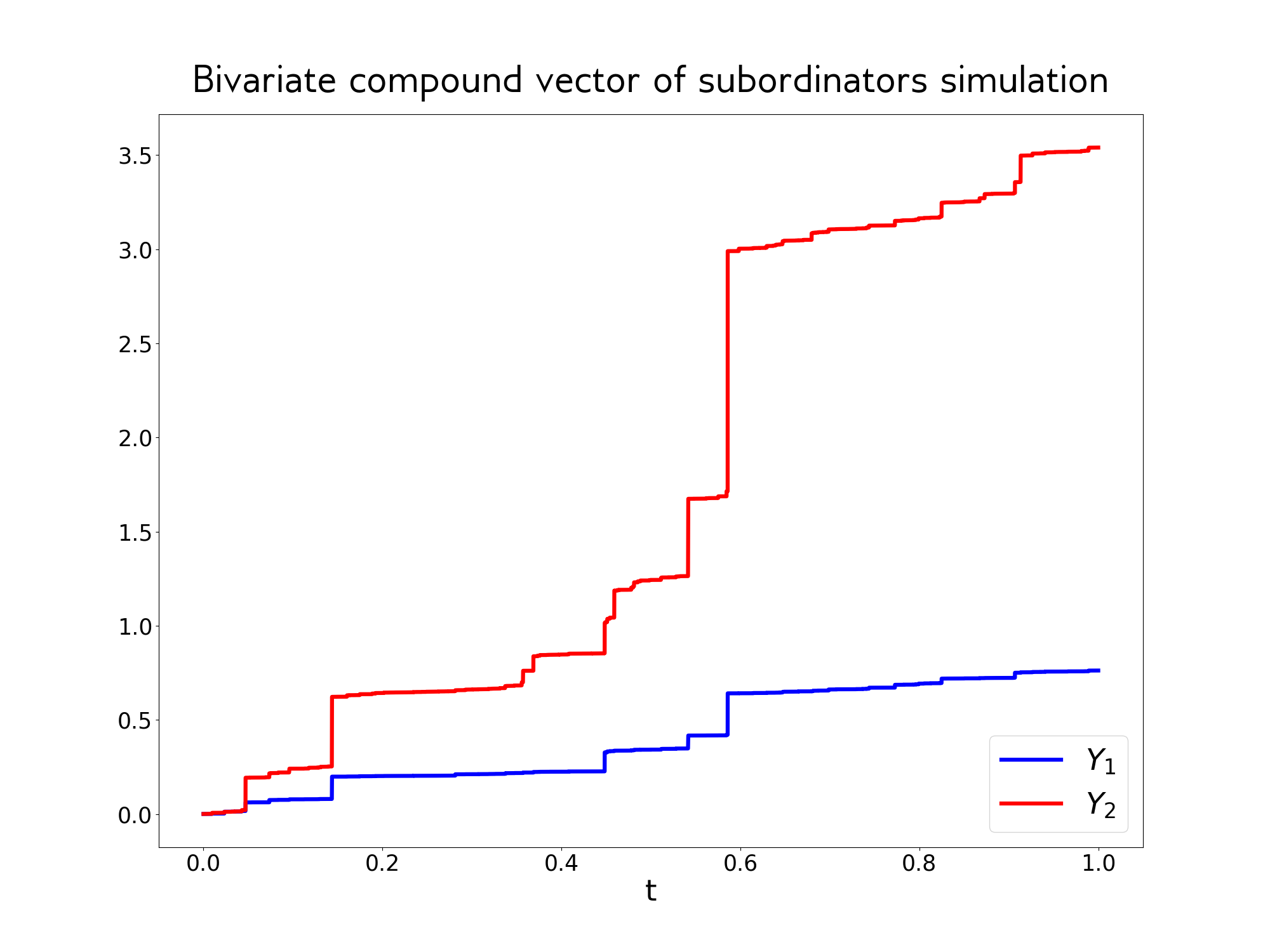
Figure 1: Simulation in $[0,1]$ of working example compound vector of subrodinators $\boldsymbol{Y}=(Y_{1},Y_{2})$ as in Theorem 1 with $\alpha_{1}=1$, $\beta_{1}=2$, $\alpha_{2}=10$, $\beta_{2}=5$, $\sigma=0.5$ and $K=1$; obtained by the series representation (8) with weights associated to the directing Lévy measure restricted to be greater than $\tau=10^{-6}$.

The above result is useful for computational purposes and provides a deeper understanding of the discrete structure of the process. In particular, if a series representation of the subordinator associated to the directing Lévy measure is available then a simulation algorithm for the compound vector of subordinators can be constructed. Let $Y^{\star}$ and $U^{\star}$ be, respectively, the subordinator and tail integral associated to a directing Lévy measure $\nu^{\star}$ which is absolutely continuous with respect to Lebesgue measure, and $(U^{\star})^{-1}$ be the inverse of the tail integral. A popular series representation is given by the Ferguson-Klass algorithm as it follows.

Theorem 4.

Let $\left\{U_{i}\right\}_{i=1}^{\infty}$ be i.i.d uniform random variables in $[0,1]$, $\left\{T_{i}\right\}_{i=1}^{\infty}$ be i.i.d. standard exponential random variables and $\Gamma_{k}=\sum_{i=1}^{k}T_{i}$. Then

$$Y^{\star}(t)=\sum_{i=1}^{\infty}(U^{\star})^{-1}(\Gamma_{i})\mathbbm{1}_{\left\{U_{i}\leq t\right\}},$$

for $t\in[0,1]$.

If the above series representation is truncated at an index $k$ such that $(U^{\star})^{-1}(\Gamma_{k})<\tau$ then the missing jump weights on the series are a.s. less than $\tau$. Letting $h$ be a score distribution and $\left\{(M_{1,i},\ldots,M_{d,i})\right\}_{i=1}^{k}\stackrel{{\scriptstyle\text{i.i.d.}}}{{\sim}}h$ then each entry of the compound vector of subordinators associated to $\nu^{\star}$ and $h$ has a truncated series approximation

$$Y_{j}(t)\approx\sum_{i=1}^{k}M_{j,i}(U^{\star})^{-1}(\Gamma_{i})\mathbbm{1}_{\left\{U_{i}\leq t\right\}},$$ (8)

for $t\in[0,1]$ and $j\in\left\{1,\ldots,d\right\}$. Where the missing jump weights for entry $j$ are randomly bounded to be less than $\min\left\{M_{j,1},\ldots M_{j,k}\right\}\tau$. We refer to Rosinski (2001) for a full review of series representations for Lévy processes and to Cont and Tankov (2004) for a review of simulation algorithms for Lévy processes. The inverse of the tail integral for a $\sigma$-stable Lévy measure is readily available, see the proof of Theorem 1 for details, so we can apply the Ferguson-Klass algorithm. In Figure 1 we simulate a trivariate vector of subordinators given by our working example in Theorem 1. The next result provides practical condition to check if a compound vector of subordinators is well posed.

Theorem 5.

Let $\nu^{\star}$ be a Lévy measure and $h$ a $d$-variate score distribution such that if $(W_{1},\ldots,W_{d})\sim h$ then $\mathbb{E}\!\left[W_{i}\right]<\infty$ $\forall i\in\{1,\ldots,d\}$. Then the compound vector of subordinators with directing Lévy measure $\nu^{\star}$ and score distribution $h$ has a Lévy intensity which satisfies condition (1).

The above theorem improves the result presented in Riva-Palacio and Leisen (2018b) by providing straightforward conditions to test if a vector of compound subordinators is well defined. For instance, our working example in Theorem 1, with score distribution given by independent marginal Gamma distributions, can be readily seen to be well posed as Gamma random variables always have finite mean.
This section concludes with a result which can be useful for modelling purposes and to understand the behavior of the process. Let $\psi_{t}$ be a Laplace exponent, we denote with $\psi_{t}^{\prime}(0)={\left.\kern-1.2pt\frac{\mathrm{d}}{\mathrm{d}\lambda}\psi_{t}(\lambda)\vphantom{\big{|}}\right|_{\lambda=0}}$ the first derivative evaluated in $0$. The moments of a compound vector of subordinators are given in the next result.

Theorem 6.

Let $\boldsymbol{Y}$ be a vector of compound subordinators with score distribution $h$ and directing Lévy measure $\nu^{\star}$ with Laplace exponent $\psi_{t}^{\star}$ such that $\left(\psi_{t}^{\star}\right)^{\prime}(0)$ and $\left(\psi_{t}^{\star}\right)^{\prime\prime}(0)$ exist $\forall t>0$; then

$$\mathbb{E}\!\left[Y_{i}(t)\right] =(\psi_{t}^{\star})^{\prime}(0)\mathbb{E}\!\left[W_{i}\right],$$

$$\mathbb{E}\!\left[\left(Y_{i}(t)\right)^{p}\right] =\frac{p}{\Gamma(1-p)}\int_{0}^{\infty}\frac{1-e^{-\mathbb{E}\!\left[\psi^{\star}_{t}(uW_{i})\right]}}{u^{p+1}}\mathrm{d}u\text{ for }p\in(0,1),$$

$$\text{Var}\!\left(Y_{i}(t)\right) =-(\psi_{t}^{\star})^{\prime\prime}(0)\mathbb{E}\!\left[W_{i}^{2}\right],$$

$$Cov\!\left(Y_{i}(t),Y_{j}(t)\right) =-(\psi_{t}^{\star})^{\prime\prime}(0)\mathbb{E}\!\left[W_{i}W_{j}\right],$$

$$Cor\!\left(Y_{i}(t),Y_{j}(t)\right) =\frac{\mathbb{E}\!\left[W_{i}W_{j}\right]}{\sqrt{\mathbb{E}\!\left[W_{i}^{2}\right]\mathbb{E}\!\left[W_{j}^{2}\right]}},$$

where $(W_{1},\ldots,W_{d})\sim h$ and $i,j\in\{1,\ldots,d\}$, $i\neq j$.

The fractional moment formula of order $p\in(0,1)$ in the previous theorem is useful when dealing with $\sigma$-stable processes which do not have finite moments for $p\geq\sigma$. In our working example, the directing Lévy measure is $\sigma$-stable which can be seen to have Laplace exponent $\psi^{\star}_{t}(\lambda)=K\lambda^{\sigma}$ and $W_{i}\sim\text{Gamma}(\alpha_{i},\beta_{i})$, which satisfies $\mathbb{E}\!\left[W_{i}^{\sigma}\right]=\frac{\Gamma(\alpha_{i}+\sigma)}{\Gamma(\alpha_{i})\beta_{i}^{\sigma}}$ with $i\in\left\{1,2\right\}$. So for $p<\sigma$ using the previous theorem and integrating by parts we have that

$$\mathbb{E}\!\left[\left(Y_{i}(t)\right)^{p}\right] =\frac{p}{\Gamma(1-p)}\int_{0}^{\infty}\frac{1-e^{-\mathbb{E}\!\left[tK(uW_{i})^{\sigma}\right]}}{u^{p+1}}\mathrm{d}u=\frac{K\mathbb{E}\!\left[W_{i}^{\sigma}\right]}{\Gamma(1-p)}\int_{0}^{\infty}\sigma e^{-tK\mathbb{E}\!\left[W_{i}^{\sigma}\right]u^{\sigma}}u^{\sigma-p-1}\mathrm{d}u$$

$$=\frac{K\mathbb{E}\!\left[W_{i}^{\sigma}\right]}{\Gamma(1-p)}\int_{0}^{\infty}\sigma e^{-tK\mathbb{E}\!\left[W_{i}^{\sigma}\right]u}u^{1-\frac{p}{\sigma}-1}\mathrm{d}u=\frac{\left(tK\mathbb{E}\!\left[W_{i}^{\sigma}\right]\right)^{\frac{p}{\sigma}}\Gamma(1-\frac{p}{\sigma})}{\Gamma(1-p)},$$

which agrees with Theorem 1 and the fractional moment formula for $\sigma$-stable processes, see Sato et al. (1999) p. 162 or set $W_{i}\stackrel{{\scriptstyle\text{a.s.}}}{{=}}1$ in the previous calculation. In Figure 2 we plot fractional moments for the working example of Theorem 1.

Figure 2: Fractional moments of order $p=0.49$ for working example compound vector of subrodinators $\boldsymbol{Y}=(Y_{1},Y_{2})$ as in Theorem 1 with $\alpha_{1}=1$, $\beta_{1}=2$, $\alpha_{2}=10$, $\beta_{2}=5$, $\sigma=0.5$ and $K=1$ with $t\in[0,1]$.

4 Positive Lévy copulas from compound vectors of subordinators

In this section we provide a new family of Lévy copulas, which has the Clayton Lévy copula in Example 3 as a particular case, and give a general formula for the Lévy copula associated to a compound vector of subordinators.

4.1 $(\alpha_{1},\alpha_{2})$-Clayton Lévy copulas

We present the family of $(\alpha_{1},\alpha_{2})$-Clayton Lévy copulas. This new family allows for asymmetry of the Lévy copulas and has two extra parameters with respect to the Clayton Lévy copula, which offer more flexibility in modelling. We derive the new family by considering the Lévy Copula associated to the compound vector of subordinators in Theorem 1. Let the regularized incomplete beta function be given by

$$I(x,\alpha,\beta)=\frac{\Gamma(a+b)}{\Gamma(a)\Gamma(b)}\int_{0}^{x}z^{\alpha-1}(1-z)^{\beta-1}\mathrm{d}z.$$

The next theorem provides the Lévy copula associated to the Lévy intensity in equation (4).

Theorem 7.

Let $\sigma\in(0,1)$, $K>0$ and $\boldsymbol{\alpha}=(\alpha_{1},\alpha_{2})$, $\boldsymbol{\beta}=(\beta_{1},\beta_{2})$ have positive non-zero entries. Then

1. The Lévy copula associated to $\rho_{\sigma,K,\boldsymbol{\alpha},\boldsymbol{\beta}}$ in Theorem 1 is given by

   $$\mathcal{C}_{\sigma,\boldsymbol{\alpha}}(s_{1},s_{2}) =s_{1}\,I\left(\frac{\left(\frac{\Gamma(\alpha_{1}+\sigma)}{\Gamma(\alpha_{1})s_{1}}\right)^{\frac{1}{\sigma}}}{\left(\frac{\Gamma(\alpha_{1}+\sigma)}{\Gamma(\alpha_{1})s_{1}}\right)^{\frac{1}{\sigma}}+\left(\frac{\Gamma(\alpha_{2}+\sigma)}{\Gamma(\alpha_{2})s_{2}}\right)^{\frac{1}{\sigma}}},\alpha_{1}+\sigma,\alpha_{2}\right)$$

   $$\hphantom{=}+s_{2}\,I\left(\frac{\left(\frac{\Gamma(\alpha_{2}+\sigma)}{\Gamma(\alpha_{2})s_{2}}\right)^{\frac{1}{\sigma}}}{\left(\frac{\Gamma(\alpha_{1}+\sigma)}{\Gamma(\alpha_{1})s_{1}}\right)^{\frac{1}{\sigma}}+\left(\frac{\Gamma(\alpha_{2}+\sigma)}{\Gamma(\alpha_{2})s_{2}}\right)^{\frac{1}{\sigma}}},\alpha_{2}+\sigma,\alpha_{1}\right).$$

2. Furthermore the above Lévy copula $C_{\sigma,\boldsymbol{\alpha}}$ can be extended for $\sigma\in(0,\infty)$.

We denote the Lévy copulas in the above theorem as $(\alpha_{1},\alpha_{2})$-Clayton or $\boldsymbol{\alpha}$ Clayton Lévy copulas. We highlight that although the Lévy copula induced by $\rho_{\sigma,K,\boldsymbol{\alpha},\boldsymbol{\beta}}$ is only defined for $\sigma\in(0,1)$, b) in the above theorem tells us that such copula is still a copula when considering $\sigma\geq 1$. Although this may seem surprising, the following observation tells us that for $\boldsymbol{\alpha}=(1,1)$ the $\boldsymbol{\alpha}$-Clayton Lévy copula coincides with the Clayton Lévy copula of Example 3 under the reparametrization $\theta=\frac{1}{\sigma}$.

$$\mathcal{C}_{\sigma,(1,1)}=s_{1}I\left(\frac{s_{1}^{-\frac{1}{\sigma}}}{s_{1}^{-\frac{1}{\sigma}}+s_{2}^{-1\frac{1}{\sigma}}},1+\sigma,1\right)+s_{2}I\left(\frac{s_{2}^{-\frac{1}{\sigma}}}{s_{1}^{-\frac{1}{\sigma}}+s_{2}^{-\frac{1}{\sigma}}},1+\sigma,1\right)$$

$$=\frac{s_{1}\Gamma(\sigma+2)}{\Gamma(\sigma+1)}\int_{0}^{\frac{s_{1}^{-\frac{1}{\sigma}}}{s_{1}^{-\frac{1}{\sigma}}+s_{2}^{-1\frac{1}{\sigma}}}}z^{\sigma}\mathrm{d}z+\frac{s_{2}\Gamma(\sigma+2)}{\Gamma(\sigma+1)}\int_{0}^{\frac{s_{2}^{-\frac{1}{\sigma}}}{s_{1}^{-\frac{1}{\sigma}}+s_{2}^{-1\frac{1}{\sigma}}}}z^{\sigma}\mathrm{d}z$$

$$=\frac{s_{1}\Gamma(\sigma+2)}{\Gamma(\sigma+1)(\sigma+1)}\left(\frac{s_{1}^{-\frac{1}{\sigma}}}{s_{1}^{-\frac{1}{\sigma}}+s_{2}^{-1\frac{1}{\sigma}}}\right)^{\sigma+1}+\frac{s_{2}\Gamma(\sigma+2)}{\Gamma(\sigma+1)(\sigma+1)}\left(\frac{s_{2}^{-\frac{1}{\sigma}}}{s_{1}^{-\frac{1}{\sigma}}+s_{2}^{-1\frac{1}{\sigma}}}\right)^{\sigma+1}$$

$$=\left(s_{1}^{-\frac{1}{\sigma}}+s_{2}^{-\frac{1}{\sigma}}\right)^{-\sigma}.$$

Hence, $\boldsymbol{\alpha}$-Clayton Lévy copulas contain the original Clayton Lévy copula as a particular case and constitute an asymmetric generalization which is of interest for modelling purposes. Furthermore, this new family of Lévy copulas retain the limit behavior of the Clayton case in $\theta$.

Theorem 8.

Let $\mathcal{C}_{\sigma,\boldsymbol{\alpha}}$ be an $\boldsymbol{\alpha}$-Clayton Lévy copula and $\sigma=1/\theta$, then

$$\lim_{\theta\to 0}\mathcal{C}_{1/\theta,\boldsymbol{\alpha}}(s_{1},s_{2})=\mathcal{C}_{\perp}(s_{1},s_{2})$$

and

$$\lim_{\theta\to\infty}\mathcal{C}_{1/\theta,\boldsymbol{\alpha}}(s_{1},s_{2})=\mathcal{C}_{||}(s_{1},s_{2}).$$

In Figure 3 we show the $\boldsymbol{\alpha}$-Clayton Lévy copula for different choices of $\boldsymbol{\alpha}$.

4.2 Lévy copulas associated to compound vectors of subordinators

This section concludes with a result that links the survival copula associated to the score distribution of a compound vector of subordinator to the underlying Lévy copula. In particular, the score distribution in the compound vector of subordinators’ construction has a density function $h$ which we can determine by its associated distributional survival Copula $\hat{C}$ and marginal survival functions $S_{1},\ldots,S_{d}$.

Definition 6.

Let $(X_{1},\ldots,X_{d})$ be a $d-$variate random vector and $S(x_{1},\ldots,x_{d})=\mathbb{P}\!\left[X_{1}>x_{1},\ldots,X_{d}>x_{d}\right]$ the associated $d-$variate survival function. For $i\in\left\{1,\ldots,d\right\}$, we say that $S_{i}(x)=\mathbb{P}\!\left[X_{i}>x\right]$ is the $i-$th marginal survival function. The associated survival copula is given by

$$S(x_{1},\ldots,x_{d})=\hat{C}\left(S_{1}(x_{1}),\ldots,S_{d}(x_{d})\right),$$

see Section 2.6 in Nelsen (2007). The next result provides the Lévy Copula associated to a compound vector of subordinators and provides a generalization of Theorem 5 in Griffin and Leisen (2017) where only score distributions with independent and equally distributed marginals, and hence symmetric Lévy copulas, were considered.

Theorem 9.

Let $\boldsymbol{Y}$ be a compound vector of subordinators given by a directing Lévy measure $\nu^{\star}$ and a score distribution with distributional survival Copula $\hat{C}$ and marginal survival functions $S_{1},\ldots,S_{d}$, then the Lévy copula, $\mathcal{C}$, associated to $\boldsymbol{Y}$ is given by

$$\mathcal{C}(s_{1},\ldots,s_{d})=\int_{0}^{\infty}\hat{C}\left(S_{1}\left(\frac{U_{1}^{-1}(s_{1})}{z}\right),\cdots,S_{d}\left(\frac{U_{d}^{-1}(s_{d})}{z}\right)\right)\rho^{\star}(\mathrm{d}z),$$

where the marginal tail integrals $U_{i}$ can be expressed as

$$U_{i}(x)=\int_{0}^{\infty}S_{i}\left(\frac{x}{z}\right)\rho^{\star}(\mathrm{d}z)$$

for $i\in\{1,\ldots d\}$.

The above result is interesting as it shows how the dependence structure of the score distribution $h$, given by the survival Copula $\hat{C}$, and its marginal structure, given by the marginal survival functions $S_{1},\ldots S_{d}$, impact the Lévy copula, where the marginal structure of the vector of compound subordinators can be interpreted to be taken out with the inverse tail integrals $U_{1}^{-1},\ldots,U_{d}^{-1}$.

5 Application to bivariate compound Poisson processes

In this section we focus on the use of $\boldsymbol{\alpha}$-Clayton Lévy copulas to model bivariate compound Poisson processes. We follow Esmaeili and Klüppelberg (2010) to perform parameter estimation. We focus on compound Poisson processes with positive increments.

Definition 7.

Given $\lambda_{1},\lambda_{2}\in\mathbb{R}^{+}\setminus\{0\}$ and probability distributions $F_{1}$, $F_{2}$ in $\mathbb{R}^{+}$, a bivariate compound Poisson process with positive increments is a bivariate vector of subordinators $\left(X_{1},X_{2}\right)$ such that marginally $X_{i}$ has Lévy intensity

$$\nu_{i}(\mathrm{d}s,\mathrm{d}x)=\lambda_{i}F_{i}(\mathrm{d}s)\mathrm{d}x.$$

We observe that the associated marginal tail integrals are bounded in $\mathbb{R}^{+}$ so almost surely the associated series representation has finite jumps. Bivariate compound Poisson processes have the form

$$\left(Y_{1}(t),Y_{2}(t)\right)\stackrel{{\scriptstyle\text{a.s.}}}{{=}}$$

$$\left(\sum_{i=1}^{\infty}W_{1,i}^{\perp}\mathbbm{1}_{\left\{U_{1,i}^{\perp}\leq t\right\}}+\sum_{i=1}^{\infty}W_{1,i}^{\parallel}\mathbbm{1}_{\left\{U_{i}^{\parallel}\leq t\right\}}\ ,\,\sum_{i=1}^{\infty}W_{2,i}^{\perp}\mathbbm{1}_{\left\{U_{2,i}^{\perp}\leq t\right\}}+\sum_{i=1}^{\infty}W_{2,i}^{\parallel}\mathbbm{1}_{\left\{U_{i}^{\parallel}\leq t\right\}}\right),$$

where $U_{1,i}^{\perp},U_{2,i}^{\perp},W_{1,i}^{\perp},W_{2,i}^{\perp},U_{i}^{\parallel},W_{1,i}^{\parallel},W_{2,i}^{\parallel}\stackrel{{\scriptstyle\text{a.s.}}}{{>}}0$ for all $i\in\{1,2,\ldots\}$. We set for $t>0$ $N_{j}^{\perp}(t)=\#\left\{i\,:\,U_{j,i}^{\perp}\leq t\right\}\stackrel{{\scriptstyle\text{a.s.}}}{{<}}\infty$, with $j\in\left\{1,\right\}$, and $N^{\parallel}(t)=\#\left\{i\,:\,U_{i}^{\parallel}\leq t\right\}\stackrel{{\scriptstyle\text{a.s.}}}{{<}}\infty$. For a full review of Poisson processes we refer to Kingman (2005). We will assume the next observation scheme for bivariate compound Poisson processes.

Definition 8.

We say that we observe the bivariate compound process continuously over time if we are able to observe all the jump times and jump weights in a given time interval.

Let $\left\{w_{1,i}^{\perp}\right\}_{i=1}^{n_{1}^{\perp}}$, $\left\{w_{2,i}^{\perp}\right\}_{i=1}^{n_{2}^{\perp}}$, $\left\{\left(w_{1,i}^{\parallel},w_{2,i}^{\parallel}\right)\right\}_{i=1}^{n^{\parallel}}$ be, respectively, the jump sizes of a continuously observed bivariate compound Poisson process in a time window $[0,T]$, with $n_{1}^{\perp}=N_{1}^{\perp}(T)$ the number of jumps only appearing in dimension 1, $n_{2}^{\perp}=N_{2}^{\perp}(T)$ the number of jumps only appearing in dimension 2 and $n^{\parallel}=N^{\parallel}(T)$ the number of jumps appearing both in dimension 1 and 2. Using the above notation we can give the likelihood for the continuous observations over time.

Theorem 10 (Esmaeili and Klüppelberg (2010)).

Let $T>0$, if a bivariate compound Poisson process has marginal jump rates $\lambda_{1}$, $\lambda_{2}$, marginal jump weight distributions $F_{i}$, associated to survival functions $S_{i}$ and probability densities $f_{i}$ parameterized by real valued vectors $\boldsymbol{c}_{j}$, $j\in\{1,2\}$, and an associated Lévy copula $\mathcal{C}_{\boldsymbol{k}}$ parameterized by a real valued vector $\boldsymbol{k}$ such that $\frac{\partial^{2}}{\partial u_{1}\partial u_{2}}\mathcal{C}_{\boldsymbol{k}}(u_{1},u_{2})$ exists for every $(u_{1},u_{2},x)\in(0,\lambda_{1})\times(0,\lambda_{2})\times\mathbb{R}^{+}$; then the likelihood function for continuously observed bivariate compound Poisson processes over $(0,T]$ is given by

$$L(\lambda_{1}, \lambda_{2},\boldsymbol{c}_{1},\boldsymbol{c}_{2},\boldsymbol{k})=(\lambda_{1})^{n_{1}^{\perp}}e^{-\lambda_{1}^{\perp}T}\prod_{i=1}^{n_{1}^{\perp}}\left(f_{1}(w_{1,i}^{n_{1}^{\perp}};\boldsymbol{c}_{1})\left(1-{\left.\kern-1.2pt\frac{\partial}{\partial u_{1}}\mathcal{C}_{\boldsymbol{k}}(u_{1},\lambda_{2})\vphantom{\big{|}}\right|_{u_{1}=\lambda_{1}S_{1}(w_{1,i}^{\perp};\boldsymbol{c}_{1})}}\right)\right)$$

$$\times(\lambda_{2})^{n_{2}^{\perp}}e^{-\lambda_{2}^{\perp}T}\prod_{i=1}^{n_{2}^{\perp}}\left(f_{2}(w_{2,i}^{n_{1}^{\perp}};\boldsymbol{c}_{2})\left(1-{\left.\kern-1.2pt\frac{\partial}{\partial u_{2}}\mathcal{C}_{\boldsymbol{k}}(\lambda_{1},u_{2})\vphantom{\big{|}}\right|_{u_{2}=\lambda_{2}S_{2}(w_{2,i}^{\perp};\boldsymbol{c}_{2})}}\right)\right)$$

$$\times(\lambda_{1}\lambda_{2})^{n^{\parallel}}e^{-\lambda^{\parallel}T}\prod_{i=1}^{n^{\parallel}}\left(f_{1}(w_{1,i}^{\parallel};\boldsymbol{c}_{1})f_{2}(w_{2,i}^{\parallel};\boldsymbol{c}_{2})\right.$$

$$\left.\times{\left.\kern-1.2pt\frac{\partial^{2}}{\partial u_{1}\partial u_{2}}\mathcal{C}_{\boldsymbol{k}}(u_{1},u_{2})\vphantom{\big{|}}\right|_{u_{1}=\lambda S_{1}(w_{1,i}^{\parallel};\boldsymbol{c}_{1}),\,u_{2}=\lambda S_{2}(w_{2,i}^{\parallel};\boldsymbol{c}_{2})}}\right),$$

with $\lambda^{\parallel}=\mathcal{C}_{\boldsymbol{k}}(\lambda_{1},\lambda_{2})$ and $\lambda_{j}^{\perp}=\lambda_{j}-\lambda^{\parallel}$ for $j\in\left\{1,2\right\}$.

The application of our extension of the Clayton Lévy copula $\mathcal{C}_{\sigma,\boldsymbol{\alpha}}$ is of interest for the above model as it can offer more flexibility in the above likelihood.

5.1 Working example simulation study

We will use the above likelihood to perform maximum likelihood estimation for our working example compound vector of subordinators in Theorem 1. As discussed in Esmaeili and Klüppelberg (2011), we can assume an observation scheme for vectors of subordinators where only jump weights greater than some thresholds $\epsilon_{i}$ are observed in the $i$-th dimension of the vector. Let $\rho$ be a bivariate Lévy intensity with tail integral $U$ and marginal tail integrals $U_{i}$. Let $\boldsymbol{\epsilon}=(\epsilon_{1},\ldots,\epsilon_{d})$ have positive non-zero entries, $\lambda_{i}^{(\epsilon_{i})}=U_{i}(\epsilon_{i})$ and set $\rho_{i}(\mathrm{d}s)=\lambda_{i}F_{i}(\mathrm{d}s)$ and $\lambda^{(\boldsymbol{\epsilon})}=U(\epsilon_{1},\ldots,\epsilon_{d})$. If $n^{\boldsymbol{\epsilon}}$ is the number of observations with jump weights $(w_{1,i},w_{2,i})$ attaining the thresholds as discussed above, the likelihood in Theorem 10 is given as follows:

Theorem 11 (Esmaeili and Klüppelberg (2011)).

Let $T>0$, if $\rho_{i}$ is parameterized by real valued vectors $\boldsymbol{c}_{i}$, $i\in\{1,2\}$, and an associated Lévy copula $\mathcal{C}_{\boldsymbol{k}}$ parameterized by a real valued vector $\boldsymbol{k}$ such that $\frac{\partial^{2}}{\partial u_{1}\partial u_{2}}\mathcal{C}_{\boldsymbol{k}}(u_{1},u_{2})$ exists for every $(u_{1},u_{2},x)\in(0,\lambda_{1})\times(0,\lambda_{2})\times\mathbb{R}^{+}$, then the likelihood for the observed vector of subordinators with jump weights above thresholds $\boldsymbol{\epsilon}$ is given by

$$L^{(\boldsymbol{\epsilon})}(\boldsymbol{c}_{1},\boldsymbol{c}_{2},\boldsymbol{k})=$$

$$e^{-\lambda^{(\boldsymbol{\epsilon})}T}\prod_{i=1}^{n^{\boldsymbol{\epsilon}}}\rho_{1}(w_{1,i};\boldsymbol{c}_{i})\rho_{2}(w_{2,i};\boldsymbol{c}_{2}){\left.\kern-1.2pt\frac{\partial^{2}}{\partial u_{1}\partial u_{2}}\mathcal{C}_{\boldsymbol{k}}(u_{1},u_{2})\vphantom{\big{|}}\right|_{u_{1}=U_{1}(w_{1,i};\boldsymbol{c}_{1}),\,u_{2}=U_{2}(w_{2,i};\boldsymbol{c}_{2})}}.$$

To draw observations from our working example as described above we use the series representation (8) with a threshold of $\tau=10^{-8}$ and fix $\alpha_{1}=1$, $\beta_{1}=2$, $\alpha_{2}=10$, $\beta_{2}=5$, $\theta=0.5$ and $K=1$ in (4). For the likelihood in the above theorem we choose thresholds of $\epsilon_{1}=10^{-6}$ and $\epsilon_{2}=10^{-5}$. We use the Nelder-Mead algorithm, see Nelder and Mead (1965) and Gao and Han (2012), from the Optim.jl Julia package, Mogensen and Riseth (2018), to numerically optimize the above likelihood for $\alpha_{1},\beta_{1},\alpha_{2},\beta_{2}$ and $\sigma$, we fix $K=1$ in order to avoid identifiability issues with the parameters $\beta_{1}$ and $\beta_{2}$. In table 1 we show fitted values for simulation studies with $T=1$ and $T=100$.

Parameter	True value	Fitted value with $T=1$	Fitted value with $T=100$
$\alpha_{1}$	1.0	1.037	1.003
$\beta_{1}$	2.0	2.282	2.036
$\alpha_{2}$	10.0	8.726	10.231
$\beta_{2}$	5.0	4.909	5.151
$\sigma$	0.5	0.509	0.500

Table 1: Maximum likelihood fits for working example compound vector of subordinators.

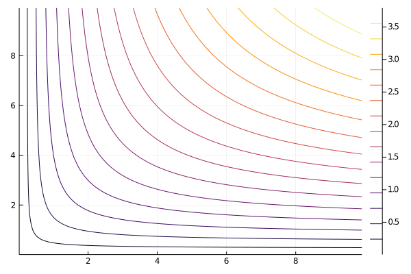
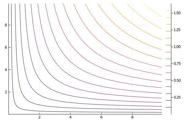
Figure 3: Top: True $(1,10)$-Clayton Lévy copula. Middle: Miss-specified fitted symmetric $(0.355,0.355)$-Clayton Lévy copula. Bottom: crossing of both forementioned $\boldsymbol{\alpha}$-Clayton Lévy copulas, darker lines correspond to the symmetric case as can be seen from the contour levels of the previous plots.

We also fitted a miss-specified symmetric model with fixed $\alpha_{1}=\alpha_{2}=\alpha$ and $\beta_{1}=\beta_{2}=1$, such model coincides with the use of a Clayton Lévy copula when $\alpha=1$. For $T=100$ we obtained fits $\hat{\alpha}=0.355$ and $\hat{\sigma}=0.625$. For illustration purpose we show in Figure 3 the fitted Lévy copulas for the miss-specified and specified model, where we can appreciate the inadequacies of modeling asymmetric observations with a symmetric Lévy copula.

5.2 Danish fire insurance dataset study

In tis section we perform a real data analysis of the Danish fire insurance dataset available in the ”fitdistrplus” R package, see Delignette-Muller and Dutang (2015). The data consist of the losses, in millions of Danish Krone, pertaining to 2167 fire incidents in Copenhagen between 1980 to 1990. We follow Esmaeili and Klüppelberg (2010) and take only into account the building and content losses. Furthermore we focus on losses such that the loss due to the building and due to the contents are both greater than 750000 Danish Kronen or one is greater than 750000 Danish Kronen while the other is zero, so we get 1066 observations. Following their approach, we consider the logarithm of the loss quantities and normalize them by subtracting $\log(0.75)$; thus obtaining the bivariate weights, at each time point, which we model through a bivariate compound Poisson process. In Figures 4 and 5 we show the corresponding bivariate Poisson process. We fit the model in a two-step way by following Esmaeili and Klüppelberg (2013), see also Jiang et al. (2019). In particular, we fit the marginal parameters first and the dependence parameters in the Lévy copula secondly. The marginal distributions, $F_{1}$ and $F_{2}$ are fitted via maximum likelihood and modeled with Gamma distributions, as in comparison with Weibull and LogNormal distributions such choice gave a lower uniform distance between the fitted cumulative distribution function and the empirical; this marginal fits are showed in Figure 6. We fit the $\boldsymbol{\alpha}$-Clayton Lévy copula parameters $\theta=\frac{1}{\sigma}$, $\alpha_{1}$ and $\alpha_{2}$ using maximum likelihood. In Figures 7 and 8 we show the fitted cumulative distributions for the dependent component losses of building and contents, $(w_{1,i}^{\parallel},w_{2,i}^{\parallel})$, and the independent component losses due to building and contents, $w_{1,i}^{\perp}$, $w_{2,i}^{\perp}$, with the respective empirical cumulative distributions for comparison. We observe that the model shows flexibility in fitting the dependent and independent components while the marginal fits as in Figure 6 are kept fixed. We used again the Nelder-Mead algorithm, see previous subsection, and found a maximum loglikelihood value of $-4920.20$. We also found the maximum likelihood estimators for the $\boldsymbol{\alpha}$-Clayton Lévy copula constrained to be symmetric, $\alpha_{1}=\alpha_{2}$ and for the Clayton Lévy copula, $\alpha_{1}=\alpha_{2}=1$, where we got maximum loglikelihood values of, respectively $-4925.62$ and $-4925.75$. It is natural that the unrestricted model can attain a higher likelihood value, which for datasets presenting asymmetry on the underlying Lévy copula must have a significative difference.

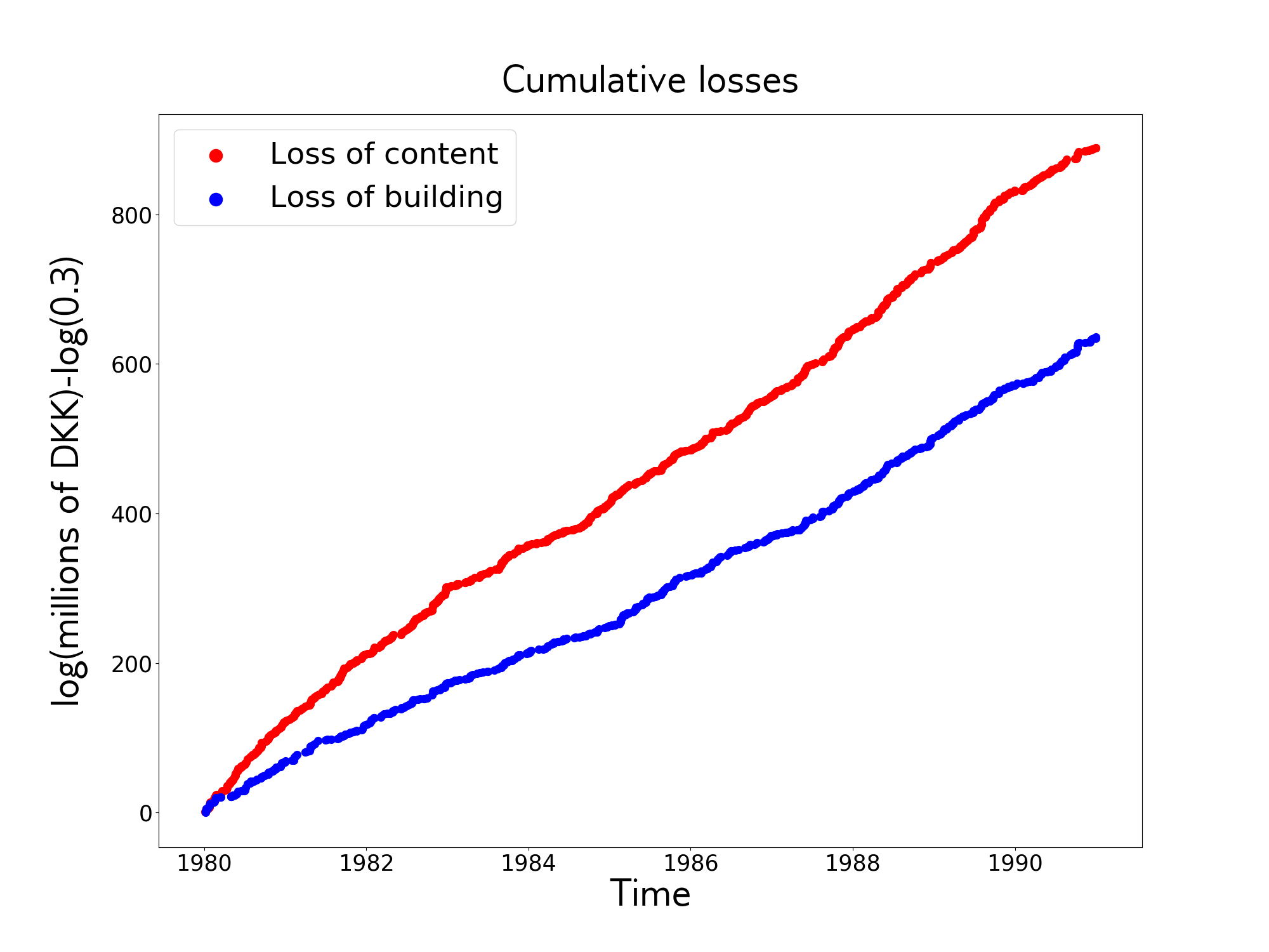
Figure 4: Cumulative logarithmic losses related to loss of content (blue) and loss of building (red) in the Danish fire insurance data as discussed in Section 5.

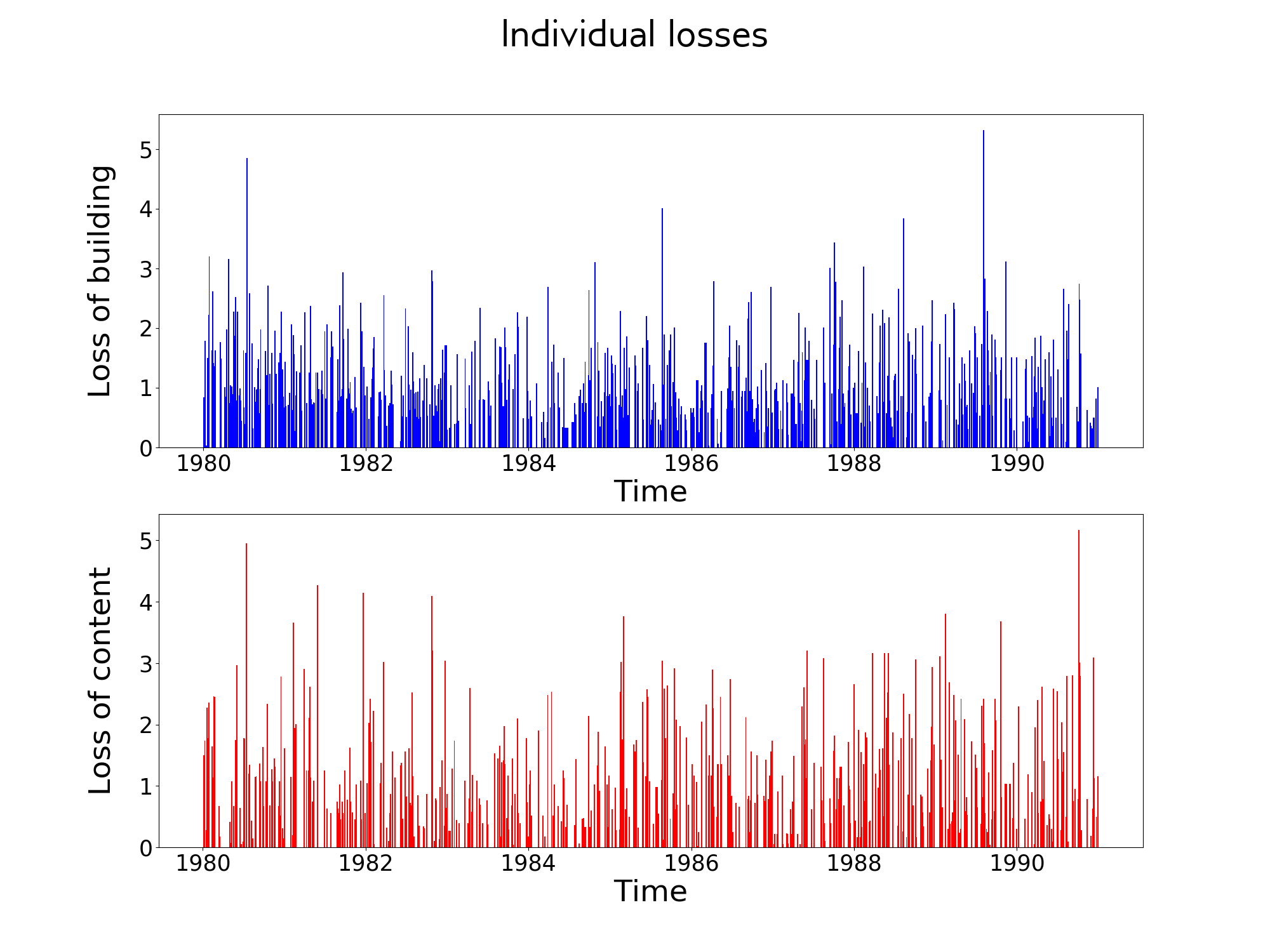
Figure 5: Individual logarithmic losses related to losses due to the building (top) and losse due to content (bottom) in the Danish fire insurance data as discussed in Section 5.

Marginal fits

Figure 6: Marginal fit for the marginal cumulative distribution function (CDF) associated to the losses due to the building (top) and due to content (bottom) in the Danish fire insurance dataset as discussed in Section 5. The black lines correspond to the empirical cumulative distribution function (ECDF) and the red lines corresponds to the maximum likelihood fits with Gamma distributions.

Independent losses fits

Figure 7: Marginal fit for the independent losses, $w_{1,i}^{\perp}$, $w_{2,i}^{\perp}$, cumulative distribution function (CDF) associated to the losses due to the building (top) and due to content (bottom) in the Danish fire insurance dataset as discussed in Section 5. The black lines correspond to the empirical cumulative distribution function (ECDF) and the red lines corresponds to the maximum likelihood fits for the $\boldsymbol{\alpha}$-Clayton Lévy copula.

Dependent losses fits

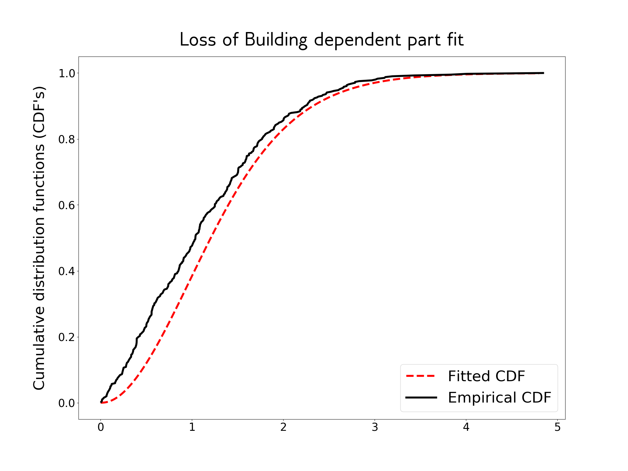
Figure 8: Marginal fit for the dependent losses, $(w_{1,i}^{\parallel},w_{2,i}^{\parallel})$, cumulative distribution function (CDF) associated to the losses due to the building (top) and due to content (bottom) in the Danish fire insurance dataset as discussed in Section 5. The black lines correspond to the empirical cumulative distribution function (ECDF) and the red lines corresponds to the maximum likelihood fits for the $\boldsymbol{\alpha}$-Clayton Lévy copula.

6 Discussion

Diverse families of Lévy copulas have been proposed such as archimedean Lévy copulas, see Proposition 5.6 and 5.7 in Cont and Tankov (2004), vine Lévy copulas, see Grothe and Nicklas (2013) and pareto Lévy copulas, see Eder and Klüppelberg (2012). Pareto and archimedean Lévy copulas are symmetric by construction while vine Lévy copulas can be asymmetric either by using an asymmetric distributional or Lévy copula in their construction. $\boldsymbol{\alpha}$-Clayton Lévy copulas thus help to enrich the examples of asymmetric Lévy copulas in the literature. Extension to arbitrary dimension $d$ is possible by generalizing Theorem 1 into a $d$-variate setting by using a $d$-variate score distribution which has independent Gamma marginals, however the change of variable for obtaining the tail integral, see the proof of Theorem 7, becomes analytically cumbersome as it involves the cumulative distribution function of a Dirichlet distribution. Further choices for the score distribution and directing Lévy measure of a compound vector of subordinators can be considered. An example that we have found to be useful in applications is to use LogNormal score distributions with which the mass of the score distribution can be adequately distributed distributed in $d$-dimensions, see (3). Such choice of score distribution is seen to define a well posed compound vector of subordinators by use of Theorem 5. However such choice seems to usually not be analytically tractable, for example with $\sigma$-stable and gamma directing Lévy measures. The study of the numerical treatment for the Lévy copulas associated to compound vectors of subordinators is left as future work.

Appendix A Proofs

Proof of Theorem 1

By Definition 4, the corresponding Lévy intensity is

$$\rho(\mathrm{d}s_{1},\mathrm{d}s_{2}) =\frac{\sigma K\beta_{1}^{\alpha_{1}}\beta_{2}^{\alpha_{2}}s_{1}^{\alpha_{1}-1}s_{2}^{\alpha_{2}-1}}{\Gamma(\alpha_{1})\Gamma(\alpha_{2})}\int_{0}^{\infty}\left(\frac{1}{z}\right)^{2+\alpha_{1}+\alpha_{2}+\sigma-1}e^{-(\beta_{1}s_{1}+\beta_{2}s_{2})\frac{1}{z}}\mathrm{d}z$$

$$=\frac{\sigma K\beta_{1}^{\alpha_{1}}\beta_{2}^{\alpha_{2}}s_{1}^{\alpha_{1}-1}s_{2}^{\alpha_{2}-1}}{\Gamma(\alpha_{1})\Gamma(\alpha_{2})}\int_{0}^{\infty}u^{\alpha_{1}+\alpha_{2}+\sigma-1}e^{-(\beta_{1}s_{1}+\beta_{2}s_{2})u}\mathrm{d}u$$

$$=\frac{\sigma K\beta_{1}^{\alpha_{1}}\beta_{2}^{\alpha_{2}}\Gamma(\alpha_{1}+\alpha_{2}+\sigma)s_{1}^{\alpha_{1}-1}s_{2}^{\alpha_{2}-1}}{\Gamma(\alpha_{1})\Gamma(\alpha_{2})(\beta_{1}s_{1}+\beta_{2}s_{2})^{\alpha_{1}+\alpha_{2}+\sigma}}$$

And the corresponding marginals are given by

$$\rho_{i}(\mathrm{d}s) =\frac{\sigma K\beta_{i}^{\alpha_{i}}s^{\alpha_{i}-1}}{\Gamma(\alpha_{i})}\int_{0}^{\infty}\left(\frac{1}{z}\right)^{2+\alpha_{i}+\sigma-1}e^{-\beta_{i}s\frac{1}{z}}\mathrm{d}z$$

$$=\frac{\sigma K\beta_{i}^{\alpha_{i}}s^{\alpha_{i}-1}}{\Gamma(\alpha_{i})}\int_{0}^{\infty}u^{\alpha_{i}+\sigma-1}e^{-\beta_{i}su}\mathrm{d}u$$

$$=\frac{\sigma K\beta_{i}^{-\sigma}\Gamma(\alpha_{i}+\sigma)s^{-\sigma-1}}{\Gamma(\alpha_{i})}.$$

The marginal tail integral is

$$U_{i}(y)=\int_{y}^{\infty}\rho_{i}(\mathrm{d}s)=\frac{K\beta_{i}^{-\sigma}\Gamma(\alpha_{i}+\sigma)}{\Gamma(\alpha_{i})}\int_{y}^{\infty}\sigma s^{-\sigma-1}=\frac{K\beta_{i}^{-\sigma}\Gamma(\alpha_{i}+\sigma)y^{-\sigma}}{\Gamma(\alpha_{i})}$$

which has inverse

$$U_{i}^{-1}(y)=\left(\frac{\Gamma(\alpha_{i})y}{K\beta_{i}^{-\sigma}\Gamma(\alpha_{i}+\sigma)}\right)^{-\frac{1}{\sigma}}$$

Proof of Theorem 4

For this proof we will use Proposition 2.1 in Rosinski (2001). Let $H$ be the probability distribution associated to $h$ and $\nu^{\star}$ the directing Lévy intensity. We consider a Poisson random measure

$$M=\sum_{i=1}^{\infty}\delta_{\left(\boldsymbol{Z}_{i},W_{i},X_{i}\right)},$$

where $\{\boldsymbol{Z}_{i}\}_{i=1}^{\infty}\stackrel{{\scriptstyle\text{i.i.d.}}}{{\sim}}H$ and $\{\left(W_{i},X_{i}\right)\}_{i=1}^{\infty}$ are such that

$$\sum_{i=1}^{\infty}\delta_{\left(W_{i},X_{i}\right)},$$

as a Poisson random measure, has intensity $\nu^{\star}$. It follows that $M$ has intensity $\mu=H\times\nu^{\star}$. We define

$$g(\boldsymbol{z},w,x)=(z_{1}w,z_{2}w,\ldots,z_{d}w,x).$$

Due to Proposition 2.1 in Rosinski (2001) it suffices to check that $\nu=\mu\circ g^{-1}$. Let $A_{1},\ldots,A_{d},B\in\mathcal{B}\left(\mathbb{R}^{+}\right)$, then

$$g^{-1}\left((A_{1}\times\ldots\times A_{d})\times B\right)=$$

$$\left\{\left(\frac{a_{1}}{w},\frac{a_{2}}{w},\ldots,\frac{a_{d}}{w},w,x\right)\text{ such that }x\in B,\;a_{1}\in A_{1},\ldots a_{d}\in A_{d},\;w\in\mathbb{R}^{+}\right\}$$

So the pullback measure $\eta=\mu\circ g^{-1}$ is given by

$$\eta\left((A_{1}\times\ldots\times\times A_{d})\times B\right)=\int_{g^{-1}((A_{1}\times\ldots\times\times A_{d})\times B)}\mathrm{d}\mu$$

$$=\int_{A_{1}/z\times A_{2}/z\times\ldots\times A_{d}/z\times(0,\infty)\times B}H(\mathrm{d}s_{1},\ldots,\mathrm{d}s_{d})\nu^{\star}(\mathrm{d}z,\mathrm{d}x)$$

$$=\int_{A_{1}\times A_{2}\times\ldots\times A_{d}\times(0,\infty)\times B}H\left(\frac{\mathrm{d}s_{1}}{z},\ldots,\frac{\mathrm{d}s_{d}}{z}\right)\nu^{\star}(\mathrm{d}z,\mathrm{d}x)$$

So extending the measure we conclude that $\nu=\mu\circ g^{-1}$ so

$$N=\sum_{i=1}^{\infty}\delta_{(Z_{1,i}W_{i},Z_{2,i}W_{i},\ldots,Z_{d,i}W_{i},X_{i})}$$

is almost surely a compound vector of subordinators given by the score distribution $h$ and the directing Lévy measure $\nu^{\star}$ due to Proposition 2.1 in Rosinski (2001).

Proof of Theorem 5

Let $|\boldsymbol{w}|=\sum_{i=1}^{d}w_{i}$ for $\boldsymbol{w}\in(\mathbb{R}^{+})^{d}$. We have that $\|z\boldsymbol{w}\|\leq z|\boldsymbol{w}|$ so

$$\int_{(\mathbb{R}^{+})^{d}\times\mathbb{R}^{+}}\min\left\{1,\|\boldsymbol{s}\|\right\}\nu(\mathrm{d}\boldsymbol{s},\mathrm{d}x)=\int_{(\mathbb{R}^{+})^{d}\times\mathbb{R}^{+}\times\mathbb{R}^{+}}\min\left\{1,\|z\boldsymbol{w}\|\right\}h(\boldsymbol{w})\mathrm{d}\boldsymbol{w}\nu^{\star}(\mathrm{d}z,\mathrm{d}x)$$

$$\leq\int_{(\mathbb{R}^{+})^{d}\times\mathbb{R}^{+}\times\mathbb{R}^{+}}\min\left\{1,z|\boldsymbol{w}|\right\}h(\boldsymbol{w})\mathrm{d}\boldsymbol{w}\nu^{\star}(\mathrm{d}z,\mathrm{d}x)=\mathbb{E}\!\left[\int_{(\mathbb{R}^{+})^{2}}\min\left\{1,z|\boldsymbol{W}|\right\}\nu^{\star}(\mathrm{d}z,\mathrm{d}x)\right]$$

$$=\mathbb{E}\!\left[\int_{\left(0,\frac{1}{|\boldsymbol{W}|}\right)\times\mathbb{R}^{+}}z|\boldsymbol{W}|\nu^{\star}(\mathrm{d}z,\mathrm{d}x)\right]+\mathbb{E}\!\left[\int_{\left[\frac{1}{|\boldsymbol{W}|},\infty\right)\times\mathbb{R}^{+}}\nu^{\star}(\mathrm{d}z,\mathrm{d}x)\right]$$

$$=\mathbb{E}\!\left[\int_{\mathbb{R}^{+}\times\mathbb{R}^{+}}\mathbbm{1}_{\left\{z<\frac{1}{|\boldsymbol{W}|}\right\}}z|\boldsymbol{W}|\nu^{\star}(\mathrm{d}z,\mathrm{d}x)\right]+\mathbb{E}\!\left[\int_{\mathbb{R}^{+}\times\mathbb{R}^{+}}\mathbbm{1}_{\left\{\frac{1}{|\boldsymbol{W}|}\leq z\right\}}\nu^{\star}(\mathrm{d}z,\mathrm{d}x)\right]$$

$$=\int_{(0,1)\times\mathbb{R}^{+}}\mathbb{E}\!\left[\mathbbm{1}_{\left\{|\boldsymbol{W}|<\frac{1}{z}\right\}}|\boldsymbol{W}|\right]z\nu^{\star}(\mathrm{d}z,\mathrm{d}x)+\int_{[1,\infty)\times\mathbb{R}^{+}}\mathbb{E}\!\left[\mathbbm{1}_{\left\{|\boldsymbol{W}|<\frac{1}{z}\right\}}|\boldsymbol{W}|\right]z\nu^{\star}(\mathrm{d}z,\mathrm{d}x)$$

$$\hphantom{=}+\int_{(0,1)\times\mathbb{R}^{+}}\mathbb{E}\!\left[\mathbbm{1}_{\left\{|\boldsymbol{W}|\geq\frac{1}{z}\right\}}\right]\nu^{\star}(\mathrm{d}z,\mathrm{d}x)+\int_{[1,\infty)\times\mathbb{R}^{+}}\mathbb{E}\!\left[\mathbbm{1}_{\left\{|\boldsymbol{W}|\geq\frac{1}{z}\right\}}\right]\nu^{\star}(\mathrm{d}z,\mathrm{d}x)$$

$$\leq\mathbb{E}\!\left[|\boldsymbol{W}|\right]\int_{(0,1)\times\mathbb{R}^{+}}z\nu^{\star}(\mathrm{d}z,\mathrm{d}x)+\int_{[1,\infty)\times\mathbb{R}^{+}}\nu^{\star}(\mathrm{d}z,\mathrm{d}x)$$

$$\hphantom{=}+\mathbb{E}\!\left[|\boldsymbol{W}|\right]\int_{(0,1)\times\mathbb{R}^{+}}z\nu^{\star}(\mathrm{d}z,\mathrm{d}x)+\int_{[1,\infty)\times\mathbb{R}^{+}}\nu^{\star}(\mathrm{d}z,\mathrm{d}x)<\infty.$$

For the first and fourth integral we use the fact that the indicator function is less or equal to one. For the second integral, we note that $\mathbb{E}\!\left[\mathbbm{1}_{\left\{|\boldsymbol{W}|<\frac{1}{z}\right\}}z|\boldsymbol{W}|\right]\leq 1$. For the third integral, we use the Markov’s inequality, $\mathbb{E}\!\left[\mathbbm{1}_{\left\{|\boldsymbol{W}|\geq\frac{1}{z}\right\}}\right]=\mathbb{P}\!\left[|\boldsymbol{W}|\geq\frac{1}{z}\right]\leq z\mathbb{E}\!\left[|\boldsymbol{W}|\right]$. Finiteness of the above expression follows from the fact that $\nu^{\star}$ is a Lévy intensity satisfying (1) and $\mathbb{E}\!\left[|\boldsymbol{W}|\right]<\infty$.

Proof of Theorem 6

We can set the multivariate Lévy intensity for a $d-$variate vector of subordinators $\boldsymbol{Y}=\left(Y_{1},\ldots,Y_{d}\right)$ with $\boldsymbol{\lambda}=\left(\lambda_{1},\ldots,\lambda_{d}\right)$ as

$$\psi_{t}(\boldsymbol{\lambda})=\int_{0}^{t}\int_{0}^{\infty}(1-e^{-\lambda_{1}s_{1}-\ldots-\lambda_{d}s_{d}})\nu(\mathrm{d}s,\mathrm{d}x)=-\log\left(\mathbb{E}\!\left[e^{-\lambda_{1}Y_{1}(t)-\ldots-\lambda_{d}Y_{d}}\right]\right).$$

If we denote $\{\boldsymbol{e}_{i}\}_{i=1}^{d}$ as the canonical basis of $\mathbb{R}^{d}$ and the univariate Laplace exponent of $Y_{i}$ as $\psi_{t}(\lambda\boldsymbol{e}_{i})=-\log\left(\mathbb{E}\!\left[e^{-\lambda Y_{i}(t)}\right]\right)$ in Definition 2; we have that

$$\mathbb{E}\!\left[Y_{i}(t)\right]={\left.\kern-1.2pt-\frac{\partial}{\partial\lambda}\mathbb{E}\!\left[e^{-\lambda Y_{i}(t)}\right]\vphantom{\big{|}}\right|_{\lambda=0}}={\left.\kern-1.2pt-\frac{\partial}{\partial\lambda}e^{-\psi_{t}(\lambda\boldsymbol{e}_{i})}\vphantom{\big{|}}\right|_{\lambda=0}}={\left.\kern-1.2pt-\frac{\partial}{\partial\lambda}e^{-\mathbb{E}\!\left[\,\psi_{t}^{\star}(\lambda W_{i})\right]}\vphantom{\big{|}}\right|_{\lambda=0}}$$

$$={\left.\kern-1.2pte^{-\mathbb{E}\!\left[\,\psi_{t}^{\star}(\lambda W_{i})\right]}\mathbb{E}\!\left[\,(\psi_{t}^{\star})^{\prime}(\lambda W_{i})W_{i}\right]\vphantom{\big{|}}\right|_{\lambda=0}}=(\psi_{t}^{\star})^{\prime}(0)\mathbb{E}\!\left[W_{i}\right]$$

For $0<p<1$ we can use Theorem 1 in Wolfe (1975) to obtain that

$$\mathbb{E}\!\left[\left(Y_{i}(t)\right)^{p}\right]=\frac{p}{\Gamma(1-p)}\int_{0}^{\infty}\frac{1-e^{-\psi_{t}(u\boldsymbol{e}_{i})}}{u^{p+1}}\mathrm{d}u=\frac{p}{\Gamma(1-p)}\int_{0}^{\infty}\frac{1-e^{-\mathbb{E}\!\left[\psi^{\star}_{t}(uW_{i})\right]}}{u^{p+1}}\mathrm{d}u$$

We observe that

$$\mathbb{E}\!\left[Y_{i}^{2}(t)\right]={\left.\kern-1.2pt\frac{\partial^{2}}{\partial\lambda\partial\lambda}\mathbb{E}\!\left[e^{-\lambda Y_{i}(t)}\right]\vphantom{\big{|}}\right|_{\lambda=0}}={\left.\kern-1.2pt\frac{\partial^{2}}{\partial\lambda\partial\lambda}e^{-\psi_{t}(\lambda\boldsymbol{e}_{i})}\vphantom{\big{|}}\right|_{\lambda=0}}={\left.\kern-1.2pt\frac{\partial^{2}}{\partial\lambda\partial\lambda}e^{-\mathbb{E}\!\left[\psi_{t}^{\star}(\lambda W_{i})\right]}\vphantom{\big{|}}\right|_{\lambda=0}}$$

$$={\left.\kern-1.2pt\frac{\partial}{\partial\lambda}e^{-\mathbb{E}\!\left[\psi_{t}^{\star}(\lambda W_{i})\right]}(-1)\mathbb{E}\!\left[(\psi_{t}^{\star})^{\prime}(\lambda W_{i})W_{i}\right]\vphantom{\big{|}}\right|_{\lambda=0}}$$

$$={\left.\kern-1.2pt\left(e^{-\mathbb{E}\!\left[\psi_{t}^{\star}(\lambda W_{i})\right]}(\mathbb{E}\!\left[(\psi_{t}^{\star})^{\prime}(\lambda W_{i})W_{i}\right])^{2}-e^{-\mathbb{E}\!\left[\psi_{t}^{\star}(\lambda W_{i})\right]}\mathbb{E}\!\left[(\psi_{t}^{\star})^{\prime\prime}(\lambda W_{i})W_{i}^{2}\right]\right)\vphantom{\big{|}}\right|_{\lambda=0}}$$

$$=\left((\psi_{t}^{\star})^{\prime}(0)\right)^{2}\mathbb{E}\!\left[W_{i}\right]^{2}-(\psi_{t}^{\star})^{\prime\prime}(0)\mathbb{E}\!\left[W_{i}^{2}\right].$$

It follows that

$$\text{Var}\!\left(Y_{i}(t)\right) =\mathbb{E}\!\left[Y_{i}^{2}(t)\right]-\mathbb{E}\!\left[Y_{i}(t)\right]^{2}=\left((\psi_{t}^{\star})^{\prime}(0)\right)^{2}\mathbb{E}\!\left[W_{i}\right]^{2}-(\psi_{t}^{\star})^{\prime\prime}(0)\mathbb{E}\!\left[W_{i}^{2}\right]-\left((\psi_{t}^{\star})^{\prime}(0)\right)^{2}\mathbb{E}\!\left[W_{i}\right]^{2}$$

$$=-(\psi_{t}^{\star})^{\prime\prime}(0)\mathbb{E}\!\left[W_{i}^{2}\right]$$

For $i,j\in\left\{1,\ldots,n\right\}$, $i\neq j$ observe that

$$\mathbb{E}\!\left[Y_{i}(t)Y_{j}(t)\right]={\left.\kern-1.2pt\frac{\partial^{2}}{\partial\lambda_{j}\partial\lambda_{i}}\mathbb{E}\!\left[e^{-\lambda_{i}Y_{i}(t)-\lambda_{j}Y_{j}(t)}\right]\vphantom{\big{|}}\right|_{\lambda_{i}=\lambda_{j}=0}}={\left.\kern-1.2pt\frac{\partial^{2}}{\partial\lambda_{j}\partial\lambda_{i}}e^{-\psi_{t}(\lambda_{i}\boldsymbol{e}_{i}+\lambda_{j}\boldsymbol{e}_{j})}\vphantom{\big{|}}\right|_{\lambda_{i}=\lambda_{j}=0}}$$

$$={\left.\kern-1.2pt\frac{\partial^{2}}{\partial\lambda_{j}\partial\lambda_{i}}e^{-\mathbb{E}\!\left[\psi_{t}^{\star}(\lambda_{i}W_{i}+\lambda_{j}W_{j})\right]}\vphantom{\big{|}}\right|_{\lambda_{i}=\lambda_{j}=0}}={\left.\kern-1.2pt\frac{\partial}{\partial\lambda_{j}}e^{-\mathbb{E}\!\left[\psi_{t}^{\star}(\lambda_{i}W_{i}+\lambda_{j}W_{j})\right]}(-1)\mathbb{E}\!\left[(\psi_{t}^{\star})^{\prime}(\lambda_{i}W_{i}+\lambda_{j}W_{j})W_{i}\right]\vphantom{\big{|}}\right|_{\lambda_{i}=\lambda_{j}=0}}$$

$$=\left(e^{-\mathbb{E}\!\left[\psi_{t}^{\star}(\lambda_{i}W_{i}+\lambda_{j}W_{j})\right]}\mathbb{E}\!\left[(\psi_{t}^{\star})^{\prime}(\lambda_{i}W_{i}+\lambda_{j}W_{j})W_{j}\right]\mathbb{E}\!\left[(\psi_{t}^{\star})^{\prime}(\lambda_{i}W_{i}+\lambda_{j}W_{j})W_{i}\right]\right.$$

$$\hphantom{=}{\left.\kern-1.2pt\left.-e^{-\mathbb{E}\!\left[\psi_{t}^{\star}(\lambda_{i}W_{i}+\lambda_{j}W_{j})\right]}\mathbb{E}\!\left[(\psi_{t}^{\star})^{\prime\prime}(\lambda_{i}W_{i}+\lambda_{j}W_{j})W_{i}W_{j}\right]\right)\vphantom{\big{|}}\right|_{\lambda_{i}=\lambda_{j}=0}}$$

$$=\left((\psi_{t}^{\star})^{\prime}(0)\right)^{2}\mathbb{E}\!\left[W_{j}\right]\mathbb{E}\!\left[W_{i}\right]-\mathbb{E}\!\left[(\psi_{t}^{\star})^{\prime\prime}(0)W_{i}W_{j}\right]$$

We get that

$$Cov\!\left(Y_{i}(t),Y_{j}(t)\right) =\mathbb{E}\!\left[Y_{i}(t)Y_{j}(t)\right]-\mathbb{E}\!\left[Y_{i}(t)\right]\mathbb{E}\!\left[Y_{j}(t)\right]$$

$$=\left((\psi_{t}^{\star})^{\prime}(0)\right)^{2}\mathbb{E}\!\left[W_{j}\right]\mathbb{E}\!\left[W_{i}\right]-\mathbb{E}\!\left[(\psi_{t}^{\star})^{\prime\prime}(0)W_{i}W_{j}\right]-\left((\psi_{t}^{\star})^{\prime}(0)\right)^{2}\mathbb{E}\!\left[W_{i}\right]\mathbb{E}\!\left[W_{j}\right]$$

$$=-(\psi_{t}^{\star})^{\prime\prime}(0)\mathbb{E}\!\left[W_{i}W_{j}\right]$$

It follows that

$$Cor\!\left(Y_{i}(t),Y_{j}(t)\right) =\frac{Cov\!\left(Y_{i}(t),Y_{j}(t)\right)}{\sqrt{\text{Var}\!\left(Y_{i}(t)\right)}\sqrt{\text{Var}\!\left(Y_{j}(t)\right)}}=\frac{-(\psi_{t}^{\star})^{\prime\prime}(0)\mathbb{E}\!\left[W_{i}W_{j}\right]}{\sqrt{\left((\psi_{t}^{\star})^{\prime\prime}(0)\right)^{2}\mathbb{E}\!\left[W_{i}^{2}\right]\mathbb{E}\!\left[W_{j}^{2}\right]}}$$

$$=\frac{\mathbb{E}\!\left[W_{i}W_{j}\right]}{\sqrt{\mathbb{E}\!\left[W_{i}^{2}\right]\mathbb{E}\!\left[W_{j}^{2}\right]}}$$

Proof of Theorem 7

Proof of a)
The proof strategy is to use (2) in order to obtain the corresponding Lévy copula. As first step, we obtain the bivariate tail integral associated to $\rho_{\sigma,K,\boldsymbol{\alpha},\boldsymbol{\beta}}$ as in the hypothesis; we denote this tail integral by $U$.

$$U(y_{1},y_{2}) =\int_{y_{1}}^{\infty}\int_{y_{2}}^{\infty}\frac{\sigma K\beta_{1}^{\alpha_{1}}\beta_{2}^{\alpha_{2}}\Gamma(\alpha_{1}+\alpha_{2}+\sigma)s_{1}^{\alpha_{1}-1}s_{2}^{\alpha_{2}-1}(\beta_{1}s_{1}+\beta_{2}s_{2})^{-\alpha_{1}-\alpha_{2}-\sigma}}{\Gamma(\alpha_{1})\Gamma(\alpha_{2})}\mathrm{d}s_{1}\mathrm{d}s_{2}$$

$$=\int_{\beta_{1}y_{1}}^{\infty}\int_{\beta_{2}y_{2}}^{\infty}\frac{\sigma K\Gamma(\alpha_{1}+\alpha_{2}+\sigma)s_{1}^{\alpha_{1}-1}s_{2}^{\alpha_{2}-1}(s_{1}+s_{2})^{-\alpha_{1}-\alpha_{2}-\sigma}}{\Gamma(\alpha_{1})\Gamma(\alpha_{2})}\mathrm{d}s_{1}\mathrm{d}s_{2}$$

We consider the change of variable

$$\boldsymbol{h}(s_{1},s_{2}) =(s_{1}+s_{2},s_{1}/(s_{1}+s_{2}))=(\rho,z_{1})$$

$$\mathrm{d}\rho\mathrm{d}z_{1} =\left|\det(\frac{\mathrm{d}\boldsymbol{h}}{\mathrm{d}\boldsymbol{s}})\right|\mathrm{d}s_{1}\mathrm{d}s_{2}=(s_{1}+s_{2})^{-1}\mathrm{d}s_{1}\mathrm{d}s_{2}$$

so

$$U(y_{1},y_{2})=\frac{\sigma K\Gamma(\alpha_{1}+\alpha_{2}+\sigma)}{\Gamma(\alpha_{1})\Gamma(\alpha_{2})}$$

$$\times\int_{h\left(\left\{s_{1},s_{2}\,:\,\beta_{1}y_{1}\leq s_{1}\,,\,\beta_{2}y_{2}\leq s_{2}\right\}\right)}z_{1}^{\alpha_{1}-1}(1-z_{1})^{\alpha_{2}-1}\rho^{-\sigma-1}\mathrm{d}\rho\mathrm{d}z_{1}.$$

Throughout the proof, we denote with $c_{\sigma,\boldsymbol{\alpha}}$ the following quantity

$$c_{\sigma,\boldsymbol{\alpha}}=\frac{K\Gamma(\alpha_{1}+\alpha_{2}+\sigma)}{\Gamma(\alpha_{1})\Gamma(\alpha_{2})}$$

For the integration region, we consider the curves

$$\hat{\omega}(\hat{t}) =h(\beta_{1}y_{1},\beta_{2}y_{2}+\hat{t})=(\beta_{1}y_{1}+\beta_{2}y_{2}+\hat{t},\beta_{1}y_{1}/(\beta_{1}y_{1}+\beta_{2}y_{2}+\hat{t}))$$

$$\hat{\gamma}(\hat{t}) =h(\beta_{1}y_{1}+\hat{t},y_{2})=(\beta_{1}y_{1}+\beta_{2}y_{2}+\hat{t},(\beta_{1}y_{1}+\hat{t})/(\beta_{1}y_{1}+\beta_{2}y_{2}+\hat{t}))$$

with $\hat{t}\geq 0$; so for $t_{1}=\beta_{1}y_{1}/(\beta_{1}y_{1}+\beta_{2}y_{2}+\hat{t})$ and $t_{2}=(\beta_{1}y_{1}+\hat{t})/(\beta_{1}y_{1}+\beta_{2}y_{2}+\hat{t})$ we can get the reparametrized curves $\omega(t_{1})=(\beta_{1}y_{1}/t_{1},t_{1})$ and $\gamma(t_{2})=(\beta_{2}y_{2}/(1-t_{2}),t_{2})$ to delimit the integration area, hence using Fubini theorem

$$U(y_{1},y_{2}) =c_{\sigma,\boldsymbol{\alpha}}\left(\int_{0}^{\frac{\beta_{1}y_{1}}{\beta_{1}y_{1}+\beta_{2}y_{2}}}\int_{\beta_{1}y_{1}/z_{1}}^{\infty}z_{1}^{\alpha_{1}-1}(1-z_{1})^{\alpha_{2}-1}\sigma\rho^{-\sigma-1}\mathrm{d}\rho\mathrm{d}z_{1}\right.$$

$$\hphantom{=}\left.+\int_{\frac{\beta_{1}y_{1}}{\beta_{1}y_{1}+\beta_{2}y_{2}}}^{1}\int_{\beta_{2}y_{2}/(1-z_{1})}^{\infty}z_{1}^{\alpha_{1}-1}(1-z_{1})^{\alpha_{2}-1}\sigma\rho^{-\sigma-1}\mathrm{d}\rho\mathrm{d}z_{1}\right)$$

$$=c_{\sigma,\boldsymbol{\alpha}}\left(\int_{0}^{\frac{\beta_{1}y_{1}}{\beta_{1}y_{1}+\beta_{2}y_{2}}}z_{1}^{\alpha_{1}+\sigma-1}(1-z_{1})^{\alpha_{2}-1}(\beta_{1}y_{1})^{-\sigma}\mathrm{d}z_{1}\right.$$

$$\hphantom{=}\left.+\int_{\frac{\beta_{1}y_{1}}{\beta_{1}y_{1}+\beta_{2}y_{2}}}^{1}z_{1}^{\alpha_{1}-1}(1-z_{1})^{\alpha_{2}+\sigma-1}(\beta_{2}y_{2})^{-\sigma}\mathrm{d}z_{1}\right)$$

$$=c_{\sigma,\boldsymbol{\alpha}}\left(\int_{0}^{\frac{\beta_{1}y_{1}}{\beta_{1}y_{1}+\beta_{2}y_{2}}}z_{1}^{\alpha_{1}+\sigma-1}(1-z_{1})^{\alpha_{2}-1}(\beta_{1}y_{1})^{-\sigma}\mathrm{d}z_{1}\right.$$

$$\hphantom{=}\left.+\int_{0}^{\frac{\beta_{2}y_{2}}{\beta_{1}y_{1}+\beta_{2}y_{2}}}z_{1}^{\alpha_{2}+\sigma-1}(1-z_{1})^{\alpha_{1}-1}(\beta_{2}y_{2})^{-\sigma}\mathrm{d}z_{1}\right)$$

The above expression can be evaluated in terms of cumulative distribution functions of a Beta$(\alpha,\beta)$ random variable which we write as the regularized incomplete beta function $I(x,\alpha,\beta)$. Let $B$ be the beta function $B(a,b)=\Gamma(a)\Gamma(b)/\Gamma(a+b)$, thus

$$U(y_{1},y_{2})=c_{\sigma,\boldsymbol{\alpha}}\left((\beta_{1}y_{1})^{-\sigma}B(\alpha_{1}+\sigma,\alpha_{2})I\left(\frac{\beta_{1}y_{1}}{\beta_{1}y_{1}+\beta_{2}y_{2}},\alpha_{1}+\sigma,\alpha_{2}\right)\right.$$

$$\left.\hphantom{U(y_{1},y_{2})=}+(\beta_{2}y_{2})^{-\sigma}B(\alpha_{1},\alpha_{2}+\sigma)I\left(\frac{\beta_{2}y_{2}}{\beta_{1}y_{1}+\beta_{2}y_{2}},\alpha_{2}+\sigma,\alpha_{1}\right)\right)$$

$$=\frac{K\Gamma(\alpha_{1}+\sigma)(\beta_{1}y_{1})^{-\sigma}}{\Gamma(\alpha_{1})}I\left(\frac{\beta_{1}y_{1}}{\beta_{1}y_{1}+\beta_{2}y_{2}},\alpha_{1}+\sigma,\alpha_{2}\right)$$

$$+\frac{K\Gamma(\alpha_{2}+\sigma)(\beta_{2}y_{2})^{-\sigma}}{\Gamma(\alpha_{2})}I\left(\frac{\beta_{2}y_{2}}{\beta_{1}y_{1}+\beta_{2}y_{2}},\alpha_{2}+\sigma,\alpha_{1}\right)$$

To get the copula we evaluate the above tail integral in

$$\left(U_{1}^{-1}(y_{1}),U^{-1}(y_{2})\right)=\left(\left(\frac{\Gamma(\alpha_{1})y_{1}}{K\beta_{1}^{-\sigma}\Gamma(\alpha_{1}+\sigma)}\right)^{-\frac{1}{\sigma}},\left(\frac{\Gamma(\alpha_{2})y_{2}}{K\beta_{2}^{-\sigma}\Gamma(\alpha_{2}+\sigma)}\right)^{-\frac{1}{\sigma}}\right).$$

So

$$\mathcal{C}(s_{1},s_{2}) =s_{1}\,I\left(\frac{\left(\frac{\Gamma(\alpha_{1}+\sigma)}{\Gamma(\alpha_{1})s_{1}}\right)^{\frac{1}{\sigma}}}{\left(\frac{\Gamma(\alpha_{1}+\sigma)}{\Gamma(\alpha_{1})s_{1}}\right)^{\frac{1}{\sigma}}+\left(\frac{\Gamma(\alpha_{2}+\sigma)}{\Gamma(\alpha_{2})s_{2}}\right)^{\frac{1}{\sigma}}},\alpha_{1}+\sigma,\alpha_{2}\right)$$

$$\hphantom{=}+s_{2}\,I\left(\frac{\left(\frac{\Gamma(\alpha_{2}+\sigma)}{\Gamma(\alpha_{2})s_{2}}\right)^{\frac{1}{\sigma}}}{\left(\frac{\Gamma(\alpha_{1}+\sigma)}{\Gamma(\alpha_{1})s_{1}}\right)^{\frac{1}{\sigma}}+\left(\frac{\Gamma(\alpha_{2}+\sigma)}{\Gamma(\alpha_{2})s_{2}}\right)^{\frac{1}{\sigma}}},\alpha_{2}+\sigma,\alpha_{1}\right)$$

Proof of b)
We perform a constructive proof by using Theorem 6.3 in Cont and Tankov (2004) to show that for $\sigma>1$ a vector of subordinators which has $\mathcal{C}_{\sigma,\boldsymbol{\alpha}}$ as its associated Lévy copula can be given. So $\mathcal{C}_{\sigma,\boldsymbol{\alpha}}$ will be a Lévy copula also for $\sigma>1$. Using Theorem 6.3 in Cont and Tankov (2004), we need to show that $F_{S_{1}|S_{2}=s_{2}}(s_{1})=\frac{\partial}{\partial s_{2}}\mathcal{C}_{\sigma,\boldsymbol{\alpha}}(s_{1},s_{2})$ and $F_{S_{2}|S_{1}=s_{1}}(s_{2})=\frac{\partial}{\partial s_{1}}\mathcal{C}_{\sigma,\boldsymbol{\alpha}}(s_{1},s_{2})$ are cumulative distribution functions. We observe that

$$\frac{\partial}{\partial s_{1}}\mathcal{C}_{\sigma,\boldsymbol{\alpha}}(s_{1},s_{2})=\frac{\Gamma(\alpha_{1}+\alpha_{2}+\sigma)}{\Gamma(\alpha_{1}+\sigma)\Gamma(\alpha_{2})}\int_{0}^{\frac{\left(\frac{\Gamma(\alpha_{1}+\sigma)}{\Gamma(\alpha_{1})s_{1}}\right)^{\frac{1}{\sigma}}}{\left(\frac{\Gamma(\alpha_{1}+\sigma)}{\Gamma(\alpha_{1})s_{1}}\right)^{\frac{1}{\sigma}}+\left(\frac{\Gamma(\alpha_{2}+\sigma)}{\Gamma(\alpha_{2})s_{2}}\right)^{\frac{1}{\sigma}}}}z^{\alpha_{1}+\sigma-1}(1-z)^{\alpha_{2}-1}\mathrm{d}z$$

$$-\frac{\Gamma(\alpha_{1}+\alpha_{2}+\sigma)}{\sigma\Gamma(\alpha_{1}+\sigma)\Gamma(\alpha_{2})}\frac{\left(\frac{\Gamma(\alpha_{1}+\sigma)}{\Gamma(\alpha_{1})s_{1}}\right)^{\frac{\alpha_{1}+\sigma}{\sigma}}\left(\frac{\Gamma(\alpha_{2}+\sigma)}{\Gamma(\alpha_{2})s_{2}}\right)^{\frac{\alpha_{2}}{\sigma}}}{\left(\left(\frac{\Gamma(\alpha_{1}+\sigma)}{\Gamma(\alpha_{1})s_{1}}\right)^{\frac{1}{\sigma}}+\left(\frac{\Gamma(\alpha_{2}+\sigma)}{\Gamma(\alpha_{2})s_{2}}\right)^{\frac{1}{\sigma}}\right)^{\alpha_{1}+\alpha_{2}+\sigma}}$$

$$+\frac{\Gamma(\alpha_{1}+\alpha_{2}+\sigma)s_{2}}{\sigma\Gamma(\alpha_{2}+\sigma)\Gamma(\alpha_{1})s_{1}}\frac{\left(\frac{\Gamma(\alpha_{1}+\sigma)}{\Gamma(\alpha_{1})s_{1}}\right)^{\frac{\alpha_{1}}{\sigma}}\left(\frac{\Gamma(\alpha_{2}+\sigma)}{\Gamma(\alpha_{2})s_{2}}\right)^{\frac{\alpha_{2}+\sigma}{\sigma}}}{\left(\left(\frac{\Gamma(\alpha_{1}+\sigma)}{\Gamma(\alpha_{1})s_{1}}\right)^{\frac{1}{\sigma}}+\left(\frac{\Gamma(\alpha_{2}+\sigma)}{\Gamma(\alpha_{2})s_{2}}\right)^{\frac{1}{\sigma}}\right)^{\alpha_{1}+\alpha_{2}+\sigma}}$$

$$=\frac{\Gamma(\alpha_{1}+\alpha_{2}+\sigma)}{\Gamma(\alpha_{1}+\sigma)\Gamma(\alpha_{2})}\int_{0}^{\frac{\left(\frac{\Gamma(\alpha_{1}+\sigma)}{\Gamma(\alpha_{1})s_{1}}\right)^{\frac{1}{\sigma}}}{\left(\frac{\Gamma(\alpha_{1}+\sigma)}{\Gamma(\alpha_{1})s_{1}}\right)^{\frac{1}{\sigma}}+\left(\frac{\Gamma(\alpha_{2}+\sigma)}{\Gamma(\alpha_{2})s_{2}}\right)^{\frac{1}{\sigma}}}}z^{\alpha_{1}+\sigma-1}(1-z)^{\alpha_{2}-1}\mathrm{d}z$$

$$-\frac{\Gamma(\alpha_{1}+\alpha_{2}+\sigma)}{\sigma\Gamma(\alpha_{1})\Gamma(\alpha_{2})s_{1}}\frac{\left(\frac{\Gamma(\alpha_{1}+\sigma)}{\Gamma(\alpha_{1})s_{1}}\right)^{\frac{\alpha_{1}}{\sigma}}\left(\frac{\Gamma(\alpha_{2}+\sigma)}{\Gamma(\alpha_{2})s_{2}}\right)^{\frac{\alpha_{2}}{\sigma}}}{\left(\left(\frac{\Gamma(\alpha_{1}+\sigma)}{\Gamma(\alpha_{1})s_{1}}\right)^{\frac{1}{\sigma}}+\left(\frac{\Gamma(\alpha_{2}+\sigma)}{\Gamma(\alpha_{2})s_{2}}\right)^{\frac{1}{\sigma}}\right)^{\alpha_{1}+\alpha_{2}+\sigma}}$$

$$+\frac{\Gamma(\alpha_{1}+\alpha_{2}+\sigma)}{\sigma\Gamma(\alpha_{1})\Gamma(\alpha_{2})s_{1}}\frac{\left(\frac{\Gamma(\alpha_{1}+\sigma)}{\Gamma(\alpha_{1})s_{1}}\right)^{\frac{\alpha_{1}}{\sigma}}\left(\frac{\Gamma(\alpha_{2}+\sigma)}{\Gamma(\alpha_{2})s_{2}}\right)^{\frac{\alpha_{2}}{\sigma}}}{\left(\left(\frac{\Gamma(\alpha_{1}+\sigma)}{\Gamma(\alpha_{1})s_{1}}\right)^{\frac{1}{\sigma}}+\left(\frac{\Gamma(\alpha_{2}+\sigma)}{\Gamma(\alpha_{2})s_{2}}\right)^{\frac{1}{\sigma}}\right)^{\alpha_{1}+\alpha_{2}+\sigma}}$$

$$=\frac{\Gamma(\alpha_{1}+\alpha_{2}+\sigma)}{\Gamma(\alpha_{1}+\sigma)\Gamma(\alpha_{2})}\int_{0}^{\frac{\left(\frac{\Gamma(\alpha_{1}+\sigma)}{\Gamma(\alpha_{1})s_{1}}\right)^{\frac{1}{\sigma}}}{\left(\frac{\Gamma(\alpha_{1}+\sigma)}{\Gamma(\alpha_{1})s_{1}}\right)^{\frac{1}{\sigma}}+\left(\frac{\Gamma(\alpha_{2}+\sigma)}{\Gamma(\alpha_{2})s_{2}}\right)^{\frac{1}{\sigma}}}}z^{\alpha_{1}+\sigma-1}(1-z)^{\alpha_{2}-1}\mathrm{d}z$$

and similarly

$$\frac{\partial}{\partial s_{2}}\mathcal{C}_{\sigma,\boldsymbol{\alpha}}(s_{1},s_{2})=\frac{\Gamma(\alpha_{1}+\alpha_{2}+\sigma)}{\Gamma(\alpha_{2}+\sigma)\Gamma(\alpha_{1})}\int_{0}^{\frac{\left(\frac{\Gamma(\alpha_{2}+\sigma)}{\Gamma(\alpha_{2})s_{2}}\right)^{\frac{1}{\sigma}}}{\left(\frac{\Gamma(\alpha_{1}+\sigma)}{\Gamma(\alpha_{1})s_{1}}\right)^{\frac{1}{\sigma}}+\left(\frac{\Gamma(\alpha_{2}+\sigma)}{\Gamma(\alpha_{2})s_{2}}\right)^{\frac{1}{\sigma}}}}z^{\alpha_{2}+\sigma-1}(1-z)^{\alpha_{1}-1}\mathrm{d}z$$

Either by differentiating the above expressions or by using Theorem 2 we can obtain that

$$\frac{\partial^{2}}{\partial s_{2}\partial s_{1}}\mathcal{C}_{\sigma,\boldsymbol{\alpha}}(s_{1},s_{2})=\frac{\Gamma(\alpha_{1}+\alpha_{2}+\sigma)}{\sigma\Gamma(\alpha_{1})\Gamma(\alpha_{2})s_{1}s_{2}}\frac{\left(\frac{\Gamma(\alpha_{1}+\sigma)}{\Gamma(\alpha_{1})s_{1}}\right)^{\frac{\alpha_{1}}{\sigma}}\left(\frac{\Gamma(\alpha_{2}+\sigma)}{\Gamma(\alpha_{2})s_{2}}\right)^{\frac{\alpha_{2}}{\sigma}}}{\left(\left(\frac{\Gamma(\alpha_{1}+\sigma)}{\Gamma(\alpha_{1})s_{1}}\right)^{\frac{1}{\sigma}}+\left(\frac{\Gamma(\alpha_{2}+\sigma)}{\Gamma(\alpha_{2})s_{2}}\right)^{\frac{1}{\sigma}}\right)^{\alpha_{1}+\alpha_{2}+\sigma}}$$

So for any $\sigma>0$ $F_{S_{1}|S_{2}=s_{2}}(s_{1})$ and $F_{S_{2}|S_{1}=s_{1}}(s_{2})$ are monotone functions. It suffices to check that

$$\lim_{s_{2}\to 0}F_{S_{2}|S_{1}=s_{1}}(s_{2}) =\lim_{s_{2}\to 0}\frac{\partial}{\partial s_{1}}\mathcal{C}_{\sigma,\boldsymbol{\alpha}}(s_{1},s_{2})=0$$

and

$$\lim_{s_{2}\to\infty}F_{S_{2}|S_{1}=s_{1}}(s_{2}) =\lim_{s_{2}\to\infty}\frac{\partial}{\partial s_{1}}\mathcal{C}_{\sigma,\boldsymbol{\alpha}}(s_{1},s_{2})=1,$$

having the case for $F_{S_{1}|S_{2}=s_{2}}(s_{1})$ being analogous. For the first limit we use the monotonous convergence theorem to obtain that

$$\lim_{s_{2}\to 0}\frac{\partial}{\partial s_{1}}\mathcal{C}_{\sigma,\boldsymbol{\alpha}}(s_{1},s_{2}) =\lim_{s_{2}\to 0}\frac{\Gamma(\alpha_{1}+\alpha_{2}+\sigma)}{\Gamma(\alpha_{1}+\sigma)\Gamma(\alpha_{2})}\int_{0}^{\frac{\left(\frac{\Gamma(\alpha_{1}+\sigma)}{\Gamma(\alpha_{1})s_{1}}\right)^{\frac{1}{\sigma}}}{\left(\frac{\Gamma(\alpha_{1}+\sigma)}{\Gamma(\alpha_{1})s_{1}}\right)^{\frac{1}{\sigma}}+\left(\frac{\Gamma(\alpha_{2}+\sigma)}{\Gamma(\alpha_{2})s_{2}}\right)^{\frac{1}{\sigma}}}}z^{\alpha_{1}+\sigma-1}(1-z)^{\alpha_{2}-1}\mathrm{d}z$$

$$=\frac{\Gamma(\alpha_{1}+\alpha_{2}+\sigma)}{\Gamma(\alpha_{1}+\sigma)\Gamma(\alpha_{2})}\int_{0}^{0}z^{\alpha_{1}+\sigma-1}(1-z)^{\alpha_{2}-1}\mathrm{d}z=0$$

So

$$\lim_{s_{2}\to 0}F_{S_{2}|S_{1}=s_{1}}(s_{2})=0.$$

Using the monotonous convergence theorem again we also obtain

$$\lim_{s_{2}\to\infty}\frac{\partial}{\partial s_{1}}\mathcal{C}_{\sigma,\boldsymbol{\alpha}}(s_{1},s_{2}) =\lim_{s_{2}\to\infty}\frac{\Gamma(\alpha_{1}+\alpha_{2}+\sigma)}{\Gamma(\alpha_{1}+\sigma)\Gamma(\alpha_{2})}\int_{0}^{\frac{\left(\frac{\Gamma(\alpha_{1}+\sigma)}{\Gamma(\alpha_{1})s_{1}}\right)^{\frac{1}{\sigma}}}{\left(\frac{\Gamma(\alpha_{1}+\sigma)}{\Gamma(\alpha_{1})s_{1}}\right)^{\frac{1}{\sigma}}+\left(\frac{\Gamma(\alpha_{2}+\sigma)}{\Gamma(\alpha_{2})s_{2}}\right)^{\frac{1}{\sigma}}}}z^{\alpha_{1}+\sigma-1}(1-z)^{\alpha_{2}-1}\mathrm{d}z$$

$$=\frac{\Gamma(\alpha_{1}+\alpha_{2}+\sigma)}{\Gamma(\alpha_{1}+\sigma)\Gamma(\alpha_{2})}\int_{0}^{1}z^{\alpha_{1}+\sigma-1}(1-z)^{\alpha_{2}-1}\mathrm{d}z=1$$

So

$$\lim_{s_{2}\to\infty}F_{S_{2}|S_{1}=s_{1}}(s_{2})=1$$

As these limits do not depend on what values $\sigma$ takes in $(0,\infty)$ we conclude by using Theorem 6.3 in Cont and Tankov (2004) that we can construct a subordinator with the desired Lévy copula for any $\sigma\in(0,\infty)$.

Proof of Theorem 8

We start with the proof for $\sigma\to 0$, i.e. $\theta=\frac{1}{\sigma}\to\infty$. Observe that

$$\lim_{\sigma\to 0}\frac{a^{\frac{1}{\sigma}}}{a^{\frac{1}{\sigma}}+b^{\frac{1}{\sigma}}}=\lim_{\sigma\to 0}\frac{1}{1+\left(\frac{b}{a}\right)^{\frac{1}{\sigma}}}$$

so when $b<a$ the limit is $1$ and when $a<b$ the limit is $0$. On the other hand $\lim_{\sigma\to 0}\frac{\Gamma(a+\sigma)}{\Gamma(a)}=1$ for any $a>0$ so there exists $\delta>0$ such that for $0<\sigma<\delta$ we have that i) $s_{1}<s_{2}\implies\frac{\Gamma(\alpha_{2}+\sigma)}{\Gamma(\alpha_{2})s_{2}}<\frac{\Gamma(\alpha_{1}+\sigma)}{\Gamma(\alpha_{1})s_{1}}$ and ii) $s_{2}<s_{1}\implies\frac{\Gamma(\alpha_{1}+\sigma)}{\Gamma(\alpha_{1})s_{1}}<\frac{\Gamma(\alpha_{2}+\sigma)}{\Gamma(\alpha_{2})s_{2}}$. Without loss of generality we assume that $s_{1}<s_{2}$, the case $s_{2}<s_{1}$ being treated analogously. We consider $0<\sigma<\delta$ and use the bounded convergence theorem to see that

$$\lim_{\sigma\to 0}\mathcal{C}_{\sigma,\boldsymbol{\alpha}}(s_{1},s_{2})=\lim_{\sigma\to 0}\left(s_{1}\frac{\Gamma(\alpha_{1}+\alpha_{2}+\sigma)}{\Gamma(\alpha_{1}+\sigma)\Gamma(\alpha_{2})}\int_{0}^{\frac{\left(\frac{\Gamma(\alpha_{1}+\sigma)}{\Gamma(\alpha_{1})s_{1}}\right)^{\frac{1}{\sigma}}}{\left(\frac{\Gamma(\alpha_{1}+\sigma)}{\Gamma(\alpha_{1})s_{1}}\right)^{\frac{1}{\sigma}}+\left(\frac{\Gamma(\alpha_{2}+\sigma)}{\Gamma(\alpha_{2})s_{2}}\right)^{\frac{1}{\sigma}}}}z^{\alpha_{1}+\sigma-1}(1-z)^{\alpha_{2}-1}\mathrm{d}z\right.$$

$$\left.+s_{2}\frac{\Gamma(\alpha_{1}+\alpha_{2}+\sigma)}{\Gamma(\alpha_{2}+\sigma)\Gamma(\alpha_{1})}\int_{0}^{\frac{\left(\frac{\Gamma(\alpha_{2}+\sigma)}{\Gamma(\alpha_{2})s_{2}}\right)^{\frac{1}{\sigma}}}{\left(\frac{\Gamma(\alpha_{1}+\sigma)}{\Gamma(\alpha_{1})s_{1}}\right)^{\frac{1}{\sigma}}+\left(\frac{\Gamma(\alpha_{2}+\sigma)}{\Gamma(\alpha_{2})s_{2}}\right)^{\frac{1}{\sigma}}}}z^{\alpha_{2}+\sigma-1}(1-z)^{\alpha_{1}-1}\mathrm{d}z\right)$$

$$= s_{1}\frac{\Gamma(\alpha_{1}+\alpha_{2}+\sigma)}{\Gamma(\alpha_{1}+\sigma)\Gamma(\alpha_{2})}\int_{0}^{1}z^{\alpha_{1}+\sigma-1}(1-z)^{\alpha_{2}-1}\mathrm{d}z+s_{2}\frac{\Gamma(\alpha_{1}+\alpha_{2}+\sigma)}{\Gamma(\alpha_{2}+\sigma)\Gamma(\alpha_{1})}\int_{0}^{0}z^{\alpha_{2}+\sigma-1}(1-z)^{\alpha_{1}-1}\mathrm{d}z=s_{1}.$$

Similarly if $s_{2}<s_{1}$, $\lim_{\sigma\to 0}\mathcal{C}_{\sigma,\boldsymbol{\alpha}}(s_{1},s_{2})=s_{2}$ so by continuity $\lim_{\sigma\to 0}\mathcal{C}_{\sigma,\boldsymbol{\alpha}}(s_{1},s_{2})=\min\left\{s_{1},s_{2}\right\}$.
We continue the proof for $\sigma\to\infty$, i.e. $\theta=\frac{1}{\sigma}\to 0$. Observe that $\mathcal{C}_{\sigma,\boldsymbol{\alpha}}(s_{1},s_{2})=0$ if either $s_{1}=0$ or $s_{2}=0$. On the other hand, by continuity

$$\lim_{\sigma\to\infty}\frac{a^{\frac{1}{\sigma}}}{a^{\frac{1}{\sigma}}+b^{\frac{1}{\sigma}}}=\frac{1}{2}$$

for $a,b>0$. So there exists $n_{0}>0$ such that for $n>n_{0}$ and $s_{1},s_{2}>0$ we have that

$$0\leq\lim_{\sigma\to\infty}\mathcal{C}_{\sigma,\boldsymbol{\alpha}}(s_{1},s_{2})=\lim_{\sigma\to\infty}\left(s_{1}\frac{\Gamma(\alpha_{1}+\alpha_{2}+\sigma)}{\Gamma(\alpha_{1}+\sigma)\Gamma(\alpha_{2})}\int_{0}^{\frac{\left(\frac{\Gamma(\alpha_{1}+\sigma)}{\Gamma(\alpha_{1})s_{1}}\right)^{\frac{1}{\sigma}}}{\left(\frac{\Gamma(\alpha_{1}+\sigma)}{\Gamma(\alpha_{1})s_{1}}\right)^{\frac{1}{\sigma}}+\left(\frac{\Gamma(\alpha_{2}+\sigma)}{\Gamma(\alpha_{2})s_{2}}\right)^{\frac{1}{\sigma}}}}z^{\alpha_{1}+\sigma-1}(1-z)^{\alpha_{2}-1}\mathrm{d}z\right.$$

$$\left.+s_{2}\frac{\Gamma(\alpha_{1}+\alpha_{2}+\sigma)}{\Gamma(\alpha_{2}+\sigma)\Gamma(\alpha_{1})}\int_{0}^{\frac{\left(\frac{\Gamma(\alpha_{2}+\sigma)}{\Gamma(\alpha_{2})s_{2}}\right)^{\frac{1}{\sigma}}}{\left(\frac{\Gamma(\alpha_{1}+\sigma)}{\Gamma(\alpha_{1})s_{1}}\right)^{\frac{1}{\sigma}}+\left(\frac{\Gamma(\alpha_{2}+\sigma)}{\Gamma(\alpha_{2})s_{2}}\right)^{\frac{1}{\sigma}}}}z^{\alpha_{2}+\sigma-1}(1-z)^{\alpha_{1}-1}\mathrm{d}z\right)$$

$$< \lim_{\sigma\to\infty}\left(s_{1}\frac{\Gamma(\alpha_{1}+\alpha_{2}+\sigma)}{\Gamma(\alpha_{1}+\sigma)\Gamma(\alpha_{2})}\int_{0}^{\frac{1}{2}}z^{\alpha_{1}+\sigma-1}(1-z)^{\alpha_{2}-1}\mathrm{d}z+s_{2}\frac{\Gamma(\alpha_{1}+\alpha_{2}+\sigma)}{\Gamma(\alpha_{2}+\sigma)\Gamma(\alpha_{1})}\int_{0}^{\frac{1}{2}}z^{\alpha_{2}+\sigma-1}(1-z)^{\alpha_{1}-1}\mathrm{d}z\right)=0.$$

So $\mathcal{C}_{\sigma,\boldsymbol{\alpha}}(s_{1},s_{2})$ can only be non zero when $s_{1}\to\infty$ or $s_{2}\to\infty$. We say that for real functions $f,g$ $f\approx g$ as $x\to c$ if $\lim_{x\to x}\frac{f(x)}{g(x)}=1$ and observe that for $x,y,a,b,\sigma>0$, as $x\to\infty$

$$x\frac{\Gamma(a+b+\sigma)}{\Gamma(a+\sigma)\Gamma(b)}\int_{0}^{\frac{\left(\frac{\Gamma(a+\sigma)}{\Gamma(a)x}\right)^{\frac{1}{\sigma}}}{\left(\frac{\Gamma(a+\sigma)}{\Gamma(a)x}\right)^{\frac{1}{\sigma}}+\left(\frac{\Gamma(b+\sigma)}{\Gamma(b)y}\right)^{\frac{1}{\sigma}}}}z^{a+\sigma-1}(1-z)^{b-1}\mathrm{d}z$$

$$\approx x\frac{\Gamma(a+b+\sigma)}{\Gamma(a+\sigma)\Gamma(b)}\left(\frac{\left(\frac{\Gamma(a+\sigma)}{\Gamma(a)x}\right)^{\frac{1}{\sigma}}}{\left(\frac{\Gamma(a+\sigma)}{\Gamma(a)x}\right)^{\frac{1}{\sigma}}+\left(\frac{\Gamma(b+\sigma)}{\Gamma(b)y}\right)^{\frac{1}{\sigma}}}\right)^{a+\sigma-1}\frac{\left(\frac{\Gamma(a+\sigma)}{\Gamma(a)x}\right)^{\frac{1}{\sigma}}}{\left(\frac{\Gamma(a+\sigma)}{\Gamma(a)x}\right)^{\frac{1}{\sigma}}+\left(\frac{\Gamma(b+\sigma)}{\Gamma(b)y}\right)^{\frac{1}{\sigma}}}$$

$$=x\frac{\Gamma(a+b+\sigma)}{\Gamma(a+\sigma)\Gamma(b)}\left(\frac{\left(\frac{\Gamma(a+\sigma)}{\Gamma(a)x}\right)^{\frac{1}{\sigma}}}{\left(\frac{\Gamma(a+\sigma)}{\Gamma(a)x}\right)^{\frac{1}{\sigma}}+\left(\frac{\Gamma(b+\sigma)}{\Gamma(b)y}\right)^{\frac{1}{\sigma}}}\right)^{a+\sigma}\approx x\frac{\Gamma(a+b+\sigma)}{\Gamma(a+\sigma)\Gamma(b)}\frac{\left(\frac{\Gamma(a+\sigma)}{\Gamma(a)x}\right)^{\frac{a+\sigma}{\sigma}}}{\left(\frac{\Gamma(b+\sigma)}{\Gamma(b)y}\right)^{\frac{a+\sigma}{\sigma}}}$$

$$=\frac{\Gamma(a+b+\sigma)}{\Gamma(a+\sigma)\Gamma(b)}\frac{\left(\frac{\Gamma(a+\sigma)}{\Gamma(a)}\right)^{\frac{a+\sigma}{\sigma}}\left(\frac{1}{x}\right)^{\frac{a}{\sigma}}}{\left(\frac{\Gamma(b+\sigma)}{\Gamma(b)y}\right)^{\frac{a+\sigma}{\sigma}}}\longrightarrow 0\text{ as }x\to\infty.$$

So

$$\lim_{\sigma\to\infty}\lim_{s_{2}\to\infty}\mathcal{C}_{\sigma,\boldsymbol{\alpha}}(s_{1},s_{2})=s_{1}$$

and

$$\lim_{\sigma\to\infty}\lim_{s_{1}\to\infty}\mathcal{C}_{\sigma,\boldsymbol{\alpha}}(s_{1},s_{2})=s_{2}$$

So we conclude

$$\lim_{\sigma\to\infty}\mathcal{C}_{\sigma,\boldsymbol{\alpha}}(s_{1},s_{2})=s_{1}\mathbbm{1}_{\left\{s_{2}=\infty\right\}}+s_{2}\mathbbm{1}_{\left\{s_{1}=\infty\right\}}.$$

Proof of Theorem 9

We use the Sklar theorem for Lévy copulas, (2) to prove the statement. For the tail integral we have by definition that

$$U(y_{1},\ldots,y_{d}) =\int_{0}^{\infty}\int_{y_{1}}^{\infty}\cdots\int_{y_{d}}^{\infty}z^{-d}h\left(\frac{s_{1}}{z},\ldots,\frac{s_{d}}{z}\right)\mathrm{d}\boldsymbol{s}\rho^{\star}(\mathrm{d}z)$$

$$=\int_{0}^{\infty}\int_{\frac{y_{1}}{z}}^{\infty}\cdots\int_{\frac{y_{d}}{z}}^{\infty}h\left(u_{1},\ldots,u_{d}\right)\mathrm{d}\boldsymbol{u}\rho^{\star}(\mathrm{d}z)$$

$$=\int_{0}^{\infty}S\left(\frac{y_{1}}{z},\ldots,\frac{y_{d}}{z}\right)\rho^{\star}(\mathrm{d}z)$$

$$=\int_{0}^{\infty}\hat{C}\left(S_{1}\left(\frac{y_{1}}{z}\right),\ldots,S_{d}\left(\frac{y_{d}}{z}\right)\right)\rho^{\star}(\mathrm{d}z).$$

Where in the last equation we have used the Sklar theorem for survival copulas

$$S(u_{1},\ldots,u_{d})=\hat{C}\left(S_{1}(u_{1}),\ldots S_{d}(u_{d})\right).$$

Let $i\in\{1,\ldots,d\}$, for the $i$-th marginal tail integral observe that if we evaluate the tail integral in in $\left(y_{1}^{(i)},\ldots,y_{i-1}^{(i)},y,y_{i+1}^{(i)},\ldots,y_{d}^{(i)}\right)$ with $y\in\mathbb{R}^{+}$ and $y_{1}^{(i)}=\cdots=y_{i-1}^{(i)}=y_{i+1}^{(i)},=\ldots=y_{d}^{(i)}=0$ then as $\hat{C}$ has uniform marginals we conclude that

$$U_{i}(x)=\int_{0}^{\infty}S_{i}\left(\frac{x}{z}\right)\rho^{\star}(\mathrm{d}z)$$

where $S_{i}$ is the $i-$th marginal survival function associated to the score distribution. From the Sklar theorem for Lévy copulas, Theorem 2, we conclude the proof.

References

- Camerlenghi et al. (2020) Camerlenghi, F., Dunson, D. B., Lijoi, A., Prünster, I., and RodrÃguez, A. (2019). Latent nested nonparametric priors (with discussion). Bayesian Analysis, 14(4), 1303-1356.
- Camerlenghi et al. (2019) Camerlenghi, F., Lijoi, A., Orbanz, P., and Prünster, I. (2019). Distribution theory for hierarchical processes. The Annals of Statistics, 47(1), 67-92.
- Cont and Tankov (2004) Cont, R., and Tankov, P., (2004), Financial modelling with jump processes, Boca Raton, FL: Chapman & Hall/CRC.
- Delignette-Muller and Dutang (2015) Delignette-Muller, M., and Dutang, C. (2015). fitdistrplus: An R Package for Fitting Distributions. Journal of Statistical Software, 64(4), 1 - 34. doi:http://dx.doi.org/10.18637/jss.v064.i04
- Doksum (1974) Doksum, K. (1974). Tailfree and neutral random probabilities and their posterior distributions. The Annals of Probability, 2, 183–201.
- Eder and Klüppelberg (2012) Eder, I., and Klp̈pelberg, C. (2012). Pareto Lévy measures and multivariate regular variation. Advances in Applied Probability, 44(1), 117-138.
- Epifani and Lijoi (2010) Epifani, I., and Lijoi, A. (2010). Nonparametric priors for vectors of survival functions. Statistica Sinica, 1455-1484.
- Esmaeili and Klüppelberg (2010) Esmaeili, H., and Klüppelberg, C. (2010). Parameter estimation of a bivariate compound Poisson process. Insurance: mathematics and economics, 47(2), 224-233.
- Esmaeili and Klüppelberg (2011) Esmaeili, H., and Klüppelberg, C. (2011). Parametric estimation of a bivariate stable Lévy process. Journal of Multivariate Analysis, 102(5), 918-930.
- Esmaeili and Klüppelberg (2013) Esmaeili, H., and Klüppelberg, C. (2013). Two-Step Estimation of a Multi-Variate Lévy Process. Journal of Time Series Analysis, 34(6), 668-690.
- Ferguson (1973) Ferguson, T. S. (1973). A Bayesian Analysis of Some Nonparametric Problems, The Annals of Statistics, 1, 209–230.
- Gao and Han (2012) Gao, F., and Han, L. (2012). Implementing the Nelder-Mead simplex algorithm with adaptive parameters. Computational Optimization and Applications, 51(1), 259-277.
- Gradshten and Ryzhik (2014) Gradshteyn, I. S., and Ryzhik, I. M. (2014). Table of integrals, series, and products. Academic press.
- Griffin and Leisen (2017) Griffin J. E. and Leisen F. (2017), ’Compound random measures and their use in Bayesian nonparametrics’, Journal of the Royal Statistical Society - Series B, 79, 525-545.
- Grothe and Nicklas (2013) Grothe, O., and Nicklas, S. (2013). Vine constructions of Lévy copulas. Journal of Multivariate Analysis, 119, 1-15.
- Ishwaran and Zarepour (2009) Ishwaran, H., and Zarepour, M. (2009). Series representations for multivariate generalized gamma processes via a scale invariance principle. Statistica Sinica, 1665-1682.
- Jiang et al. (2019) Jiang, W., Hong, H. P., and Ren, J. (2019). Estimation of model parameters of dependent processes constructed using Lévy Copulas. Communications in Statistics-Simulation and Computation, 1-17.
- Kingman (1967) Kingman, J. (1967). Completely random measures. Pacific Journal of Mathematics, 21(1), 59-78.
- Kingman (2005) Kingman, J. F. C. (2005). Poisson Processes. Encyclopedia of biostatistics, 6.
- Leisen and Lijoi (2011) Leisen, F., and Lijoi, A. (2011). Vectors of two-parameter Poisson-Dirichlet processes. Journal of Multivariate Analysis, 102(3), 482-495.
- Lijoi et al. (2014) Lijoi, A., Nipoti, B., and Prünster, I. (2014). Bayesian inference with dependent normalized completely random measures. Bernoulli, 20(3), 1260-1291.
- Mogensen and Riseth (2018) Mogensen, P. K., and Riseth, A. N. (2018). Optim: A mathematical optimization package for Julia. Journal of Open Source Software, 3(24).
- Nelder and Mead (1965) Nelder, J. A., and Mead, R. (1965). A simplex method for function minimization. The computer journal, 7(4), 308-313.
- Nelsen (2007) Nelsen, R. B. (2007). An introduction to copulas. Springer Science & Business Media.
- Riva-Palacio and Leisen (2018a) Riva-Palacio, A. and Leisen, F. (2018a). Bayesian nonparametric estimation of survival functions with multiple-samples information. Electronic Journal of Statistics, 12(1), 1330-1357.
- Riva-Palacio and Leisen (2018b) Riva-Palacio, A. and Leisen, F. (2018b). Integrability conditions for compound random measures. Statistics & Probability Letters, 135, 32-37.
- Rosinski (2001) Rosiński, J. (2001). Series representations of Lévy processes from the perspective of point processes. In Lévy processes (pp. 401-415). Birkhüser, Boston, MA.
- Sato et al. (1999) Sato, K. I., Ken-Iti, S., and Katok, A. (1999). Lévy processes and infinitely divisible distributions. Cambridge university press.
- Semeraro (2008) Semeraro, P. (2008). A multivariate variance gamma model for financial applications. International journal of theoretical and applied finance, 11(01), 1-18.
- Tankov (2016) Tankov, P. (2016). Lv́y copulas: review of recent results. In The fascination of probability, statistics and their applications (pp. 127-151). Springer, Cham.
- Wolfe (1975) Wolfe, S. J. (1975). On moments of probability distribution functions. In Fractional Calculus and Its Applications (pp. 306-316). Springer, Berlin, Heidelberg.
- Yuen et al. (2016) Yuen, K. C., Guo, J., and Wu, X. (2006). On the first time of ruin in the bivariate compound Poisson model. Insurance: Mathematics and Economics, 38(2), 298-308.