GradVis: Visualization and Second Order Analysis of Optimization Surfaces during the Training of Deep Neural Networks

Abstract

Current training methods for deep neural networks boil down to very high dimensional and non-convex optimization problems which are usually solved by a wide range of stochastic gradient descent methods. While these approaches tend to work in practice, there are still many gaps in the theoretical understanding of key aspects like convergence and generalization guarantees, which are induced by the properties of the optimization surface (loss landscape). In order to gain deeper insights, a number of recent publications proposed methods to visualize and analyze the optimization surfaces. However, the computational cost of these methods are very high, making it hardly possible to use them on larger networks.
In this paper, we present the GradVis Toolbox, an open source library for efficient and scalable visualization and analysis of deep neural network loss landscapes in Tensorflow and PyTorch. Introducing more efficient mathematical formulations and a novel parallelization scheme, GradVis allows to plot 2d and 3d projections of optimization surfaces and trajectories, as well as high resolution second order gradient information for large networks.

1 Introduction

Training neural networks is a NP-hard problem [3], as it requires finding minima of a high-dimensional non-convex loss function. In practice, most theoretical implications of the non-convexity are simply ignored by the deep learning community and it has become the standard approach to use methods that only provide convergence guarantees for convex problems. In most cases, optimizers such as Stochastic Gradient Descent (SGD) [14] are actually able to converge into local minima. However, while this approach appears to be working in practice, there is still a wide range of open theoretical questions associated with these optimization problems. Some of which could have major impact on the practical application, like the current discussion about the affect of minima shapes on the generalization abilities of the resulting model.
The wide minimum hypothesis: It has been widely believed that geometrically wide minima in the loss surface would lead to better generalizing models, as argued by [10],[5] and [13]. On the contrary, [12] showed that sharp minima can generalize just as well.

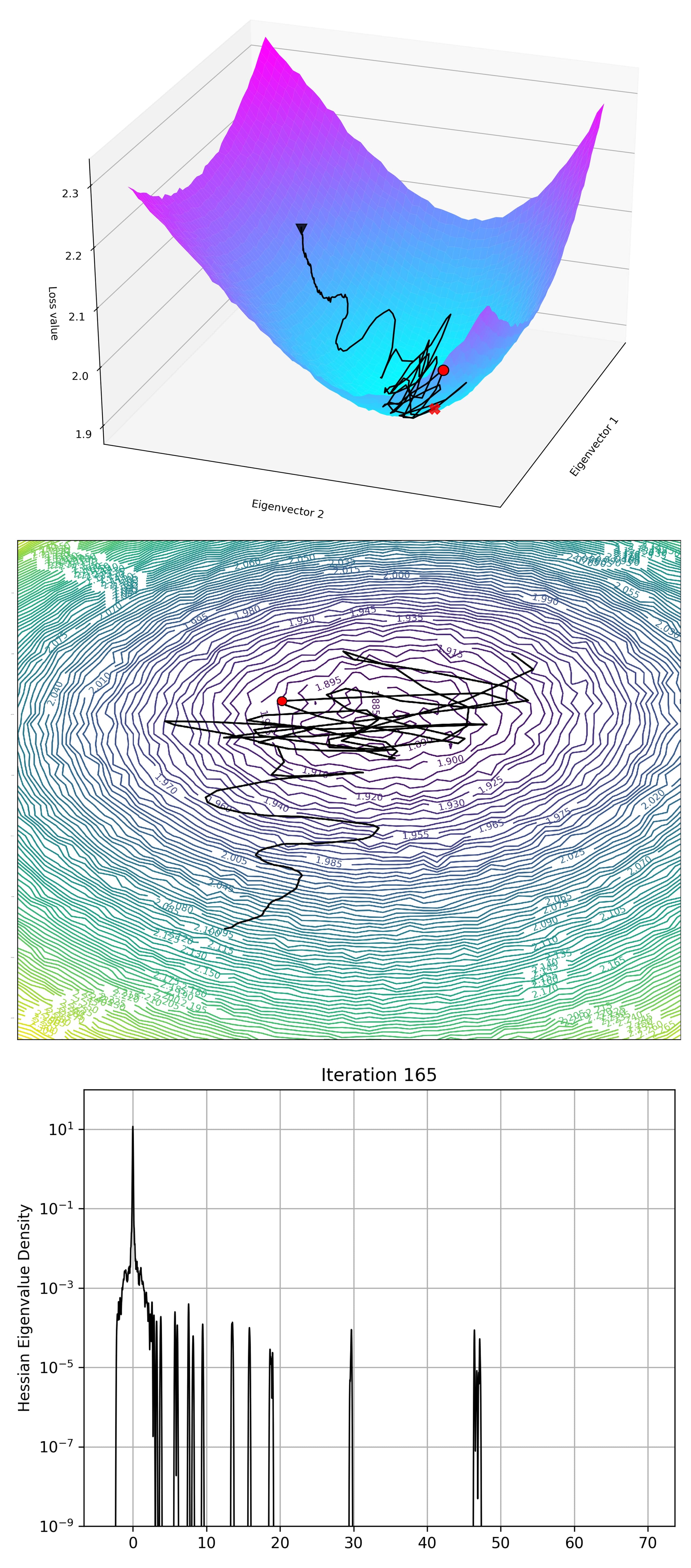
Figure 1: Using GradVis to plot the 3D and 2D Loss landscape, full gradient trajectory and eigenvalue density of the Hessian for a single iteration. Example shows a LeNet training on CIFAR10. Video of this visualization over all ittertions is available at: https://youtu.be/0AKSjp-SHlo

These seemingly contradicting results can be explained by their different approaches to measure flatness. [6] showed that one can reparametrize the loss function, thereby altering the geometry of the parameter space without affecting how the network evaluates unseen data. Hence, one can simply reparametrize the weights in a neural network layer without changing the value of the loss function.
This current discussion shows, that it is necessary to gain further theoretical insights into these optimization problems. A crucial contribution to such efforts could come from tools for the visualization and high resolution quantification of loss surface properties during the training process.

1.1 Related Work I: Loss surface visualization

First attempts to visualize loss landscapes were presented by [9]. The authors drew samples along a line in weight space, connecting the initialization point to the converged minimum. Along this line, the loss is calculated and plotted. As one result of their experiments, they were able to show that the loss along this line follows a monotonically decreasing path. [17] introduced a new method on how to visualize the loss landscape. Their main contribution is to use filter-wise normalization to combat the scaling invariance of the weights. The authors also use a PCA [21] on the training paths, reducing the problem onto a 2D plane. The landscape is then plotted by spanning a plane in parameter space around the converged point $\theta^{*}$ and taking the loss $L(\theta)$ at each point on this plane. Since PCA’s complexity is cubic, both in the number of samples and their dimensionality, and comes with high memory demands, it is quite difficult to implement this approach for larger networks. Additionally, this approach has been criticised by [2], who showed that performing PCA on high-dimensional random walks always results in Lissajous trajectories. They argue that the training trajectory, if plotted using PCA, always performs the same patterns, thereby rendering the information one can extract from the trajectory useless.

1.2 Related Work II: Second order properties of the loss surface

Another approach to gain further insight into the loss landscape is to compute the eigenvalues of the Hessian at different points in parameter space. The eigenvalues of the Hessian are a measure of curvature of the loss landscape. Positive eigenvalues correspond to positive curvature along its corresponding eigenvector, meaning the network is inside a minimum in this direction. Also its magnitude corresponds to how steep this minimum is. Calculating the eigenvalues of the Hessian of a neural network has a complexity of $O(N^{3})$. For regular networks with parameters in the range of $10^{6}-10^{8}$, this is infeasible to compute. Especially for all of the usual $10^{5}$ evaluations points during the iterations of the optimization process. Therefore, in order to compute the full eigenvalue spectrum, we adopt two common compute ”tricks” from other fields: First we are able to compute the Hessian-vector product efficiently in $O(N)$ instead of $O(N^{2})$ without having to store the Hessian during this process. This is done by using the R-operator [20], which is a linear operator that wraps around the forward and backward propagation in order to compute the Hessian-vector product. Second, by using the Lanczos algorithm [16], it only requires the Hessian-vector product to compute the eigenvalues. As [8] shows, one can approximate the full eigenvalue spectrum by only performing $m$ Lanczos iteration steps and by then diagonalizing the resulting $m\times m$ tridiagonal matrix. This procedure is done $k$ times with different starting vectors. Using the resulting eigenvalues and eigenvectors of this tridiagonal matrix, one can approximate the full eigenvalue spectrum using Gaussians to high accuracy in only $O(Nmk)$. The first paper to apply this method for neural networks was [18]. Through out this paper, we largely follow the notation of [7], using the stochastic Lanczos quadrature algorithm.

1.3 Contribution

In this paper, we present an open source toolbox for Python which is both compatible with Tensorflow [1] and PyTorch [19], introducing and implementing efficient and scalable algorithms for the analysis of loss surfaces during the training of deep neural networks. GradVis enables the user to visualize the trajectory of their model as well as the loss landscape and the eigenvalues of its Hessian. We propose efficient mathematical formulations of the key operators and a novel parallelization scheme that allows the investigation of the optimization process using practically relevant neural networks. First experiments show how the combination of visualizing the loss landscape and plotting the eigenvalue density spectrum leads to further insights into DNN training. In detail, our contributions are:

• Implementing efficient mathematical formulations for the computation of the Eigenvalue spectrum of the Hessian, reducing the complexity.

• Introducing a novel method-parallelization computation of the Eigenvalue spectrum, improving the parallel efficiency from $37\%$ of a data-parallel approach to over $96\%$

• We propose a solution to finding good directions in the high dimensional loss landscape for visualization, solving the problem of using a PCA for the approximation of the trajectory, as discussed in [2].

• Using our fast methods, we conducted several experiments that were (to our best knowledge) not possible before:

  • Computing the eigenvalue density spectrum at every iteration, crating high resolution videos of the trajectories and second order information while training a neural network.

  • Plotting a high resolution loss landscape in between two minima and analysing the eigenvalue density spectrum at all intermediate points

2 Methods

2.1 Filter-wise Normalization for Visualization

The Toolbox visualizes loss landscapes by projecting it onto two directional vectors in parameter space $\phi_{1}$ and $\phi_{2}$. It normalizes them and plots the loss along the plane that is spanned by those directions:

$$L(\theta_{n}+\alpha\phi^{*}_{1}+\beta\phi^{*}_{2})$$ (1)

where $\theta_{n}$ corresponds to the converged point in weight space.

Following [17], the Visualization Toolbox performs filter-wise normalization on the weights of the network to overcome the scale invariance of the parameter space. Given weights of a convolutional filter $\theta_{ij}$, filter wise-normalization performs the following operation:

$$d_{ij}^{*}=\frac{d_{ij}}{\left\lVert d_{ij}\right\rVert}\left\lVert\theta_{ij}\right\rVert$$ (2)

where $d_{ij}$ are the convolution weights of the directional vector $d$ and $d_{ij}$ corresponds to the jth filter for the ith convolution inside the neural network. $\left\lVert.\right\rVert$ corresponds to the Frobenius norm. The directional vector $d$ is either a random Gaussian vector, a custom vector provided by the user or it is calculated using principal component analysis (PCA) over all the saved iterations. All batch-norm parameters are set to zero.

PCA is a dimensionality reduction method. It allows finding the direction and magnitude of maximum data variation to the inverse of the covariance matrix [4]. The Toolbox can perform a PCA over the training runs $\left(\theta_{1},...,\theta_{n}\right)$ where $\theta_{i}$ are the networks weights at a certain iteration. We obtain the first two PCA directions $\phi_{1}$ and $\phi_{2}$.

The pseudocode is described in Algorithm 1.

Algorithm 1 Calculate the loss landscape for a neural network with loss $L$ for the n weights along the trajectory $(\theta_{1},...,\theta_{n})$. The resulting 2D landscape has N points along each axis on the grid

0:  Weights $(\theta_{1},...,\theta_{n})$

  Calculate the PCA vectors

  $\phi_{1}$,$\phi_{2}$ $\leftarrow$ PCA($\theta_{1}-\theta_{n},...,\theta_{n-1}-\theta_{n}$)

  Use filter-wise normalization

  $\phi^{*}_{1}$ $\phi^{*}_{2}\leftarrow$ Normalize($\phi_{1},\phi_{2}$)

  Calculate the coefficients of the training path

  $\alpha_{i},\beta_{i}\leftarrow$ Solve for $\alpha_{i}\phi^{*}_{1}+\beta_{i}\phi^{*}_{2}=\theta_{i}-\theta_{n}$ for each i

  Calculate the loss values of the path points

  $z_{i}\leftarrow L(\alpha_{i}\phi^{*}_{1}+\beta_{i}\phi^{*}_{1}+\theta_{n})$

  Calculate the loss values for each point on the grid

  Make grid of N samples going from $min(\alpha_{i})$ to $\max(\alpha_{i})$ for x and $min(\beta_{i})$ to $\max(\beta_{i})$ for y

  for i from 0 to N do

     for j from 0 to N do

        $x=i(max(\alpha)-\min(\alpha))/N$

        $y=j(max(\beta)-\min(\beta))/N$

        $z_{i,j}\leftarrow L(x\phi^{*}_{1}+y\phi^{*}_{2}+\theta_{n})$

     end for

  end for

  return  ($z_{1,1},...,z_{N,N}$)

2.2 Stochastic Lanczos quadrature algorithm

The stochastic Lanczos quadrature algorithm [16] is a method for the approximation of the eigenvalue density of very large matrices. The eigenvalue density spectrum is given by:

$$\phi(t)=\frac{1}{N}\sum_{i=1}^{N}\delta(t-\lambda_{i})$$ (3)

where $N$ is the number of parameters in the network and $\lambda_{i}$ is the i-th eigenvalue of the Hessian.

The eigenvalue density spectrum is approximated by a sum of Gaussian functions:

$$\phi_{\sigma}(t)=\frac{1}{N}\sum_{i=1}^{N}f(\lambda_{i},t,\sigma^{2})$$ (4)

where

$$f(\lambda_{i},t,\sigma^{2})=\frac{1}{\sigma\sqrt{2\pi}}\exp(-\frac{(t-\lambda_{i})^{2}}{2\sigma^{2}})$$ (5)

We use the Lanczos algorithm with full reorthogonalization in order to compute eigenvalues and eigenvectors of the Hessian and to ensure orthogonality between the different eigenvectors. Since the Hessian is symmetric we can diagonalize it. All eigenvalues will be real. The Lanczos algorithm returns a tridiagonal matrix. This matrix is diagonalized:

$$T=ULU^{T}$$ (6)

By setting $\omega_{i}=(U_{1,i}^{2})_{i=1}^{m}$ and $l_{i}=(L_{ii})_{i=1}^{m}$, the resulting eigenvalues and eigenvectors are used to estimate the true eigenvalue density spectrum:

$$\hat{\phi}^{(v_{i})}(t)=\sum_{i=1}^{m}\omega_{i}f(l_{i},t,\sigma^{2})$$ (7)

$$\hat{\phi}_{\sigma}(t)=\frac{1}{k}\sum_{i=1}^{k}\hat{\phi}^{(v_{i})}(t)$$ (8)

The pseudocode for the stochastic Lanczos quadrature algorithm is shown in Algorithm 2.

Algorithm 2 Stochstic Lanczos quadrature algorithm

0:  Number of iterations k, number of eigenvalues m

  Initialize Guassian vectors $(v_{1},...,v_{k})$

  for i from 1 to k do

     Run Lanczos with reothogonalization with $L(v_{i})$

     Obtain tridiagonal matrix T

     Diagonalize $T=ULU^{T}$

     Set $l_{i}=(L_{ii})_{i=1}^{m}$ and $\omega_{i}=(U_{1,i}^{2})_{i=1}^{m}$

     Compute $\hat{\phi}^{(v_{i})}(t)=\sum_{i=1}^{m}\omega_{i}f(l_{i},t,\sigma^{2})$

  end for

  Compute average $\hat{\phi}_{\sigma}(t)=\frac{1}{k}\sum_{i=1}^{k}\hat{\phi}^{(v_{i})}(t)$

  return  $\hat{\phi}_{\sigma}(t)$

2.3 Parallelization

Data-Parallel Visualization. The visualization method is trivially parallelizable by assigning parts of the evaluation grid to different workers. After each worker is done computing its values, the master-worker collects the values of each worker using MPI_Gatherv. The peudocode for the parallelized version is shown in Algorithm 3.

Algorithm 3 Parallel visualization method. Calculate the loss landscape for a neural network with loss $L$ for the n weights along the trajectory $(\theta_{1},...,\theta_{n})$. The resulting 2D landscape has N points along each axis on the grid

0:  Weights $(\theta_{1},...,\theta_{n})$

  Calculate the PCA vectors

  $\phi_{1}$,$\phi_{2}$ $\leftarrow$ PCA($\theta_{1}-\theta_{n},...,\theta_{n-1}-\theta_{n}$)

  Use filter-wise normalization

  $\phi^{*}_{1}$ $\phi^{*}_{2}\leftarrow$ Normalize($\phi_{1},\phi_{2}$)

  Calculate the coefficients of the training path

  $\alpha_{i},\beta_{i}\leftarrow$ Solve for $\alpha_{i}\phi^{*}_{1}+\beta_{i}\phi^{*}_{2}=\theta_{i}-\theta_{n}$ for each i

  Calculate the loss values of the path points

  $z_{i}\leftarrow L(\alpha_{i}\phi^{*}_{1}+\beta_{i}\phi^{*}_{1}+\theta_{n})$

  Calculate the loss values for each point on the grid

  Make grid of N samples going from $min(\alpha_{i})$ to $\max(\alpha_{i})$ for x and $min(\beta_{i})$ to $\max(\beta_{i})$ for y

  Split grid into m chunks according to number of workers m $X_{k}$,$Y_{k}$ for k = 1,…,m

  Assign each worker part of the grid

  for $x$ in $X_{k}$ do

     for $y$ in $Y_{k}$ do

        $z_{x,y}\leftarrow L(x\phi^{*}_{1}+y\phi^{*}_{2}+\theta_{n})$

     end for

  end for

  Each worker has set of values $Z_{k}$

  $Z$ $\leftarrow$ MPI_Gatherv($Z_{k}$)

  return  Z = ($z_{1,1},...,z_{N,N}$)

Data-Parallel Lanczos. The Lanczos algorithm only requires the Hessian-vector product instead of the full Hessian matrix in order to compute eigenvalues. This allows using the R-operator to calculate these products effieciently. Using MPI, we distribute the batches to different workers, where each worker accumulates its own Hessian-vector products by using the R-operator. After all workers are done computing their batches the resulting vectors are sent to the master-worker and summed by using the MPI_Reduce operation. The pseudocode is shown in Algorithm 4.

Algorithm 4 Data parallel Lanczos. Calculation of Hessian-vector products $Hv$ by using the R-operator

0:  vector $v$ and neural network model $h(x)$

  Set batch size B and therefore divide the dataset into p batches

  for i from 1 to p do

     Worker j grabs batch and starts computing the hessian vector product $w_{i}=R_{op}(h(b_{i}),v)$

  end for

  The resulting Hessian vector product gets accumulated during this loop for each worker $w_{j}=\frac{1}{|I_{j}|}\sum_{r\in I_{j}}w_{r}$ where $I_{j}$ contains the indices of batches that were computed for worker j

  Send all resulting $w_{j}$ to the master-worker using $w=MPI\_Reduce(w_{j})$

  return  Hessian vector product over all samples $w$

This data parallel approach allowed us to use far more samples in our eigenvalue spectrum computation. Future research could look into model parallelism as well, since the R-operator works exactly like a neural network with forward and backward propagation.

Novel Iteration-Parallel Lanczos. We introduce another approach to parallelize the Lanczos method, that proved to be much more scalable. The basic idea is to let each worker compute one iteration of the stochstic Lanczos quadrature algorithm for different initializations and then accumulating all the results at the end on the master-worker. This approach can be seen in Algorithm 5.

Algorithm 5 Parallel stochstic Lanczos quadrature algorithm with MPI

0:  Number of iterations k, number of eigenvalues m

  Initialize Guassian vectors $(v_{1},...,v_{k})$ and split this set to $s$ different workers

  for $v_{i}$ from the set assigned to each worker do

     Run Lanczos with reothogonalizationon on worker w with $L(v_{i})$

     Obtain tridiagonal matrix T

     Diagonalize $T=ULU^{T}$

     Set $l_{i}=(L_{ii})_{i=1}^{m}$ and $\omega_{i}=(U_{1,i}^{2})_{i=1}^{m}$

  end for

  Each worker sends its computed $l_{i}$ from all different initializations to the master-worker using MPI_Gatherv. The same is done for the $\omega_{i}$

  Compute average on the master-worker $\hat{\phi}_{\sigma}(t)=\frac{1}{k}\sum_{i=1}^{k}\sum_{i=1}^{m}\omega_{i}f(l_{i},t,\sigma^{2})$

  return  $\hat{\phi}_{\sigma}(t)$

3 Experiments

3.1 Timing and Scalability

As seen in Algorithm 1, the toolbox evaluates the network on the training samples $N^{2}$ times, where N is the number of points on the grid along the x- and y-axis. On each grid point, the network evaluates $n_{b}$ batches and the evaluation of each batch takes time $T_{inference}$. Hence, the time to evaluate all the grid points is of the order of $\alpha+N^{2}T_{inference}n_{b}$, with some overhead $\alpha$ for the computation of the PCA components, as well as for performing the filter-wise normalization. But this overhead is small for large enough $N$. For example, performing experiments with a Resnet-32 for a batch size of 256 and 2 batches resulted in $\alpha=8s$ and $T_{inference}=0.005s$. Table 1 shows, that the overhead $\alpha$ stays constant while computation time for the loss landscape scales like $N^{2}$

Table 1: Timing of loss landscape calculation and overhead for different N

Timing in seconds
	N=2	N=10	N=50	N=100
$N^{2}T_{inference}n_{b}$	0.51	12.72	320	1890
$\alpha$	8.21	8.01	8.09	8.11

Scalability. The scalability is measured by measuring the speedup given by

$$S=\frac{T_{1}}{T_{p}},$$ (9)

where $T_{1}$ is the time for one process and $T_{p}$ the time for $p$ processes. In our setting each node contains two Nvidia GTX 1080ti GPUs and they are assigned sequentially by first filling one node and then populating the next node with increasing number of ranks. The standard deviation on the datapoints is calculated as follows:

$$\sigma_{s}=\sqrt{(\frac{1}{T_{p}})^{2}\sigma_{T_{1}}^{2}+(\frac{T_{1}}{T_{p}^{2}})^{2}\sigma_{T_{p}}^{2}}$$ (10)

We measure strong scaling by keeping the problem size fixed and varying the number of GPUs, computing the parallelizable fraction according to Amdahls law:

$$S=\frac{1}{(1-f)+f/p},$$ (11)

where $f$ is the parallelizable fraction of our implementation and $p$ refers to the number of GPUs working in parallel on the problem. For the stochstic Lanczos quadrature algorithm presented in Algorithm 5, the scaling plot is shown in Figure 2. One can see that fitting Formula 11 to our data we obtain a parallelizable fraction of $f=95.5\pm 0.4\%$. Comparing this to the data parallel approach, here we obtain the strong scaling plot in Figure 2.

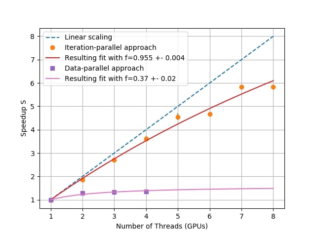
Figure 2: Strong scaling plot for the stochastic Lanczos quadrature algorithm with data parallelism and with our proposed method.

Fitting the model yields a parallelizable fraction of $f=37\pm 2\%$, which much is worse than our novel method.

For the visualization presented in Algorithm 3, we obtain Figure 3.

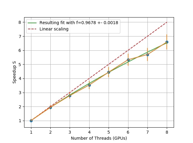
Figure 3: Strong scaling plot for the visualization algorithm.

Here we see that we get a parallelizable fraction of $f=96.78\pm 0.18\%$. Due to the trivially parallelizable nature of the algorithm at hand, the parallelizable fraction is very high.

3.2 Finding directions for Visualization

In order to circumvent the issue of using PCA on the training data (as discussed by [2]), we propose using different eigenvectors to plot the loss landscape together with the trajectory. Here we make use of the Lanczos algorithm that we combined with the R-operator in order to efficiently compute Hessian-vector products. Since the Lanczos algorithm is an iterative eigenvalue solver we are able to pick certain eigenvectors we are interested in. Therefore, instead of choosing random directions or PCA directions we propose using eigenvectors in order to visualize the training trajectory on the loss landscape. We compare the different methods to find directions in order to plot the trajectory. First we choose two randomly initialized vectors with entries drawn from a normal distribution. The resulting plot is shown in Figure 6.

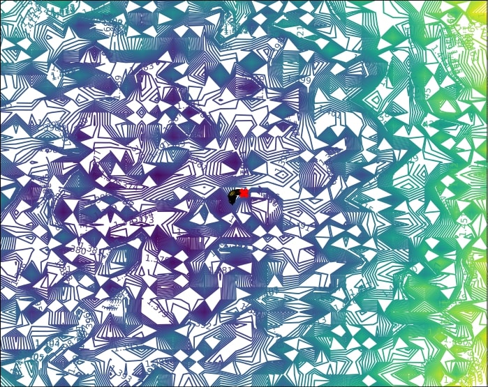
Figure 4: Loss landscape with trajectory along two random directions for LeNet on CIFAR10.

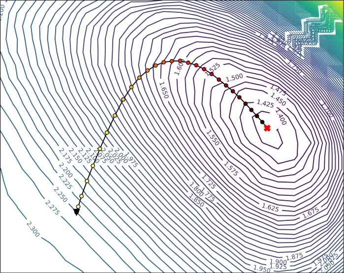
Figure 5: Loss landscape with trajectory of the same training run, visualized along two PCA directions with highest variance for LeNet on CIFAR10, as suggested by [17].

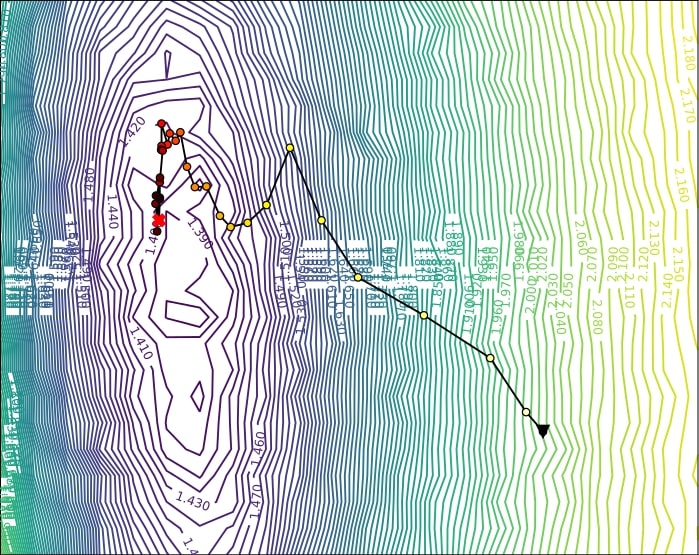
Figure 6: Loss landscape with trajectory of the same training run, visualized along eigenvectors corresponding to the two highest eigenvalues for LeNet on CIFAR10.

Next we use PCA to extract the two directions with the highest variance. The resulting visualization is shown in Figure 6. Lastly we use our proposed method of choosing eigenvectors to plot the trajectory. Here we choose the eigenvectors corresponding to the highest two eigenvalues. The resulting plot can be seen in Figure 6.

We can see how the random direction method in Figure 6 provides little to no information on what happens during training. The loss landscape is very noisy and relatively flat, the training path barely moves from its initial position.

On the contrary, the PCA directions show the trajectory spiraling into the minimum, which is clearly visible. The path that the trajectory takes is exactly what one would expect [2], if a PCA is taken on a high-dimensional random walk with drift. Therefore even though it seems that the trajectory offers insight into the training procedure, in reality we will always get the same trajectory, thereby rendering this method useless.

Our proposed method on the other hand, shows how the trajectory moves along the gradient and after reaching the valley slowly creeps towards the minimum. This method also allows picking interesting eigenvalues where our network seems to ”fail” during training, such as negative or zero eigenvalues. This allows monitoring what the training trajectory was doing in these directions.

3.3 Loss Landscape with Trajectory and Eigenvalue Density for LeNet

We present the loss landscape together with the trajectory of a LeNet architecture that is trained on CIFAR10 [15]. The neural network is trained for 1 epoch with 196 iterations with a batch size of 256 and a learning rate of 0.001, using SGD. Also a momentum of 0.9 is used. After each iteration the weights of the model are saved onto the hard drive.

For visualization a grid size of N=50 is used with an additional border of 40 % around the trajectory. The evaluation uses $20\%$ of all the samples in the training set. The loss landscape is plotted along the two eigenvectors corresponding to the two highest eigenvalues of the Hessian. For the eigenvalue density plots $k=10$ iterations were used and $m=80$ iterations were performed in the Lanczos algorithm. Also 20% of the CIFAR10 samples were used. The resulting plots are shown in Figure 7. These only show a select number of plots out of the 196 generated .

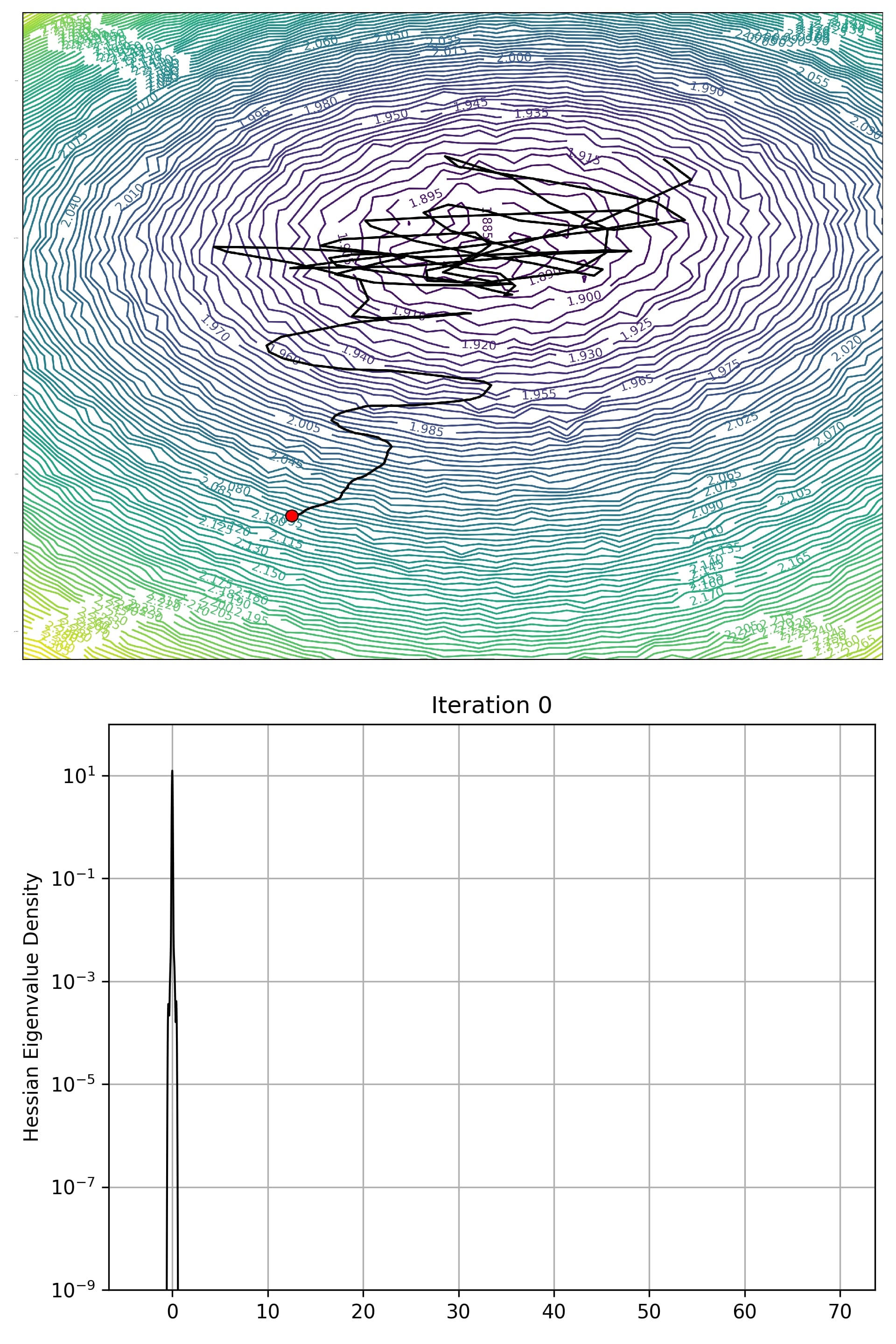
(a) Loss landscape and eigenvalue density plot of LeNet at initialization.

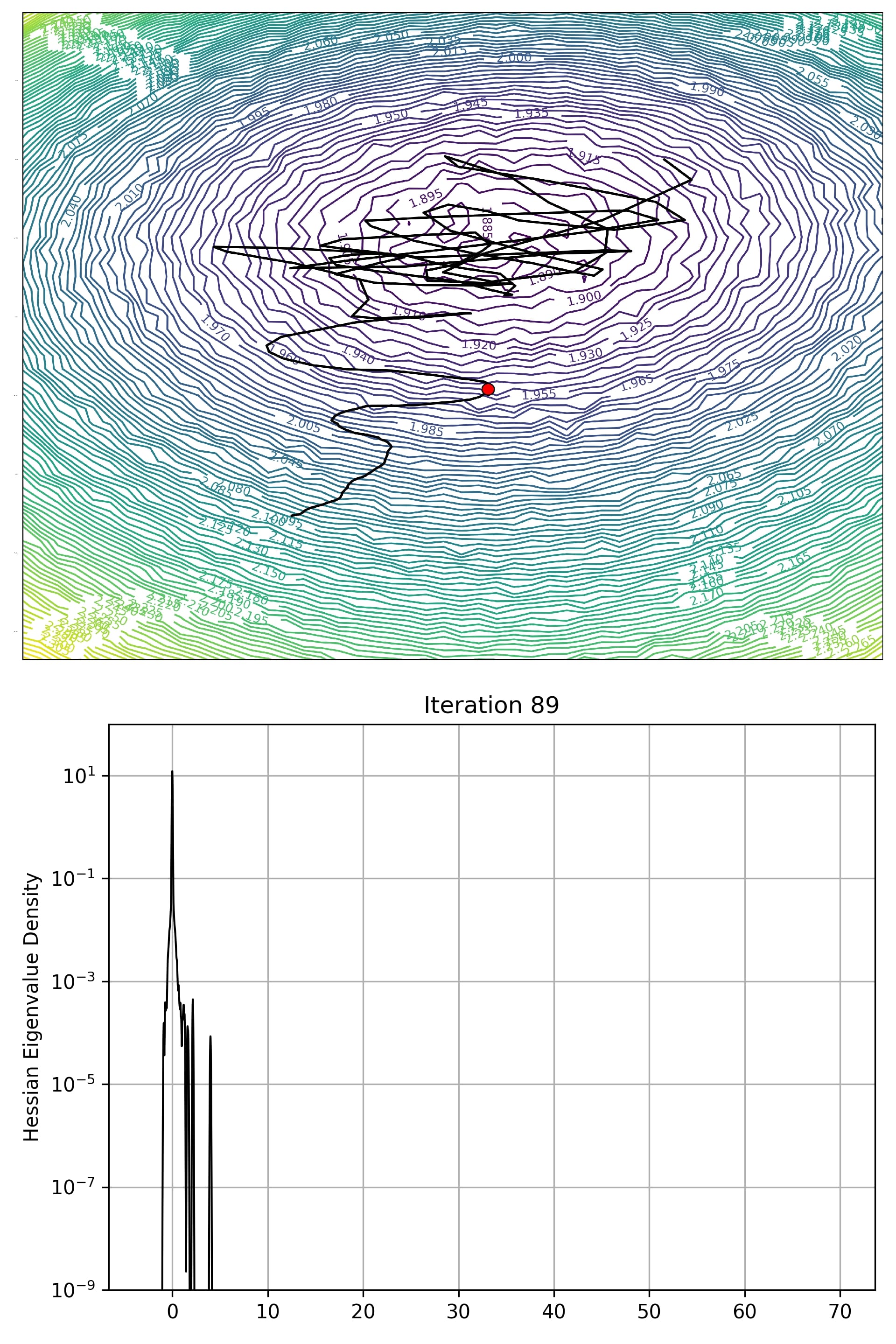
(b) Loss landscape and eigenvalue density plot of LeNet. Same training run at 89 iterations.

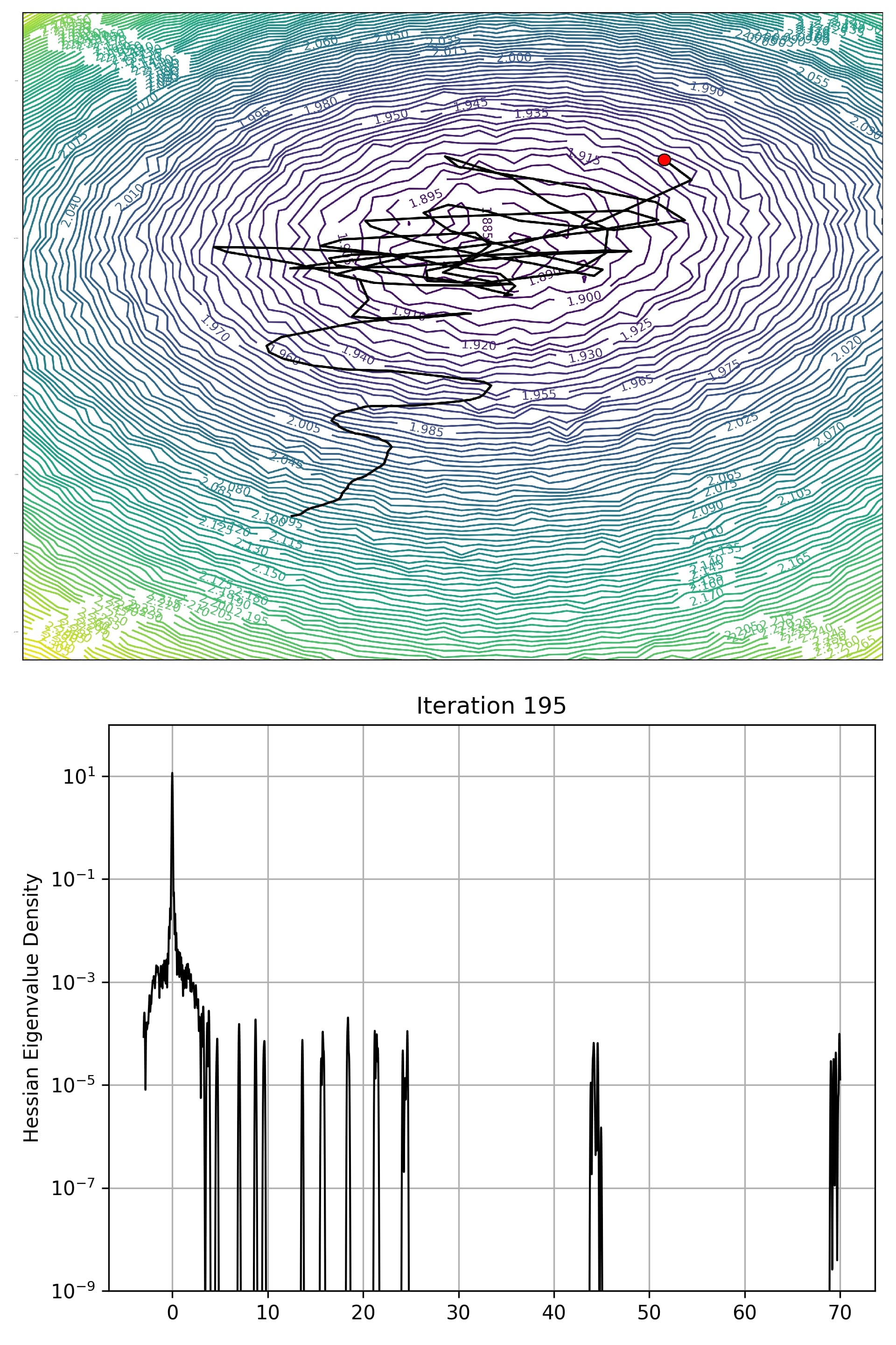
(c) Loss landscape and eigenvalue density plot of LeNet. Same trainig run at 195 iterations.

Figure 7: Loss landscape and Hessian eigenvalue density for three out of 195 iterations. Here a LeNet architecture is trained in CIFAR10 with using SGD with momentum. A learning rate of 0.01 was used as well as a momentum of 0.9. Both plots were generated using 20 % of the training samples. The visualization is depicted along two eigenvectors corresponding to the two highest eigenvalues of the Hessian. The plot has a grid size of 50 on each side.

At the beginning, during initialization the network finds itself inside a relatively flat saddle point with all eigenvalues being almost zero. The network struggles to escape this flat saddle point, it only manages to converge towards minima in some directions after 89 iterations, as seen in Figure 7(b).

One can see in Figure7(c), at the end of the first epoch after 196 iterations, the network has converged into minima in some dimensions, while overall the network still sits on a saddle point. The bulge on eigenvalues around zero has spread out a little bit more, meaning that in some dimensions the network sits at a maximum. Looking at the loss landscape, the network converged into a minimum in the depicted two dimensions. The trajectory oscillates around the minimum and it looks like the trajectory is about to escape the minimum again, which could be due to the fixed learning rate and the momentum which was used in SGD. Also, it seems that the loss landscape is convex in this area.

3.4 Interpolation in between two minima

We train a LeNet network two times with different initializations on CIFAR10, using a SGD optimizer with a learning rate of $lr=0.01$ and a momentum of $m=0.9$. The batch size is $b=256$ and the network is trained for 10 epochs. The resulting minima are plotted using the visualization method with a grid size of $N=50$ and 20% of all samples. Both minima are connected by a straight line. We extract 20 points along the line connecting both minima. Using the stochastic lanczos quadrature with the same parameters as in section 3.3, we obtain Figure 8.

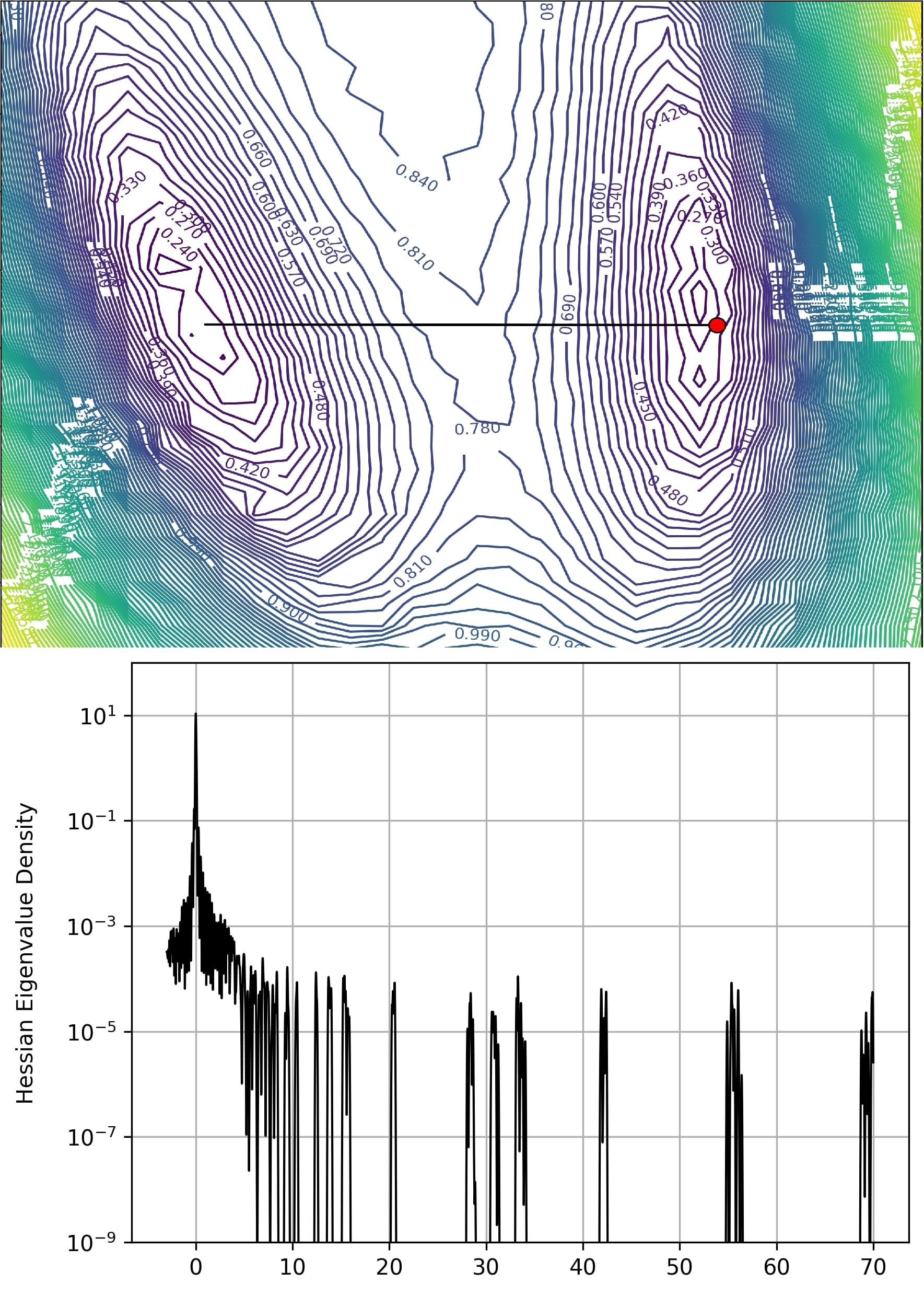
(a) Interpolation between 2 minima with eigenvalue density spectrum in minimum 1

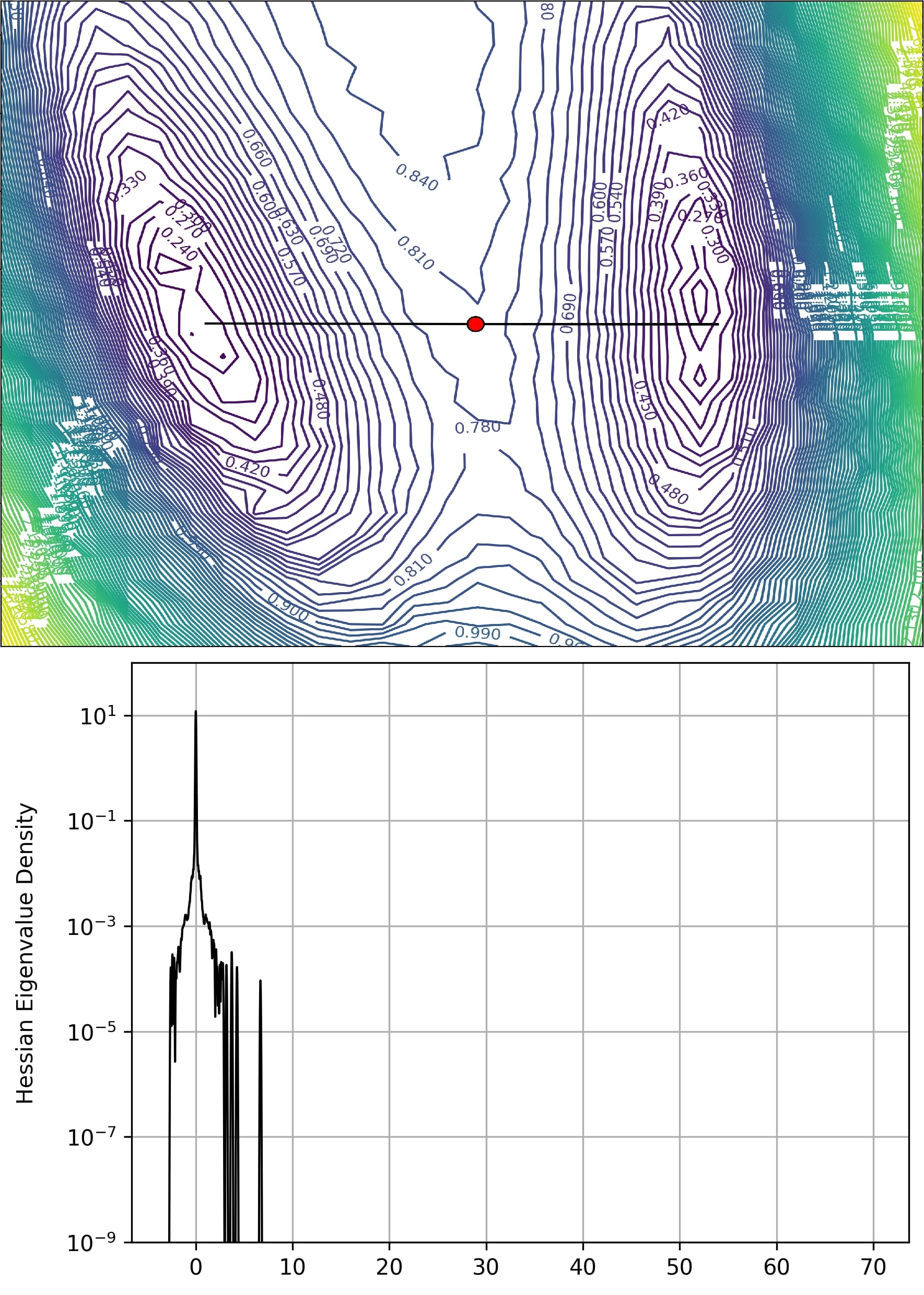
(b) Interpolation between 2 minima with eigenvalue density spectrum in between those

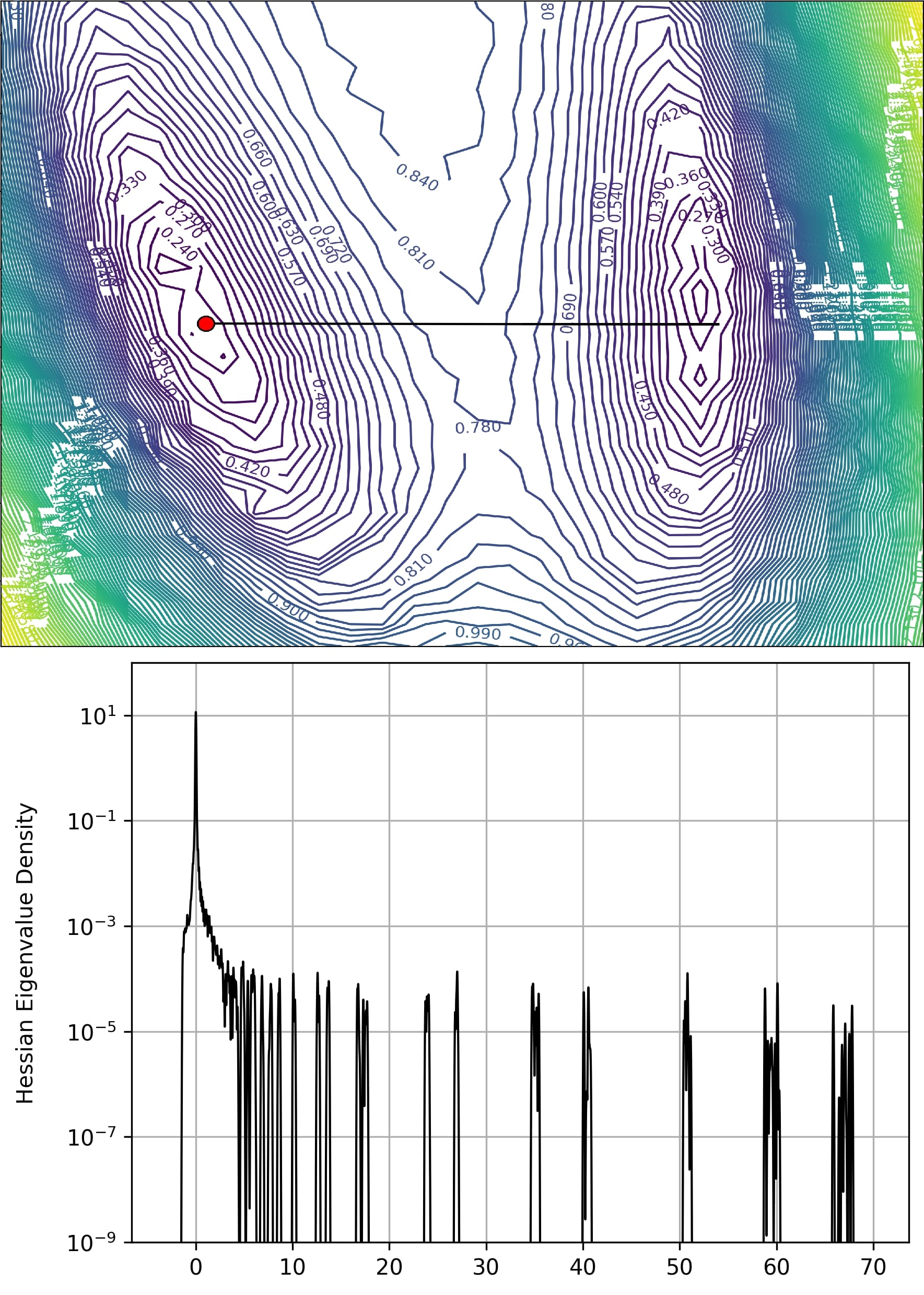
(c) Interpolation between 2 minima with eigenvalue density spectrum in minimum 2

Figure 8: Visualization of the loss landscape and the Hessian eigenvalue density at different points on the line connecting both minima. A LeNet architecture has been trained with two different initializations to end up in two different minima. For both plots 20 % of the CIFAR10 training samples were used. The loss landscape plot was crated with a grid size of 50 on each side.

As show in Figure 8, the eigenvalues inside both minima indicate, that the network is sitting on a saddle point, as there are always small negative eigenvalues present. Also there are a few eigenvalues that are much bigger, indicating a sharp minimum in the corresponding eigenvector directions. Going toward the middle of the interpolation those big eigenvalues shift back towards zero. This shows that in between those minima we are still in a saddle point but there is no big maximum that separates them, which would be indicated by large negative eigenvalues.

4 Discussion

Looking at the training of a LeNet architecture during its first epoch in Figure 7, one can observe that the network starts off at a flat saddle point and only gradually falls into minima in some directions. In most directions the network has zero eigenvalues and some are also negative. The negative eigenvalues also get more negative during training, which indicates that the network is located on a maximum in the direction of the corresponding eigenvector.

Comparing the different methods to plot the loss landscape together with the trajectory, we see that choosing random directions result in plots that show little to no information. Here the trajectory barely moves away from its initial position. The PCA directions seem to offer a good choice to plot the trajectory. But PCA actually chooses its directions in such a way that one always obtains the same figure of the trajectory. Therfore this method is insufficient in offering any useful information of the training procedure. On the other hand, one can see that choosing eigenvectors results in interesting directions where minima as well as trajectories are present. Here the trajectories always look different and represent the ”true” path taken by the optimizer. Looking at the eigenvalues of the interpolation between two different minima in Figure 8 one can observe that the area in between those two minima is relatively flat. Most positive eigenvalues get pushed toward zero while the negative ones are not changing by a lot compared to the minima. Also looking at the scalability of the algorithms, we see that the visualization method is highly parallelizable, this is to be expected as we are able to split the grid and each worker can compute its values independently. For the stochastic Lanczos quadrature algorithm our algorithm is also highly parallelizable, again this is possible because the different initializations in the outer loop of the algorithm are independent of each other. On the other hand, using data parallelism in this algotrithm is much less parallelizable. One reason could be that after each time the dataset has been computed, all GPUs have to wait on the algorithm to finish the rest of the computations for this iteration. Still, if one attempts to scale to hundreds of GPUs, the best approach would be to perform a mix of both approaches, as the number of independent iterations in the stochastic Lanczos quadrature algorithm is on a scale of $10^{1}$. So using more GPUs than iterations to compute would make no sense, therefore the remaining ones could compute samples in a data parallel fashion.

5 Conclusion

The presented GradVis tool box now makes it feasible to compute high resolution (in terms of optimization space and iterations) visualizations of the loss surfaces, gradient trajectories and eigenvalue spectra of the Hessians of full training runs of practically relevant deep neural networks. Especially our fast implementation and novel scalable parallelization of the Lanczos algorithm will make GradVis a valuable tool towards a better theoretical understanding of SDG based optimizations methods for deep learning. First experimental results already show very interesting insights. The next step for future work will be to compute full scale evaluations for large prominent networks on large data sets, like ResNet on ImageNet.

References

- [1] M. Abadi, A. Agarwal, P. Barham, E. Brevdo, Z. Chen, C. Citro, G. S. Corrado, A. Davis, J. Dean, M. Devin, S. Ghemawat, I. Goodfellow, A. Harp, G. Irving, M. Isard, Y. Jia, R. Jozefowicz, L. Kaiser, M. Kudlur, J. Levenberg, D. Mané, R. Monga, S. Moore, D. Murray, C. Olah, M. Schuster, J. Shlens, B. Steiner, I. Sutskever, K. Talwar, P. Tucker, V. Vanhoucke, V. Vasudevan, F. Viégas, O. Vinyals, P. Warden, M. Wattenberg, M. Wicke, Y. Yu, and X. Zheng. TensorFlow: Large-scale machine learning on heterogeneous systems, 2015. Software available from tensorflow.org.
- [2] J. Antognini and J. Sohl-Dickstein. Pca of high dimensional random walks with comparison to neural network training. In Advances in Neural Information Processing Systems, pages 10307–10316, 2018.
- [3] A. Blum and R. L. Rivest. Training a 3-node neural network is np-complete. In Proceedings of the First Annual Workshop on Computational Learning Theory, COLT ’88, pages 9–18, San Francisco, CA, USA, 1988. Morgan Kaufmann Publishers Inc.
- [4] M. Borga, T. Landelius, and H. Knutsson. A unified approach to pca, pls, mlr and cca. Linköping University, Department of Electrical Engineering, 1997.
- [5] P. Chaudhari, A. Choromanska, S. Soatto, Y. LeCun, C. Baldassi, C. Borgs, J. T. Chayes, L. Sagun, and R. Zecchina. Entropy-sgd: Biasing gradient descent into wide valleys. CoRR, abs/1611.01838, 2016.
- [6] L. Dinh, R. Pascanu, S. Bengio, and Y. Bengio. Sharp minima can generalize for deep nets. CoRR, abs/1703.04933, 2017.
- [7] B. Ghorbani, S. Krishnan, and Y. Xiao. An investigation into neural net optimization via hessian eigenvalue density. CoRR, abs/1901.10159, 2019.
- [8] G. H. Golub and J. H. Welsch. Calculation of gauss quadrature rules. Technical report, Stanford, CA, USA, 1967.
- [9] I. J. Goodfellow, O. Vinyals, and A. M. Saxe. Qualitatively characterizing neural network optimization problems. arXiv preprint arXiv:1412.6544, 2014.
- [10] G. E. Hinton and D. van Camp. Keeping the neural networks simple by minimizing the description length of the weights. In Proceedings of the Sixth Annual ACM Conference on Computational Learning Theory, COLT 1993, Santa Cruz, CA, USA, July 26-28, 1993., pages 5–13, 1993.
- [11] S. Ioffe and C. Szegedy. Batch normalization: Accelerating deep network training by reducing internal covariate shift. CoRR, abs/1502.03167, 2015.
- [12] S. Jastrzkebski, Z. Kenton, N. Ballas, A. Fischer, Y. Bengio, and A. Storkey. On the relation between the sharpest directions of dnn loss and the sgd step length. 2018.
- [13] N. S. Keskar, D. Mudigere, J. Nocedal, M. Smelyanskiy, and P. T. P. Tang. On large-batch training for deep learning: Generalization gap and sharp minima. CoRR, abs/1609.04836, 2016.
- [14] J. Kiefer and J. Wolfowitz. Stochastic estimation of the maximum of a regression function. Ann. Math. Statist., 23(3):462–466, 09 1952.
- [15] A. Krizhevsky, V. Nair, and G. Hinton. Cifar-10 (canadian institute for advanced research).
- [16] C. Lanczos. An iteration method for the solution of the eigenvalue problem of linear differential and integral operators. Journal of research of the National Bureau of Standards, 45, 255–282., 1950.
- [17] H. Li, Z. Xu, G. Taylor, and T. Goldstein. Visualizing the loss landscape of neural nets. CoRR, abs/1712.09913, 2017.
- [18] V. Papyan. The full spectrum of deep net hessians at scale: Dynamics with sample size. CoRR, abs/1811.07062, 2018.
- [19] A. Paszke, S. Gross, S. Chintala, G. Chanan, E. Yang, Z. DeVito, Z. Lin, A. Desmaison, L. Antiga, and A. Lerer. Automatic differentiation in pytorch. In NIPS-W, 2017.
- [20] B. A. Pearlmutter. Fast exact multiplication by the hessian. Neural Computation, 6:147–160, 1994.
- [21] K. Pearson. Liii. on lines and planes of closest fit to systems of points in space. Nov 1901.