From classical to modern opinion dynamics

Abstract

In this age of Facebook, Instagram, and Twitter, there is rapidly growing interest in understanding network-enabled opinion dynamics in large groups of autonomous agents. The phenomena of opinion polarization, the spread of propaganda and fake news, and the manipulation of sentiment is of interest to large numbers of organizations and people. Whether it is the more nefarious players such as foreign governments that are attempting to sway elections or it is more open and above board, such as researchers who want to make large groups of people aware of helpful innovations, what is at stake is often significant.

In this paper, we review opinion dynamics including the extensions of many classical models as well as some new models that deepen understanding. For example, we look at models that track the evolution of an individual’s power, that include noise, and that feature sequentially dependent topics, to name a few.

While the first papers studying opinion dynamics appeared over 60 years ago, there is still a great deal of room for innovation and exploration. We believe that the political climate and the extraordinary (even unprecedented) events in the sphere of politics in the last few years will inspire new interest and new ideas.

It is our aim to help those interested researchers understand what has already been explored in a significant portion of the field of opinion dynamics. We believe that in doing this, it will become clear that there is still much to be done.

Keywords:— Opinion game, opinion dynamics, social dynamic, social interaction, consensus, polarization

1 Introduction

The problem with studying human relational dynamics mathematically is that as soon as we present such phenomena in a way that is amenable to mathematical analysis, we have stripped away much of the nuance and, more importantly, the complexity that exist in the real world. Of course, this is also a benefit, since it is impossible to represent such systems in their full complexity. Therefore, the art of modeling consists in performing this reduction in a way that leaves something of value intact.

However, carefully crafted models can provide useful insights into how real human systems work.

In our case, we want to understand the dynamics of opinions in groups of people who interact with each other and a context of information – what causes people to change opinions and groups that support or oppose an opinion to gain or lose influence and power? This is, of course a very old topic of interest. As long as there has been groups of people whose opinions differed (and mattered), this has been of interest.

In this paper we review a partial cross section of the mathematical approaches to answering these questions. While these models are all radically simplified representation of the social and economic systems, what has been done is at least provacative and interesting. The idea that we can mathematically model and study the evolution of opinions is not a new one - research using a mathematical perspective dates back at least as far as John R. P. French’s 1956 paper A Formal Theory of Social Power[1]. More recently, but still many decades old, is the work of DeGroot in 1974[2] and Friedkin in 1986[3].

1.1 Mathematical Representation

When modeling opinions and their dynamics we must, at a minimum, represent the opinions that are held as well as the means by which people interact, both influencing and being influenced. We also need to choose how we represent time.

Opinion Spaces

Opinions can be represented by both discrete variables as well as by continuous representations. For example, in a two-party election, we might represent opinions by a discrete variable, candidate $A$ or candidate $B$ (Fig. 1(a)). In contrast, while designing a new product, we might care about the distribution of prices that customers are willing to pay, which we might represent by real numbers in the interval $[0,1]$ (Fig. 1(b)), $0$ representing some minimal amount and $1$ the maximal potential price. It is possible that one opinion be presented via an ordered pair (Fig. 1(c)). If one wants to choose a favorite color based on combination of red, green and blue then the opinion space can be the unit cube (Fig. 1(d)). In this paper, we focus our attention on models of opinion spaces as intervals in $\mathbb{R}$.

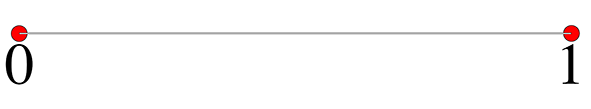
(a) binary opinion space

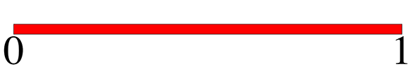
(b) continuous 1D opinion space

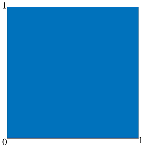
(c) 2D opinion space

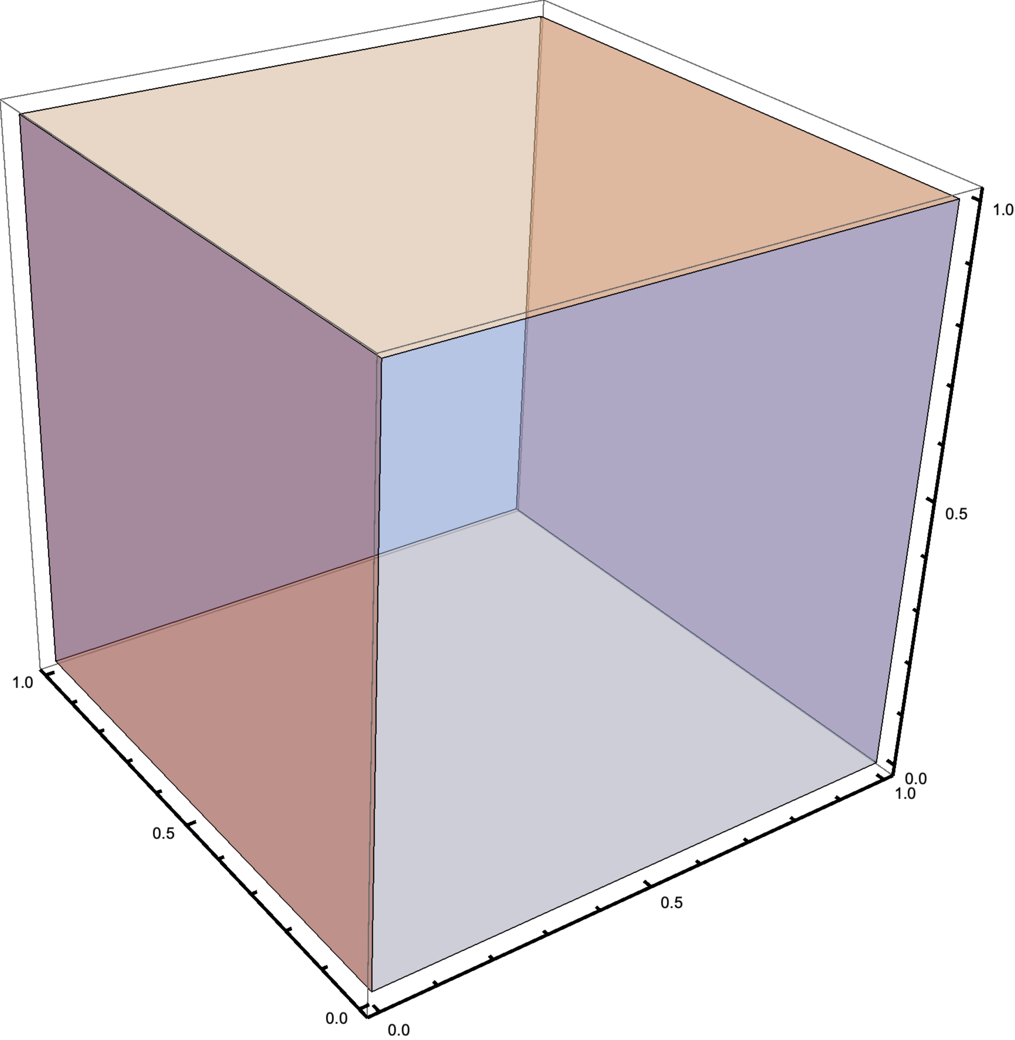
(d) a cubical opinion space

Figure 1: opinion space examples. In Fig. 1(a) the opinions are binary either 0 or 1, in Fig. 1(b) opinions are continuous anywhere between 0 and 1, and Fig. 1(c) is a two dimensional opinion space, it could also be a triangle or a simplex.

Interactions

A natural starting place for the representation of interactions is a network, with a node for each person (we will call them agents) and an edge, representing pairwise interactions between each pair of agents. If we have $N$ people each with an opinion, then there will be $\frac{N*(N-1)}{2}$ pairs of people and possible interactions, assuming we focus on pairwise interactions. The result is a network with $N$ nodes and $\frac{N*(N-1)}{2}$ possible edges, each perhaps with a weight or even two weights for influence if there is an asymmetry in persuasiveness. If a pair of agents have different influences on each other then the relations are defined by directed edges (Fig. 2(b)) and in this case the complete-graph will have $N*(N-1)$ directed edges. Of course, the agents can also be media entities, in which case it is clear that there would typically be an asymmetry in influence where a directed graph can be used (Fig. 2(b)).

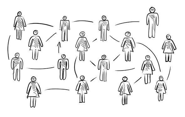
(a) undirected network

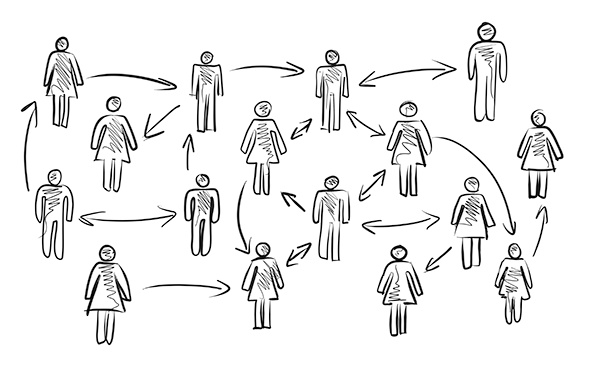
(b) directed network

Figure 2: The interaction network can be undirected or directed. In an undirected graph relationships is assumed to be symmetric and bidirectional. In opinion dynamics an arrow from Alice to Bob means Alice puts some weights on Bob’s opinion, i.e. she listens to her.

Time

We can model time as continuous (Fig. 3(b)), but this is usually not the choice. Therefore, in each of the models we review in this paper, time is discrete: $t=0,1,2,\dots$ (Fig. 3(a)).

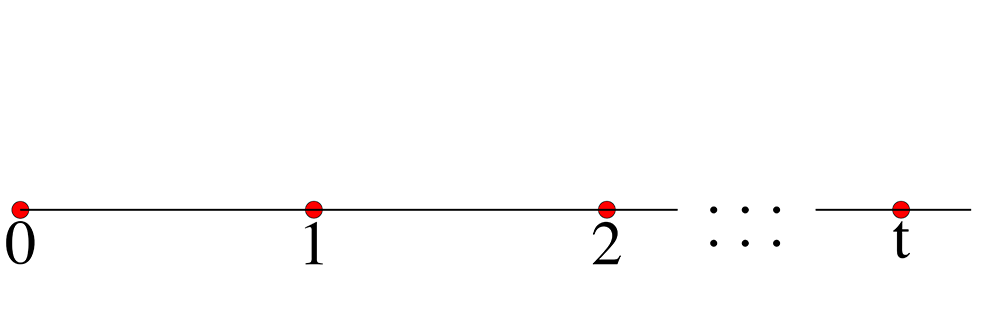
(a) discrete time steps

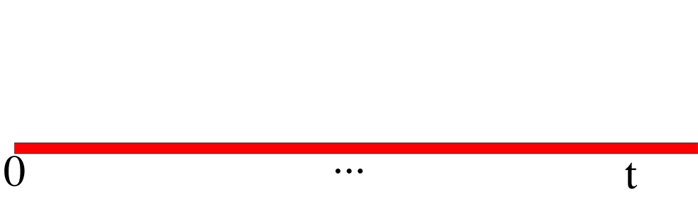
(b) continuous time

Figure 3: The time in the opinion dynamics can be discrete, e.g. the DeGroot model [2], or continuous e.g. the Altafini model [4].

1.2 Outline of the Paper

We begin by providing some definitions (Sec. 2.1) that are needed to either establish the models or present of the results. Then we briefly present the classical models of opinion dynamics (Sec. 2.2) for readers who are new to the field, and to refresh the memories of readers who have some knowledge of them; these classical models will be the foundations for the extensions presented later in the paper.

In Sec. 3, we study the simple DeGroot model and its variants which permits the use of advanced linear algebra insights and tools. In this model, the opinions of all participants are usually updated simultaneously. In Sec. 4, we consider the bounded confidence models. Then, in Sec. 5, models that include repulsive forces are discussed. Other works that we did not cover in detail will also be touched upon in this section and we will make suggestion for future research directions.

The paper is organized based on the DeGroot model and its extensions and the bounded confidence models and their extensions. Moreover, not all concepts are applied to all the models. For example, a repulsive behavior has not been applied to the HK model. Therefore, Sec. 3 includes a subsection devoted to repulsive forces but the Sec. 4 does not.

Hence, the organization of the paper cannot be solely based on models or based on concepts. The final section includes novel models and some of influential works that did not fit into the framework of well-known models.

1.3 Note on terminology

Before diving into the definitions we would like to mention that there is no convergence on terminology in the literature. Many of the model names are text dependent, i.e. different models may be known by the same name in different articles. For example, most authors by “bounded confidence model” refer to the DW model [5], however, any model with a confidence radius beyond which agents ignore each other can be referred to as a bounded confidence model. The Hegselmann-Krause version of the bounded confidence model is given by:

$$o_{i}^{(t+1)}=\frac{1}{|N_{i}^{(t)}|}\sum_{j\in N_{i}^{(t)}}o_{j}^{(t)}$$ (1)

where $N_{i}^{(t)}=\{j||o_{i}^{(t)}-o_{j}^{(t)}|\leq r_{i}\}$ is the set of agents whose opinions fall in the confidence interval of agent $i$ at time $t$, i.e. hold close-enough opinions. A general framework is established in Hegselmann-Krause’s work and then different directions are studied, all of which are referred to as HK model in different works. Proskurnikov[6] refers to the model given by Eq. (1) as the HK model, and not bounded confidence model. It is noteworthy that in the DW model the update rule is a function of the difference of opinions of the pair, however, in Eq. 1 the update is independent of differences.

In the equation above, agent $i$ weighs its own opinion and that of other nodes equally. Fu et al. [7] modifies it so that agent $i$ can weigh its own opinion freely. He uses the term “stubborn” for agents who never change their opinions; however, in other works stubbornness refers to agents who incorporate their “initial” opinion [8], partially, to their current opinion. Hence, a more accurate terminology could be the use of fully and partially stubborn. A fully stubborn agent can be considered as a node that spreads a fixed opinion, regardless of that of others - much like a source of propaganda intended to forcibly shift the opinion of a population.

2 Basic definitions, notation and classical models

In this section we define notations and concepts that will be used globally in this paper. Local variables that are applicable only in specific situations will be defined within the appropriate sections.

The purpose of this section is to avoid misunderstanding and introduce ideas and terminology from a variety of fields. We need the definitions to present the results. For example, Thm. 3.4 uses graph properties and Prop. 3.1 uses properties of the weight matrix to state relevant results. This section also clarifies confusing terminologies for first-time readers, e.g., consensus versus convergence. Moreover, there are terms about which the community of researchers is not yet in total agreement, for example leaders vs stubborn-agents. We will present all models with a unified terminology (see 2.1).

2.1 Definitions and Notations

Definition 2.1.

A graph $\mathcal{G}$ is an object consisting of two sets, $V$ and $E$, denoted by an ordered pair $\mathcal{G}=(V,E)$, where $V$ is a finite nonempty set where each of its members is called a vertex or node, and $E$ is a subset of $V\times V$ where each of its elements is called an edge. An edge connecting a given vertex to itself is called a loop. In a social network a vertex is an agent, such as a person. An edge represents the relationship between two agents.

Definition 2.2.

A path is a sequence of vertices from one node to the next using the edges.

For example the sequence $v_{0},v_{1},v_{2},\dots,v_{k-1},v_{k}$ is a path from $v_{0}$ to $v_{k}$, where $v_{i}$ and $v_{i+1}$, for $i\in\{0,1,2,\dots,k-1\}$, are connected by an edge.

Definition 2.3.

A connected graph is a graph in which there is a path between all pairs of nodes.

In this work we use the terms graph and network interchangeably; vertices represent agents; and edges represent connections between individual agents.

Definition 2.4.

The number of edges connected to a vertex is called the degree of that vertex.

Definition 2.5.

If the edges in the set $E$ given in the definition above are unordered, i.e. unoriented, such that $e=(x,y)=(y,x)=\{x,y\}$, then the graph is an undirected graph; otherwise, it is a directed graph or a digraph. In a directed graph, relationships can be unilateral, such as the relationship between a judge and the person being sentenced, or between a teacher and a student who will receive a grade.

Definition 2.6.

A weighted graph has a weight assigned to each edge.

The weights associated with edges in a graph can represent various factors such as geographical distance, the probability of interaction between the two agents related by a given edge, or the influence an agent has over another agent. For example, the weights assigned to edges are similar to powers assigned to relationships; for example, the power of a teacher over a student tends to be much greater than the power the student has over the teacher. The assignment and values of weights are dependent on the goals of the model.

Definition 2.7.

Two vertices $v_{i}$ and $v_{j}$ are said to be adjacent if there is an edge connecting them. This definition gives rise to the adjacency matrix $\mathbf{A}=\mathbf{A}(\mathcal{G})=(a_{ij})=(\mathbf{A}_{ij})$. In an unweighted graph

$$\mathbf{A}_{ij}=\begin{cases}1&\text{if $(v_{i},v_{j})\in E$,}\\ 0&\text{o.w.}\\ \end{cases}$$

In a directed graph we might have $a_{ij}\neq a_{ji}$. Some graphs are weighted such that the weight assigned to each edge represents the influence of each agent on the other. (The weights also could represent the probability or the frequency of interactions, or other variables.) In this case the adjacency matrix can also be referred to by weight matrix or influence matrix. In this paper we use the terms adjacency matrix or weight matrix or influence matrix interchangeably, and while each entry of the matrix will be denoted by $w_{ij}$ the matrix itself still will be denoted by $\mathbf{A}$.

$$\mathbf{A}_{ij}=\begin{cases}w_{ij}&\text{if $(v_{i},v_{j})\in E$,}\\ 0&\text{o.w.}\\ \end{cases}$$

For a weighted graph, the indicator of the influence matrix $\mathbf{A}$ is a matrix whose entries are 1 whenever $\mathbf{A}_{ij}>0$ and zero whenever $\mathbf{A}_{ij}=0$. We use $\mathbf{A}$ for both whenever it does not cause confusion.

Remark 2.1.

Similar to $\mathbf{A}(\mathcal{G})$, which is the adjacency matrix induced by graph $\mathcal{G}$, $\mathcal{G}(\mathbf{A})$ is a graph induced by $\mathbf{A}$.

Definition 2.8.

A full graph or a complete graph is a graph in which all nodes are adjacent to each other.

Definition 2.9.

The set of all possible (numerical) opinions, denoted by $\mathcal{O}$, is called the opinion space. Examples of opinion spaces are $\{0,1\}$ for binary opinions, $[0,1]$, $[-1,1]$, simplices in $\mathbb{R}$, etc.

Definition 2.10.

Define the indicator function by

$$\mathbbm{1_{\mathcal{A}}}(x)=\begin{cases}1&\text{if $x\in\mathcal{A}$,}\\ 0&\text{if $x\not\in\mathcal{A}$}\\ \end{cases}$$

for a given set $\mathcal{A}$.

Example 2.1.

Let $x=-0.2$ and $\mathcal{A}=[-1,1]$, then, since $x=-0.2\in[-1,1]=\mathcal{A}$ we have $\mathbbm{1_{\mathcal{A}}}(x)=1$. One can use the following notation as well: $\mathbbm{1}(x\in\mathcal{A})=1$.

Please note the same idea can be defined when $\mathcal{A}$ is a condition, and $\mathbbm{1_{\mathcal{A}}}(x)=1$ whenever the condition $\mathcal{A}$ is met.

Definition 2.11.

Opinions held by agents are defined as:

• The opinion of agent $i$ at time $t$ is $o_{i}^{(t)}$.

• Let $\mathbf{o}^{(t)}=[o_{1}^{(t)},o_{2}^{(t)},\cdots,o_{N}^{(t)}]$ be the vector of opinions of all agents; this is also referred to as a profile in some articles. $N$ will denote the population of the network.

• The set of neighbors of node $i$ is denoted by $N_{i}$ when including itself, and by $N_{\bar{i}}$ when excluding itself; this notation allows graphs to contain self-loops, and to use or exclude the opinion of agent $i$ in updates.

As mentioned before some of the terminology in the field is not standardized. For example, Dong et al. [9] defines a leader as an agent who is connected, directly or indirectly, to all other agents and Dietrich et al. [10] defines a leader as an agent who does not change its opinion whatsoever. Yet, the latter definition is used to describe a fully-stubborn agent in some other texts. We will use unified definitions for these cases.

Definition 2.12.

A connected-agent is an agent that is connected directly or indirectly to all other agents. We will denote it by CA. In the case of digraphs there is a path from all agents to the connected agent.

Definition 2.13.

A fully-stubborn agent is an agent that does not change its opinion at all. A partially-stubborn agent is an agent that incorporates its initial opinion in subsequent updates, but is open to change. Stubbornness is denoted by $1-d_{i}$, where $d_{i}$ is the measurement of susceptibility to influence. If $1-d_{i}=0$, then the agent $i$ is called non-stubborn; if $0<1-d_{i}<1$, then the agent is called partially-stubborn; and if $1-d_{i}=1$, then the agent is fully-stubborn.

Definition 2.14.

A fully-stubborn agent that is connected directly via an edge to all other agents is labeled as media.

The terms leader, fully-stubborn agent or media can be used in the contexts in which agents purposefully steer or manipulate other agents toward consensus or even more specifically toward a pre-determined opinion.

Definition 2.15.

Let $\mathbf{A}$ be a given matrix. The $t$-th power of the matrix is denoted by $\mathbf{A}^{t}=\underbrace{A\times A\times\cdots\times A}_{\text{t times}}$.

Definition 2.16.

For a dynamically changing adjacency matrix, the adjacency matrix at time $t$ is given by $\mathbf{A}^{(t)}$.

Definition 2.17.

The vector $\mathbf{e}_{k}$ is a vector with 1 in its $k^{th}$ position and zeros elsewhere.

Definition 2.18.

The consensus value is the opinion shared by all agents and is denoted by $o^{*}\in\mathcal{O}$.

Definition 2.19.

Convergence is defined as an equilibrium state, which may or may not be the consensus state. The equilibrium state is denoted by $\mathbf{O}^{*}$.

If the equilibrium state coincides with consensus, then all its elements are identical; $\mathbf{O}^{*}=\left[o^{*},o^{*},\dots,o^{*}\right]$.

Definition 2.20.

Polarization refers to existence of two distinct groups that are not necessarily at opposite extremes.

Definition 2.21.

A bounded confidence model is a model in which agents ignore other agents whose opinions are too far from their own and take into account the opinions of agents that are close enough to their own. The region within which an agent considers other opinions in is called the confidence interval of the agent. In Fig. 4 the blue intervals are confidence intervals of agents where other opinions can be considered during an interaction.

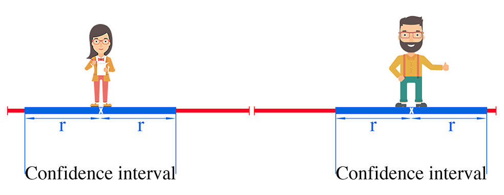
(a) homogeneous and symmetric

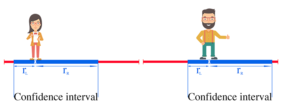
(b) homogeneous and asymmetric

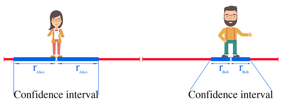
(c) heterogeneous and asymmetric

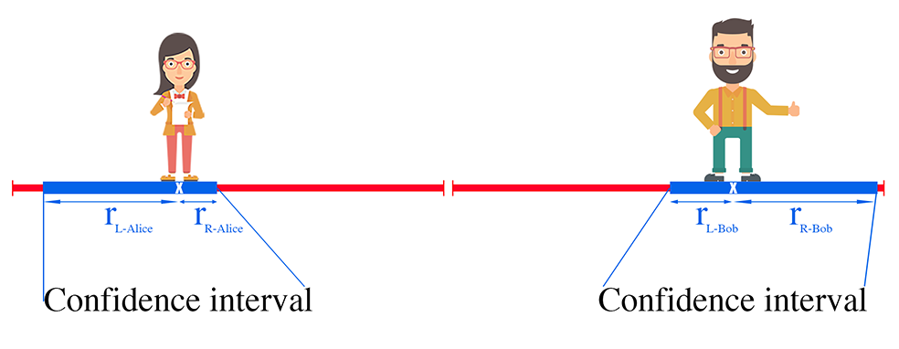
(d) heterogeneous and asymmetric

Figure 4: confidence interval types. In these figures the opinion space, e.g. $[0,1]$, is in red and the blue lines define the area where an interaction partner’s opinion can fall and be accepted by Alice or Bob. An agent’s opinion is shown by a white “X”. In 4(a) both agents have the same confidence interval, hence the system is homogeneous (in terms of the confidence interval, not the learning rate) and the intervals are symmetric. In 4(b) both agents have the same confidence interval, hence the system is homogeneous, but the intervals are asymmetric — agents are more accepting of opinions that are closer to 1, i.e. more than the agents’ current opinion. In figures 4(c) and 4(b) we see Bob’s and Alice’s intervals are different from each other, i.e. the system is heterogeneous. In the former case, the intervals are symmetric, while in the latter they are asymmetric.

If all agents have the same symmetric confidence interval, the interval’s radius is denoted by $r$. If the confidence levels differ for left and right, they are denoted by $r_{l}$ and $r_{r}$, respectively. Cases in which all agents enjoy identical confidence intervals are referred to as homogenous models. If each agent has its own confidence radius, it is denoted by $r_{i}$ in the case of symmetric confidence intervals. If the confidence levels are different for left and right, they are denoted by $r_{il}$ and $r_{ir}$, respectively; such models are referred to as heterogenous systems.

Note Homogeneous is used for two purposes: 1. to indicate that all agents share the same confidence interval, or 2. to indicate that they share the same learning rate, i.e. the same step size coefficient in updating an opinion due to an interaction. Likewise, heterogeneity can be used for two purposes. Note that in a given system, agents can be simultaneously homogeneous with respect to confidence interval and heterogeneous with respect to learning rate, and all other combinations of homogeneity/heterogeneity.

To refresh the memory of readers, we briefly list the well-known models that have been the foundation of opinion dynamics and other scientists’ works. Then we delve into the most recently published modifications of these models.

2.2 Classical models

1. The DeGroot[2] model, a simple averaging scheme that defines a linear system that can be analyzed by classical linear algebra, is given by

   $$\mathbf{o}^{(t)}=\mathbf{Ao}^{(t-1)}=\mathbf{A}^{2}\mathbf{o}^{(t-2)}=\cdots=\mathbf{A}^{t}\mathbf{o}^{(0)}$$ (DeGroot)

   where $\mathbf{A}$ is a row stochastic matrix of weights. In the original paper‚ stochastic indicated row stochastic and doubly stochastic referred to a matrix whose row sums and column sums each add up to 1. The matrix entries are the weights that a given agent puts on other agents’ opinions, i.e. the weights determine how much a given agent is influenced by any other agent. The updates in this model are synchronous. The stochasticity of the adjacency matrix means that the weights each agent puts on all of its friends/neighbors, including itself, add up to 1 or 100%. So, everything an agent learns is calculated exactly by the amount he trusts his friends and himself.

2. The Friedkin-Johnsen (FJ) model, which was introduced in 1990[11] and 1999[12], is given by (the FJ model is extension of the DeGroot model that includes stubborn agents):

   $$\mathbf{o}^{(t+1)}=\mathbf{D}\mathbf{Ao}^{(t)}+(\mathbf{I}-\mathbf{D})\mathbf{o}^{(0)}$$ (FJ)

   where $\mathbf{D}=diag([d_{1},d_{2},\dots,d_{N}])$ with entries that specify the susceptibility of individual agents to influence, i.e., $(1-d_{i})$ is the level of stubbornness of agent $i$, and $\mathbf{A}$ is a row stochastic matrix. In this model, agents are attached to their initial opinions, and are referred to as stubborn agents. If the adjacency matrix with entries that are influence weights is not symmetric then we can assume its associated graph is a digraph. Updates of the system are synchronous.

3. A well-known bounded confidence model is introduced by Deffuant and Weisbuch [5], commonly referred to as the DW model, is given by:

   $$\begin{cases}o_{i}^{(t+1)}=o_{i}^{(t)}+\mu\>.\>\mathbbm{1}_{[0,r]}(|d_{ji}^{(t)}|)\>.\>d_{ji}^{(t)}\\ o_{j}^{(t+1)}=o_{j}^{(t)}+\mu\>.\>\mathbbm{1}_{[0,r]}(|d_{ij}^{(t)}|)\>.\>d_{ij}^{(t)}\\ \end{cases}$$ (DW)

   in which at any given time the pair $i$ and $j$ are chosen randomly and $d_{ji}^{(t)}=o_{j}^{(t)}-o_{i}^{(t)}$. The parameter $\mu$ is called the learning parameter or the convergence parameter and usually is taken in the interval $(0,0.5]$ to avoid crossover. Please note that for the basic DW model,

   • The system is homogeneous in learning rate $\mu$.

   • The system is homogeneous in confidence radius $r$.

   • The system updates are pairwise.

   An example of a bounded-confidence model interaction in which each person has a different level of openness/closedness would be the following: Assume Bob and Alice participate in an interaction. If the opinion of Bob is close enough to the opinion of Alice, i.e., Bob’s opinion falls in the blue region in 4(b), then Alice learns from him and her opinion gets closer to that of Bob. But Bob is not very open-minded toward those whose opinions are far smaller than his own opinion, i.e., Alice’s opinion does not fall in the blue region on the left side of Bob in Fig. 4(b), therefore Bob will not learn and his opinion will remain unchanged.

4. The most general form of the Hegselmann-Krause [13] (HK) model is given by:

   $$\mathbf{o}^{(t+1)}=\mathbf{A}(t,\>\mathbf{o}^{(t)})\mathbf{o}^{(t)}$$ (HK)

   where $\mathbf{A}(t,\>\mathbf{o}^{(t)})$ is an arbitrary function of time and opinion. This is the HK model in its most complex and flexible form, which is too complicated to study without simplification: “In this generality, however, one cannot hope to get an answer, neither by mathematical analysis nor by computer simulations.” Because Eq. (HK) is too general to be suitable for direct analysis, Hegselmann inevitably studied simplifications of it. Please note that the set of models studied in Ref. [13], regardless of the direction they take are all referred to as the HK model in other research papers.

   Note that by fixing the matrix $\mathbf{A}(t,\mathbf{o}^{(t)})\mathrel{\mathop{\mathchar 58\relax}}=\mathbf{A}$ the Eq. (HK) collapses to DeGroot. Please also note that fixing the matrix takes away the bounded confidence idea and the dynamic changes dramatically in nature.

   Setting $\mathbf{A}(t,\mathbf{o}^{(t)})\mathrel{\mathop{\mathchar 58\relax}}=\mathbf{A}(\mathbf{o}^{(t)})$ where the adjacency matrix is only dependent on the current profile, following the bounded confidence rule, results in a synchronous bounded confidence model.

In Sec. 3 we study models that are based on DeGroot and FJ models , defined above, and in Sec. 4 bounded confidence model extensions is discussed. An important difference between DeGrootian and bounded confidence model is that the former is linear and latter is nonlinear and more complex.

3 DeGrootian models and their applications

The DeGroot model is the simplest method used for representing opinion dynamics. Such a simple scenario is traceable in time and opinion space, enabling researchers to produce analytical results. Over the years, different modifications of and additions to the DeGroot model have been used to investigate a variety of real human traits such as stubbornness (the study of which gave rise to the FJ model in 1990); since then, the FJ model has undergone further developments, and here we look at some of the newest results: the evolution of the social power of agents in the DeGroot and FJ models over a sequence of topics, the co-evolution of expressed and private opinions, the evolution of opinions given sequentially dependent topics, and the evolution of an agent’s susceptibility to influence.

3.1 Power evolution

In any society, whether it be a colony of ants, a pride of lions, or the US house of representatives, any given member will have power over some and will be submissive to others. As time passes and issue after issue is addressed by the society, the type of hierarchy governing the individual agents will become more distinguishable and distinct. Depending on the particulars of the society in question, an autocrat may arise or a democracy may develop. The phenomena of power evolution has been studied by researchers [14, 15, 8, 16] and we will devote following two subsections to this type of scenario.

3.1.1 Evolution of social power in the DeGroot model over a sequence of topics

Let us start this section with a proposition about the DeGroot model that may enlighten the motivation for the rest of the section.

Proposition 3.1.

[Ref. [17]] The DeGroot model will reach consensus if and only if there exists a power $t$ of the adjacency matrix for which $\mathbf{A}^{t}$ has a strictly positive column.

This proposition basically states that if there comes a time that everyone in the community listens to an agent (directly or indirectly), i.e., takes his opinion into account, then the community will come to consensus eventually.

Proposition 3.2.

[Ref. [2]] Let $\mathbf{A}$ be an adjacency matrix for which the DeGroot model reaches consensus. Then the final state of the system is $\mathbf{o}^{*}\mathrel{\mathop{\mathchar 58\relax}}=o^{*}\mathbf{1}$, where:

$$o^{*}=\langle\bm{\ell}_{\mathbf{A}},\mathbf{o}^{(0)}\rangle$$ (2)

and $\mathbf{1}_{N}=[1,1,\dots,1]^{T}\in\mathbb{R}^{N}$ is the vector of size $N$. $\bm{\ell_{A}^{\text{T}}}$ is the left eigenvector of $\mathbf{A}$ associated with 1, i.e., $\bm{\ell_{A}^{\text{T}}}\mathbf{A}=1\bm{\ell_{A}^{\text{T}}}$, constrained to $\langle\bm{1}_{N},\bm{\ell_{A}}\rangle=1$. Since the entries of $\bm{\ell_{A}^{\text{T}}}$ are non-negative, the $o^{*}$ is a convex combination of the initial opinions.

Jia et al. [15] introduced a very realistic scenario involving the evolution of social power in which individuals become aware of their power to influence and control others and the outcome of debate on each topic under negotiation in a sequence of topics.

Let $\mathbf{0}_{N}=[0,0,\ldots,0]^{T}$ be the vector of zeros with length $N$. Let the simplex $\Delta_{N}$ be the set of points in $\{\mathbf{x}\in\mathbb{R}^{N}\ |\mathbf{x}\geq 0,\langle\mathbf{1},\mathbf{x}\rangle=1\}$. A nonnegative matrix $\mathbf{M}$ is irreducible if its associated digraph is strongly connected. A nonnegative matrix $\mathbf{M}$ is reducible if its associated digraph is not strongly connected.

In the DeGroot model the weight matrix is static and does not change over time for the given topic under discussion. Here we consider a sequence of topics or subjects $s=0,1,2,\dots$ where each topic is represented by the DeGroot model, i.e., the weight matrix $\mathbf{A}$ does not change over time for a given topic, although it changes from topic to topic. The changes depend on the outcome of the previous topic, i.e., $\mathbf{A}(s+1)$ depends on the outcome of topic $s$:

$$\mathbf{o}^{(t+1)}(s)=\mathbf{A}(s)\mathbf{o}^{(t)}(s)$$ (3)

Just as in the DeGroot model, each weight/adjacency matrix is stochastic. The diagonal entries, $a_{ii}$, determine the degree of openness to change and the off-diagonal entries, $a_{ij}$, determine the degree to which agent $i$ is influenced by agent $j$. The off-diagonal entries can be decomposed and written as $a_{ij}=(1-a_{ii})c_{ij}$ where the $c_{ij}$ values are referred to as relative interpersonal weights. Define the matrix $\mathbf{C}\mathrel{\mathop{\mathchar 58\relax}}=[c_{ij}]$ with diagonal entries equal to zero. Then $\mathbf{C}$ is stochastic and we refer to it as the relative interaction matrix. Note that the self-weights $a_{ii}(s)$ are topic dependent, however the matrix $\mathbf{C}$ is static and does not depend on the topic.

We can write

$$\mathbf{A}(s)=diag([a_{11}(s),a_{22}(s),\dots,a_{NN}(s)])+(\mathbf{I}-diag([a_{11}(s),a_{22}(s),\dots,a_{NN}(s)]))\mathbf{C}$$ (4)

From now on we assume that matrix $\mathbf{C}$, which is stochastic with zero diagonals, is irreducible unless otherwise stated. Based on this assumption, the influence matrix $\mathbf{A}(s)$ has a unique left eigenvector $\bm{\ell_{A}}$ with non-negative entries, normalized so that $\langle\mathbf{1},\>\bm{\ell_{A}}\rangle=1$, and associated with eigenvalue $\lambda=1$, i.e., $\bm{\ell_{A}}\in\Delta_{N}$. For a large variety of the self-weight vectors $[a_{11},a_{22},\dots,a_{NN}]$, the eigenvector $\bm{\ell_{A}}$ satisfies $\lim_{t\to\infty}\mathbf{A}^{t}=\mathbf{1}[a_{11},a_{22},\dots,a_{NN}]$, which explains consensus in the DeGroot model: $\lim_{t\to\infty}\mathbf{o}^{(t)}=\langle\bm{\ell_{A}},\mathbf{o}^{(0)}\rangle\mathbf{1}$. Hence, the entries of the left eigenvector $\bm{\ell_{A}}$ determine the contribution of each individual to the final state of the system, that is, this eigenvector defines the agents’ power. This fact, also mentioned in Props. 3.1 and  3.2, motivates the definition of the evolution of social power for a sequence of topics:

$$[a_{11}(s+1),a_{22}(s+1),\dots,a_{NN}(s+1)]=\bm{\ell}_{\mathbf{A}}(s)$$ (5)

In other words, the self-weights for topic $s+1$ are equal to the agents’ power contributions to the final state of the system for topic $s$. This leads us to the definition of the DeGroot-Friedkin model.

Definition 3.1.

Let a group of $N$ agents discuss a sequence of topics $s\in\mathbb{Z}_{\geq 0}$ and the matrix $\mathbf{C}$ be the relative interaction matrix. The DeGroot-Friedkin model is given by

$$[a_{11}(s+1),a_{22}(s+1),\dots,a_{NN}(s+1)]=\bm{\ell_{A}}(s)$$ (6)

where $\bm{\ell_{A}}(s)\in\Delta_{N}$ is the dominant left eigenvector of the adjacency/weight matrix:

$$\mathbf{A}(s)=diag([a_{11}(s),a_{22}(s),\dots,a_{NN}(s)])-(\mathbf{I}-diag([a_{11}(s),a_{22}(s),\dots,a_{NN}(s)]))\mathbf{C}$$ (7)

The following proposition is a bridge that connects the DeGroot-Friedkin model to dynamical systems theory, enabling the application of this model to dynamical systems and the establishment of results such as proof of the existence and uniqueness of fixed points. Before introducing the proposition let us introduce $\bm{\ell_{C}}$ as the left eigenvector of the relative interaction matrix $\mathbf{C}$ that corresponds to the eigenvalue $1$ such that $\langle\mathbf{1}\>,\>\bm{\ell_{C}}\rangle=1$. The $i^{th}$ entry of $\bm{\ell_{C}}$ is called the eigenvalue centrality score of agent $i$.

Proposition 3.3.

Let $(\mathbf{1},\bm{\ell}_{\mathbf{C}})$ be the eigenpair of relative interaction $\mathbf{C}\in\mathbb{R}^{N\times N}$. The DeGroot-Friedkin model is equivalent to

$$diag([a_{11}(s+1),a_{22}(s+1),\dots,a_{NN}(s+1)])=F(diag([a_{11}(s),a_{22}(s),\dots,a_{NN}(s)]))$$

where $F\mathrel{\mathop{\mathchar 58\relax}}\Delta_{N}\rightarrow\Delta_{N}$ is a continuous map given by

$$F(x)=\begin{cases}\vspace{.2in}\mathbf{e}_{i}&\text{if $\mathbf{x}=\mathbf{e}_{i}$,}\\ \left(\frac{c_{1}}{1-x_{1}},\frac{c_{2}}{1-x_{2}},\dots,\frac{c_{N}}{1-x_{N}}\right)^{T}\big{/}\sum_{i=1}^{N}\frac{c_{i}}{1-x_{i}}&\text{o.w.}\\ \end{cases}$$ (8)

and where $c_{i}$ is the $i^{th}$ entry of the left eigenvector $\bm{\ell_{C}}$.

If the relative interaction matrix $\mathbf{C}$ is doubly stochastic, then the left eigenvector associated with eigenvalue $1$ is $\bm{\ell_{C}}=\mathbf{1}/N$ and Eq. 9 simplifies to

$$F(x)=\begin{cases}\vspace{.2in}\mathbf{e}_{i}&\text{if $\mathbf{x=e}_{i}$,}\\ \left(\frac{1}{1-x_{1}},\frac{1}{1-x_{2}},\dots,\frac{1}{1-x_{N}}\right)^{T}\big{/}\sum_{i=1}^{N}\frac{1}{1-x_{i}}&\text{o.w.}\\ \end{cases}$$ (9)

Proposition 3.4.

If the relative interaction matrix is doubly stochastic, then the following two properties hold true:

1. The equilibrium points of the dynamical system given by $F$ are $\{\mathbf{1}/N,\>\mathbf{e_{1},\>e_{2},\dots,\>e_{N}}\}$

2. For all initial conditions $\mathbf{x}(0)\in\Delta_{N}\backslash\{\>\mathbf{e_{1},\>e_{2},\dots,\>e_{N}}\}$ we have $\lim_{s\to\infty}\mathbf{x}(s)=\mathbf{1}/N$.

The second property in Prop. 3.4 indicates that the DeGroot model results in consensus with the final opinion being an average of the initial opinions, thereby indicating equal social ranking among agents.

The authors [15] presented conclusions and results (which are not included here) for interaction networks, including a star graph with propositions similar to those above. We close this subsection with the following theorem:

Theorem 3.1.

Let there be $N\geq 3$ nodes in an interaction network (that is not a star graph) with a relative interaction matrix $\mathbf{C}$. Let $\bm{\ell_{C}}$ be the left eigenvector of $\mathbf{C}$ associated with eigenvalue $1$. Then, for the dynamical system defined by

$$[a_{11}(s+1),a_{22}(s+1),\dots,a_{NN}(s+1)]=F([a_{11}(s),a_{22}(s),\dots,a_{NN}(s)])$$ (10)

we have the following:

1. The set of points of $F$ is $\{\mathbf{x^{*},e_{1},e_{2},\dots,e_{N}}\}$ where $\mathbf{x}^{*}$ lies in the interior region of $\Delta_{N}$ and the ordering of the entries in $x^{*}$ is the same as that in $\bm{\ell}_{\mathbf{C}}$.

2. For all initial conditions $\mathbf{x}^{(0)}\in\Delta_{N}\backslash\{\mathbf{\>e_{1},\>e_{2},\dots,\>e_{N}}\}$ we have:

   $$\lim_{s\to\infty}[a_{11}(s),a_{22}(s),\dots,a_{NN}(s)]=\mathbf{x}^{*}$$ (11)

According to Thm. 3.1, if the network does not establish an individual with total power as a consequence of its graph topology (i.e., the graph is not a star graph) or if in the initial system the social ranking of individuals is not set up so that one has power over all others, then the social ranking amongst agents will converge to an egalitarian state in which all individuals have the same power.

Later Ye et al. [18] showed that the convergence discussed above is exponentially fast. And they also studied the case of dynamic topology in which the matrix $\mathbf{C}$ changes along the sequence of topics, i.e. $\mathbf{C}(s)$ is a function of $s$, and show the conditions under which the same results hold true.

3.1.2 Evolution of social power in FJ model over sequence of topics

Let us now consider the idea of the evolution of power over the course of a sequence of topics in the FJ model studied in Ref. [8]. The FJ model is an extension of the DeGroot model in which each agent has a memory and is attached to its initial opinion at time $t=0$ and cannot completely let go of it. This model is given by Eq. FJ in section 2. To refresh the readers’ memory, we repeat:

$$\mathbf{o}^{(t+1)}=\mathbf{D}\mathbf{Ao}^{(t)}+(\mathbf{I}-\mathbf{D})\mathbf{o}^{(0)}$$ (12)

where $\mathbf{D}=diag([d_{1},d_{2},\dots,d_{N}])$ with entries that are individuals’ susceptibility to  influence, i.e., $(1-d_{i})$ is the level of stubbornness of agent $i$. Moreover, since in this subsection we are applying the FJ model to a sequence of topics where each adjacency/weight matrix depends on the topic $s$ currently under discussion, we can rewrite the equation above as

$$\mathbf{o}^{(t+1)}(s)=\mathbf{D}\mathbf{A}(s)\mathbf{o}^{(t)}+(\mathbf{I}-\mathbf{D})\mathbf{o}^{(0)}(s)$$ (13)

As before, we can write the adjacency matrix as:

$$\mathbf{A}(s)\mathrel{\mathop{\mathchar 58\relax}}=diag([a_{11}(s),a_{22}(s),\dots,a_{NN}(s)])+(\mathbf{I}-diag([a_{11}(s),a_{22}(s),\dots,a_{NN}(s)]))\mathbf{C}$$ (14)

where $\mathbf{C}$ is a stochastic matrix with zeros on the diagonal; however, in this section we drop the irreducibility of $\mathbf{C}$. Let us define a few concepts followed by a definition of the FJ model modified to handle a sequence of topics.

Definition 3.2.

A directed graph is said to be strongly connected if every node is reachable from every other node, i.e. if there is a path between any node to any other node. A strongly connected component (SCC) of a graph $\mathcal{G}$ is a strongly connected subgraph of $\mathcal{G}$ and is maximal in the sense that no additional edge or vertex from $\mathcal{G}$ can be added to it without breaking the strong connectivity property.

Definition 3.3.

An SCC of graph $\mathcal{G}$ is called a sink SCC if there are no directed edges from it to the nodes outside of it.

To avoid repetition, we list a few assumptions here and refer to them later, as needed.

Assumption 3.1.

Every sink SCC of $\mathcal{G}(\mathbf{C})$ has at least one stubborn agent, and $d_{i}<1$ if for the self-weight vector we have $[a_{11}(0),a_{22}(0),\dots,a_{NN}(0)]=\mathbf{e}_{i}$.

Assumption 3.2.

$\forall i\>d_{i}<1$, $\exists j,\>s.t.\>d_{j}>0$.

Now we are ready to define the FJ model for a sequence of topics.

Definition 3.4.

Let $s=0,1,2,\dots$ be a sequence of topics, and assume Asm. 3.1 holds. Let $\mathbf{C}$ be the relative influence matrix, and let $\mathbf{D}=diag([d_{1},d_{2},\dots,d_{N}])$ be the susceptibility matrix. Then the FJ model for a sequence of topics (FJS) is given by:

$$[a_{11}(s+1),a_{22}(s+1),\dots,a_{NN}(s+1)]^{T}=(\mathbf{I}-\mathbf{D})(\mathbf{I}-\mathbf{A}^{T}(s)\mathbf{D})^{-1}\frac{\mathbf{1}}{N}$$ (15)

where the adjacency matrix, $\mathbf{A}(s)$, is given by Eq. 14.

Derivation of Eq. (15): By Eq. (12) we have

$$\begin{array}[]{lllllll}\mathbf{o}^{(t+1)}&=&\mathbf{DA}{\color[rgb]{0,0.88,0}{\mathbf{o}^{(t)}}}+(\mathbf{I-D})\mathbf{o}^{(0)}\\ &=&\mathbf{DA}\left[{\color[rgb]{0,0.88,0}{\mathbf{DA}\mathbf{o}^{(t-1)}+(\mathbf{I-D})\mathbf{o}^{(0)}}}\right]+(\mathbf{I-D})\mathbf{o}^{(0)}\\ &=&(\mathbf{DA})^{2}\mathbf{o}^{(t-1)}+\mathbf{DA}\mathbf{(I-D)}+(\mathbf{I-D})\mathbf{o}^{(0)}\\ &=&(\mathbf{DA})^{2}{\color[rgb]{0,1,1}{\mathbf{o}^{(t-1)}}}+\left[\mathbf{DA}+\mathbf{I}\right](\mathbf{I-D})\mathbf{o}^{(0)}\\ &=&(\mathbf{DA})^{2}\left[{\color[rgb]{0,1,1}{\mathbf{DA}\mathbf{o}^{(t-2)}+(\mathbf{I-D})\mathbf{o}^{(0)}}}\right]+\left[\mathbf{DA}+\mathbf{I}\right](\mathbf{I-D})\mathbf{o}^{(0)}\\ &=&(\mathbf{DA})^{3}\mathbf{o}^{(t-2)}+\left[(\mathbf{DA})^{2}+(\mathbf{DA})+\mathbf{I}\right](\mathbf{I-D})\mathbf{o}^{(0)}\\ &\vdots&\\ &=&(\mathbf{DA})^{t+1}\mathbf{o}^{(0)}+\left[(\mathbf{DA})^{t}+(\mathbf{DA})^{t-1}+\cdots+(\mathbf{DA})^{1}+\mathbf{I}\right](\mathbf{I-D})\mathbf{o}^{(0)}\end{array}$$ (16)

Therefore, since $\mathbf{DA}$ is strictly sub-stochastic, we have $\lim_{t\to\infty}(\mathbf{DA})^{t+1}=\mathbf{0}$ and

$$\lim_{t\to\infty}\left[(\mathbf{DA})^{t}+(\mathbf{DA})^{t-1}+\cdots+(\mathbf{DA})^{1}+\mathbf{I}\right]=\mathbf{(I-DA)}^{-1}$$ (17)

consequently,

$$\lim_{t\to\infty}\mathbf{o}^{(t+1)}=\mathbf{(I-DA)}^{-1}(\mathbf{I-D})\mathbf{o}^{(0)}$$ (18)

Assumption 3.1 implies that the system comes to consensus for each topic:

$$\lim_{t\to\infty}\mathbf{o}^{(t)}=(\mathbf{I}-\mathbf{D}\mathbf{A}(s))^{-1}(\mathbf{I}-\mathbf{D})\mathbf{o}^{(0)}$$ (19)

We refer to the matrix $(\mathbf{I}-\mathbf{D}\mathbf{A}(s))^{-1}(\mathbf{I}-\mathbf{D})$ as the final state matrix. The mean of the $i^{th}$ column of the final state matrix given by the $i^{th}$ element of $[(\mathbf{I}-\mathbf{D}\mathbf{A}(s))^{-1}(\mathbf{I}-\mathbf{D})]^{T}\frac{\mathbf{1}}{N}$ is the relative control agent $i$ has on the final opinions of other agents, i.e., the social power of agent $i$. The transpose of the final state matrix is stochastic, and it defines a continuous map from $\Delta_{N}$ to itself and hence has a fixed point in $\Delta_{N}$. Lets denote this map by $F(\mathbf{x})$:

$$F(\mathbf{x})=[(\mathbf{I}-\mathbf{D}\mathbf{A}(\mathbf{x}))^{-1}(\mathbf{I}-\mathbf{D})]^{T}\frac{\mathbf{1}}{N}=(\mathbf{I}-\mathbf{D})(\mathbf{I}-\mathbf{A}^{T}(\mathbf{x})\mathbf{D})^{-1}\frac{\mathbf{1}}{N}$$ (20)

Furthermore, this map indicates that the final state of the system for topic $s$, and hence the social power of agents with respect to topic $s+1$, is dependent on stubbornness, i.e., stubbornness is equivalent to social power.

Please note that in the definition above $\mathbf{x}\in\mathbb{R}^{N}$, where in Eq. 15, for simplicity and to avoid the introduction of new notation, we use $\mathbf{A}(s)$ to indicate that the adjacency matrix depends on each topic and can be written as Eq. 14, which is obtained by representing each element of $\mathbf{A}(s)$ as the product $\mathbf{A}_{ij}(s)\mathrel{\mathop{\mathchar 58\relax}}=(1-a_{ii}(s))\mathbf{C}_{ij}$, where the $a_{ii}(s)$ are the self-weights. So, $\mathbf{A}(s)$ emphasizes the dependence of the adjacency matrix on topic $s$, which in turn depends on the self-weights $[a_{11}(s),a_{22}(s),\dots,a_{NN}(s)]\in\mathbb{R}^{N}$.

Proposition 3.5.

For the map $F(\mathbf{x})$ given by Eq. 20 we have:

• F is continuous on $\Delta_{N}$ and is differentiable in its interior region.

• $\forall x\in\Delta_{N},\>F_{i}(\mathbf{x})\in[\frac{1-d_{i}}{N},\frac{1+\zeta}{N}]$ where $\zeta=\>\langle[d_{1},d_{2},...,d_{N}]^{T},\mathbf{1}\rangle-\>d_{min}$, and $d_{min}=\min\{d_{1},d_{2},...,d_{N}\}$.

Theorem 3.2.

Consider the dynamical system given by Eq. 15, and let $[a_{11}(0),a_{22}(0),\dots,a_{NN}(0)]\in\Delta_{N}$. Denote the set of fully stubborn agents, (i.e., $d_{i}=0$) with $\mathcal{V}_{f}$ and the set of partially stubborn agents (i.e., $d_{i}>0$) with $\mathcal{V}_{p}$. WLOG, assume $\mathcal{V}_{f}=\{1,2,\dots,r\}$ and $\mathcal{V}_{p}=\{r+1,r+2,\dots,N\}$. Then,

1. $\exists\mathbf{x}^{*}\in\Delta_{N}$ satisfies:

   1. $\forall i\in\mathcal{V}_{f},\mathbf{x}^{*}_{i}\geq\frac{1}{N}$, and, $\mathbf{x}^{*}_{i}=\frac{1}{N}\>\text{iff}\>\>\text{ for any }j\in\mathcal{V}_{p},\mathbf{C_{ji}}=0$

   2. $\forall i\in\mathcal{V}_{p},\>\mathbf{x}^{*}_{i}>\frac{1-d_{i}}{N},\text{and }\mathbf{x}^{*}_{i}<\frac{1}{N}\>\text{if}\>\>\mathbf{C_{ji}}=0\text{ for any }j\in\mathcal{V}_{p}$

   3. $\max_{i}\>\>\mathbf{x^{*}_{i}}<\frac{1}{N}(1+\langle{[d_{1},d_{2},\dots,d_{N}]^{T},1}\rangle)$

2. $\mathbf{x}^{*}$ is unique if $\max_{i}\>\>d_{i}<\frac{N}{N+2(1+\zeta)}$.

Theorem 3.2 shows that an autocracy is not a possible outcome for the system defined above, as constrained by the associated assumptions. Moreover, if two agents can influence a third one, then the more stubborn agent of the two will have more social power at the end.

Theorem 3.3.

Consider the dynamical system given by Eq. 15 for which Asm. 3.2 holds, and let $\zeta$ be defined as it was in Prop. 3.5. If $\max_{i}\>\>d_{i}<\frac{N}{N+2(1+\zeta)}$, then all trajectories of the dynamical system converge exponentially fast to the unique equilibrium point given in Thm. 3.2.

In Ref. [8] the author establishes a number of the properties for the system associated with a star graph. Moreover, the evolution of social power is considered for a single topic, as opposed to the evolution occurring over a sequence of topics with social power fixed for a given topic. The author shows that the two approaches have similar behavior and equivalent properties.

The idea of the evolution of social power over a sequence of topics has been empirically studied in Ref. [19]. In this model, for a strongly connected network with assumptions such as the ones outlined above, one dominant agent with maximal influence will typically emerge, with the rest of the agents having minimal influence. An example in which the above scenario does not happen is a fully connected graph with all individuals having the same level of influence at $t=0$. The findings of Ref. [19] involve mostly artificial experiments in which people are represented unnaturally as interacting simultaneously. However, one might consider a simultaneous interaction as equivalent to a pairwise interaction with a different influence matrix. For example, agent $i$ may be influenced by agent $j$ at some time $t$, and agent $j$ may have been influenced by agent $k$ at some earlier time. Hence, agent $i$ is influenced by agent $k$ indirectly, which one might consider a simultaneous interaction with agent $i$ allocating different influence weights to $j$ and $k$ in two pairwise and simultaneous interactions. It is the combination of influence weight and the frequency of interaction that matters, really.

3.2 Susceptibility evolution

A new line of thought in opinion dynamics is considered in Ref. [20], followed by Ref. [21]; while the idea upon which it is based‚ a dynamic susceptibility to persuasion‚ has a long(er) history in social psychology, the mathematical study of it in opinion dynamics is novel. Susceptibility to persuasion denotes the extent to which a given agent is willing to change its opinion. It is the opposite of stubbornness. In the FJ model:

$$\mathbf{o}^{(t+1)}=\mathbf{DAo}^{(t+1)}+\mathbf{(I-D)o}^{(0)}$$

Recall that $\mathbf{D}=diag([d_{1},d_{2},\cdots,d_{N}])$, where the level of stubbornness of agent $i$ is $1-d_{i}$; therefore, by definition, $d_{i}$ is agent $i$’s susceptibility to persuasion. Abebe et al. [20] built on the FJ model by studying the effects of manipulating the $d_{i}$’s. It seems reasonable to assume that the susceptibility to persuasion of the agents in a network can be influenced by different tools. Abebe ran simulations with the goal of determining how the opinion dynamic could be altered by changing the susceptibility to persuasion in order to maximize (or minimize) the sum of opinions at equilibrium; such optimization translates into the network being pushed toward one or the other of the two extreme points in opinion space, 1 or 0.

To follow Abebe’s work, take the FJ model and a simple undirected graph (where simple means there is no self-loop in the network, i.e., $\mathbf{A_{ii}}=0$, and $N_{i}=N_{\bar{i}}$). Let every agent put equal weight on all of its neighbors’ opinions, i.e., $\mathbf{A}_{ij}=1/|N_{\bar{i}}|,\>i\neq j$. Then the update rule for any given agent at time $t$ can be written as:

$$o_{i}^{(t+1)}=(1-d_{i})o_{i}^{(0)}+\frac{d_{i}}{|N_{\bar{i}}|}\sum_{j\in N_{\bar{i}}}o_{j}^{(t)}$$

The system is known to have an equilibrium solution given by:

$$\mathbf{o^{*}}=[\mathbf{I-DA}]^{-1}(\mathbf{I-D})\mathbf{o^{(0)}}$$

Therefore, the objective, maximization of the sum of opinions, can be written as a maximization of

$$f(\mathbf{o^{(0)}},[d_{1},d_{2},\cdots,d_{N}])=\langle\mathbf{1},\mathbf{o^{*}}\rangle$$ (21)

Abebe showed that this problem can be solved in polynomial time provided that the susceptibility to persuasion of all agents can be modified. However, if the number of agents is limited, the problem is NP-hard for which the author provides a greedy algorithm. Chan et al. [21] continued Abebe’s line of work and claimed that one of his findings is wrong. Chan also suggested an algorithm for use with large graphs. Although the aforementioned works examine the problem from an algorithmic point of view using computer science, the approach of changing the susceptibility to persuasion of the agents in a network existed in psychology before being utilized in the opinion dynamics community.

3.3 Sequentially dependent topics

Let us start this section with an example. Suppose you have built a machine that produces gears. The completed machine is making the gears, and now you want to use the gears to manufacture mechanical wrist watches. Now suppose that back at the beginning, before building the gear-making machine, you had not carefully considered the size of gears that would be necessary for watches, but you went ahead and built the machine anyway. Now, because you do not want to re-do everything, you keep the machine running, even though the gears it produces means the wrist watches have to be extra-large and clunky. This type of phenomena is known as path-dependency.

In reality, as in the FJ model, consensus may not occur over a single topic. However, in psychology and path-dependence theory it has been shown that consensus can occur over a sequence of topics that are dependent (or if a topic is arising repeatedly.) It has been shown that the connectivity of a social network is enhanced when a sequence of dependent topics is considered by a network. The connection between the influence network and the network of initial opinions for successive topics can illuminate why consensus can occur for topics later in the sequence. The quest for understanding was the motivation of Tian and Wang [22] when considering a sequence of successively dependent topics and the agents’ related opinions/decisions (like the example above) and studying the conditions under which a community can come to consensus or form clusters of opinions for a sequence of topics.

Moreover, in the FJ model stubborn agents are unwilling to change their opinions on a single topic. In path-dependence theory cognitive inertia is defined as people’s unwillingness to change their opinions over a sequence of chain-dependent topics. Hence, the FJ model for each topic is employed to study the opinion dynamics of sequentially dependent topics, where the stubbornness factor is equated with cognitive inertia. In a sequence of dependent topics an agent’s initial opinion for topic $s+1$ is a function of (or a trade-off between) the agent’s “cognitive inertia” and “being social”. In other words, each agent forms its initial opinion for topic $s+1$ by making a tradeoff between its initial opinion for topic $s$ and the initial opinions of others about topic $s+1$.

3.3.1 The model

Let us start by pointing out that Tian [22] uses the term interdependent in his work. However, we prefer the term sequential dependency because the terms interrelated, interdependent and coupled topics have been used earlier, and we believe that sequential dependency or perhaps chain-dependency are more accurately descriptive for this scenario; Parsegov et al. [23] discussed and defined topics that are interrelated or interdependent by: “Dealing with opinions on interdependent topics, the opinions being formed on one topic are influenced by the opinions held on some of the other topics, so that the topic-specific opinions are entangled. …Adjusting his/her position on one of the interdependent issues, an individual might have to adjust the positions on several related issues simultaneously in order to maintain the belief system’s consistency.” In addition, Noorazar [24] provided the following definition for coupling: “Change of opinion about topic $s_{k}$ as a result of change of opinion about topic $s_{\ell}$ is called coupling.”

In accordance with the definitions given above, if an agent discusses topic $s_{k}$ (with another agent), and as a result changes its opinion about topic $s_{k}$, that agent will also change its opinion about coupled topic $s_{\ell}$ as well, even though topic $s_{\ell}$ was not discussed during the interaction with the other agent. For example, Alice and Bob may talk only about education, but as a result, their opinions about gun control may also change even though they did not mention gun control at all during their discussion. In this case it is as though the agent is moving on a manifold or surface, such that if the agent moves in the $x$ direction, it must also move in the $y$ direction in order to stay on the manifold. For this reason, we use sequential dependency for the model proposed by Tian [22].

Suppose there is a sequence of topics $s=1,2,3,\cdots$, and we apply the FJ model to each topic:

$$\mathbf{o}^{(t+1)}(s)=\mathbf{DA}\mathbf{o}^{(t)}(s)+(\mathbf{I-D})\mathbf{o}^{(0)}(s)$$ (22)

As before, $\zeta_{i}=1-d_{i}$ will be the level of stubbornness, or cognitive inertia, and $d_{i}$ will be the susceptibility to influence. This is where the FJ model and the path-dependency theory, in which agents exhibit stubbornness over a sequence of dependent topics, collide. For this reason, “cognitive inertia”, $\zeta_{i}$, is taken to be the same as the level of stubbornness, $1-d_{i}$.

When presented with a topic $s+1$, agents will form an initial opinion about it; in order to do so, a given agent $i$ will minimize the following:

$$C_{i}(\mathbf{o})=\zeta_{i}({o}_{i}-o_{i}^{(0)}(s))+(1-\zeta_{i})\sum_{j=1}^{N}\mathbf{A}_{ij}({o}_{i}-{o}_{j})^{2}$$ (23)

The optimal solution, $x^{\dagger}$, satisfies

$$(\mathbf{I-DA})x^{\dagger}=\mathbf{(I-D)}\mathbf{o}^{(0)}(s)$$ (24)

We need the following definition to present the results of this section.

Definition 3.5.

In an SCC of digraph $\mathcal{G}$, if there exists a vertex that has parents belonging to other SCCs, we say that the in-degree of this SCC is nonzero; otherwise, we call it an independent strongly connected component (ISCC).

Proposition 3.6.

Eq. 24 has a unique solution if and only if there exists no non-stubborn ISCC in $\mathcal{G}(\mathbf{A})$.

Proposition 3.6 allows the use of the initial opinion for topic $s+1$ as the limiting opinion of topic $s$, i.e., $\mathbf{o}^{(0)}(s+1)=\lim_{t\to\infty}\mathbf{o}^{(t)}(s)$. For such a scenario/system, the authors [22] focused on the sequence of initial opinions of the topics and defined the consensus states of the system in terms of the initial opinions:

Definition 3.6.

The system given by

$$\begin{cases}\mathbf{o}^{(t+1)}(s)=\mathbf{DA}\mathbf{o}^{(t)}(s)+(\mathbf{I-D})\mathbf{o}^{(0)}(s)\\ \\ \mathbf{o}^{(0)}(s+1)=\lim_{t\to\infty}\mathbf{o}^{(t)}(s)\end{cases}$$ (25)

is said to reach consensus if: $\lim_{s\to\infty}{o}^{(0)}_{i}(s)=o^{*}\in\mathcal{O},\>\forall i$.

Next we consider a topological condition that ensures the system reaches consensus in the sense defined above,

Theorem 3.4.

Suppose there exists no non-stubborn ISCC, and there is no fully stubborn agent in the network. Then the system outlined above will reach consensus if and only if there exists a partially stubborn agent who has a directed path to any other partially stubborn agent.

This result, which hinges on the existence of an agent who can influence others directly or indirectly, is similar to what we have seen before in other systems. A corollary to the theorem above is that the system will form clusters if more than one ISCC is in the network and vice versa.

Another reasonable case, considered in Ref. [22], has the initial opinion of a given agent $i$ for topic $s+1$ be a weighted average of those agents whose limiting opinions on topic $s$ are close enough to that of agent $i$’s opinion on topic $s$. This is the bounded confidence adaptation of the system above in which the initial opinion of agent $i$ for topic $s+1$ is influenced only by those who hold similar opinions to him about topic $s$. Results similar to those from the system above also hold true for this adaptation of the bounded confidence dynamic.

3.4 Expressed vs. private opinions

In many situations the expressed opinion of an agent may be different from its candid belief, e.g., such as when a candidate is trying to capture voters’ attention. Such a discrepancy between the private and expressed opinions of people has been studied in psychological fields, for example by Asch [25] whose work has motivated numerous researchers [26, 27, 28] including Ye et al. [29]. The expressed opinion of an agent is the result of pressure to conform to the average expressed opinion of the group the agent belongs to (local public opinion), or to conform to the group norm. And the private opinions of the agents evolve under the influence of other agents, as a function of their expressed opinions. Of course agents have “resilience” in the face of social pressure and therefore their expressed opinions are different from their private opinions.

3.4.1 The model

Let the co-evolution of a given agent’s private ($o_{i}^{(t)}$) and expressed ($\tilde{o}_{i}^{(t)}$) opinions is given by

$$\begin{cases}\vspace{.1in}o_{i}^{(t+1)}=d_{i}\mathbf{A}_{ii}o_{i}^{(t)}+\left(d_{i}\sum_{j\neq i}\mathbf{A}_{ij}\tilde{o}_{j}^{(t)}\right)+(1-d_{i})o_{i}^{(0)}&\text{(based on FJ)}\\ \tilde{o}_{i}^{(t)}=\phi_{i}o_{i}^{(t)}+(1-\phi_{i})\sum_{j\in N_{i}}m_{ij}\tilde{o}_{j}^{(t-1)}\end{cases}$$ (26)

where we have the following:

• As before, $\mathbf{A}_{ij}$ is the weight agent $i$ puts on agent $j$’s opinion.

• $\mathbf{A}_{ii}$ is self-confidence (self-loops are allowed).

• $\mathbf{A}$ is row stochastic.

• Updates are synchronous, i.e., all agents update simultaneously.

• $(1-d_{i})$ is the level of stubbornness and $d_{i}$ is the susceptibility to influence.

• $m_{ij}>0\Leftrightarrow\mathbf{A}_{ij}>0$, where $\sum_{j\in N_{i}}m_{ij}=1$.

• $\phi_{i}\in[0,1]$ is agent $i$’s resilience to the pressure to conform.

• $\tilde{o}_{i}^{(0)}\mathrel{\mathop{\mathchar 58\relax}}=o_{i}^{(0)}$

For such a system, the conditions under which the opinions converge to their limits exponentially fast has been studied. The conditions under which expressed opinions and private opinions reach constant values (i.e., consensus) have been examined as well. Ye et al. also considered the interesting case in which the expressed opinions and private opinions of agents, at the limit, reach a state of persistent disagreement at equilibrium that is caused by “the presence of both stubbornness and pressure to conform.” The paper concluded with the application of such a system to Asch’s [25] experimental studies. Let us consider the details more carefully.

Define the vectors $\mathbf{\tilde{o}}^{(t)}=[\tilde{o}_{1}^{(t)},\tilde{o}_{2}^{(t)},\ldots,\tilde{o}_{N}^{(t)}]$, $\mathbf{o}^{(t)}=[o_{1}^{(t)},o_{2}^{(t)},\ldots,o_{N}^{(t)}]$. Re-write the influence matrix $\mathbf{A}=\mathbf{\tilde{A}}+\mathbf{\hat{A}}$ where $\mathbf{\hat{A}}$ is obtained by setting the diagonal of $\mathbf{A}$ to zero and $\mathbf{\tilde{A}}=diag([a_{11},a_{22},\ldots,a_{NN}])$. As in the FJ model $\mathbf{D}=diag([d_{1},\ldots,d_{N}])$, and let $\mathbf{\Phi}=diag([\phi_{2},\ldots,\phi_{N}])$. We can write Eq. 29 in matrix form:

$$\begin{bmatrix}\mathbf{o}^{(t+1)}\\ \mathbf{\tilde{o}}^{(t)}\end{bmatrix}=\mathbf{P}\begin{bmatrix}\mathbf{o}^{(t)}\\ \mathbf{\tilde{o}}^{(t-1)}\end{bmatrix}+\begin{bmatrix}(\mathbf{I}-\mathbf{D})\mathbf{o}^{(0)}\\ \mathbf{0}\end{bmatrix}$$ (27)

where $\mathbf{P}$ is a block matrix:

$$\mathbf{P}=\begin{bmatrix}\mathbf{P_{11}}&\mathbf{P_{12}}\\ \mathbf{P_{21}}&\mathbf{P_{22}}\end{bmatrix}=\begin{bmatrix}\mathbf{D(\tilde{A}+\hat{A}\Phi)}&\mathbf{D}\mathbf{\hat{A}}(\mathbf{I-\Phi})\mathbf{M}\\ \mathbf{\Phi}&(\mathbf{I}-\mathbf{\Phi})\mathbf{M}\end{bmatrix}$$ (28)

In Ref. [29], $\mathbf{\tilde{o}}^{(0)}$ is set to $\mathbf{\tilde{o}}^{(0)}\mathrel{\mathop{\mathchar 58\relax}}=\mathbf{o}^{(0)}$, though other choices are possible of course, and we get $\mathbf{o}^{(1)}=(\mathbf{DA+I-D})\mathbf{o}^{(0)}$.

Recall that a directed network is called strongly connected if there is a directed path between any pair of vertices.

Definition 3.7.

A cycle is a path with equal starting and ending vertices, and no other repeated vertices.

Definition 3.8.

An aperiodic graph is a graph in which the greatest common divisor of the lengths of all of its cycles is 1.

Assumption 3.3.

Suppose the influence/weight/adjacency matrix $\mathbf{A}$ is stochastic, $\mathcal{G}[\mathbf{A}]$ is aperiodic and $d_{i},\phi_{i}\in(0,1)$.

Theorem 3.5.

Suppose Asm. 3.3 holds and the agents’ (expressed and private) opinions evolve according to Eq. 29. Then the system will converge, exponentially fast, to its limit:

$$\begin{cases}\vspace{.1in}\lim_{t\to\infty}\mathbf{o}^{(t)}=\mathbf{o}^{*}=\mathbf{Ro}^{(0)}\\ \lim_{t\to\infty}\mathbf{\tilde{o}}^{(t)}=\mathbf{\tilde{o}}^{*}=\mathbf{So}^{*}\end{cases}$$ (29)

where $\mathbf{R=(I-(P_{11}+P_{12}S))}^{-1}\mathbf{(I-D)}$ and $\mathbf{S=(I-P_{22})}^{-1}\mathbf{P}_{21}.$

The theorem above shows that both expressed and private opinions at the limit depend on the initial private profile. The initial expressed opinion is forgotten. Hence, the choice of initial expressed profile will change the trajectory while reaching the limit, but not the final state. The matrices $\mathbf{R}$ and $\mathbf{S}$ are positive and stochastic, which means the final expressed and private profiles are convex combinations of the initial private profile.

Proposition 3.7.

Suppose $\mathbf{A}$ is stochastic and the network given by it is strongly connected and aperiodic. Also assume $\phi_{i}\in(0,1)$ and there is no stubborn agent in the network ($d_{i}=1$). Then the system given by 27 converges exponentially fast to a consensus value shared by both private and expressed opinions: $\lim_{t\to\infty}\mathbf{o}^{(t)}=\lim_{t\to\infty}\mathbf{\tilde{o}}^{(t)}=o^{*}\mathbf{1}$ where $o^{*}\in\mathcal{O}=\mathbb{R}$.

Let us examine the conditions that determine whether a discrepancy will exist between the private and expressed profiles. Let $\mathbf{v}_{min}\>(\mathbf{v}_{max})$ denote the minimum (maximum) of the vector $\mathbf{v}$.

Theorem 3.6.

Suppose the assumptions of Thm. 3.5 hold and the initial private profile is not at consensus, i.e. $\mathbf{o}^{(0)}\neq\alpha\mathbf{1}$, for some $\alpha\in\mathbb{R}$. Then we have:

$$\begin{cases}\vspace{.1in}\mathbf{o}^{(0)}_{max}>\mathbf{o}^{*}_{max}>\mathbf{\tilde{o}}^{(0)}_{max}\\ \mathbf{o}^{(0)}_{min}<\mathbf{o}^{*}_{min}<\mathbf{\tilde{o}}^{(0)}_{min}\end{cases}$$ (30)

and $\mathbf{\tilde{o}}^{*}_{min}\neq\mathbf{\tilde{o}}^{*}_{max}$. Furthermore, the set of initial profiles $\mathbf{o}^{(0)}$ for which exactly $m$ agents will have identical expressed and private opinions at the limit, i.e. $o^{(*)}_{k}=\tilde{o}^{(*)}_{k}$, lies in a subspace of $\mathbb{R}^{N}$ with dimension $n-m$.

Therefore, as long as stubborn individuals are in the network, a discrepancy will exist between expressed and private opinions. We have seen before that if every agent is maximally open, i.e. non-stubborn, then consensus will be reached. Now we can conclude that without pressure to conform ($\phi_{i}=1$), the agents’ expressed and private opinion would be the same. An interesting result of theorem 3.6 is that there is more agreement among the expressed opinions compared to the private opinions, at the limit.

3.5 Repulsive behavior in the DeGroot model

A recent model that incorporates the repulsion property is Ref. [30]. Dandekar et al. [31] modified the DeGroot model to account for bias among agents in the sense that agents will learn more from those whose opinions are closer to that of a particular agent. The modified equation is given by:

$$o_{i}^{(t+1)}=\frac{w_{ii}o_{i}^{(t)}+(o_{i}^{(t)})^{b_{i}}}{w_{ii}+(o_{i}^{(t)})^{b_{i}}\sum_{j\in N_{\bar{i}}}w_{ij}o_{j}^{(t)}+(1-o_{i}^{(t)})^{b_{i}}(\sum_{j\in N_{\bar{i}}}w_{ij}-\sum_{j\in N_{\bar{i}}}w_{ij}o_{j}^{(t)})}$$ (31)

where $o_{i}$ is the level of support for opinion 1, $1-o_{i}$ is (consequently) the level of support for opinion 0, and $b_{i}\geq 0$ is the bias parameter. Hence, $(o_{i}^{(t)})^{b_{i}}$ is the weight given to neighbors supporting opinion 1 and $(1-o_{i}^{(t)})^{b_{i}}$ is the weight given to neighbors supporting opinion 0.

Dandekar’s work motivated Chen et al. [30] to devise a model that supported both bias and repulsion, or “backfire”. In Chen’s model the opinion space is $\mathcal{O}=[-1,1]$, and the opinions products are used to assign dynamical weights to the edges, as opposed to static ones. The opinion space is set to include negative as well as positive opinions, so that products of opinions could be either positive (for attraction) or negative (for repulsion). The weights on the $e_{ij}$ edge at any given time is given by $w_{ij}^{(t)}=1+\beta_{i}o_{i}^{(t)}o_{j}^{(t)}$. The larger the value of parameter $\beta_{i}>0$ becomes, the greater the strength of both the bias and repulsion. The update rule is given by:

$$o_{i}^{(t)}=\begin{cases}\vspace{.2in}\frac{w_{ii}o_{i}^{(t)}+\sum_{j\in N_{\bar{i}}}w_{ij}^{(t)}o_{j}^{(t)}}{w_{ii}+\sum_{j\in N_{\bar{i}}}w_{ij}^{(t)}}&\text{, }w_{ii}+\sum_{j\in N_{\bar{i}}}w_{ij}^{(t)}>0\\ sgn(o_{i}^{(t)})&\text{o.w.}\\ \end{cases}$$ (32)

For $\beta_{i}\neq 0$, there are two cases:

• $w_{ij}<0$: In this case repulsion occurs: $\beta_{i}o_{i}^{(t)}o_{j}^{(t)}<-1$, where $o_{i}^{(t)}o_{j}^{(t)}<0$, i.e., agents hold opinions with opposing signs in $\mathcal{O}=[-1,1]$.

• If $w_{ij}>0$, then bias assimilation occurs.

  1. $\beta_{i}o_{i}^{(t)}o_{j}^{(t)}>0$: Both agents have either positive or negative opinions. In this case, agent $i$ takes agent $j$’s opinion more seriously if the level of agreement is high between the two.

  2. $-1<\beta_{i}o_{i}^{(t)}o_{j}^{(t)}<0$: opinions are opposed, but not too strongly. In this case agent $i$ assimilates the opinion of agent $j$, but to a lesser extent.

  If the update rule stated by Eq. (32) violates the boundaries of opinion space, it is clamped.

Consider two agents $i$ and $j$, where agent $j$ does not change its opinion. Then depending on the initial opinion of agent $i$ and the parameter $\beta_{i}$, $i$ can be attracted to $j$ or be repulsed by it so that $i$’s opinion ends up at either of the endpoints or it never changes its opinion, an unstable equilibrium similar to an unstable fixed point in dynamical systems. Let us take a look at a general case below.

Theorem 3.7.

Let $\mathcal{G}=(V,E)$ be any connected unweighted undirected graph. For all $i\in V$, $o_{i}^{(t)}\in(-1,0)\cup(0,1)$, $w_{ii}=1$, $\beta_{i}=\beta>0$. Let $|\mathbf{o}^{(t)}|$ be the vector whose elements are absolute values of the opinion vector and $\min(\mathbf{o}^{(t)})$ be the minimum entry of $\mathbf{o}^{(t)}$. Then,

• If $\beta>\frac{1}{[\min(|\mathbf{o}^{(0)}|)]^{2}}$, then $\forall i\in V\mathrel{\mathop{\mathchar 58\relax}}|o_{i}^{*}|=1$, i.e., polarization occurs.

• If $\beta<\frac{1}{[\max(|\mathbf{o}^{(0)}|)]^{2}}$, then there exists a unique $o^{*}\in[-\max(|\mathbf{o}^{(0)}|),\max(|\mathbf{o}^{(0)}|)]$ such that, $\forall i\mathrel{\mathop{\mathchar 58\relax}}|o_{i}^{*}|=o^{*}$, $o_{i}^{*}$ is the final opinion of agents as time goes to infinity.

Proposition 3.8.

Let $\mathcal{G}=(V,E)$. Let $V=V_{1}\cup V_{2}$ such that $V_{1}\cap V_{2}=\varnothing$ where all agents in $V_{1}$ hold the same initial opinion $o_{i}^{(0)}=o^{(0)}\in(0,1)$ and all agents in $V_{2}$ hold the same initial opinion $o_{i}^{(0)}=-o^{(0)}\in(-1,0)$, i.e., the opinions are opposite in sign, but equal in absolute value. Moreover, let $w_{ii}=1$ and $\beta_{i}=\beta>0$. Then:

• If $\beta>\frac{1}{(o^{(0)})^{2}}$, then, $\forall i\in V,|o_{i}^{*}|=1$.

• If $\beta=\frac{1}{(o^{(0)})^{2}}$, then the agents’ opinions do not change over time.

• If $\beta<\frac{1}{(o^{(0)})^{2}}$, then there exists a unique $o^{*}\in(-o^{(0)},o^{(0)})$ s.t. $o_{i}^{*}=o^{*}$.

3.6 Managing consensus in the DeGroot model

In the history of opinion dynamics to this day, researchers mostly have been hunting the conditions under which consensus occurs, e.g. Ref. [32]. One interesting part that has been missing up to this point is the question of how to prevent consensus, or perhaps how to manipulate the system to reach a desired final state, whether that state is consensus or not. Such questions are especially relevant in the era that we are now witnessing, which features the interference of various countries in other countries’ elections. Because of the importance of the dynamics of interference, researchers have recently begun to investigate such phenomena. The literature on interference is in its infancy, however, due to its importance we include a discussion on it here.

Dong et al. [9] studied how to manipulate a network to reach a desired consensus, and, if such manipulation is not possible, then how to manage the network to reach a given set of final opinions. We will start by presenting a definition and looking at the result.

Recall that an agent who can influence all other agents, directly or indirectly, is called a connected-agent (CA).

Definition 3.9.

If agent $i$ is not a connected-agent it is a follower.

Denote the set of connected-agents and the set of followers by $V^{CA}$ and $V^{follower}$, respectively. Moreover, let $\mathbf{A}$ be the matrix of influence weights that defines a directed graph.

Consider the DeGroot model in which each agent has a positive self-weight for its own opinion, $\mathbf{A}_{ii}\in(0,1)$, and is influenced by at least one agent other than itself, and distributes equal weight among all of its neighbors; in other words, if $N_{\bar{i}}$ is the set of neighbors of agent $i$ (other than itself) who can influence it, then each neighbor’s influence on agent $i$ is $\frac{1-\mathbf{A}_{ii}}{|N_{\bar{i}}|}$.

Theorem 3.8.

In the modified DeGroot model described above, agents will reach consensus if there exists at least one connected-agent.

Proposition 3.9.

If consensus is reached in this modified DeGroot model, the final opinion can be expressed as a combination of the initial opinions of the connected-agents. ( $o^{*}=\sum_{v_{i}\in V^{CA}}\lambda_{i}o_{i}^{(0)}$ where $\lambda_{i}\geq 0$.)

Theorem 3.8 makes it clear that it is sufficient to have at least one connected-agent, (i.e., an agent that is reachable by other agents), in the network to reach consensus, and the associated proposition suggests that it is possible to guide agents towards a particular opinion. The goal is then to add the minimal number of edges to the network to make the set of connected-agents nonempty. To achieve this goal, create a new graph $\hat{\mathcal{G}}=(V,\hat{E})$, obtained from ${\mathcal{G}}=(V,{E})$, where $E\subset\hat{E}$ such that $V^{CA}\neq\varnothing$.

$$\begin{cases}\vspace{.2in}\displaystyle{\operatorname*{minimize}_{\hat{E}}(|\hat{E}|-|E|)}\\ \text{subject to }E\subset\hat{E}\\ \hskip 57.81621ptV^{CA}\neq\varnothing\\ \end{cases}$$ (33)

This optimization problem can be solved in two steps:

1. Form a partition $M$ of the network into subnetworks with the following properties:

   • Each subgraph has at least one connected-agent.

   • The union of any pair of subgraphs has no connected-agent.

2. Add the minimum number of edges among the subgraphs in the partition to form $\mathcal{\hat{G}}$ (see Alg. 1).

Input : Graph $\mathcal{G}$ and its partition $M$

Output : A new graph $\mathcal{\hat{G}}$ with connected-agents.

1

2Let $\hat{E}=E$ and $\mathcal{G}^{(i)}(V^{(i)},E^{(i)})\in M$ be any subgraph, let $\mathcal{G}^{*}(V^{*},E^{*})=\mathcal{G}^{(i)}(V^{(i)},E^{(i)})$ and $N=M\backslash\mathcal{G}^{(i)}$

3

4while $N\neq\varnothing$  do

5      

6      let $\mathcal{G}^{(\tau)}(V^{(\tau)},E^{(\tau)})$ be any subgraph in $N$

7      

8      let $E^{add}=\{(v_{k},v_{l})|v_{k}\in V_{\mathcal{G}^{\tau}}^{\text{CA}},v_{l}\in V^{*}\}\cup\{(v_{m},v_{n})|v_{m}\in V_{\mathcal{G}^{*}}^{\text{CA}},v_{n}\in V^{\tau}\}$

9       let $e$ be any edge in $E^{\text{add}}$ and $\hat{E}=\hat{E}\cup\{e\}$ (update $\mathcal{G^{*}}(V^{*},E^{*})$ as follows)

10       $V^{*}=V^{(\tau)}\cup V*$

11       $E^{*}=E^{(\tau)}\cup E*\cup\{e\}$

12       $N=N/\mathcal{G^{(\tau)}}$

13 end while

14

return $\mathcal{\hat{G}}$

Algorithm 1 Adding Edges

Theorem 3.9.

The $\mathcal{\hat{G}}(\hat{V},\hat{E})$ obtained via Alg. 1 is the optimal solution to the optimization problem given by Eq. 33 and $|\hat{E}|-|E|=|M|-1$, where $M$ is the partitioning of $\mathcal{G}$.

The paper [9] also proposed a network modification that consisted of adding edges so that the final state lies within a target interval $o^{*}\in[o^{*}_{l},o^{*}_{r}]$. Perhaps future work will examine how to prevent a community from reaching consensus, such as what occurred in the most recent American presidential election.

3.7 A general stabilization condition

Recall that in the DeGroot [2] model each agent trusts the other agents by a fixed amount, and consequently the adjacency matrix $\mathbf{A}$ is fixed.

Lorenz [33] defined a model with an evolving weight (adjacency) matrix in which the entries (i.e., the level at which agents trust others) are a function of both time and current profile.

Fixing the weight matrix of Lorenz’s model will result in the DeGroot model. One can also define the weight matrix in Lorenz’s model so that the model collapses to a bounded-confidence model. As such, we use his work as a stepping stone to go from DeGrootian models to the bounded-confidence models in the next section.

The result of Ref. [33] is given below, after the introduction of some notation. Let $\mathbf{A}^{(t)}(\mathbf{o}^{(t)})$ be a stochastic adjacency weight matrix at time $t$ that is a function of both time and the opinion profile at time $t$, $o^{(t)}$. For simplicity we refer to this matrix as $\mathbf{A}^{(t)}$. Define the update rule by:

$$\mathbf{o}^{(t)}=\mathbf{A}^{(t-1)}\mathbf{o}^{(t-1)}=\mathbf{A}^{(t-1)}\mathbf{A}^{(t-2)}\mathbf{o}^{(t-2)}=\cdots=\mathbf{A}^{(t-1)}\mathbf{A}^{(t-2)}\cdots\mathbf{A}^{(0)}\mathbf{o}^{(0)}$$ (34)

Denote the last term in Eq. (34) by $\mathbf{A}(0,t)\mathrel{\mathop{\mathchar 58\relax}}=\mathbf{A}^{(t-1)}\mathbf{A}^{(t-2)}\mathbf{A}^{(t-3)}\cdots\mathbf{A}^{(0)}$ or more generally $\mathbf{A}(t_{0},t_{1})\mathrel{\mathop{\mathchar 58\relax}}=\mathbf{A}^{(t_{1}-1)}\mathbf{A}^{(t_{1}-2)}\mathbf{A}^{(t_{1}-3)}\cdots\mathbf{A}^{(t_{0})}$. Using this notation we can compactly write $\mathbf{o}^{(t)}=\mathbf{A}(0,t)\mathbf{o}^{(0)}$. The following theorem is provided by [33].

Theorem 3.10.

Let $A^{(t)}$ be the adjacency matrix of the Lorenz model defined above for a given network $\mathcal{G}=(V,E)$. If for any $t$ the matrix satisfies the following conditions:

• $\mathbf{A}_{ii}>0$

• $\mathbf{A}_{ij}>0\iff A_{ji}>0$

• $\exists\>\epsilon\>\forall\mathbf{A}_{ij}\neq 0,\>s.t.\>\mathbf{A}_{ij}>\epsilon$

then there exists a time $t_{0}$ and a pairwise disjoint subgroups of agents $S_{i}$ such that $\cup_{i=1}^{p}S_{i}=V$ and

$$\lim_{t\to\infty}\mathbf{A}(0,t)=diag(\mathbf{K}_{1},\mathbf{K}_{2},\ldots,\mathbf{K}_{p})\mathbf{A}(0,t_{0})$$ (35)

where $diag(\mathbf{K}_{1},\mathbf{K}_{2},\ldots,\mathbf{K}_{p})$ is a diagonal block matrix with blocks $\mathbf{K}_{i}\in\mathbb{R}^{|S_{i}|\times|S_{i}|}$. Moreover, each $\mathbf{K}_{i}$ has identical rows.

Theorem 3.10 states that if the adjacency matrix that assigns weights for the opinions of neighbors satisfies the three conditions, then for any initial set of opinions, the network will end up with separate clusters in which the agents of each subgroup come to consensus. In each of the block diagonal matrices each entry will be greater than zero, i.e., all agents within a subgroup will talk to any other agent in the group. This is one of the early interesting analytical results that motivated additional studies, including a number of the following modifications.

4 Bounded confidence models

One of the most famous types of model in the field is the so-called “bounded confidence”‚ model in which agents are influenced by those whose opinions‚ are close enough to their own. This modification is justified by the homophily observation and the tendency that “birds of a feather flock together.” In the model of Deffuant [5] (the DW model) the interactions are binary, for which Monte Carlo-driven results are in abundance. However, due to the model’s nonlinearity, theoretical results are scarce. We could mention Ref. [34] as an example of simulation-driven work in which for a homogenous (i.e., all agents share the same level of confidence) DW model it has been demonstrated that the confidence radius $0.5$ is the limit above which consensus occurs for a variety of network topologies. Lorenzo [35] has shown that if two types of agents‚ open-minded and closed-minded‚ with two different confidence radiuses are in the same network, then, counterintuitively, the final state will be consensus for confidence levels below the critical radius (of homogenous systems) of 0.5. According to simulations, the critical value between polarization and consensus is 0.27 for the DW model and 0.19 for the HK model.

Later, Hegselmann and Krause [13] established the model for synchronous updates for which theoretical results have emerged at a higher rate. Recently, the publication rate for analytical results for minor modifications to such models has increased.

4.1 Power evolution in a synchronous bounded confidence model

We start this section by studying power evolution in a bounded confidence model to have a consistent pattern with the last section. However, this study is a simulation based for which analytical results do not exist.

New approaches and concepts have been introduced in Ref. [36], with agents having the chance to change their connectivity in the digraph to maximize their influence. For example, when the opinion space is set to $\mathcal{O}=[-1,1]$, the influence of agent $i$ is defined as $I_{i}=|o_{i}-\bar{o}|$ where $\bar{o}$ is the average of all the agents’ opinions. $I_{i}=0$ indicates that the entire network is in total agreement with agent $i$, who has maximum influence; likewise, $I_{i}=2$ indicates total disagreement with agent $i$. In such a scenario, agent $i$’s goal would be to maximize its influence in the network. The dynamics of the model in Ref. [36] are given by the repetition of two alternating steps:

1. Update the opinions of agents synchronously

2. Rewire the network to maximize the influence of a particular agent

The first step is given by:

$$o_{i}^{(t+1)}=o_{i}^{(t)}+s\eta_{i}+\mu\sum_{j\in N_{i}}\mathbf{A}_{ij}d_{ji}$$ (36)

where $s$ is a parameter that strengthens or weakens the effect of random external noise $\eta_{i}$, and as before $N_{i}$ is the set of agent $j$s whose opinions fall within the confidence radius of agent $i$, that is, $|d_{ji}|=|o_{j}^{(t)}-o_{i}^{(t)}|<r$. The reason for incorporating $\mathbf{A}_{ij}$ above is that the network is not a complete graph, but a directed graph which may be incomplete. The second step involves rewiring, which is accomplished in the following way: $m$ agents are chosen randomly and each of them will consider rewiring (if all do decide to rewire, $m$ rewirings will take place). Then each agent (such as agent $i$) from among the $m$ agents, chooses an agent out of all agents which are not currently its neighbor (suppose agent $k$ is chosen by agent $i$ and they are not currently neighbors). Then agent $i$ predicts its influence (using Eq. 36) in the new topology where $i\rightarrow k$, without taking into account the external noise. If agent $i$’s influence has increased, then rewiring takes place. Simulations for the above scenario can be divided in two sub-categories: endogenous and exogenous. In the endogenous case, a large fraction of the agents in the network participate in the rewiring step that maximizes influence. In the exogenous case, external sources compete to maximize their influence on the network, while they themselves cannot be influenced by members of the network. Simulations can be run for different confidence radiuses $r$ and for various rewiring schemes. The main results are that: for small confidence radiuses, the population will be polarized into two sub-communities of comparable size; for medium-sized confidence radiuses, one of the two sub-communities will be significantly larger than the other; and for large confidence radiuses, consensus will be achievable. For more discussion of randomly changing topologies, please consult the references given in Ref. [36].

4.2 Convergence and convergence speed of heterogeneous (in confidence level) DW model

In the work of Ref. [37] a version of DW is considered in which each agent had its own confidence bound. From a probabilistic standpoint, it is shown that when the DW model is heterogeneous in confidence levels, the network will reach a final state in which any pair of agents either are in agreement, or the distance between them is greater than the confidence radius of the two. This means that if there are two communities, $C_{1}$ and $C_{2}$ in the network, then $C_{1}$ is at the consensus state, $C_{2}$ is at consensus state, and the distance between the two clusters, (or distance between the opinions of two group), is greater than the confidence radius of the most open-minded agents in the two communities.

4.2.1 The model

Let us start this section with a definition.

Definition 4.1.

The system almost surely comes to consensus if

$$p\left(\lim_{t\to\infty}o_{i}^{(t)}=o^{*}\right)=1,\>\forall i$$ (37)

where $o^{*}\in\mathcal{O}$. Similarly it will almost surely converge if $p\left(\lim_{t\to\infty}\mathbf{o}^{(t)}=\mathbf{o}^{*}\right)=1$.

Chen et al. [37] studied a heterogeneous (in confidence radius) DW model, i.e., each agent has its own confidence interval, and the learning rate is homogeneous.

Let $\mathcal{N}=\{(i,j)|\>i,j\in\{1,2,\cdots,N\},i<j\}$ be the set of pairs that is used to select a random pair to interact at any time. Then the update rule is defined by

$$\begin{cases}\vspace{.2in}o_{i}^{(t+1)}=o_{i}^{(t)}+\mu\>.\>\mathbbm{1}_{[0,r_{i}]}(|d_{ji}^{(t)}|)\>.\>d_{ji}^{(t)}\\ o_{j}^{(t+1)}=o_{j}^{(t)}+\mu\>.\>\mathbbm{1}_{[0,r_{j}]}(|d_{ij}^{(t)}|)\>.\>d_{ij}^{(t)}\\ \end{cases}$$ (38)

where $\mu$ is the learning rate and $d_{ji}^{(t)}=o_{j}^{(t)}-o_{i}^{(t)}$ is defined as before. In Chen et al.’s work $\mu=\frac{1}{2}$, and the introduction of $\mathbbm{1}_{[0,r_{i}]}(|d_{ji}^{(t)}|)$ follows Chen et al.’s notation and can be dropped with the understanding that this is in fact a bounded confidence model with updates that take place only if agents fall within each other’s confidence intervals. Order the agents so that the confidence radiuses of the agents are decreasing, i.e. $r_{1}\geq r_{2}\geq\cdots\geq r_{n}>0$. (We will make use of this ordering later.)

Theorem 4.1.

Consider the heterogeneous BC model whose update rule is given by Eq. 38. Assume each agent has a positive confidence radius and let the interactions be performed in a randomized pairwise fashion at any given time where all $N$ agents of the network $\mathcal{G}$ are fully connected. Then we have

$$\forall\mathbf{o}^{(0)}\in[0,1]^{N},\>\exists\>\mathbf{o}^{*}\in[0,1]^{N}\>\>\text{such that }$$

• $\lim_{t\to\infty}\mathbf{o}^{(t)}\xrightarrow{\text{almost surely}}\mathbf{o}^{*}$

• $\forall i\neq j,\>o^{*}_{i}=o_{j}^{*}$ or $\mathinner{\!\left\lvert o^{*}_{i}-o_{j}^{*}\right\rvert}>\max\{r_{i},r_{j}\}$

Corollary 4.1.

If the assumptions of Thm. 4.1 are met and one of the confidence bounds is greater than or equal to 1, then the network will almost surely reach consensus for any initial profile.

The convergence rate is established by:

Theorem 4.2.

Let the opinion dynamic system be given by Eq. 38 with positive confidence radiuses. Then for any initial state $\mathbf{o}^{(o)}\in[0,1]^{N}$ there exist $c\in\mathbb{R}$ s.t.

$$E\left[\sum_{i}^{N}(o_{i}^{(t)}-o_{i}^{*})^{2}\right]=O(exp(-ct))$$

where $E[.]$ denotes the expected value.

4.3 A more inclusive bounded confidence model

In the DW version of bounded confidence, if Alice and Bob are chosen at time $t$, they will interact if their opinions are close enough. In the HK model, Alice talks to all of her neighbors whose opinions are close enough. In the two bounded confidence models of Zhang and Hong [38] the situations are different. In the first version, at a given time Alice chooses several agents and updates her opinion using a subset of the chosen agents. The subset includes only the agents whose opinions are close enough to her own. In other words, the agents whose opinions are too far away are omitted from the update. The analytical results for this case also apply to the DW model since the DW model is a special case of the HK model. In the second version, Alice chooses several agents and computes a weighted average of their opinions, and if this value falls within her confidence level, then she uses it to update her opinion. The analytical result for the first scenario is that as time goes to infinity, any two agents are either in agreement or the distance between them is greater than the confidence radius $r$ which is shared among all agents. In the second scenario it is shown that as the confidence radius increases, consensus will occur more often.

Let us define the two scenarios more formally below.

4.3.1 The model

The first scenario is called Short-range Multi-choice DW (SMDW), in which agent $i$ has its own choice number $c_{i}$. At a given time $t$ agent $i$ chooses $c_{i}$ agents randomly, removes those whose opinions are too far from that of its own, and then updates its opinion by a weighted average of the opinions of the agents:

$$o_{i}^{(t+1)}=o_{i}^{(t)}+\mu_{i}\>.\sum_{j=1}^{c_{i}}\>w_{ij}\mathbbm{1}_{[0,r]}(|d_{ji}^{(t)}|)\>.\>d_{ji}^{(t)}$$ (39)

where $c_{i}$ is the number of agents that agent $i$ selects to learn from. The influence weights $0<w_{ij}\leq 1$ add up to 1 and they determine how much agent $i$ is influenced by each agent $j$’s opinion. Note that in Eq. 39 only those agents are taken into account whose opinions are close to that of agent $i$.

The second scenario, the Long-range Multi-choice (LMDW), is introduced below. Agent $i$ first chooses several agents to learn from. Then the overall weighted average of the opinions of the chosen agents are computed, and if this value falls within the confidence interval of agent $i$, then an update occurs; otherwise nothing happens. This arrangement allows agent $i$ to be influenced by some agents whose opinions would not have fallen within agent $i$’s confidence interval if they had participated in private interactions; in other words, opinions that fall outside of the confidence radius of agent $i$ can be influential now:

$$o_{i}^{(t+1)}=o_{i}^{(t)}+\mu_{i}\>.\>\mathbbm{1}_{[0,r]}(|y_{i}^{(t)}-o_{i}^{(t)}|)\>.\>(y_{i}^{(t)}-o_{i}^{(t)})$$ (40)

where $y_{i}=\sum_{j=1}^{c_{i}}w_{ij}o_{j}^{(t)}$. Let us examine the results and implications.

Theorem 4.3.

(SRMC Thm.) Let $\mathcal{G}$ be a fully connected graph with $N$ nodes. Let $r$ be the confidence radius for all agents whose interactions are governed by the Short-range Multi-choice Eq. 39; then, for any initial profile of the network given by $\mathbf{o}^{(0)}\in[0,1]^{N}$, one of the two following results will almost surely hold true for any pair of agents:

1. $\lim_{t\to\infty}d_{ij}^{(t)}=0$

2. $\lim_{t\to\infty}|d_{ij}^{(t)}|>r$

Theorem 4.4.

(LRMC Thm.) Let $\mathcal{G}$ be a fully connected graph with $N$ nodes. Let $r$ be the confidence radius for all agents whose interactions are governed by the Long-range Multi-choice Eq. 40. Furthermore, assume $c_{i}>1$, for all $i$. If

$$r\geq\max_{1\leq i\leq N}\min_{1\leq j\leq c_{i}}w_{ij}$$

then consensus can almost surely be reached.

Another paper that derives theoretical properties of opinion dynamics that are similar to those of Ref. [37] which is a minor modification of Ref. [38] is Ref. [39]. In Ref. [39], the LRMC Eq. 40 is modified so that all agents choose the same number of agents, $c$, to look up to and the weights $w_{ij}$ are all equal to $1/c$. The agents chosen to learn from can be chosen with replacement. Formally, the update rule is given as follows:

$$o_{i}^{(t+1)}=o_{i}^{(t)}+\mu\cdot\mathbbm{1}_{[0,r]}(|y_{i}^{(t)}|)\>y_{i}^{(t)}$$ (41)

where

• $y_{i}^{(t)}=\frac{{\sum_{j=1}^{c}o^{(t)}_{\mathcal{J}(i,j,t)}}}{c}-o_{i}^{(t)}$

• $\mathcal{J}(i,j,t)$ is the index of the agent selected by agent $i$ at its $j^{th}$ selection at time $t$.

• $c$ is a constant.

• The confidence radius $r$ and the learning rate $\mu$ both are in the interval $(0,1)$.

After the following definitions we will be able to represent the final result of Zhang et al.’s paper.

Definition 4.2.

Let $o_{[i]}^{(t)}$ be the opinion of the agent whose opinion at time $t$ is the $i^{th}$ largest opinion, i.e. the $i^{th}$ opinion when we order opinions: $o_{[1]}^{(t)}\leq o_{[2]}^{(t)}\leq\cdots\leq o_{[N]}^{(t)}$. Then we can define $D_{[i,i+1]}^{(t)}=o_{[i+1]}^{(t)}-o_{[i]}^{(t)}$ and the opinion range at time $t$ by $\Delta^{(t)}=o_{[N]}^{(t)}-o_{[1]}^{(t)}$.

The interesting result of this generalized model is obtained by stepping foot into the world of probability . The following theorem puts a lower and upper bound on the probability of consensus as a function of network population, $N$, confidence radius, $r$, and the selection parameter, $c$.

Theorem 4.5.

For the model defined by Eq. 41, let the population of the network be $N$, and the confidence radius $r$ be smaller than $\frac{1}{c}$, where $c$ is the selection parameter. Then the lower and upper bounds for the probability of convergence are given by:

$$N(cr)^{N-1}-(N-1)(cr)^{N}\leq p(\lim_{t\to\infty}\Delta^{(t)}=0)\leq\begin{cases}N!(cr)^{N-1}&\text{if $N\leq\lceil\frac{1}{cr}\rceil$,}\\ N!(cr)^{N-\lfloor\frac{1}{cr}\rfloor}&\text{o.w.}\\ \end{cases}$$ (42)

The convergence of $\Delta^{(t)}$ to zero is the convergence of the population to consensus, and if the assumptions outlined above are met, then we have $0<\ell\leq p(consensus)\leq u<1$, where $\ell$ and $u$ are the lower and upper bounds, respectively, defined in Thm. 4.5. Although computing the exact probability is impossible, a simple experiment is used to support the result.

4.4 A somewhat different bounded confidence model

In what we have seen before in BC models, any agent, like Alice, has only one confidence radius, Alice trusts everyone equally. However, in this section we have a DW model in which a given agent has more than one confidence radius. More precisely, Alice trusts her friends by different amounts (See Fig. 5). These confidence radiuses are assigned to edges like $e=(i,j)=(\text{Alice, Bob})$, i.e., relationships, via a random (Poisson) process. The confidence assigned to the edge, $e$ connecting Alice and Bob is denoted by $r_{e}=r_{\text{Alice-Bob}}$. The paper [40] that introduces this model starts by presenting analytical results for a 1-dimensional lattice (i.e., each agent only has two friends); this is followed by simulation results obtained from applications to ring and Barabási-Albert networks.

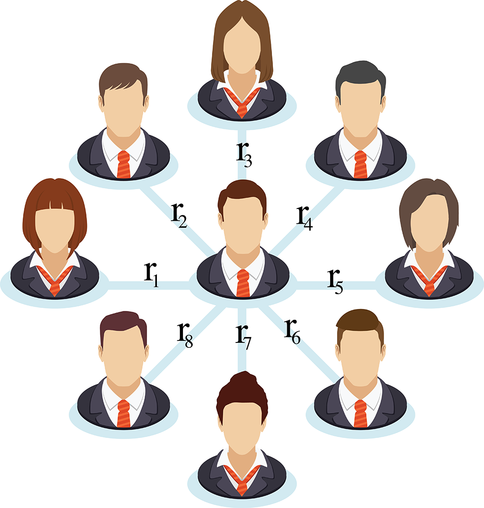
Figure 5: Edge dependent confidence intervals. In this case a given agent, like Alice, has more than one confidence interval—she has one per neighbor. She trusts different people differently.

The (analytical) result based on the 1D lattice is that $0.5$ is a critical value, in the sense that if the expected value of the confidence radiuses is below $0.5$, then, with a probability of one, any two adjacent agents are either at consensus or their opinions are far apart (by more than the confidence radius assigned to their relationship). And if the expected value of the confidence levels is more than $0.5$, then with probability one all agents will come to consensus with all agents having opinions of $0.5$. The simulations for ring and BA networks also suggest that $0.5$, as the expected value of the confidence radius, is a critical boundary between disordered and ordered phases of the system: the ordered phase of the network is in a consensus state, and the disordered phase lacks consensus.

The details are formally presented below:

4.4.1 The model

In this section we discuss a somewhat different bounded confidence model [40] that is based on the DW model. However, in this case

• The system is homogeneous in learning rate $\mu$.

• In this system confidence intervals are handled differently: every edge can have a different confidence interval.

• The system updates are pairwise.

In spite of this model using a 1-dimensional lattice network, whose agents sitting on the $\mathbb{Z}$ line, this modification of the DW model is interesting and will be discussed below. Originally Lanchier [41] proposed the model and geometrically proved that if the confidence radius is greater than 0.5 consensus will be achieved. Later Häggström [42] re-proved the conjecture, in a probabilistic framework, that was put forward using simulations. The aforementioned works are based on a homogenous network in which all agents share the same confidence level; however, in this section we focus on a heterogenous version [40] where the heterogeneity is implemented via a Poisson process.

Let $\mathbf{o}^{(0)}$ be the initial profile. For a given edge $e$, a random unit rate Poisson process is assigned that governs the interaction time as well as an i.i.d random variable $r_{e}$ whose values belong to $(0,1)$. Moreover, let the confidence radius $r$ be a random variable with the same distribution as $r_{e}$. Denote the opinion of a given agent, right before an interaction at time $t$, by $o_{i}^{(t_{-})}=\lim_{t\to t-}o_{i}^{(t)}$. Then the update rule is given as follows (similar to the discrete-time DW model):

$$\text{if}\>\>|o_{j}^{(t_{-})}-o_{i}^{(t_{-})}|<r_{e}\mathrel{\mathop{\mathchar 58\relax}}\begin{cases}o_{i}^{(t)}=o_{i}^{(t_{-})}+\mu(o_{j}^{(t_{-})}-o_{i}^{(t_{-})})\\ o_{j}^{(t)}=o_{j}^{(t_{-})}+\mu(o_{i}^{(t_{-})}-o_{j}^{(t_{-})})\\ \end{cases}$$ (43)

Please note that the confidence radius $r_{e}$ is assigned to an edge, i.e., each agent will have a different confidence radius for each neighbor. For a given edge $e_{ij}=\{i,j\}$ we denote $r_{i}=r_{e}$. The graph $\mathcal{G}$ is the set of integers $\mathbb{Z}$ unless otherwise stated.

Theorem 4.6.

Let an opinion dynamic be given by Eq. 43, with learning rate $\mu\in(0,0.5]$ and with $r_{i}$ assigned as random confidence radiuses for all $i\in\mathbb{Z}$, then:

• if $E[r]<0.5$ then $\forall i,\>p(\lim_{t\to\infty}|d_{i,i+1}^{(t)}|\in S)=1$, where $d_{i,i+1}=o_{i}^{(t)}-o_{i+1}^{(t)}$ and $S=\{0\}\cup[r_{u},1]$.

• if $E[r]>0.5$ then $\forall i,\>\lim_{t\to\infty}o_{i}^{(t)}=0.5$.

The above theorem states that neither the final profile of the network nor the critical confidence radius depends on the distribution of $r$ except for its expectation. Similar to the homogenous case, if $E[r]>0.5$ consensus is observed, and below that threshold fragmentation occurs, with the distance between neighboring communities connected via edge $e=e_{i,i+1}$ which is greater than $r_{e}$.

The extensive simulations presented in Ref. [40], show that these results hold for graphs that include the ring- and scale-free topology of Barabási with confidence radius parameters drawn from truncated normal distributions and from Beta distributions, each with a few parameters. These results agree with homogenous cases [34].

4.5 Noise in Bounded Confidence Models

Even though humans are capable of rational thought, they are still essentially emotional beings. A person may accept or reject the exact same idea depending on who is promoting it. In the previous sections of this paper the exchange of opinions among agents has taken place as though the agents are following a set of well-defined rules in a closed and isolated space, unaffected by external forces, or even by internal thoughts. However, such a scenario cannot accurately represent how opinions are exchanged in real life, where people are capable of changing their minds based on their own internal thought processes (without one-to-one interactions with others), or by reading (similar to a unilateral interaction in which one party does not change its mind). Moreover, in a single interaction the transmission of opinions is not absolutely perfect. Individuals usually find their own ways to be unique and distinct from the population as a whole. Such disintegrating actions can as a first approximation be represented by noise.

Hence, despite the lack of research on disintegrating forces or noise in social networks, especially with an analytical focus, we include such sections to emphasize its importance. The variation seen in opinion dynamics models is a testament to the difficulty of deriving specific results while using a given model; therefore, researchers modify the models of others to obtain desired results or to apply the models to scenarios that arise in their own fields. Therefore, not all modifications or papers presented in this section follow the same line of work. Let us start with analytical results for the case of noise added to the DW model.

4.5.1 The Noisy DW model

In order to eliminate the unrealistic sharp boundary between interacting and being indifferent in the bounded confidence of the DW, Grauwin and Jensen [43] introduced a probabilistic interaction schema to the DW model in which two agents interact with some probability that depends on their difference of opinion, interaction noise. This allows an agent the potential to interact with an agent whose opinion falls outside its confidence radius and to ignore an agent whose opinion falls within its confidence radius. A second type of noise is also considered by Grauwin and Jensen [43] that models death and birth of humans; at time $t$ an agent’s opinion randomly changes to a random number, they refer to it by turn over.

It has also been shown that dynamic and stable clusters can emerge in this model, as opposed to “frozen” clusters. Moreover, the authors claim that this noise is more natural than the one introduced by Mäs et al. [44] that is “specifically tailored to prevent consensus.”

It is shown that the introduction of interaction noise in the DW model (in the absence of turn over) causes consensus. The DW model with the additional ingredient of the turn over (in the absence of interaction noise) shows a different range of behaviors depending on the death/birth probability, changes in which cause a progression from an ordered phase to a disordered one. In the case that both interaction noise and turnover exist in the model, a phase transition happens for different combinations of the two parameters.

4.5.2 The model

Grauwin and Jensen [43] investigated the addition of noise to a specific DW model, namely, the one in which the learning rate is $0.5$. Said differently, an interaction means consensus between the two interacting agents. To be more precise, the update rule is the same as that of the standard DW model, however, the confidence rule is ignored some of the time (determined by a probability), which is the chosen method for implementing noise. In Grauwin and Jensen [43], two types of noise were added to the opinion dynamics:

• Type 1 Interaction noise: two randomly chosen agents at a given time step $t$ will interact with probability

  $$p_{int}=\left[1+exp(\frac{-1+|d_{ij}|/r}{\gamma})\right]^{-1}$$ (44)

  This noise acts as an integrating force, providing the opportunity for communities to come to consensus.

• Type 2 At any given time $t$, select a random agent and, with probability $\nu$, set its opinion to a random number within the opinion space $\mathcal{O}=[0,1]$. This noise acts as a disintegrating force, causing random behavior.

The probability of interaction, $p_{int}$, ensures that agents with opinion differences greater than the confidence radius $r$ have the chance to interact, which models rational choices in the real world. We do not just simply ignore all people who have opinions that differ from ours by a narrow margin. Note that a large $\gamma$ indicates that opinion difference is not very important.

The second type of noise, which is studied in the social sciences, is interesting, though to the best of our knowledge it has not been used before in opinion dynamics. The rationale for this type of noise is that some agents may die and new ones may be introduced to the system. Most current models consider the long-time behavior of agents as time goes to infinity, although individual human beings cannot exist in the system for that long, due to both death and the fact that we make and lose friends over the course of our lifetimes.

In Grauwin and Jensen [43], each community/cluster of agents is determined as follows: the agents are ordered by their opinions; if the difference between opinions of two neighboring agents is less than the confidence radius $r$, then they belong to the same group, chained together by the confidence radius, (in other words, if the difference between two consecutive agents’ opinions is more than $r$, then the number of clusters goes up by 1 and the two agents are the borders between the two clusters).

The results of adding these two types of noise to the model are described below:

• Let $\nu=0$; under this condition, we add only the probability of interaction between agents of two distinct communities separated by a distance greater than $r$; in other words, $\gamma>0$. In this case the system will end up in consensus because when two agents from different communities interact, their new opinions will be set to the average (since learning rate $\mu=0.5$) and this causes the communities to drift from their current states toward each other. The relationship between the parameters of the model and the time needed for the communities to merge into one is given in [43].

• Let $\gamma=0$, so that interactions are governed by the standard DW update rule, and let $\nu>0$. As expected, when $\nu$ is small, the system exhibits behavior similar to that of the DW model; likewise, when $\nu$ is large, chaos rules the system. In this type of scenario, one can define order parameters and apply statistical physics routines. The order parameter in [43] is given by

  $$\rho=S_{max}\>\left(1-3\frac{1}{{2\choose S_{max}}}\sum_{i,j\in g_{max}}|d_{ij}|\right)$$ (45)

  where $g_{max}$ is the largest cluster, and $S_{max}$ is the number of agents in $g_{max}$.

• Finally, it has been observed through the use of simulations that for a range of the pair of parameters $(\gamma,\nu)$, lasting communities will form.

4.5.3 The Noisy HK model

In this section we consider an extension of the HK model with noise added to it. In this section all agents share the same confidence radius $r$.

Su et al. [45] have shown that if the noise strength is smaller than $r/2$ then the noisy HK model will almost surely reach quasi-consensus. They also state that “HK dynamics is known to explain the divergence of opinions. However, our results reveal that the fragmentation behavior of the HK model fails to exhibit robustness against arbitrary weak random noise and that the mechanism of opinion divergence requires further study”. By means of simulation it has been shown that if the initial opinions of agents are identical and noise strength is larger than $r/2$, then agents will diverge at some point. If $r$ itself is too large, then consequently the noise will be too large as well, which causes fluctuations. Hence, the simulation that derived the aforementioned divergence in the presence of strong noise was conducted for $r=0.01$.

4.5.4 The model

Recall that the HK model is given by the following:

$$o_{i}^{(t+1)}=\frac{1}{|N_{i}^{(t)}|}\sum_{j\in N_{i}^{(t)}}o_{j}^{(t)}$$ (46)

Su et al. [45] added noise to this equation to obtain the following:

$$o_{i}^{(t+1)}=\xi_{i}^{(t)}+\frac{1}{|N_{i}^{(t)}|}\sum_{j\in N_{i}^{(t)}}o_{j}^{(t)}$$ (47)

Please note that $N_{i}^{(t)}$ is the set of agents whose opinions lie within the confidence interval of agent $i$ at time $t$, i.e., $|o_{i}^{(t)}-o_{j}^{(t)}|<r$ (here all individuals have the same symmetric confidence interval). The random noise $\xi_{i}^{(t)}$ can violate the boundaries of opinion space, in which case we apply the clamp function to it:

$$clamp(x)=\begin{cases}0&\text{if $x<0$,}\\ x&\text{if $0\leq x\leq 1$,}\\ 1&\text{if $x>1$.}\end{cases}$$ (48)

so, the update rule in the violating cases is:

$$o_{i}^{(t+1)}=clamp\left(\xi_{i}^{(t)}+\frac{1}{|N_{i}^{(t)}|}\sum_{j\in N_{i}^{(t)}}o_{j}^{(t)}\right)$$ (49)

We will now look at some definitions specific to this section and in the following subsections we will present experimental work related to noise as a disintegrating force.

Definition 4.3.

Let the diameter of opinions associated with the graph $\mathcal{G}$ at a given time $t$, and the limit diameter be given, respectively, by:

$$d_{\mathcal{G}}^{(t)}=\max_{i,j\in V}|o_{i}^{(t)}-o_{j}^{(t)}|\>\>\mathrm{and}\>\>d_{\mathcal{G}}=\lim_{t\to\infty}d_{\mathcal{G}}^{(t)}$$

Definition 4.4.

Define quasi-consensus (as before $r$ is the confidence radius):

• The system will reach a state of quasi-consensus if $d_{\mathcal{G}}<r$

• The system is said to almost surely reach quasi-consensus if $p(d_{\mathcal{G}}<r)=1$.

• The system will not reach a state of quasi-consensus if $p(d_{\mathcal{G}}<r)=0$.

• Let $t_{min}=\min\{t\>|\>d_{\mathcal{G}}^{(t^{\prime})}\leq r,\forall t^{\prime}\geq t\}$. If $p(t_{min}<\infty)=1$, then the system will almost surely reach quasi-consensus in finite time.

In the standard HK model, when consensus is achieved all agents share the same opinion. In this modified version, once quasi-consensus is achieved the maximum difference of opinions cannot exceed $2\delta\mathrel{\mathop{\mathchar 58\relax}}=2\sup_{i,t}|\xi_{i}^{(t)}|$.

The following theorems assume the disintegrating force, i.e. noise, is randomly and independently chosen. However, in the work of Mäs [44, 46], to be presented after this section, this force is actually a function of the level of uniformity among an agent’s neighbors, the more similar an agent is to its neighbors, the greater its willingness to be different.

Theorem 4.7.

Let $r\in(0,1]$ and the noise $\xi_{i}^{(t)}$ be independent while satisfying $p(\xi_{i}^{(t)}\leq\delta)=1$, where $\delta\in(0,r/2]$, while also satisfying $p(\xi_{i}^{(t)}\geq a)\geq p$ for some $a\in(0,\delta)$ and $p\in(0,1)$. Then, for any initial state $\mathbf{o}^{(0)}\in\mathcal{O}^{N}$, the opinion dynamics given by Eq. 47 will almost surely reach a state of quasi-consensus in finite time, and almost surely $d_{\mathcal{G}}\leq 2\delta$.

Theorem 4.8.

Let $r\in(0,1/3]$ and let the random noise $\xi_{i}^{(t)}$ have zero mean and be i.i.d. with $E[\xi_{i}^{(t)}]<\infty$, or independent with $\sup_{i,t}|\xi_{i}^{(t)}|<\infty$ almost surely. If there exists an $m>0$ such that $p(\xi_{i}^{(t)}>r/2)\geq m$ and $p(\xi_{i}^{(t)}<-r/2)\leq m$, then, almost surely, the opinion dynamics given by Eq. 47 cannot reach quasi-consensus.

The next theorem follows from the previous two:

Theorem 4.9.

Let the noises in the model be i.i.d with a mean of zero and be non-degenerate, and let $E[(\xi_{i}^{(t)})^{2}]$ be finite. Then the following statements hold:

• If $p(|\xi_{i}^{(t)}|\leq r/2)=1$, then almost surely the network will reach quasi-consensus in finite time.

• If the confidence radius $r\leq 1/3$ and if $p(\xi_{i}^{(t)}>r/2)>0$ and $p(\xi_{i}^{(t)}<-r/2)>0$, then almost surely the network cannot reach a state of quasi-consensus.

The above derivations indicate that when the amplitude of the noise is not too great, the addition of noise can help lead to consensus, which is an intuitive result. A small amount of noise may cause agent $i$ to jump into an area of the opinion space in which many other agents are present, and hence, the opinion of agent $i$ and the other agents would be averaged for the next time step. Next, we will focus on experimental studies of the uniqueness tendency, i.e., disintegrating forces.

4.5.5 Related models

Interested readers can see Refs. [[47, 48, 49]] for further examples of the use of noise in opinion dynamics. For example, Ref. [48] studied the effect of noise on a modified version of the HK model in which updates are done for a random selection of agents, and the noise is different from what we saw previously. Furthermore, this case could be treated like temperature, and standard statistical and physics procedures (such as dis/order parameter measurements, computation of critical values, etc.) could be applied.

Quattrociocchi et al. [50] studied a system in which there are two networks; a network of agents and a network of media. At a given time, agents could choose one from among $k$ different media to have interactions with. The agent-agent interactions as well as agent-media interactions follow the bounded confidence rules. Since the media compete to attract a larger audience, a good portion of agents can be influenced by a given media. Along the same line of reasoning, an interaction force other than the pairwise interactions between agents can exist, in which the entire network of agents is under the influence of a constant external force [51]. This external force can be thought of as media that does not change its opinion and is connected to everybody, or like a magnetic field that influences a system of ferromagnetic atoms or particles. The update rule in Ref. [51] is given by

$$o_{i}^{(t+1)}=o_{i}^{(t)}+\frac{1}{|N_{\bar{i}}+1|}\left[\sum_{j\in N_{\bar{i}}}o_{j}^{(t)}w_{ij}+h\right]$$ (50)

where $h$ is the external field constant. Quattrociocchi studied the effect of such an external force acting in favor of a minority community in a society with two (political) parties to see if the external force could help the minority group take power, while also looking at the impact of other parameters such as the relative initial population of the minority community.

4.6 Managing Consensus in a Heterogenous (in confidence radius) DW

Pineda and and Buendía [52], studied the effect of media on the system. This simulation-based paper considered two cases of a heterogeneous (in confidence radius) DW model: in the first scenario, agents are divided into two groups where each group shared an identical confidence radius; in the second scenario, each agent had its own confidence radius. Since the paper is simulation-based, we will highlight only the main conclusions drawn from the experiments. Let us start by presenting the general form of the model.

Let the fully connected graph $\mathcal{G}$ consist of $N$ agents, and let the opinion of the external media be denoted by $o_{M}\in[0,1]$.

• At a given time an agent $i$ is chosen randomly.

• The chosen agent $i$ interacts with the media with probability $p_{M}$ and interacts with another randomly chosen agent with probability $1-p_{M}$ ($p_{M}$ is the probability of agent-media interaction, and $1-p_{M}$ is probability of agent-agent interaction.) The larger the value of $p_{M}$, the greater the probability of interaction with the media, or alternatively, the higher/stronger the media intensity, a term first used in Pineda et al. [52].

• If agent $i$ interacts with the media and if $|o_{i}^{(t)}-o_{M}|<r_{i}$ then the agent updates its opinion according to $o_{i}^{(t+1)}=o_{i}^{(t)}+\mu_{i}(o_{M}-o_{i}^{(t)})$ although the opinion of the media does not change; if the interaction is between two agents, then each agent updates its opinion if the opinion of the other agent is within its confidence radius, i.e.,

  $$\begin{cases}\vspace{.1in}\text{if }|o_{i}^{(t)}-o_{j}^{(t)}|<r_{i}\text{, then}&o_{i}^{(t+1)}=o_{i}^{(t)}+\mu_{i}(o_{j}^{(t)}-o_{i}^{(t)})\\ \text{if }|o_{i}^{(t)}-o_{j}^{(t)}|<r_{j}\text{, then}&o_{j}^{(t+1)}=o_{j}^{(t)}+\mu_{j}(o_{i}^{(t)}-o_{j}^{(t)})\\ \end{cases}$$

In the experiments of Ref. [52] the opinion of the media did not change as a result of interactions and is set to $o_{M}\mathrel{\mathop{\mathchar 58\relax}}=1$, with all agents share the same learning rate $\mu=0.5$. Let us look at the results for the two scenarios.

4.6.1 Heterogenous system with two confidence radiuses

In this subsection we look at a system where individuals are divided into two groups of equal size $N_{1}=N_{2}=N/2$, where agents in each group share the same confidence radius, which is different from that of the other group, $r_{1}\neq r_{2}$. Experiments were conducted for two cases, the first with the media absent and the second with the media present, and results were compared.

1. No media (${p_{M}=0}$) In the homogenous case where all agents shared the same confidence interval, it is observed that $r\approx 0.27$ is the critical point of phase transition from polarization to consensus. The main conclusion for the experiments of Pineda et al. in this section, for the heterogeneous system with two confidence radiuses, was that a consensus may occur for confidence radiuses below $0.27$.

2. With media (${p_{M}>0}$) In this case the experiments suggested that the final state of system heavily depends on the initial profile. Moreover, “in most of the cases and provided that the confidence levels are not too large, the mass media is unable to form a majority around its opinion when the system is too homogeneous.” That is,“too homogeneous” in the sense that $r_{1}$ and $r_{2}$ are close to the diagonal line in the $r_{1}r_{2}-$plane. Another conclusion suggested by the simulations is that the probability that the media will attract more than half of the agents increases when the system is heterogeneous.

4.6.2 Heterogenous system with agent specific confidence radiuses

Let us present the results for the system where agents’ confidence radiuses are chosen randomly for each agent. More specifically let $r_{i}=r_{0}+\alpha sign(y_{i})|y_{i}|^{\beta}$, where $r_{0}$ is a constant, $y_{i}$ is distributed in $[-1,1]$, the parameter $\alpha\in[0,r_{0}]$ “represents the range of heterogeneity”, and $\beta\in[0,9.9]$ “characterizes the width of distribution.” If $\beta=0$ then agents can have either $r_{0}-\alpha$ or $r_{0}+\alpha$ and if $\beta>0$ then $r_{i}\in[r_{0}-\alpha,r_{0}+\alpha]$, the larger the $beta$ the tighter the interval is, i.e., the larger the $beta$ value the more the heterogeneity is reduced.

1. No media (${p_{M}=0}$) An interesting result is that there are intermediate values of $\beta$ for which the chances of obtaining consensus in the vicinity of one the extreme points can be improved by tuning the parameter $\alpha$.

2. With media (${p_{M}>0}$) In this case the interesting result, which is also counter intuitive, is that when $p_{M}$ is too large the media fails to attract agents to its opinion. In the experiments $r_{0}\mathrel{\mathop{\mathchar 58\relax}}=0.35$, and a large $p_{M}$ along with $r_{0}$ caused early fragmentation of the system which prevented the success of the media.

For more details see Ref. [52]. A variant of the HK model with different bounded confidence levels was considered in Ref. [53], where it was shown that the number of opinion clusters increased with the number of individuals who had a very low confidence radius. The effect of the media was also studied in Refs. [[50, 54]] under the bounded confidence assumption.

Before introducing more references for this section, we would like to point out, again, that consensus need not be reached in a natural environment, even if agents are assumed to live forever. The Fig. 6 is taken from the work of Andris et al. [55] and illustrates how the Democrat and Republican members of U.S. House of Representatives have been polarized over time.

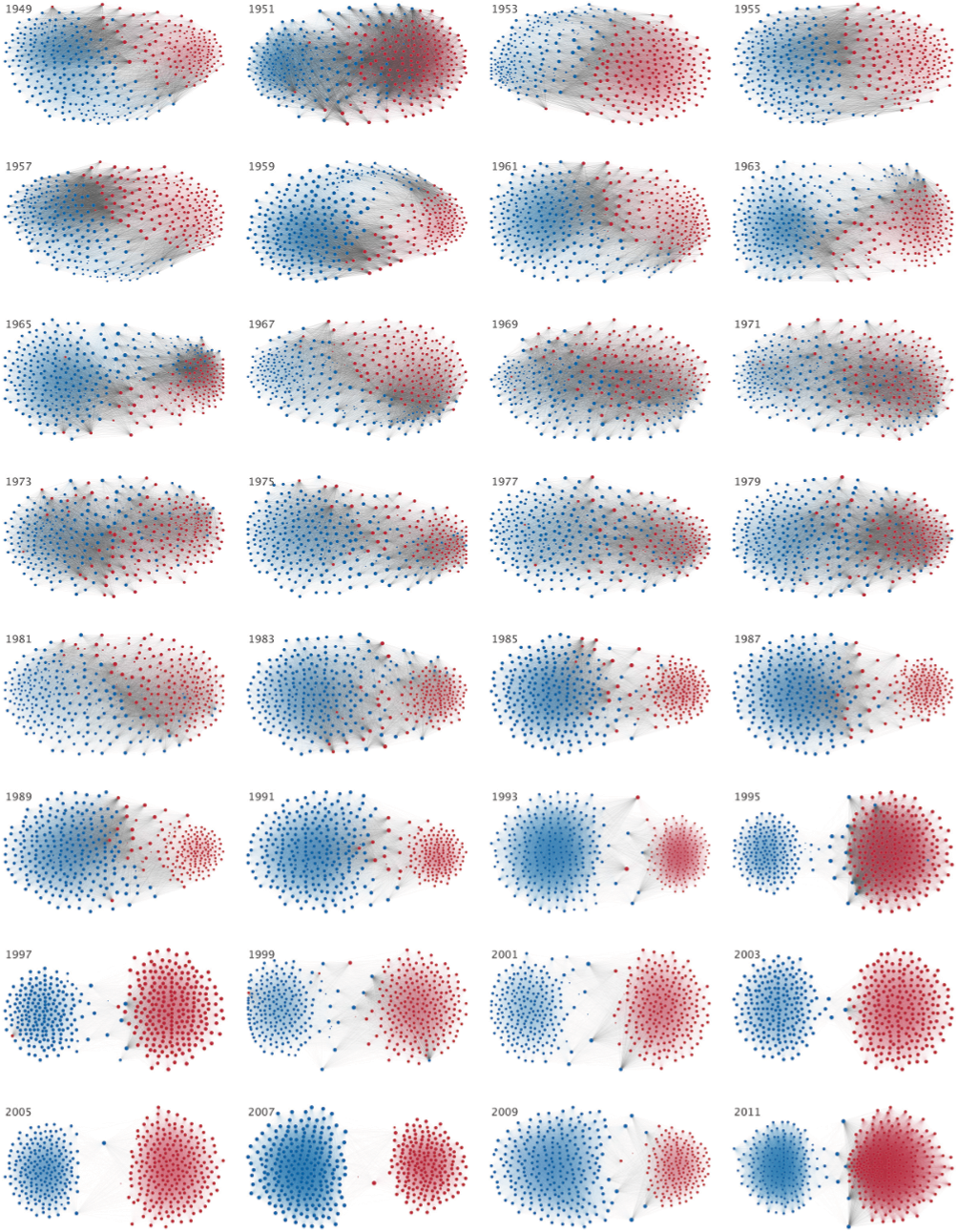
Figure 6: Division of Democrat and Republican party members over time [55]. “Each member of the U.S. House of Representatives from 1949-2012 is drawn as a single node. Republican (R) representatives are in red and Democrat (D) representatives are in blue; party affiliation changes are not reflected. Edges are drawn between members who agree above the Congress’ threshold value of votes. The threshold value is the number of agreements where any pair exhibiting this number of agreements is equally likely to be comprised of two members of the same party (e.g. D-D or R-R), or a cross-party pair (e.g. D-R). Each node is sized relative to its total number of connections; edges are thicker if the pair agrees on more votes. The starting year of each 2-year Congress is written above the network”

4.7 Mini discussion

Although the original bounded confidence model was built using the assumption of homophily to explain social interactions, its sharp cut off point, which determines who may interact with whom, does not exist in real life. However, recent technological and cultural changes and the rapidly increasing speed of life have resulted in an environment in which vast quantities of information are sent and received via online media whose algorithms are optimized to learn from the actions of users and to show them topics or ideas in which they are already interested and with which they already agree. Hence, the news items, tweets, posts and likes that are seen by individuals will be overwhelmingly likely to support and agree with their current opinions, and homophily is the side effect of such algorithms. This idea is presented in Ref. [56] along with simulation results. In paper [56], the DW version of the bounded confidence model (i.e., with pairwise interaction) is modified so that the probability of interaction between two agents, whose opinions lie within the confidence radius, is dependent on the difference of their opinions. The smaller the difference, the greater the probability of interaction between randomly chosen pairs. In this model, after agent $i$ is chosen randomly, the interaction partner is then chosen from among agents $j$ for whom $|d_{ji}|=|o_{j}-o_{i}|<r$ with probability $p_{i}(j)=\frac{|d_{ij}|^{-\gamma}}{\sum_{k\neq i}|d_{ik}|^{-\gamma}}$. The parameter $\gamma$ tunes the degree of homophily or bias. The effects of such modification are the following:

• The system will end up with fragmented groups of agents, whereas in the original model, the same settings resulted in consensus.

• The time needed to reach steady state or equilibrium is significantly increased.

• The average distance between opinions is also increased.

An interesting idea is presented in Pilyugin and Campi [57] where the “reinforcement theory” of the social sciences meets opinion dynamics. He used the update rule $o_{i}^{(t+1)}=o_{i}^{(t+1)}+\frac{\mu}{|N_{i}|}\sum_{j\in N_{i}}o_{j}^{(t)}$ in the bounded confidence fashion in opinion space $\mathcal{O}=[-1,1]$. He remarked the fact that since $\frac{\mu}{|N_{i}|}\sum_{j\in N_{i}}o_{j}^{(t)}$ includes the agent $i$ itself, “$i$ in absence of counter-arguments, tends to strengthen her/his own initial opinion” and “drift towards a higher level of belief in the absence of opposite voices,” which is in agreement with reinforcement theory. Of course the update rule can violate the boundaries. (Imagine agent $i$ with no one in its confidence interval. It will strengthen its own opinion.) So, the new opinions will have to be clamped. To be precise, the update rule actually is $o_{i}^{(t+1)}=clamp(o_{i}^{(t+1)}+\frac{\mu}{|N_{i}|}\sum_{j\in N_{i}}o_{j}^{(t)})$.

The operator that maps $\mathbf{o^{(t)}}=[o_{1}^{(t)},o_{2}^{(t)},\cdots,o_{N}^{(t)}]$ to $\mathbf{o^{(t+1)}}$ was considered in Ref. [57] and it is shown that the operator’s basic fixed points are asymptotically stable and the nonbasic fixed points are unstable. Basic fixed points are of the form $[-1,-1,\cdots,-1,1,\cdots,1]$. For a discussion of nonbasic fixed points, please see Ref. [57]. It was also shown that if the confidence radius is $r\leq 0.5$ then the trajectories of the operator above will go to fixed points. Pilyugin viewed this continuous dynamic model as a tool for analyzing the voting process in a system in which only one outcome, either 1 or -1, is allowed; by the use of simulations, he arrived at the conclusion that the outcome of elections can vary depending on the level of interaction of society, i.e. depending on the size of the confidence radius.

Another work that includes a novel modification of the DW model is Ref. [58], in which the learning rate is a function of opinion differences in single interactions. Using this scenario. Reference [58] studied convergence time and the probability of consensus via Monte Carlo simulations.

We would like to flashback to the question posed in the Sec. 1 about the limitations that prevent people from interacting synchronously and introduce two works that address this limitation. Perra and Rocha [59] states, “We are bounded by cognitive and temporal constraints. Our attention is limited.” Because of these limitations, which are ignored in synchronous models, our attention is valuable. Commercial companies or political parties must compete to gain and hold our attention. Social medias, such as Facebook, are utilized to obtain the attention of users for various reasons, such as to increase revenue or to influence voting decisions. Therefore, the information revealed to each user is filtered by machine learning algorithms to increase the likelihood of the desired outcome. Perra and Rocha [59] makes use of three types of filtering; random filtering, time ordering and the accumulation of past ideas, likes, etc., expressed by the user‚ to study the filtering effect on opinion dynamics. Perra demonstrated that the distribution of opinions is affected by the filtering algorithm, especially when the filtering is based on the past behaviors of users. The simulations were then applied to three different networks; a random network, a Watts-Strogatz network and a 2D lattice‚ and it was also shown that if social media sends a particular opinion to a fraction of users regularly, such messages can affect their behavior and users can be manipulated toward a given opinion. This result is similar to what we have already seen in other cases for fully-stubborn agents.

The fact that synchronous interactions are unrealistic was also noted by Patterson and Bamieh [60]. They modified the DeGroot model, $\mathbf{O}^{(t+1)}=\mathbf{AO}^{(t)}$, to consider the interaction frequency between agents in the following way:

$$\mathbf{O}^{(t+1)}=\left(\mathbf{I}-\sum_{(i,j)\in E}\delta_{ij}^{(t)}\mathbf{A}_{ij}\mathbf{L}_{ij}\right)\mathbf{O}^{(t)}$$ (51)

Please note that $\mathbf{A}_{ij}$ are scalars, (i.e., entries located at the $(i,j)$ position of the weight matrix $\mathbf{A}$), and $\mathbf{L}_{ij}$ is a matrix associated with the edge $(i,j)\in E$ of the graph $\mathcal{G}$. More precisely, the matrix $\mathbf{L}_{ij}$ is associated with the subgraph $\mathcal{G}_{ij}$, which only has the edge $(i,j)$ in it and it is referred to as the weighted Laplacian matrix of the $\mathcal{G}_{ij}$, and one can write $\mathbf{A}=\mathbf{I}-\sum_{(i,j)\in E}\mathbf{L}_{ij}$. Furthermore, the $\delta_{ij}^{(t)}$’s are independent random variables taking a value of 1 with probability $p_{ij}$ and a value of 0 with probability $1-p_{ij}$. The interaction frequency is captured by a probability of communication. Furthermore, the consensus conditions and efficiency (i.e., convergence rate) were analyzed along with the network modification to improve the efficiency of both the classical DeGroot model and the altered DeGroot model described above.

4.8 Extensions and related models

Before moving on to the next section we list some interesting bounded confidence models.

A recent bounded confidence model is found in Ref. [61], in which opinions lie in $\mathbf{o_{i}}\in\mathbb{R}^{d}$. The interactions are pairwise; a random agent $i$, selected from a fully connected graph, chooses a random neighbor, and if $||\mathbf{o_{i}}^{(t)}-\mathbf{o_{j}}^{(t)}||_{2}<r$, then both agents will converge to the mean of their opinions in each dimension, i.e., $\mathbf{o_{i}}^{(t+1)}=\mathbf{o_{j}}^{(t+1)}=\frac{1}{2}(\mathbf{o_{i}}^{(t)}+\mathbf{o_{j}}^{(t)})$, i.e., the learning rate is $0.5$. Therefore, if the matrix of opinions of all $N$ agents is given by $\mathbf{O}\in\mathbb{R}^{N\times d}$, where each row represents an agent, then at each time step two rows will become identical. Let the graph be a fully connected one, and define $\mathbf{W}(i,j,t)=\mathbf{I}-\frac{1}{2}(\mathbf{e_{i}}-\mathbf{e_{j}})(\mathbf{e_{i}}-\mathbf{e_{j}})^{T}$, which is a matrix with $0.5$ at positions $(i,i),\>(i,j),\>(j,i),\>(j,j)$ and zeros elsewhere, so that $\mathbf{O}^{(t+1)}=\mathbf{W}(i,j,t)\mathbf{O}^{(t)}$ defines the update after the interaction between $i$ and $j$. Then the equilibrium point of the system, $\mathbf{O^{*}}$, satisfies $\mathbf{O^{*}}=\mathbf{W}(i,j,t)\mathbf{O^{*}}$ for any $t\geq T^{*}$. For the system mentioned above at equilibrium, any two agents $i$ and $j$ will either be at consensus or separated by a distance greater than the confidence radius $r$:

$\mathbf{o_{i}}^{*}=\mathbf{o_{j}}^{*}$       or       $||\mathbf{o_{i}}^{*}-\mathbf{o_{j}}^{*}||_{2}\geq r$

It has also been shown that the bounded confidence mentioned above, with learning rate $0.5$, for any initial opinion in $\mathbb{R}^{d}$, will almost surely reach such an equilibrium state. This intuitive result is also obtained in Ref. [33] and Refs. [62, 63, 37] for different versions of bounded confidence models.

In the above system the confidence radius is fixed. Now consider an iterative version of the system, whereby the game is repeated as follows: 1. initialize $\mathbf{O}^{(0)}$, and run the game until the system reaches its equilibrium; 2. at this point, use the equilibrium state as the initial state of the next round, with the confidence radius increased by $\Delta r$, so that for the second round we have $r\mathrel{\mathop{\mathchar 58\relax}}=r+\Delta r$. The iterations can be repeated until a predefined maximum confidence $r_{max}$ is reached. This approach allows the number of clusters to be reduced as the confidence radius is increased.

Two interesting ideas that are related to HK-type dynamics were introduced in this model in [64]. For the first novel idea, let the opinion space be $\mathbb{R}^{k}$, let agents $i$ and $j$ communicate whenever $||o_{i}-o_{j}||_{2}\leq 1$, and define the update rule by $o_{i}^{(t+1)}=(1-\lambda_{i})o_{i}^{(t)}+\frac{\lambda_{i}}{|N_{i}|}\sum_{j\in N_{i}}o_{j}^{(t)}$, where $\lambda_{i}\in[0,1]$ is called inertial (note that self-loops exist in the above equation). It has been shown that such a system converges asymptotically when $\lambda_{i}\in\{0,1\}$, and in one dimension the convergence is exponentially fast. The second novel idea involves an anchored HK system. In this system each agent is identified by $z_{i}=(o_{i}^{(t)},y_{i})$, where $o_{i}^{(t)}\in\mathbb{R}^{k}$ is the moving part of agent $i$ and $y_{i}\in\mathbb{R}^{\hat{k}}$ is the fixed part. Two agents interact whenever $||z_{i}^{(t)}-z_{j}^{(t)}||_{2}\leq r$, for some value of $r$. The fixed part plays a role only in the communication graph and determines whether $i$ and $j$ are neighbors at any given time. The authors of  [64] show that an anchored system like this has a symmetric heterogeneous HK equivalent. (A symmetric heterogeneous HK system is a system in which each edge is assigned its own confidence radius; in other words, agents $i$ and $j$ each have their own confidence radius when they interact with each other.) We would also like to mention that in almost all models/papers, the equilibrium of the system when the interactions stop is determined as if agents have global knowledge of the system. Xie et al. [65] built on the work of others [66, 67] and considers a local stopping criteria in a system where agents are only aware of their neighbors. In most of the literature, the dynamics and the simulations stop with a knowledge of the global state of the network, or after a large number of steps have been taken. Such results are questionable when modeling actual systems with real-life agents that need not know the global state of the network they live in. In addition, the asymptotic state of the network also depends on topology and the initial state of the system, and computing the needed number of iterations may be hard, impossible or unrealistic for time varying networks.

5 Further Work and Further Questions

In this section we provide more models worthy of notice and end the paper with questions that are not studied yet.

5.1 Other works

In the following subsections we include newly developed models, influential works that are not variation of DeGroot or bounded-confidence models and provide pointers so more works of researchers.

Let us start with models supporting the repulsive behaviors that exist in real life–whether in human interactions, the interactions of gas molecules or birds flying together.

Noorazar et al. [24] introduced a rich and flexible opinion dynamic model inspired by energy functionals from physics. In this model two interacting agents have an energy between them that is a function of their opinion difference. The update rule is given by

$$\left\{\begin{array}[]{lr}o_{i}^{(t+1)}&=o_{i}^{(t)}-\frac{\mu}{2}\>\psi^{\prime}(|d_{ij}^{(t)}|)\>\frac{d_{ij}^{(t)}}{|d_{ij}^{(t)}|}\vspace{.1in}\\ o_{j}^{(t+1)}&=o_{j}^{(t)}+\frac{\mu}{2}\psi^{\prime}(|d_{ij}^{(t)}|)\>\frac{d_{ij}^{(t)}}{|d_{ij}^{(t)}|}\end{array}\right.$$ (52)

where $\psi$ is the energy function and $\mu$ is the learning rate. In this model, potential functions can be agent specific. Assigning potential functions to edges (i.e., defining interaction-partner-dependent potential functions) will make the system highly complicated and flexible.

It has been noticed that, for example, the DW model is a special case of this model if the $\psi$ is given by Fig. 7(a), in which case we have $\psi(x)=x^{2}$ when $x<0.5$, and $\psi^{\prime}(x)=0$ beyond that. By changing the flat part of Fig. 7(a) to a decreasing function, as shown in Fig. 7(b), we can easily obtain repulsive behavior. We also note that: One can also take the BCM potential function, shown in Fig. 7(a), and smooth out the function at $\tau$ so that it is differentiable, thus solving the problem of the sharp transition between acceptance and rejection in the BC model.

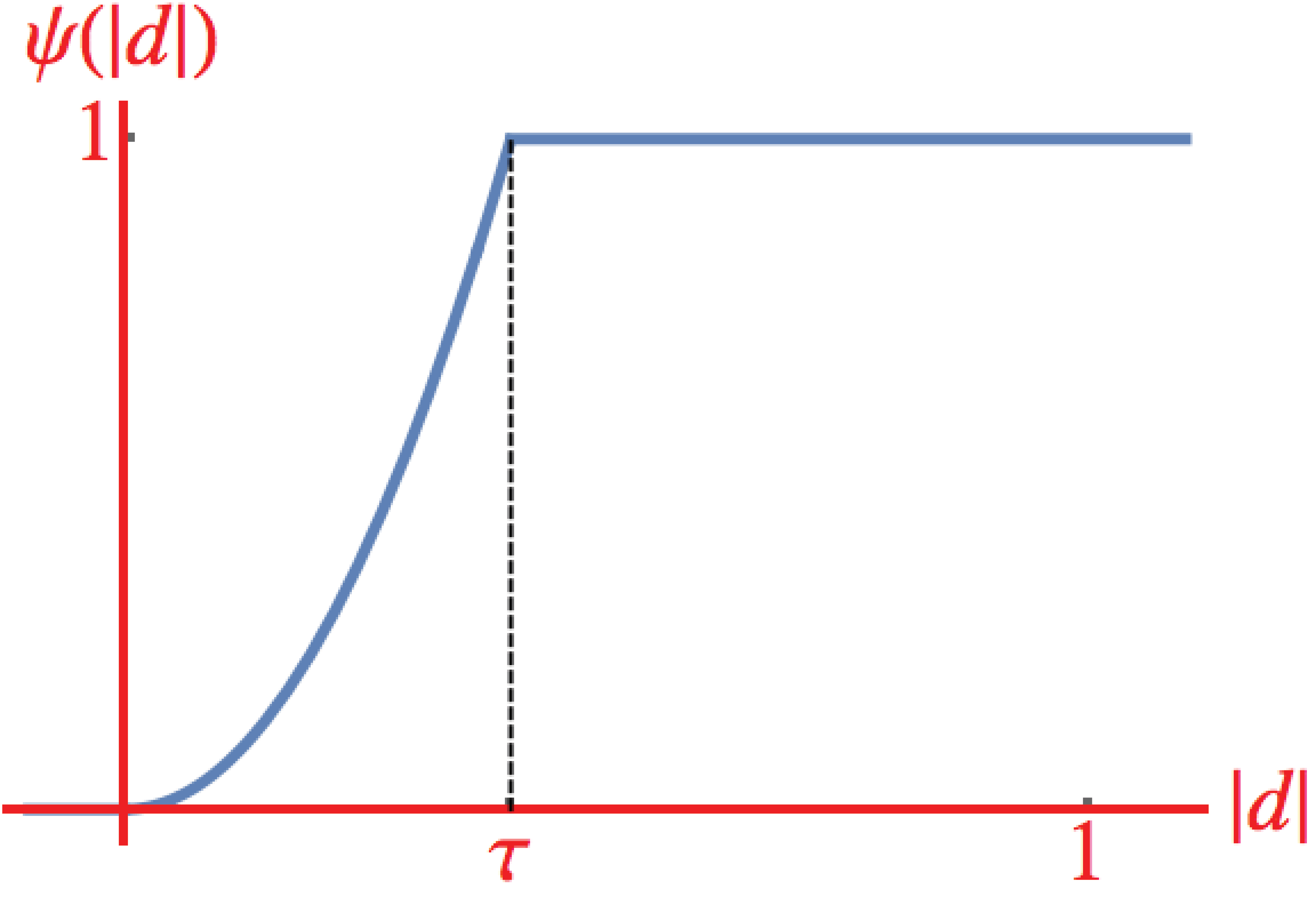
(a) BCM potential function

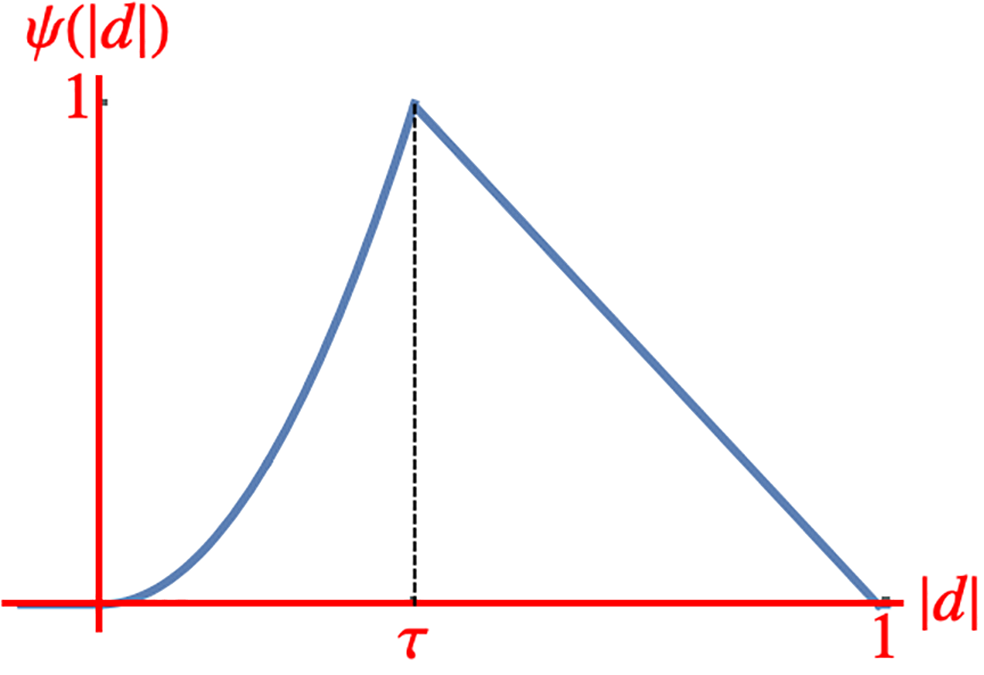
(b) BCM repulsive

Figure 7: BCM potential function and an alternative. Using 7(a) as the potential function in Ref. [24] induces the bounded confidence model and using 7(b) will cause the regions of indifference in BC models be replaced with repulsive behavior.

Two other simple potential functions are given below in Fig. 8. The tent potential function, Fig. 8(a), supports both attraction and repulsion. Whether attraction or repulsion occurs depends on the ‚ opinion difference‚ which can be thought of as a time-varying topology that is not arbitrarily random, as it was in Ref. [68]. The attraction or repulsion, i.e., friendship and antagonism, at any given time is governed by the potential function, but the randomness of the relationship between a pair of agents is due to random pairwise interactions that have led the two agents to their current positions. Finally, Fig. 8(b), is the flat top tent potential function, which gives an agent the option of behaving in one of three modes; attraction, indifference and repulsion, making the model even richer and more flexible.

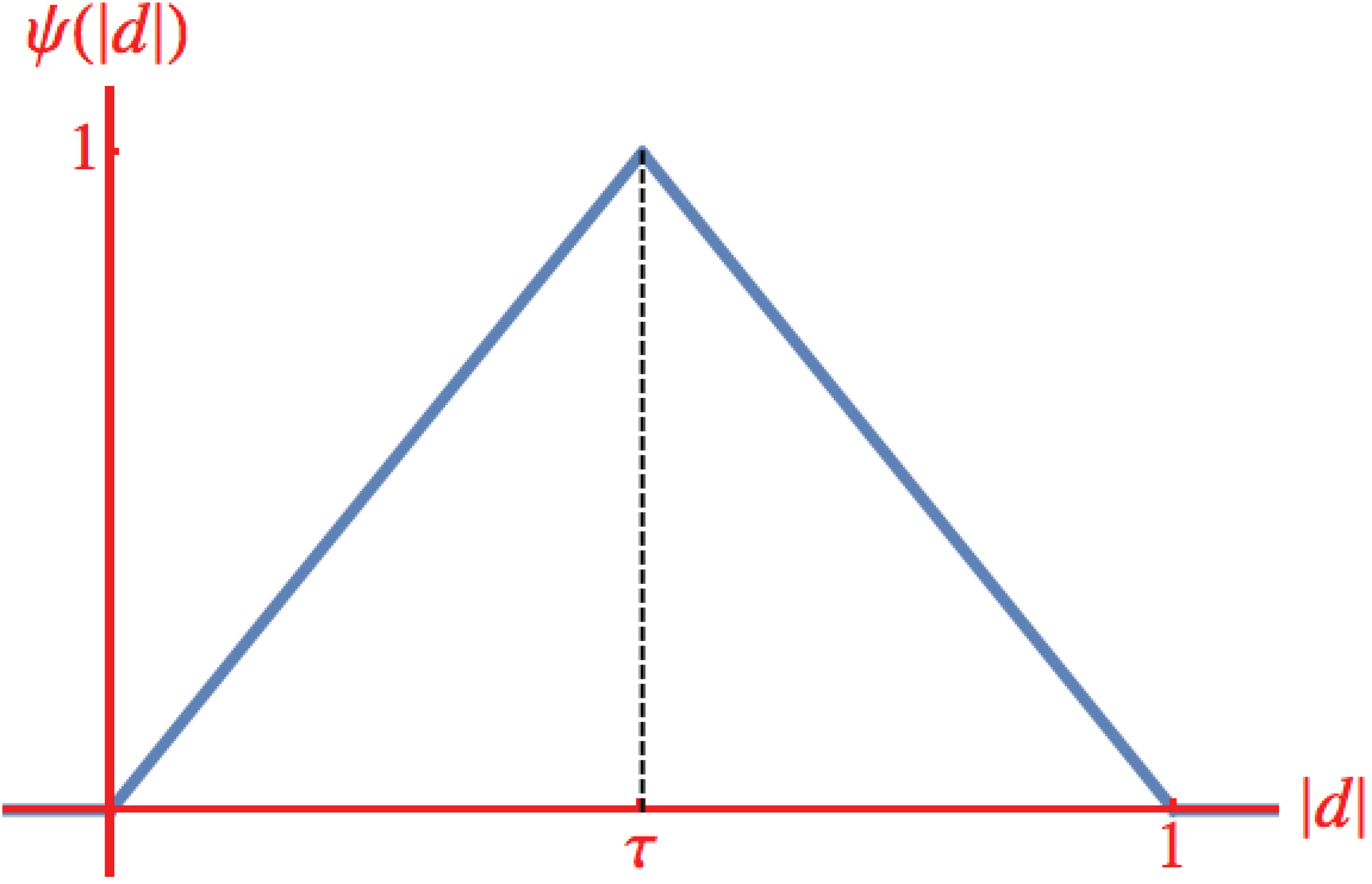
(a) tent function

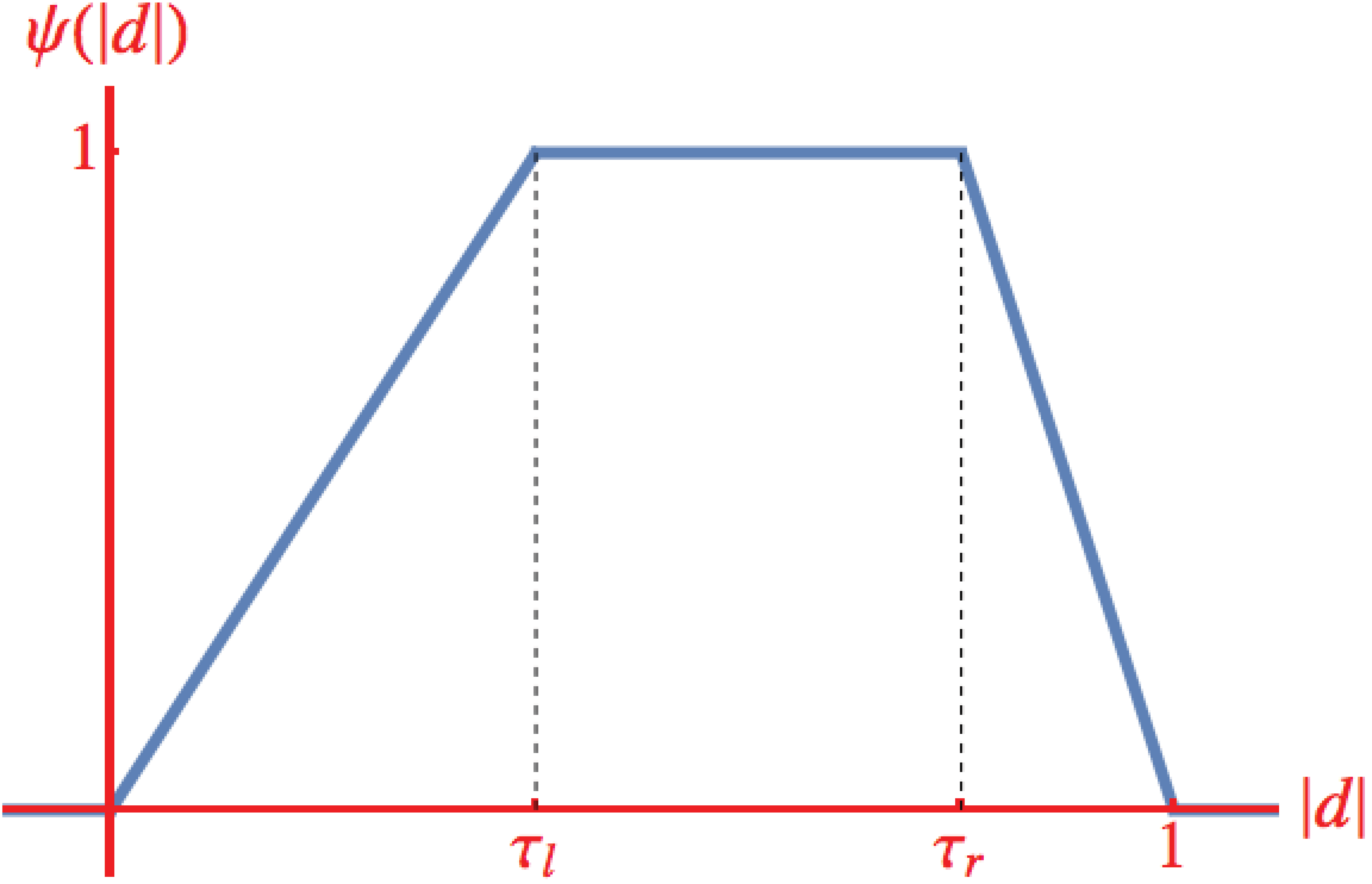
(b) skewed flat top tent

Figure 8: Potential function examples

Besides discussing repulsive behavior, Ref. [24] also covers the modeling of interrelated topics in both discrete and continuous topic space.

The second class of models that support repulsive behavior is based on the idea of balanced networks. Let us start with the definition of structurally balanced networks.

Definition 5.1.

Consider a fully-connected network of 3 agents where each edge between them is assigned a relationship status of either friend (+) or adversary (-) (See Fig. LABEL:fig:figbalance.) The 3-agent fully-connected network is said to be structurally balanced if it has either 1 or 3 positive signs (the product of the 3 signs is positive in these cases). A network with more than $N=3$ agents is said to be structurally balanced if every fully connected 3-node subgraph in it is structurally balanced.

An immediate consequence of the above definition is that a structurally balanced network can be divided into two subgroups where the relationships within subgroups are friendly and the relationships between subgroups (any two agents from different subgroups) are adversarial. Moreover, it is assumed that any pair of connected agents are aware of their relationship, and, their relationship is either friendly or adversarial.

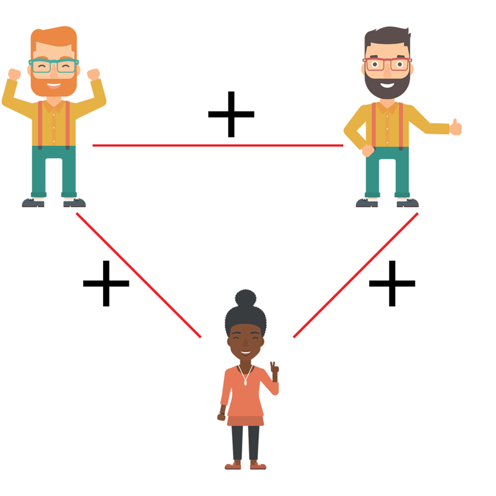
(a) Everyone is friendly: balanced

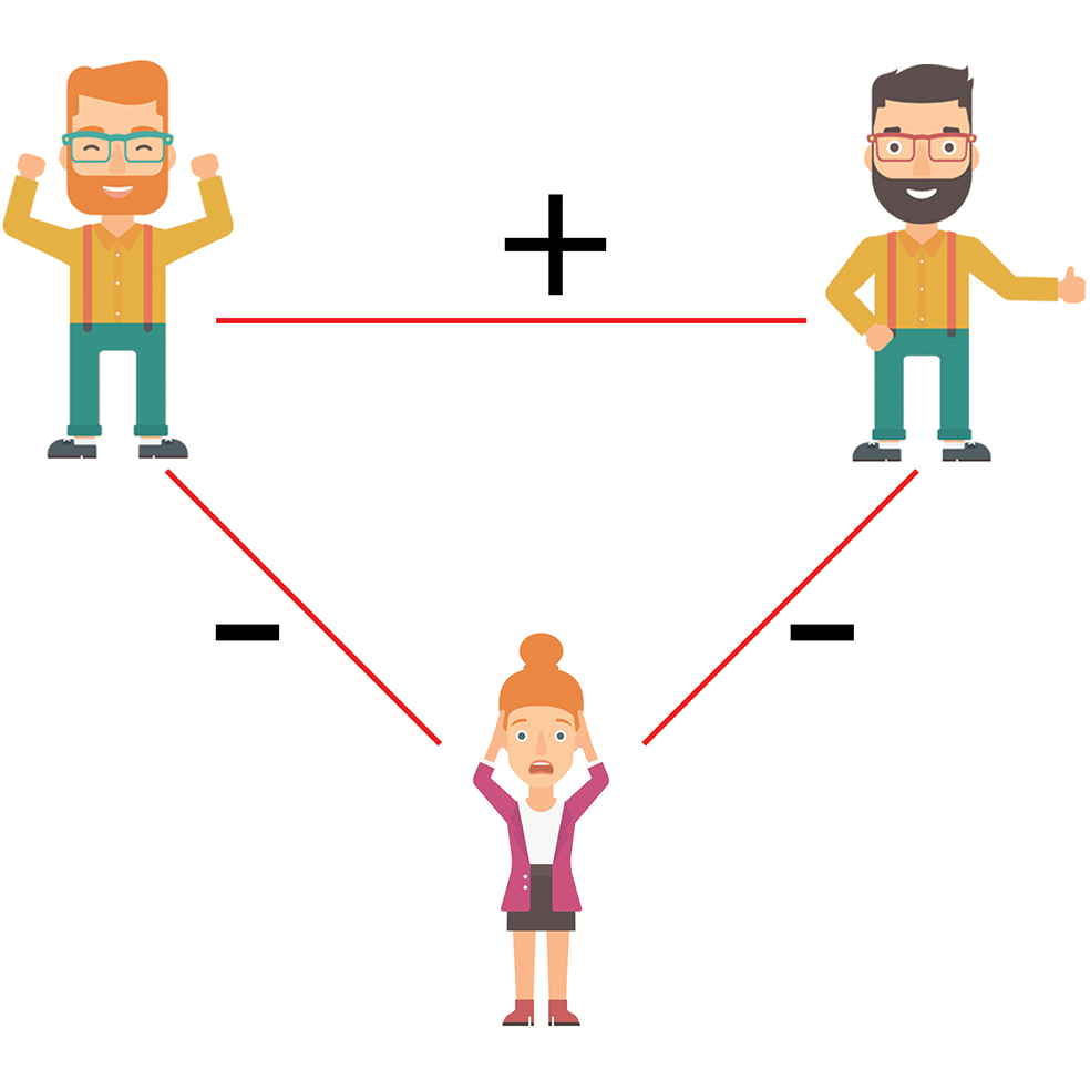
(b) Two friends have a mutual adversary: balanced

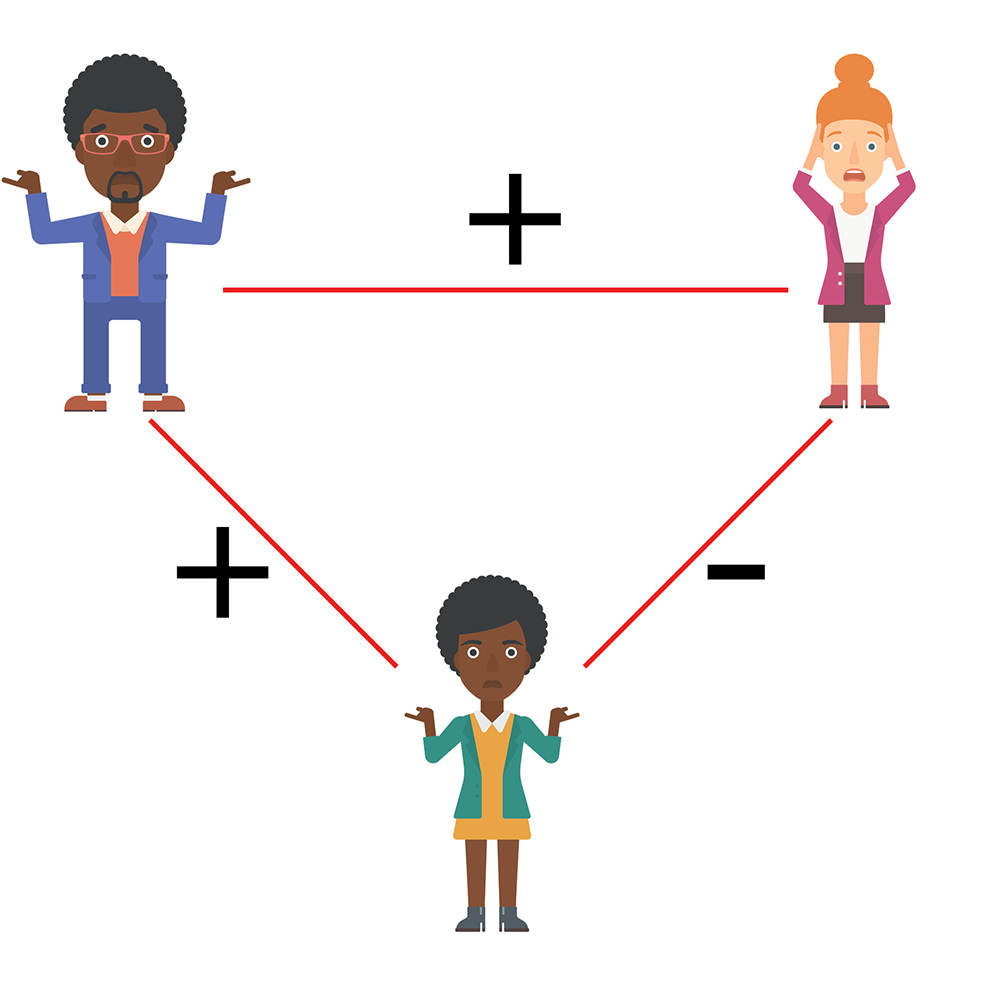
(c) The antagonistic relationship may effect the friendship relationships: imbalanced

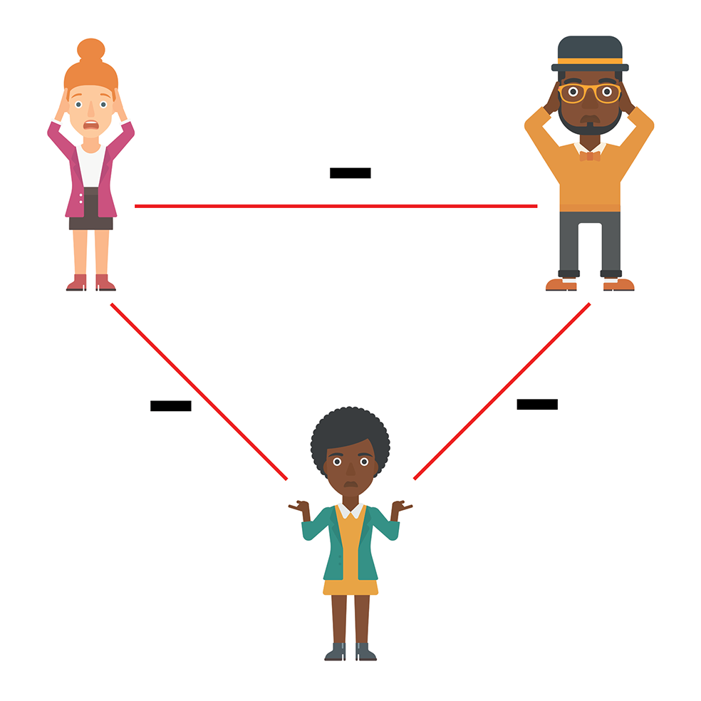
(d) All enemies: imbalanced

Figure 9: Structural balance among three agents. Balance requires either 1 or 3 friendship relationships, otherwise the structure is imbalanced. A graph with more than $N=3$ agents is balanced if all of its fully connected 3-agent subgraphs are balanced.

Altafini [4] used theories presented in Refs. [[69, 70]] to model a structurally balanced community with a dynamical system approach; namely, a monotone dynamical system, with its well-known properties, was used to model this type of social community. A structurally balanced network is a community that is divided into two antagonistic sub-communities, and agents within a given sub-community are friendly/cooperative and have a positive influence on each other, whereas agents from different sub-communities are adversaries/antagonistic. In this model the relationships among agents remain constant‚ they are either on good terms or they are adversaries. Relationships are also independent of opinions or opinion differences; it is therefore possible for two agents with widely different opinions to attract each other, and agents with close opinions need not attract each other. The nature of these relationships is expressed via constant signs on the edges: a positive sign indicates friendship and a negative sign, antagonism. Friends, who by definition belong to the same sub-community, are connected to each other by edges with positive weights assigned to them, and inter-community edges are assigned negative weights to model antagonism.

Clearly, the structure of the graph makes the final state of the system predictable: polarization is inevitable unless all members of a given sub-population decide to join the other party.

The edge weights that define the relationships between pairs of agents are translated into directional derivatives of the functional defining the dynamics of the system. See Ref. [4] for more details. Later the model is extended to explain how it is possible for agents in such a system to reach opinions of equal size but opposite sign [71]. In the works mentioned so far in this section, opinions belong to $\mathcal{O}=\mathbb{R}$. Later, Altifani [71] studied the consensus problem using this model and Proskurnikov et al. [68] investigated the use of an arbitrary time-varying signed graph with this model.

Proskurnikov et al. [68] built on Altafini’s model using a network that is not static; specifically it is not required to be structurally balanced at the beginning. Such a system can reach a structurally balanced state at some time $t>0$. For further reading on the origins of evolving networks and the conditions for reaching a structurally balanced topology, please see Ref. [68].

Altafini and Ceragioli [72] extended his work to include the case of repulsive behavior as well. In what follows, we briefly explain his recent work. Consider an opinion dynamic with opinion space $\mathcal{O}=\mathbb{R}$ or $\mathcal{O}=[-1,1]$, or any opinion space, really, which contains a point of neutrality (in the cases mentioned above, zero would be the neutrality point). Positive opinions would be the strength of agreement on a given topic and negative ones would be the strength of opposition to it. Altafini and Ceragioli [72] argued that agents with opinions near zero might fall within each other’s confidence radiuses. However, moving from one side of zero to the other is not easy in the real world, and does not happen frequently. Hence, they added three separate components to his earlier work; incorporated into the bounded confidence model, these additions resulted in three new models. In the first model (which is similar to his earlier work) if agents $i$ and $j$ have close opinions that differ in sign, they will be attracted to the opposite of the opinion of the other. In the second model, agents with opinions of opposite signs ignore each other, and in the third, agents whose opinions are close enough and of opposite sign, repel each other. Therefore, opinions in these three models always retain their initial sign during time evolution, and the models are referred to as signed bounded confidence models. These results were motivated by and compared with the results of the ordinary bounded confidence model with continuous time (the derivation of this model is shown in interesting works referenced in Ref. [72]. Zhang and Chen [73] built on earlier work of their own [74] along with Altafini’s [71] work and designed an “output feedback control law” to study consensus in networks that included antagonistic interactions in conjunction with strongly connected graphs, spanning tree graphs and graphs with spanning trees. His work provided results for such scenarios when the network is structurally balanced or unbalanced.

Some recent interesting work related to antagonism includes the following: Yang and Song [75] mapped social networks onto electrical networks, with each interaction node between agents being mapped to a link in an electrical network and with the resistance (or rather conductivity) of each link representing the interaction/influence weight of the agents on each other. She used the effective conductance (EC) concept to measure the direct and indirect relationships of a given pair of agents whose interactions are defined by a DeGroot-type update rule: $o_{i}^{(t+1)}=o_{i}^{(t)}+\lambda\sum_{j\in N_{\bar{i}}}w_{ij}(o_{j}^{(t)}-o_{i}^{(t)})$. In the update rule it is assumed that $w_{ij}=w_{ji}\in\mathbb{R}$. Hence, this model also assumed antagonistic interactions with no assumption on the structure of the graph, and a positive EC that would indicate, overall, the direct and indirect nature of the interactions between a pair of agents. The consensus criteria for this model were considered as well; for more details please see [75] and references therein. Meng et al. [76] considered an antagonistic dynamic on a network with agents that are separated into two groups, and with a topology that switched between $M$ finite digraphs. Meng studied the behavior of such systems by lifting restrictions such as the structural balance we saw in previous models. For further discussion please see Ref. [76].

Antal et al. [77, 78] considers a network with two types of relationship, friendly and antagonistic, in which relationships change in order to turn imbalanced triads into balanced ones. Refs. [77, 78] are not about opinion dynamics, but perhaps this line of work can be utilized with opinion dynamics to explore novel questions.

To the best of our knowledge, Ref. [44] is the first to introduce the individuality tendency to the literature. When the individuality tendency is added to the model of Durkheim, the update rule becomes:

$$o_{i}^{(t+1)}=o_{i}^{(t)}+\xi_{i}^{(t)}+\frac{\sum_{j\neq i}(o_{j}^{(t)}-o_{i}^{(t)})w_{ij}^{(t)}}{\sum_{j\neq i}w_{ij}^{(t)}}$$ (53)

where the influence weights are adaptive and are functions of the opinion difference between two given agents:

$$w_{ij}^{(t)}=e^{-\frac{|d_{ij}^{(t)}|}{\gamma}}$$ (54)

where $d_{ij}^{(t)}=o_{i}^{(t)}-o_{j}^{(t)}$. The parameter $\gamma$ specifies the level of confidence each agent has in its own opinion. Small $\gamma$ values imply high confidence in the current opinion and that agents are influenced mostly by those with whom they hold similar opinions. The adaptive noise is drawn from a normal distribution with zero mean and its variance is given by ($\xi_{i}^{(t)}\sim N(0,\sigma_{i}^{(t)})$), where

$$\sigma_{i}^{(t)}=s\sum_{j}e^{-|d_{ij}^{(t)}|}$$ (55)

The parameter $s$ is used to manipulate the uniqueness tendency in the model, and the variance $\sigma_{i}^{(t)}$ is larger for agents who find themselves similar to a greater number of other agents.

The Mäs [44] model is motivated by the Durkheim theory of social interactions [79], in which individuals conform to society’s norms while also tending to be unique and different, which fosters the co-existence of many different opinions. The homophily assumption of confidence models is missing here, as an agent is influenced by all other agents. There is also no repulsion or negative influence. And please note that in Eq. 53, agent $i$ is the only one updating its opinion, that is, in the simulations a random agent is chosen to update its opinion. Such updates are neither pairwise nor synchronous. In the Mäs [44] paper, simulations start from a state of total consensus in which all agents hold the exact same opinion and in the 2-dimensional space of integrating and disintegrating parameters, $(\gamma,s)$, there is an extensive area for which different meta-stable clusters co-exist, while in the other areas various types of quasi-consensus or total chaos is observed.

The Mäs’s results were obtained from a simulation on a fully connected network to explain clustering, i.e., to explain the lack of complete consensus at the end of long simulation runs. The motivation was the need to explain the co-existence of different opinions in a network where all agents may interact with each other, as opposed to networks that contain artificial constraints on the topology of the network through disconnections or loosely connected subgraphs [13]. Mäs’s modification more closely approximates connectivity in the real world, which now includes the internet and social media.

We mentioned before, humans do not possess a sharp decision boundary beyond which they ignore others, as seen in the DW model. Baccelli et al. [80] tried to address this issue by incorporating the effect of probabilistic opinion exchange between agents; in other words, they attempted to smooth out the sharp transition between interacting with and ignoring others in the DW model. The model includes a random internal thought for each agent. The random internal thought has an expanding effect. Their modifications included allowing agents to ignore those whose opinions are close to their own as well as to learn from those who did not think like them. The update rule for these modifications is given as follows:

$$\begin{split}\begin{cases}o_{i}^{(t+1)}=\begin{cases}o_{i}^{(t)}+\xi_{i}^{(t)}+w_{ij}(o_{j}^{(t)}-o_{i}^{(t)})&\text{if $U_{i,j}^{(t)}=1$,}\\ o_{i}^{(t)}+\xi_{i}^{(t)}&\text{o.w.}\\ \end{cases},&\\ \\ o_{j}^{(t+1)}=\begin{cases}o_{j}^{(t)}+\xi_{j}^{(t)}+w_{ji}(o_{i}^{(t)}-o_{j}^{(t)})&\text{if $U_{j,i}^{(t)}=1$,}\\ o_{j}^{(t)}+\xi_{j}^{(t)}&\text{o.w.}\\ \end{cases}&\\ \\ \hskip 2.84544pto_{k}^{(t+1)}=o_{k}^{(t)}+\xi_{k}^{(t)},k\not\in\{i,j\}\end{cases}\end{split}$$ (56)

where we must note that:

• $U_{i,j}^{(t)}\in\{0,1\}$ is a random variable indicating whether agent $i$ is influenced by agent $j$ or not; it is a function of their opinion difference. So, when agent $i$ is not influenced by agent $j$, agent $j$ is simply ignored. This is where stochasticity comes in:

  $$p(U_{i,j}^{(t)}=1)=f_{i,j}(|o_{j}^{(t)}-o_{i}^{(t)}|)\mathrel{\mathop{\mathchar 58\relax}}\mathbb{R}^{+}\rightarrow[0,0.5)$$ (57)

• $\xi_{k}^{(t)}$ is the noise (“endogenous belief or bias”).

• $w_{ij}\in(0,0.5]$ is the influence weight of agent $j$ on agent $i$.

• All agents subject to Eq. 56, regardless of whether they are participating in an interaction or not, will have internal thoughts, i.e., noise that is added to all agents at any given time $t$.

• The opinion space in the Eq. (56) is $\mathcal{O}=\mathbb{R}$. However, in Ref. [80] the model is restricted to $\mathcal{O}=\mathbb{Z}$, and consequently the update rules given by Eq. (56) are modified by a rounding method like ceiling or flooring or else.

Baccelli et al. [80] included a stability or weak consensus definition in their paper that will not be covered here, due to lack of space. (The idea is that “if all agents move to infinity while remaining close to each other, the society is stable”.) However, their work showed that it is sufficient to have an agent in the network with high influence on all other agents to reach a weak consensus. Similarly, it is possible to reach a weak consensus if there is a pathway of strong influences from one agent to another.

Managing consensus or preventing a community from reaching a consensus has attracted the attention of researchers. A recent paper [81] with a basis in control theory employs a novel idea to managing and controlling consensus. The opinions in this paper are in $\mathbb{R}^{n}$, and the update rule is given by $o_{i}^{(t+1)}=u_{i}^{(t)}+\sum_{j=1}^{N}w_{ij}o_{j}^{(t)}$, where $u_{i}^{(t)}$ is the pay-off of a repeated game between agent $i$ and an external source. The second term, like any other averaging scheme, made sure the convex hull of states shrank as time passed, or as the authors put it, the “space averaging process reduces the total squared distance.” The conditions under which such a system converges to a predefined set (which very well may consist of only one element) based on the iteration of games with vector pay-offs was addressed in Ref. [81] with a level of detail that is beyond the scope of this paper.

Another relatively recent work [10] focused on opinion dynamics systems controlled by a fully-stubborn agent. This paper assumed the influence weights depended on both the current state of the agents and time. In this work fully-stubborn agents influence other agents with an influence function but are not influenced in return. Unlike previous bounded confidence models, which assume the influence stops when the opinion distance is greater than some threshold, the model in this paper included “other shapes for the dependency between influence strength and opinion distance.” It also generalized the time-invariant dynamics associated with fully-stubborn agents to a time-dependent dynamic model. The model converged because it required agents to gather around the fully-stubborn agent in finite time, and the fully-stubborn then influenced the other agents to adopt the target consensus value. Another work with a novel idea uses one strategic-agent to maximize the number of agents that fall within a given interval is Ref. [82]. Tools such as those presented in these papers can be utilized to target retail consumers or voters in political elections by both spreading misinformation and combating it.

In addition to the analytically tractable DeGroot and bounded confidence models we looked at in detail in this paper, there are simulation driven approachs to understanding models [83, 84, 85, 86, 87, 88]. This allows for more realistic communication patterns (e.g., pairwise interactions) as well as heterogeneous agent behaviors. Agent-based and Monte Carlo simulations are commonly employed in this case. Agents could have different influence on each other [89], or different topics may be interrelated [24, 90]. In order to introduce a specific kind of agents’ internal thoughts, the tendency for individuality was introduced by [44] in which agents try to be different when uniformity in a group increases, and later this idea was applied with agents’ having a memory [91], where their uniqueness tends to be more in the opposite direction of their community’s movement direction.

There are also analytical approaches for studying opinion formation that are based on well-known Boltzmann-type equations of dilute gases [92, 93, 94, 95, 96, 97]. The advantage of this approach is that well established methods from statistical physics can be used to study the evolution of densities/distribution of agents/opinion in regions of opinion space in the time limit. However, some aspects of physical systems are removed when applied to agents’ interactions. Some of the simplifications, for example, are: interaction among agents could happen with very few agents whereas for molecules of gases to interact they have to have high density, or, in opinion dynamics, limitations are imposed around opinion space boundaries [98] whereas gas molecules interact also with the walls of the environment they live in. The application of integro-differential equations of Boltzmann type are not limited to opinion dynamics, they are also applied to other areas such as economics and wealth distribution for which a gentle introduction source is [99]. A relatively recent work in this area [100] shows how nonlinear dynamics of diffusion and anti-diffusion can create clusters, where formation of clusters and their attributes are one of the challenges of the field as of today.

Consensus formation has of course attracted quite a bit of attention due to its practical impact. Given the invention of the Internet, social media and such, the connectivity among people has increased and we observe polarizations frequently. Hence, consensus might not be the most interesting limit state that systems may reach after all.

If a decision is to be made by a group of people, the majority vote models are more suitable where consensus may not occur, but a decision is made. Research about group decision making has also recently received attention [101, 102], with focus on consensus [103], decision making on the web [104], and with presence of non-cooperative agents [105], which the aformentioned subject is not studied much. Please take a look at Ref. [106] for a recent survey of research about decision making.

In some models [38, 4, 71, 68, 107, 91] agents do not simply ignore other agents with opinions that are too far from their own. In some works [108, 109, 107, 110] evolving networks are considered and in others [15] evolving influences. Another interesting update rule, in Ref. [107], is based on the difference of opinion of a given agent and all of its connection, however, the update takes place, unlike bounded confidence model, when the difference is larger than a threshold $\delta>0$, due to social pressure. It is unlike most developed models, and it may intuitively seem agents will move towards consensus, however, in fact the model allows existence of a spectrum of opinions, $(o-\frac{\delta}{2},o+\frac{\delta}{2})$.

A major contributor to the field is Galam whose work goes back to 1982 [111] and includes binary opinion dynamics, group decision making and more. For example, the idea of inflexible stubborn agents in binary opinion dynamics was introduced in Ref. [112]. We refer the reader to a survey of his works [113] and his book [114] to learn more about opinion dynamics from a sociophysics perspective.

Galam [115] and Biswas et al. [116] both attempted, with different approaches, to explain Trump’s victory in the US presidential election.

While in this work we are focused on real-valued, continuous opinion space, there are binary version of the model [117, 118] for which opinions are restricted to boolean values. Some of these boolean models are inspired by spin systems (e.g., the Ising model) commonly studied in statistical physics [119, 120, 121]. The Ising model is a simplified model of ferromagnetism in which spins are restricted to two orientations and are influenced by their neighbors on a grid. In between continuous and boolean valued opinions are models in which are discrete but more than two choices are available, for example a recent model is suggested by Bolzern et al. [122] which is a Markov chain model. Another model proposed by Martins [123] is defined for a continuous opinion space but agents take discrete actions.

5.2 New Questions

We have only covered part of the work in the area of opinion dynamics, but even if all of the work is considered, much opportunity remains for exploration and creativity. Here are a few questions and directions that seem interesting that, to our knowledge, are mostly open at this time.

1. There is no work that we are aware of in which higher order interactions are considered, where, for example, collections or cliques of $k$ people ($k>2$) are modeled as interacting in a way that is more than just $\frac{k(k-1)}{2}$ simultaneous pairwise interactions, even though some interactions are not reducible to a bunch of pairwise interactions.

2. Little work has been done on the coupling of topics to each other, even though there is the work on topic sequences. A reasonable approach might consider the topics themselves to form a graph or network, with nodes that are topics and edges and cliques that represent interactions. One would then have an opinion space for each agent that is a network of topics. The interaction dynamics between the topic networks for individual agents are mediated by agent-to-agent interactions. While this is much more complicated, it is also much more realistic and still much simpler than the true reality we are trying to model and understand.

3. There is little work we are aware of that explicitly tries to model the effects of time-to-think and the evolution of opinions outside of an interaction. This is related to the effect that deep reading has on people who take the time to think (see Ref. [80] for work that considers opinion-influencing noise occurring outside of interactions, which can be thought of as the effects of internal thoughts. We briefly mentioned it in Sec. 5.1 where the update rule is given by Eq. 56)

4. The evolution of the connections in the network of agents has been considered, but as far as we know, it has not included geophysical movements, normal life cycle changes, and the economics of connections. There is also the issue of trust evolution due to socially/emotionally impactful interactions. While some of these events would be tightly coupled in time with changes in opinions, others would be hard to tie to immediate opinion changes.

5. Consensus in continuous opinion dynamics is usually studied as time goes to infinity, and humans (or their social groups) do not live forever. Is there a better way to define equilibrium given the finite number of interactions that are physically possible in a fixed time period or lifespan?

References

- [1] Jr. French, J. R. P. A formal theory of social power. Psychological Review, 63(3):181–194, 1956.
- [2] Morris DeGroot. Reaching a consensus. Journal of the American Statistical Association, 69(345):118–121, 1974.
- [3] Noah E. Friedkin. A formal theory of social power. The Journal of Mathematical Sociology, 12(2):103–126, 1986.
- [4] C. Altafini. Dynamics of opinion forming in structurally balanced social networks. In Proceedings of the IEEE Conference on Decision and Control, 2012.
- [5] Guillaume Deffuant, David Neau, Frederic Amblard, and Gérard Weisbuch. Mixing beliefs among interacting agents. Advances in Complex Systems, 03(01n04):87–98, 2000.
- [6] Anton V. Proskurnikov and Roberto Tempo. A tutorial on modeling and analysis of dynamic social networks. part ii. Annual Reviews in Control, 45:166–190, 2018.
- [7] Guiyuan Fu, Weidong Zhang, and Zhijun Li. Opinion dynamics of modified hegselmann–krause model in a group-based population with heterogeneous bounded confidence. Physica A: Statistical Mechanics and its Applications, 419:558 – 565, 2015.
- [8] Ye Tian, Peng Jia, Anahita Mirtabatabaei, Long Wang, Noah E. Friedkin, and Francesco Bullo. Social power evolution in influence networks with stubborn individuals. arXiv:1901.08727, 2019.
- [9] Yucheng Dong, Zhaogang Ding, Luis Martínez, and Francisco Herrera. Managing consensus based on leadership in opinion dynamics. Information Sciences, 397-398:187 – 205, 2017.
- [10] Florian Dietrich, Samuel Martin, and Marc Jungers. Control via leadership of opinion dynamics with state and time-dependent interactions. IEEE Transactions on Automatic Control, 63(4):1200–1207, Apr. 2018.
- [11] Noah Friedkin and Eugene Johnsen. Social influence and opinions. Journal of Mathematical Sociology - J MATH SOCIOL, 15:193–206, Jan. 1990.
- [12] Noah Friedkin and Eugene Johnsen. Social Influence Networks and Opinion Change Models of opinion formation. Advances in Group Processes, 16:1–29, Jan. 1999.
- [13] Rainer Hegselmann and Ulrich Krause. Opinion dynamics and bounded confidence: Models, analysis and simulation. Journal of Artificial Societies and Social Simulation, 5(3), 2002.
- [14] Mengbin Ye and Brian David Outram Anderson. Modelling of individual behaviour in the degroot–friedkin self-appraisal dynamics on social networks. In 2019 18th European Control Conference (ECC), pages 2011–2017, Jun. 2019.
- [15] P. Jia, A. MirTabatabaei, N. Friedkin, and F. Bullo. Opinion dynamics and the evolution of social power in influence networks. SIAM Review, 57(3):367–397, 2015.
- [16] Zahra Askarzadeh, Rui Fu, Abhishek Halder, Yongxin Chen, and Tryphon T. Georgiou. Stability Theory of Stochastic Models in Opinion Dynamics. IEEE Transactions on Automatic Control, pages 1–1, apr 2019.
- [17] Roger L. Berger. A necessary and sufficient condition for reaching a consensus using degroot’s method. Journal of the American Statistical Association, 76(374):415–418, 1981.
- [18] Mengbin Ye, Ji Liu, Brian D.O. Anderson, Changbin Yu, and Tamer Başar. Evolution of Social Power in Social Networks with Dynamic Topology. IEEE Transactions on Automatic Control, 63(11):3793–3808, Nov. 2018.
- [19] Noah E. Friedkin, Peng Jia, and Francesco Bullo. A theory of the evolution of social power: Natural trajectories of interpersonal influence systems along issue sequences. Sociological Science, 2016.
- [20] Rediet Abebe, Jon Kleinberg, David Parkes, and Charalampos E. Tsourakakis. Opinion Dynamics with Varying Susceptibility to Persuasion. Jan. 2018.
- [21] T-H. Hubert Chan, Zhibin Liang, and Mauro Sozio. Revisiting opinion dynamics with varying susceptibility to persuasion via non-convex local search. In The World Wide Web Conference, WWW ’19, pages 173–183, New York, NY, USA, 2019. ACM.
- [22] Ye Tian and Long Wang. Opinion dynamics in social networks with stubborn agents: An issue-based perspective. Automatica, 96:213 – 223, 2018.
- [23] S. E. Parsegov, A. V. Proskurnikov, R. Tempo, and N. E. Friedkin. Novel multidimensional models of opinion dynamics in social networks. IEEE Transactions on Automatic Control, 62(5):2270–2285, May 2017.
- [24] Hossein Noorazar, Matthew J. Sottile, and Kevin R. Vixie. An energy-based interaction model for population opinion dynamics with topic couplin. International Journal of Modern Physics C, 29(11):1850115, 2018.
- [25] S E Asch. Effects of group pressure upon the modification and distortion of judgments. In Groups, leadership and men; research in human relations., pages 177–190. Carnegie Press, Oxford, England, 1951.
- [26] Sheng-Wen Wang, Chung-Yuan Huang, and Chuen-Tsai Sun. Modeling self-perception agents in an opinion dynamics propagation society. SIMULATION, 90(3):238–248, 2014.
- [27] Chung-Yuan Huang and Tzai-Hung Wen. A novel private attitude and public opinion dynamics model for simulating pluralistic ignorance and minority influence. Journal of Artificial Societies and Social Simulation, 17(3):8, 2014.
- [28] Francisco J. León-Medina, Jordi Tena-Sánchez, and Francisco J. Miguel. Fakers becoming believers: how opinion dynamics are shaped by preference falsification, impression management and coherence heuristics. Quality & Quantity, Jul. 2019.
- [29] Mengbin Ye, Yuzhen Qin, Alain Govaert, Brian David Outram Anderson, and Ming Cao. An Influence Network Model to Study Discrepancies in Expressed and Private Opinions. Automatica, 107(7):371–381, Sep. 2019.
- [30] Xi Chen, Panayiotis Tsaparas, Jefrey Lijffijt, and Tijl De Bie. Opinion Dynamics with Backfire Effect and Biased Assimilation. Mar. 2019.
- [31] Pranav Dandekar, Ashish Goel, and David T. Lee. Biased assimilation, homophily, and the dynamics of polarization. Proceedings of the National Academy of Sciences, 110(15):5791–5796, 2013.
- [32] Young-Pil Choi, Alessandro Paolucci, and Cristina Pignotti. Consensus of the Hegselmann-Krause opinion formation model with time delay. Sep. 2019.
- [33] Jan Lorenz. A stabilization theorem for dynamics of continuous opinions. Physica A: Statistical Mechanics and its Applications, 355(1):217 – 223, 2005.
- [34] Santo Fortunato. Universality of the threshold for complete consensus for the opinion dynamics of deffaunt et al. International Journal of Modern Physics C, 15(09):1301–1307, 2004.
- [35] Jan Lorenz. Heterogeneous bounds of confidence: Meet, discuss and find consensus! Complexity, 15(4):43–52, Apr. 2010.
- [36] Markus Brede. How does active participation effect consensus: Adaptive network model of opinion dynamics and influence maximizing rewiring. Jun. 2019.
- [37] Ge Chen, Wei Su, Wenjun Mei, and Francesco Bullo. Convergence Properties of the Heterogeneous Deffuant-Weisbuch Model. arXiv:1901.02092, 2019.
- [38] Jiangbo Zhang and Yiguang Hong. Opinion evolution analysis for short-range and long-range deffuant–weisbuch models. Physica A: Statistical Mechanics and its Applications, 392(21):5289 – 5297, 2013.
- [39] Jiangbo Zhang. Opinion limits study for the multi-selection bounded confidence model. Plos One, 14(1):e0210745, 2019.
- [40] Yilun Shang. An agent based model for opinion dynamics with random confidence threshold. Communications in Nonlinear Science and Numerical Simulation, 19(10):3766–3777, 2014.
- [41] Lanchier N. The critical value of the deffuant model equals one half. ALEA Lat Am J Probab Math Stat, 9:383–402, 2012.
- [42] Olle Häggström. A pairwise averaging procedure with application to consensus formation in the deffuant model. Acta Applicandae Mathematicae, 119(1):185–201, Jun. 2012.
- [43] Sébastian Grauwin and Pablo Jensen. Opinion group formation and dynamics: Structures that last from nonlasting entities. Physical Review E - Statistical, Nonlinear, and Soft Matter Physics, 85(6), Jun. 2012.
- [44] Michael Mäs, Andreas Flache, and Dirk Helbing. Individualization as driving force of clustering phenomena in humans. PLoS Computational Biology, 2010.
- [45] Wei Su, Ge Chen, and Yiguang Hong. Noise leads to quasi-consensus of Hegselmann–Krause opinion dynamics. Automatica, 2017.
- [46] Michael Mäs, Andreas Flache, and James A. Kitts. Cultural Integration and Differentiation in Groups and Organizations, pages 71–90. Springer International Publishing, Cham, 2014.
- [47] M. Pineda, R. Toral, and E. Hernández-García. Diffusing opinions in bounded confidence processes. European Physical Journal D, 62(1):109–117, Mar. 2011.
- [48] Miguel Pineda, Raúl Toral, and Emilio Hernández-Garaćia. The noisy hegselmann-krause model for opinion dynamics. European Physical Journal B, 86(12), Dec. 2013.
- [49] Adrián Carro, Raúl Toral, and Maxi San Miguel. The Role of Noise and Initial Conditions in the Asymptotic Solution of a Bounded Confidence, Continuous-Opinion Model. Journal of Statistical Physics, 151(1-2):131–149, 2013.
- [50] Walter Quattrociocchi, Guido Caldarelli, and Antonio Scala. Opinion dynamics on interacting networks: media competition and social influence. Scientific Reports, 4:4938, May 2014.
- [51] Michel Droz and Andrzej Pȩkalski. Simple model of opinion formation with bias. Physica A: Statistical Mechanics and its Applications, 525:724–731, Apr. 2019.
- [52] M. Pineda and G. M. Buendía. Mass media and heterogeneous bounds of confidence in continuous opinion dynamics. Physica A: Statistical Mechanics and its Applications, 420:73–84, Feb. 2015.
- [53] Gang Kou, Yiyi Zhao, Yi Peng, and Yong Shi. Multi-Level Opinion Dynamics under Bounded Confidence. PLoS ONE, 7(9), Sep. 2012.
- [54] T Carletti, D Fanelli, S Grolli, and A Guarino. How to make an efficient propaganda. Europhysics Letters (EPL), 74(2):222–228, Apr. 2006.
- [55] Clio Andris, David Lee, Marcus J. Hamilton, Mauro Martino, Christian E. Gunning, and John Armistead Selden. The rise of partisanship and super-cooperators in the U.S. House of Representatives. PLoS ONE, 10(4), 2015.
- [56] Alina Sîrbu, Dino Pedreschi, Fosca Giannotti, and János Kertész. Algorithmic bias amplifies opinion fragmentation and polarization: A bounded confidence model. PLoS ONE, 14(3), Mar. 2019.
- [57] Sergei Yu. Pilyugin and M C Campi. Opinion formation in voting processes under bounded confidence. Networks & Heterogeneous Media, 14(3):617–632, 2019.
- [58] Changwei Huang, Qionglin Dai, Wenchen Han, Yuee Feng, Hongyan Cheng, and Haihong Li. Effects of heterogeneous convergence rate on consensus in opinion dynamics. Physica A: Statistical Mechanics and its Applications, 499:428–435, Jun. 2018.
- [59] Nicola Perra and Luis E.C. Rocha. Modelling opinion dynamics in the age of algorithmic personalisation. Scientific Reports, 9(1), Dec. 2019.
- [60] Stacy Patterson and Bassam Bamieh. Interaction-driven opinion dynamics in online social networks. In Proceedings of the First Workshop on Social Media Analytics, SOMA ’10, pages 98–105, New York, NY, USA, 2010. ACM.
- [61] L. T. H. Nguyen, T. Wada, I. Masubuchi, T. Asai, and Y. Fujisaki. Bounded confidence gossip algorithms for opinion formation and data clustering. IEEE Transactions on Automatic Control, 64(3):1150–1155, Mar. 2019.
- [62] Santo Fortunato, Vito Latora, Alessandro Pluchino, and Andrea Rapisarda. Vector Opinion Dynamics in a Bounded Confidence Consensus Model. International Journal of Modern Physics C, page 18, 2005.
- [63] E. Ben-Naim, P.L. Krapivsky, and S. Redner. Bifurcations and patterns in compromise processes. Physica D: Nonlinear Phenomena, 183(3):190 – 204, 2003.
- [64] Bernard Chazelle and Chu Wang. Inertial hegselmann-krause systems. IEEE Transactions on Automatic Control, 62(8):3905–3913, Aug. 2017.
- [65] Pei Xie, Keyou You, and Cheng Wu. How to stop consensus algorithms, locally? In 2017 IEEE 56th Annual Conference on Decision and Control, CDC 2017, volume 2018-January, pages 4544–4549. Institute of Electrical and Electronics Engineers Inc., Jan. 2018.
- [66] Vikas Yadav and Murti V. Salapaka. Distributed protocol for determining when averaging consensus is reached. In 45th Annual Allerton Conference, pages 715–720, 2007.
- [67] N. E. Manitara and C. N. Hadjicostis. Distributed stopping for average consensus in directed graphs via a randomized event-triggered strategy. In 2014 6th International Symposium on Communications, Control and Signal Processing (ISCCSP), pages 483–486, May 2014.
- [68] Anton V. Proskurnikov, Alexey S. Matveev, and Ming Cao. Opinion Dynamics in Social Networks with Hostile Camps: Consensus vs. Polarization. IEEE Transactions on Automatic Control, 61(6):1524–1536, 2016.
- [69] Dorwin Cartwright and Frank Harary. Structural balance: a generalization of heider’s theory. Psychological review, 63(5):277–293, Sep. 1956.
- [70] Stanley Wasserman and Katherine Faust. Social Network Analysis: Methods and Applications. Structural Analysis in the Social Sciences. Cambridge University Press, 1994.
- [71] Claudio Altafini. Consensus problems on networks with antagonistic interactions. IEEE Transactions on Automatic Control, 2013.
- [72] Claudio Altafini and Francesca Ceragioli. Signed bounded confidence models for opinion dynamics. Automatica, 93:114–125, Jul. 2018.
- [73] Hongwei Zhang and Jie Chen. Bipartite consensus of linear multi-agent systems over signed digraphs: An output feedback control approach. In IFAC Proceedings Volumes (IFAC-PapersOnline), volume 19, pages 4681–4686. IFAC Secretariat, 2014.
- [74] H. Zhang, F. L. Lewis, and A. Das. Optimal design for synchronization of cooperative systems: State feedback, observer and output feedback. IEEE Transactions on Automatic Control, 56(8):1948–1952, Aug. 2011.
- [75] Yi Yang and Yue Song. A Novel Interpretation for Opinion Consensus in Social Networks With Antagonisms. IEEE Access, 7:51475–51483, 2019.
- [76] Deyuan Meng, Ziyang Meng, and Yiguang Hong. Disagreement of Hierarchical Opinion Dynamics with Changing Antagonisms. SIAM Journal on Control and Optimization, 57(1):718–742, Jan. 2019.
- [77] T. Antal, P. L. Krapivsky, and S. Redner. Dynamics of social balance on networks. Physical Review E - Statistical, Nonlinear, and Soft Matter Physics, 72(3), Sep. 2005.
- [78] T. Antal, P. L. Krapivsky, and S. Redner. Social balance on networks: The dynamics of friendship and enmity. Physica D: Nonlinear Phenomena, 224(1-2):130–136, 2006.
- [79] The division of labour in society. New York: The Free Press, 1893.
- [80] Francois Baccelli, Avhishek Chatterjee, and Sriram Vishwanath. Pairwise Stochastic Bounded Confidence Opinion Dynamics: Heavy Tails and Stability. IEEE Transactions on Automatic Control, 62(11):5678–5693, Nov. 2017.
- [81] Dario Bauso and Mark Cannon. Consensus in opinion dynamics as a repeated game. Automatica, 90:204–211, Apr. 2018.
- [82] Rainer Hegselmann, Stefan König, Sascha Kurz, Christoph Niemann, and Jörg Rambau. Optimal opinion control: The campaign problem. Jasss, 18(3), 2015.
- [83] Umberto Biccari, Dongnam Ko, and Enrique Zuazua. Dynamics and control for multi-agent networked systems: a finite difference approach. arXiv:1902.03598, 2019.
- [84] Hardik Rajpal, Fernando Rosas, and Henrik Jeldtoft Jensen. Tangled worldview model of opinion dynamics, 2019.
- [85] Peng Wang, Jia Song, Jie Huo, Rui Hao, and Xu-Ming Wang. Towards understanding what contributes to forming an opinion. International Journal of Modern Physics C, 28(11):28, 2017.
- [86] Haiming Liang, Yucheng Dong, and Cong Cong Li. Dynamics of uncertain opinion formation: An agent-based simulation. JASSS, 2016.
- [87] Qiuhui Pan, Yao Qin, Yiqun Xu, Mengfei Tong, and Mingfeng He. Opinion evolution in open community. 2016.
- [88] Mohammad Afshar and Masoud Asadpour. Opinion formation by informed agents. JASSS, 2010.
- [89] N. E. Friedkin. A Formal Theory of Reflected Appraisals in the Evolution of Power. Administrative Science Quarterly, 56(4):501–529, 2011.
- [90] Noah E. Friedkin, Anton V. Proskurnikov, Roberto Tempo, and Sergey E. Parsegov. Network science on belief system dynamics under logic constraints. Science, 2016.
- [91] Hossein Noorazar, Matthew Sottile, and Kevin Vixie. Loss of community identity in opinion dynamics models as a function of inter-group interaction strength. CoRR, abs/1708.03317, 2017.
- [92] B Düring, P Markowich, J F Pietschmann, and M T Wolfram. Boltzmann and fokker-planck equations modeling opinion formation in the presence of strong leaders. Proceedings of the Royal Society aMathematical Physical and Engineering Sciences, 465(2112):3687–3708, 2009.
- [93] Dirk Helbing. Boltzmann-like and boltzmann-fokker-planck equations as a foundation of behavioral models. Physica A: Statistical Mechanics and its Applications, 196(4):546–573, 1993.
- [94] L. Boudin, Roberto Monaco, and F. Salvarani. A kinetic approach to the study of opinion formation. ESAIM: Mathematical Modelling and Numerical Analysis, 43(3):507–522, 2009.
- [95] Soumyajyoti Biswas, Anjan Kumar Chandra, Arnab Chatterjee, and Bikas K Chakrabarti. Phase transitions and non-equilibrium relaxation in kinetic models of opinion formation. Journal of Physics: Conference Series, 297(1):012004, 2011.
- [96] Krishanu Roy Chowdhury, Asim Ghosh, Soumyajyoti Biswas, and Bikas K. Chakrabarti. Kinetic exchange opinion model: Solution in the single parameter map limit. In Econophysics of Agent-Based Models, pages 131–143, Cham, 2014. Springer International Publishing.
- [97] Lorenzo Pareschi, Pierluigi Vellucci, and Mattia Zanella. Kinetic models of collective decision-making in the presence of equality bias. Physica A: Statistical Mechanics and its Applications, 467:201–217, Feb. 2017.
- [98] Giuseppe Toscani et al. Kinetic models of opinion formation. Communications in mathematical sciences, 4(3):481–496, 2006.
- [99] Lorenzo Pareschi and Giuseppe Toscani. Interacting multiagent systems: kinetic equations and Monte Carlo methods. OUP Oxford, 2013.
- [100] Moorad Alexanian and Dylan McNamara. Anti-diffusion in continuous opinion dynamics. Physica A: Statistical Mechanics and its Applications, 503:1256–1262, 2018.
- [101] Yucheng Dong, Quanbo Zha, Hengjie Zhang, Gang Kou, Hamido Fujita, Francisco Chiclana, and Enrique Herrera-Viedma. Consensus reaching in social network group decision making: Research paradigms and challenges. Knowledge-Based Systems, 162:3–13, Dec. 2018.
- [102] Jian Wu, Qi Sun, Hamido Fujita, and Francisco Chiclana. An attitudinal consensus degree to control the feedback mechanism in group decision making with different adjustment cost. Knowledge-Based Systems, 164:265–273, Jan. 2019.
- [103] Yucheng Dong, Quanbo Zha, Hengjie Zhang, Gang Kou, Hamido Fujita, Francisco Chiclana, and Enrique Herrera-Viedma. Consensus reaching in social network group decision making: Research paradigms and challenges. Knowledge-Based Systems, 162:3 – 13, 2018. Special Issue on intelligent decision-making and consensus under uncertainty in inconsistent and dynamic environments.
- [104] J. A. Morente-Molinera, G. Kou, I. J. Pérez, K. Samuylov, A. Selamat, and E. Herrera-Viedma. A group decision making support system for the Web: How to work in environments with a high number of participants and alternatives. Applied Soft Computing Journal, 68:191–201, Jul. 2018.
- [105] Hengjie Zhang, Iván Palomares, Yucheng Dong, and Weiwei Wang. Managing non-cooperative behaviors in consensus-based multiple attribute group decision making: An approach based on social network analysis. Knowledge-Based Systems, 162:29–45, Dec. 2018.
- [106] Cong Cong Li, Yucheng Dong, Yejun Xu, Francisco Chiclana, Enrique Herrera-Viedma, and Francisco Herrera. An overview on managing additive consistency of reciprocal preference relations for consistency-driven decision making and fusion: Taxonomy and future directions. Information Fusion, 52:143–156, Dec. 2019.
- [107] Dandan Li, Dun Han, Jing Ma, Mei Sun, Lixin Tian, Timothy Khouw, and H. Eugene Stanley. Opinion dynamics in activity-driven networks. EPL, 2017.
- [108] W. Ren and R. W. Beard. Consensus seeking in multiagent systems under dynamically changing interaction topologies. IEEE Transactions on Automatic Control, 50(5):655–661, May 2005.
- [109] Ming Cao, A. Stephen Morse, and Brian D. O. Anderson. Reaching a Consensus in a Dynamically Changing Environment: Convergence Rates, Measurement Delays, and Asynchronous Events. SIAM Journal on Control and Optimization, 2008.
- [110] A. Nedić and J. Liu. On convergence rate of weighted-averaging dynamics for consensus problems. IEEE Transactions on Automatic Control, 62(2):766–781, Feb. 2017.
- [111] Serge Galam, Yuval Gefen (Feigenblat), and Yonathan Shapir. Sociophysics: A new approach of sociological collective behaviour. i. mean-behaviour description of a strike. The Journal of Mathematical Sociology, 9(1):1–13, 1982.
- [112] Serge Galam and Frans Jacobs. The role of inflexible minorities in the breaking of democratic opinion dynamics. Physica A: Statistical Mechanics and its Applications, 381:366 – 376, 2007.
- [113] Serge Galam. 8 WSPC/141-IJMPC. International Journal of Modern Physics C, 19(3):409–440, 2008.
- [114] Serge Galam. Social psychology. Springer-Verlag New York, 2012.
- [115] Serge Galam. The Trump phenomenon: An explanation from sociophysics. International Journal of Modern Physics B, 31(10), Apr. 2017.
- [116] Soumyajyoti Biswas and Parongama Sen. Critical noise can make the minority candidate win: The U.S. presidential election cases. Physical Review E, 96(3), Sep. 2017.
- [117] Fei Ding, Yun Liu, Bo Shen, and Xia-Meng Si. An evolutionary game theory model of binary opinion formation. Physica A: Statistical Mechanics and its Applications, 389(8):1745–1752, 2010.
- [118] Soham Biswas and Parongama Sen. Model of binary opinion dynamics: Coarsening and effect of disorder. Physical Review E-Statistical, Nonlinear, and Soft Matter Physics, 80(2):4–7, 2009.
- [119] Carlos P. Herrero. Ising model in small-world networks. Phys. Rev. E, 65:066110, Jun. 2002.
- [120] Katarzyna Sznajd-Weron and Józef Sznajd. Opinion evolution in closed community. International Journal of Modern Physics C, 11(06):1157–1165, 2000.
- [121] Dietrich Stauffer, A. O. Sousa, and C. Schulze. Discretized opinion dynamics of Deffuant on scale-free networks. Journal of Artificial Societies and Social Simulation, 7(3):21, 2003.
- [122] Paolo Bolzern, Patrizio Colaneri, and Giuseppe De Nicolao. Opinion influence and evolution in social networks: A markovian agents model. Automatica, 100:219–230, 2019.
- [123] Andre C R Martins. Continuous opinions and discrete actions in opinion dynamics problems. International Journal of Modern Physics C, 19(4):617–624, 2007.