Effects of Rastall parameter on perturbation of dark sectors of the Universe

Abstract

In recent years, Rastall gravity is undergoing a considerable surge in popularity. This theory purports to be a modified gravity theory with a non-conserved energy-momentum tensor (EMT) and an unusual non-minimal coupling between matter and geometry. The present work looks for the evolution of homogeneous spherical perturbations within the Universe in the context of Rastall gravity. Using the spherical Top-Hat collapse model we seek for exact solutions in linear regime for density contrast of dark matter (DM) and dark energy (DE). We find that the Rastall parameter affects crucially the dynamics of density contrasts for DM and DE and the fate of spherical collapse is different in comparison to the case of general relativity (GR). Numerical solutions for perturbation equations in non-linear regime reveal that DE perturbations could amplify the rate of growth of DM perturbations depending on the values of Rastall parameter.

I Introduction

The Rastall theory of gravity has been firstly proposed in 1972 rastall1972 and then in rastall1976 which suggests that one may relax conservation of the EMT, i.e., it assumes $\nabla_{\nu}T^{\mu\nu}\neq 0$ for energy sources rastall1972 ; rastall1976 ; FESRASPLB ; Effemtras ; moradpour20171 . The core motivation for this choice is that the conservation laws have been only tested on the Minkowski spacetime or quasistatic gravitational fields moradpour20171 . Therefore, one can still modify this presumption accounting for non-zero curvature of spacetime. Another justification for using the theories which violate the EMT conservation is to provide a room to discuss the process of particle production. It is known that the conservation of EMT does not lead to the particle creation gibbons1977 ; birrell1982 . In the Rastall picture, the conservation law is proportional to the gradient of the Ricci scalar, i.e., $\nabla_{\nu}T^{\mu\nu}=\lambda\nabla^{\mu}R$. Such a relation can be introduced because of quantum effectsfabris2015 . It is shown that quantum effects may result in a “gravitational anomaly" for which the usual conservation of EMT gets violated birrell1982 ; bertleman1996 . Such a phenomenon may have an important impact on black hole Hawking radiation fabris2012 . In the past decades many attempts have been performed to explore the physical contents of the Rastall gravity. Cosmological consequences of the theory have been discussed in batista2010 ; capone20101 ; fabris2011 ; batista2012 ; batista2013 ; silva2013 ; moradpour20161 ; moradpour20172 , Gödel-type solutions have been investigated in santos2015 , the Brans-Dicke scalar field has been considered in the Rastall background thiago2014 ; salako2016 and static spherically symmetric solutions have been introduced in oliveira2015 ; oliveira2016 ; moradpour2016 ; bronnikov2017 ; heydarzade2017 ; lin2019 . The Rastall proposal has been inspected from Mach’s principle landscape however, it is shown that it is compatible with this principle majernik2006 . Moreover, in visser2018 it is argued that Rastall gravity is equivalent to GR but as discussed in darabi2018 , these two theories are not equivalent. Indeed, Rastall theory provides a setting in which geometry and energy-momentum sources can be coupled to each other in a non-minimal way moradpour20171 ; darabi2018 ; 4indexmorad . Such a mutual interaction can lead to many interesting consequences, see e.g., moradpour20172 ; darabi2018 ; Effemtras1 for observational aspects and  yuan2016 ; moradpour2017 ; moradpour20177 ; lobo2018 ; kumar2018 ; bamba2018 ; moradpour2019 ; halder2019 ; khyllep2019 ; mnras2019ras ; neutronras ; neutronras1 ; CaiMiao2020 ; Mota:2019zln ; Lobo:2020jfl ; Llibre:2020odw ; Xi:2020lbt ; SinghMishra2020 ; Mustafa:2020seu ; Ziaie:2020ord ; Mustafa:2020kng ; Prihadi:2019isb ; Yu:2019cku ; Ziaie:2019klz for other aspects of the the theory. Specially, in ziaie2019 it is shown that the outcome of gravitational collapse in Rastall gravity and GR is remarkably different in such a way that, a homogeneous dust collapse in GR necessarily leads to black hole formation while either naked singularities and black holes can form as the collapse endstate in Rastall gravity. Moreover, from cosmological perspective, the differences between Rastall gravity and GR have been reported in moradpour20172 and earlier results of Smalley_1983 allude to possible non-equivalence of these two theories. Finally, influences of Rastall coupling parameter on modeling of static and spherically symmetric distributions of perfect fluid matter have been surveyed in Hansraj_2019 where the authors investigated properties of the well-known stellar model proposed by Tolman PhysRev.55.364 . They showed that in most of the case studies, Rastall theory remains well consistent with the basic requirements for physical reliability of the model while the GR theory exhibits defective behavior. The findings of this study and other works oliveira2015 ; Abbas_2018 ; ABBAS20201 show that Rastall coupling parameter can act as a mathematical tool to compensate the shortcomings of the standard GR.

The primordial collapsed regions serve as the initial cosmic seeds from which the large scale structures like galaxies, clusters, supernovae, quasars etc., are developed white1978 ; peebles1993 ; peacock 1999 . Investigation of the DE perturbations in the linear and non-linear level is of great importance. In these cases, DE perturbations may form halo structures influencing the (dark) matter collapsed region non-linearly abramo2007 . Note that, different DE scenarios may lead to the same background expansion rate, nevertheless, they behave differently in the perturbation level. Study of the mutual interactions between dark sectors in the perturbation level helps us to understand nature of the DE. Influence of the DE on structure formation both at the background level (no fluctuations) and the perturbed level has been investigated in various scenarios, see e.g., nunes2005 ; iberato2006 ; nunes2006 ; manera2006 ; dutta2007 ; abramo2007 ; adiabaticic ; abramo2009 .

As some new theories are invented to expand the old ones, there may be some motivations to generalize the original Rastall theory of gravity. In this regard, it has been shown that, though Rastall gravity produces acceptable and suitable predictions and explanations for various gravitational and cosmological phenomena darabi2018 ; moradpour2016 ; yuan2016 ; mnras2019ras ; farookmpla , a DE-like source is still needed to describe the current accelerated universe in this framework. For example, a thermodynamic description of Friedmann equations in Rastall gravity indicates that DE problem is also valid in this theory moradpour20172 and in batista2012 it is shown that Rastall theory is consistent with current observations on the Universe expansion whenever a DE fluid along with a pressure-less fluid fill the background. This compatibility is seen at background as well as linear perturbation levels, and furthermore, the DE candidate may also cluster under the shadow of the Rastall non-minimal coupling between the geometry and cosmic fluids batista2012 . Recently, some efforts have been made in order to address the issue of DE through generalizing the original Rastall theory. Such an extension of Rastall gravity has been proposed in moradpour20171 where a variable Rastall parameter is utilized instead of the usual constant one ($\lambda$) which is introduced in the original theory. More exactly, the authors of moradpour20171 have modified the non-conservation equation as $\nabla_{\nu}T^{\mu\nu}=\nabla^{\mu}(\lambda^{\prime}R)$, where $\lambda^{\prime}$ is a dynamic variable. This modification reasonably allows a smooth variation of coupling between energy momentum source and geometry that can act as a DE source, responsible for the current accelerating expansion phase. In KaiLiang2020 , the authors have investigated a more general case. They assumed a second rank tensor field which is proportional to spacetime metric and a function on Ricci scalar and the trace of EMT. The non-vanishing covariant derivative of this tensor field is considered as the non-conserved sector of the EMT and consequently bears the role of DE during the cosmic evolution. The authors have also found that the amount of violation of EMT is more significant during the DE dominated epoch. More interestingly, the solutions obtained in KaiLiang2020 mimic quintessence and k-essence scenarios, which confirm the duality between k-essence theory and Rastall gravity Bronnikov2017 .

Hence, in light of the above considerations, investigating the effects of DE fluctuations on matter clustering in Rastall gravity can be of interest. A rather simple way to deal with this issue is to utilize the Top-Hat Spherical Collapse (SC) model. This approach was initially employed in Einstein-de Sitter background in the standard Cold-DM scenario tophatsdm , and later in $\Lambda{\rm CDM}$ model tophatLambdacdm . Work along this line has been also extended to the study of quintessence fields tophatqfields , decaying vacuum models tophatdecayvac , $f(R)$ gravity theories tophatfR , DE models with constant equation of state (EoS) abramo2007 ; tophatdeconseos and coupled DE models tophatcoupledde .

Our aim in the present work is to study the evolution of DM and DE perturbations in the framework of the Rastall gravity. The paper is then organized as follows. In Sec. II we briefly review the field equations of the Rastall gravity. In Sec. III, the main evolutionary equations of DE and DM perturbations are obtained. In Sec. IV, we discuss the linear behavior of fluctuations in matter as well as DE dominated eras. Sec. V is devoted to inspecting the non-linear effects and finally in Sec. VI we summarize our results.

II Field equations of Rastall gravity

According to the original idea of Rastall, the divergence of EMT is proportional to the covariant derivative of Ricci curvature scalar as

$$\nabla_{\mu}T^{\mu}_{\,\,\,\nu}=\lambda\nabla_{\nu}R,$$ (1)

where $\lambda$ is the Rastall parameter. The Rastall field equations are then given by FESRASPLB ; Effemtras

$$G_{\mu\nu}+\gamma g_{\mu\nu}R=\kappa T_{\mu\nu},$$ (2)

where $\gamma=\kappa\lambda$ is the Rastall dimensionless parameter and $\kappa$ being the Rastall gravitational coupling constant. The above equation can be rewritten in an equivalent form as

$$G_{\mu\nu}=\kappa T^{\rm eff}_{\mu\nu},~{}~{}~{}~{}~{}T^{\rm eff}_{\mu\nu}=T_{\mu\nu}-\frac{\gamma T}{4\gamma-1}g_{\mu\nu},$$ (3)

where $T^{\rm eff}_{\mu\nu}$ is the effective energy momentum tensor whose components are given by rastall1972 ; moradpour20177

$$T^{0\rm\,eff}_{\,\,\,0}\equiv-\rho^{\rm eff}=-\frac{(3\gamma-1)\rho+\gamma(p_{r}+2p_{t})}{4\gamma-1},$$ (4)

$$T^{1\rm\,eff}_{\,\,1}\equiv p_{r}^{\rm eff}=\frac{(3\gamma-1)p_{r}+\gamma(\rho-2p_{t})}{4\gamma-1},$$ (5)

$$T^{2\rm\,eff}_{\,\,2}=T^{3\rm\,eff}_{\,\,3}\equiv p_{t}^{\rm eff}=\frac{(2\gamma-1)p_{t}+\gamma(\rho-p_{r})}{4\gamma-1}.$$ (6)

We note that in the limit of $\lambda\rightarrow 0$ the standard GR is recovered. Moreover for an electromagnetic field source we get $T^{\rm eff}_{\mu\nu}=T_{\mu\nu}$ leading to $G_{\mu\nu}=\kappa T_{\mu\nu}$. Therefore, the GR solutions for $T=0$, or equivalently $R=0$, are also valid in the Rastall gravity FESRASPLB ; bronnikov2017 .

Since the advent of Rastall gravity, there has been a serious curiosity about a more fundamental origin for the Rastall equation (2). As the violation of classical conservation law of the EMT is not specific to Rastall gravitational theory and there are other modified gravity theories that possess such a feature such as $f(R,T)$ gravity Harko2011 and $f(R,{\mathcal{L}}_{m})$ gravity Harko2010 ; Harko2014 , one may be motivated to construct a possible Lagrangian formalism to Rastall gravity based on these models. Work along this line has been carried out in moraes2019 where the authors have considered different curvature-matter gravity Lagrangians from which the Rastall field equations can be extracted. Two of the present authors have also shown that the Rastall equations can be resulted from $f(R,T)$ gravity Lagrangian, under some conditions shabani2020 . It is also noteworthy to consider the geometrical equivalence between Rastall gravity and unimodular (trace-free) theory. The trace of equation (2) is given by

$$(4\gamma-1)R=\kappa T.$$ (7)

Choosing then $\gamma=1/4$ leads to the result $T=0$ for non-vanishing value of the Ricci scalar (in this case, the Rastall gravity would be applied in the presence of a trace-less energy momentum tensor e.g., a radiation fluid). Substituting $\gamma=1/4$ within equation (2) leaves us with the trace-less form of the Rastall field equations, as follows

$$R_{\mu\nu}-\frac{1}{4}g_{\mu\nu}R=\kappa T_{\mu\nu}.$$ (8)

Comparing this result with the trace-less unimodular field equations sago ; bij

$$R_{\mu\nu}-\frac{1}{4}g_{\mu\nu}R=\kappa\left(T_{\mu\nu}-\frac{1}{4}g_{\mu\nu}T\right),$$

implies that one can find a structural similarity between the Rastall field equations (for particular case $\gamma=1/4$) and those of unimodular theory mik ; oli ; mah ; aka .

III Spherical collapse

For a spatially flat, homogeneous and isotropic Universe filled with DM and DE, Eq. (3) can be put into the form

$$H^{2} = \frac{8\pi G}{3(6\gamma-1)}\sum_{k}\left[3\gamma(1+w_{k})-1\right]\rho_{k}$$ (9)

$$= \frac{8\pi G}{3(6\gamma-1)}\left[(3\gamma-1)(\rho_{\rm m}+\rho_{\rm de})+3\gamma w_{\rm de}\rho_{\rm de}\right],$$

$$\frac{\ddot{a}}{a} = -\frac{4\pi G}{3(6\gamma-1)}\sum_{k}\left[3(2\gamma-1)w_{k}+(6\gamma-1)\right]\rho_{k}$$

$$= -\frac{4\pi G}{3(6\gamma-1)}\left[3(2\gamma-1)w_{\rm de}\rho_{\rm de}+(6\gamma-1)(\rho_{\rm m}+\rho_{\rm de})\right],$$

where, an over-dot denotes derivative with respect to time, $\kappa=2(4\gamma-1)\kappa_{G}/(6\gamma-1)$, $\kappa_{G}=4\pi G$, $k=\{{\rm m},{\rm de}\}$ labels DM and DE components, $H=\dot{a}/a$ is the Hubble parameter, $w_{\rm de}=p_{\rm de}/\rho_{\rm de}$ is the EoS parameter of DE and $\rho_{\rm m}$, $\rho_{\rm de}$ and $p_{\rm de}$ are the (background) energy densities of DM and DE and the pressure of DE, respectively. The Bianchi identity for Eq. (3) leaves us with the following continuity equation in Rastall gravity, as

$$\dot{\rho}_{j}+3H\beta_{j}\rho_{j}=0,~{}~{}~{}\beta_{j}=\beta(\gamma,w_{j})=\left[\frac{(1+w_{j})(4\gamma-1)}{3\gamma(1+w_{j})-1}\right].$$ (11)

This equation describes the density evolution of a single perfect fluid labeled by $j$ with background density $\rho_{j}$ and pressure $p_{j}=w_{j}\rho_{j}$. Consider now a spherically symmetric region of radius $r$ filled with a homogeneous density $\rho^{{\rm c}}_{j}$ (a top-hat distribution). The SC model describes a spherical region with a top-hat profile and uniform density so that at time $t$, $\rho^{{\rm c}}_{j}(t)=\rho_{j}(t)+\delta\rho_{j}$. This region initially undergoes a small perturbation of the background fluid density, i.e., $\delta\rho_{j}$ and is immersed within a homogeneous Universe with energy density $\rho_{j}$. If $\delta\rho_{j}>0$ the spherical region will finally collapse under its own gravitational attraction, otherwise, it will expand faster than the average Hubble flow, generating thus, what is known as a void. Similar to Eq. (11), the continuity equation for spherical region can be written as the following form, but now with different EoS, i.e., $p^{{\rm c}}_{j}=w^{{\rm c}}_{j}\rho^{{\rm c}}_{j}$

$$\dot{\rho}^{{\rm c}}_{j}+3h\beta^{{\rm c}}_{j}\rho^{{\rm c}}_{j}=0,~{}~{}~{}\beta^{{\rm c}}_{j}=\beta(\gamma,w^{{\rm c}}_{j})=\left[\frac{(1+w^{{\rm c}}_{j})(4\gamma-1)}{3\gamma(1+w^{{\rm c}}_{j})-1}\right],$$ (12)

where, $h=\dot{r}/r$ denotes the local expansion rate inside the spherical perturbed region and $w^{{\rm c}}_{j}$ denotes the EoS in this region. The Friedmann equations for spherical region take the form

$$h^{2} = \frac{8\pi G}{3(6\gamma-1)}\sum_{k}\left[3\gamma(1+w^{{\rm c}}_{k})-1\right]\rho^{{\rm c}}_{k}$$ (13)

$$= \frac{8\pi G}{3(6\gamma-1)}\left[(3\gamma-1)(\rho^{{\rm c}}_{\rm m}+\rho^{{\rm c}}_{\rm de})+3\gamma w^{{\rm c}}_{\rm de}\rho^{{\rm c}}_{\rm de}\right],$$

$$\frac{\ddot{r}}{r} = -\frac{4\pi G}{3(6\gamma-1)}\sum_{k}\left[3(2\gamma-1)w^{{\rm c}}_{k}+(6\gamma-1)\right]\rho^{{\rm c}}_{k}$$

$$= -\frac{4\pi G}{3(6\gamma-1)}\left[3(2\gamma-1)w^{\rm c}_{\rm de}\rho^{\rm c}_{\rm de}+(6\gamma-1)(\rho^{\rm c}_{\rm m}+\rho^{\rm c}_{\rm de})\right],$$

where the second equation governs the dynamics of radius $r$ of the collapsing region. We note, in general, that the densities and pressures obey different EoSs inside and outside the spherical region, i.e., $w^{{\rm c}}_{j}\neq w_{j}$. Indeed, the difference between the local and background EoSs, $\delta w_{j}\equiv w^{{\rm c}}_{j}-w_{j}$ can be related to the effective sound speed of the fluid, ${\sf C}^{2}_{{\rm eff}j}=\delta p_{j}/\delta\rho_{j}$. This relation can be re-expressed through introducing the density contrast of a single fluid species labeled by $j$

$$\delta_{j}=\frac{\rho^{\rm c}_{j}}{\rho_{j}}-1=\frac{\delta\rho_{j}}{\rho_{j}}.$$ (15)

We therefore have

$$w^{{\rm c}}_{j}=\frac{p^{{\rm c}}_{j}}{\rho^{{\rm c}}_{j}}=\frac{p_{j}+\delta p_{j}}{\rho_{j}+\delta\rho_{j}}=w_{j}+\left({\sf C}^{2}_{{\rm eff}j}-w_{j}\right)\frac{\delta_{j}}{1+\delta_{j}}.$$ (16)

The above equation provides a relation between EoS within the perturbed region and that of the background, the effective sound speed and the size of perturbations. In the present model, we consider the case in which the EoSs inside the collapsing region and the background are identical. We therefore take $\delta w_{j}=0$ leading to ${\sf C}^{2}_{{\rm eff}j}=w_{j}$ and $\beta^{{\rm c}}_{j}=\beta_{j}$. Differentiating Eq. (15) with respect to time gives

$$\dot{\delta}_{j}=3(1+\delta_{j})(H-h)\beta_{j},$$ (17)

where we have used Eqs. (11) and (12). Differentiating again with respect to time leaves us with the following equation for amplitude of the perturbations

$$\ddot{\delta}_{j} = \left[\dot{w}_{j}\frac{d\ln\beta_{j}}{dw_{j}}-2H\right]\dot{\delta}_{j}$$ (18)

$$+ \frac{4\pi G\beta_{j}}{6\gamma-1}(1+\delta_{j})\sum_{k}\left[3(2\gamma-1)w_{k}+6\gamma-1\right]\rho_{k}\delta_{k}$$

$$+ \frac{3\beta_{j}+1}{3\beta_{j}}\frac{\dot{\delta}^{2}_{j}}{1+\delta_{j}},$$

where use has been made of Eqs. (9), (III), (13), (III) and (17). We note that for $\gamma=0$, we have $\beta_{j}=1+w_{j}$ and Eq. (18) reduces to its counterpart given in abramo2007 . For a mixture of DM (here we do not distinguish between DM and baryons) and DE gravitationally interacting with each other, the top-hat spherical regions evolve according to the following system of differential equations

$$\ddot{\delta}_{\rm m} + 2H\dot{\delta}_{\rm m}-\frac{(15\gamma-4)\dot{\delta}^{2}_{\rm m}}{3(4\gamma-1)(1+\delta_{\rm m})}$$ (19)

$$= \frac{3H^{2}(4\gamma-1)}{2(3\gamma-1)(6\gamma-1)}(1+\delta_{\rm m})\Big{[}(6\gamma-1)\Omega_{\rm m}\delta_{\rm m}$$

$$+ \Big{(}3(2\gamma-1)w_{{\rm de}}+6\gamma-1\Big{)}\Omega_{\rm de}\delta_{\rm de}\Big{]},$$

for the density contrast in DM component i.e., $\delta_{\rm m}$, and

$$\ddot{\delta}_{\rm de} + \left[2H-\dot{w}_{{\rm de}}\frac{d\ln\beta_{{\rm de}}}{dw_{{\rm de}}}\right]\dot{\delta}_{\rm de}$$

$$- \left[\frac{3(1+w_{\rm de})(5\gamma-1)-1}{3(1+w_{\rm de})(4\gamma-1)}\right]\frac{\dot{\delta}^{2}_{\rm de}}{1+\delta_{\rm de}}$$

$$= \frac{3H^{2}(1+w_{\rm de})(4\gamma-1)(1+\delta_{\rm de})}{2(6\gamma-1)\Big{(}3\gamma(1+w_{\rm de})-1\Big{)}}\Big{[}(6\gamma-1)\Omega_{\rm m}\delta_{\rm m}$$

$$+ \Big{(}3(2\gamma-1)w_{{\rm de}}+6\gamma-1\Big{)}\Omega_{\rm de}\delta_{\rm de}\Big{]},$$

for density contrast in DE component i.e., $\delta_{\rm de}$. In these equations we have set $w_{\rm m}=0$ and DM and DE density parameters are defined respectively as

$$\Omega_{\rm m}=\frac{8\pi G\rho_{\rm m}}{3H^{2}},~{}~{}~{}~{}~{}\Omega_{\rm de}=\frac{8\pi G\rho_{\rm de}}{3H^{2}}.$$ (21)

IV Solutions in linear regime

In order to extract some physical results from Eqs. (19) and (III) we rewrite them for constant value of $w_{{\rm de}}$ along with neglecting the terms containing ${\mathcal{O}}(\delta^{2})$. We then have

$$\ddot{\delta}_{\rm m} + 2H\dot{\delta}_{\rm m}$$ (22)

$$= \frac{3(4\gamma-1)H^{2}}{2(3\gamma-1)(6\gamma-1)}\Big{[}(6\gamma-1)\Omega_{\rm m}\delta_{\rm m}$$

$$+ \Big{(}3(2\gamma-1)w_{{\rm de}}+6\gamma-1\Big{)}\Omega_{\rm de}\delta_{\rm de}\Big{]},$$

$$\ddot{\delta}_{\rm de} + 2H\dot{\delta}_{\rm de}$$ (23)

$$= \frac{3(1+w_{\rm de})(4\gamma-1)H^{2}}{2(6\gamma-1)\Big{(}3\gamma(1+w_{\rm de})-1\Big{)}}\Big{[}(6\gamma-1)\Omega_{\rm m}\delta_{\rm m}$$

$$+ \Big{(}3(2\gamma-1)w_{{\rm de}}+6\gamma-1\Big{)}\Omega_{\rm de}\delta_{\rm de}\Big{]}.$$

IV.1 Matter dominated era

In principle, one can utilize any suitable parameterization for DE as a function of time or redshift. However, to obtain analytical solutions, we consider Eqs. (22) and (23) within the matter dominated epoch ($z=10^{3}$), when the density parameters for DM and DE can be approximated as $\Omega_{\rm m}\approx 1$ and $\Omega_{\rm de}\approx 0$, respectively. We then have

$$\delta^{\prime\prime}_{\rm m}+\frac{3\delta^{\prime}_{{\rm m}}}{2a}-\frac{3(4\gamma-1)}{2(3\gamma-1)a^{2}}\delta_{{\rm m}}=0$$ (24)

$$\delta^{\prime\prime}_{\rm de}+\frac{3\delta^{\prime}_{{\rm de}}}{2a}-\frac{3(1+w_{{\rm de}})(4\gamma-1)}{2a^{2}\Big{(}3\gamma(1+w_{\rm de})-1\Big{)}}\delta_{{\rm m}}=0,$$ (25)

where a prime denotes a derivative with respect to $a$ and use has been made of Eqs. (III). It is straightforward to find the analytic solutions of the above equations. We can firstly solve Eq. (24) for matter density contrast with the solution given as

$$\delta_{{\rm m}}(a)={\sf C}_{1}a^{\alpha_{1}}+{\sf C}_{2}a^{\alpha_{2}},$$ (26)

where

$$\alpha_{1,2}={-\frac{1}{4}\left[1\pm\sqrt{\frac{99\gamma-25}{3\gamma-1}}\right]},$$ (27)

and ${\sf C}_{1}$ and ${\sf C}_{2}$ are integration constants. We then realize that for those values of Rastall parameter which belong to the set ${\sf S}=\left\{\gamma\mid\gamma\in\mathbb{R}:\gamma<1/4\lor\gamma>1/3\right\}$, we have $\alpha_{1}<0$ and $\alpha_{2}>0$, always. Therefore, as the Universe expands, the first term in Eq. (26) decays but the second one increases leading to a growing matter density contrast. The matter density contrast decreases for $1/4<\gamma\leq 25/99$ as for this case both the exponents of scale factor assume negative values. However, this case cannot be of interest as we are dealing with matter dominated era. We note that for $\gamma=0$, the solution obtained in abramo2007 is recovered. Now, if we neglect the decaying mode in Eq. (26) and substitute the result into Eq. (25), we obtain the following solution for the amplitude of DE perturbations as

$$\delta_{{\rm de}}(a)={\sf C}_{3}-\frac{2{\sf C}_{4}}{\sqrt{a}}+\xi(\gamma,w_{{\rm de}})\delta_{{\rm m}}(a),$$ (28)

where

$$\xi(\gamma,w_{{\rm de}})=\frac{(3\gamma-1)(1+w_{{\rm de}})}{3\gamma(1+w_{\rm de})-1}.$$ (29)

At first glance we observe that the evolution of density contrast of DE depends on the Rastall parameter as well as the EoS of DE. It is natural to choose the adiabatic initial condition for DE density contrast adiabaticic , i.e., setting ${\sf C}_{3}=0$. We note that the adiabatic condition is different in the usual DE models for which $w_{{\rm de}}>-1$ as compared to phantom models for which $w_{{\rm de}}<-1$. Let us first consider the case $\gamma=0$ for which $\xi(0,w_{{\rm de}})=1+w_{{\rm de}}$. This case has been studied before by the authors of abramo2007 and we here give a brief review on it. Neglecting then the decaying term, we see that for phantom models, adiabatic initial conditions mean that, any initial over-density in DM ($\delta_{\rm m}>0$) is accompanied by an under-density in DE ($\delta_{\rm de}<0$) and vice versa. The case ${\sf C}_{3}\neq 0$ implies a non-adiabatic initial condition, i.e., the perturbations bear an isocurvature component. In this case, if we assume initially positive densities for DM and DE perturbations, namely $\delta_{{\rm m}}^{\rm i}>0$ and $\delta_{{\rm de}}^{\rm i}>0$, we have

$$\delta_{{\rm de}}(a)=\delta_{{\rm de}}^{\rm i}+(1+w_{{\rm de}})\left(\delta_{{\rm m}}(a)-\delta_{{\rm m}}^{\rm i}\right).$$ (30)

For $\gamma\in{\sf S}$, we always have a growing density contrast for DM, hence $\delta_{{\rm m}}(a)\geq\delta_{{\rm m}}^{\rm i}$. Therefore, if initially the DE perturbations are positive, then the pressure gradients, due to non-adiabatic perturbations, will make the DE halo to decay, till a critical value for the scale factor, for which $\delta_{{\rm de}}(a_{{\rm cr}})=0$, is reached. This critical value is given by

$$a_{{\rm cr}}=\frac{\delta_{{\rm de}}^{\rm i}}{\mid 1+w_{{\rm de}}\mid}+\delta_{{\rm m}}^{\rm i},~{}~{}~{}~{}~{}~{}w_{{\rm de}}<-1.$$ (31)

We note that for a vanishing Rastall parameter, $\alpha_{1}=-3/2$ and $\alpha_{2}=1$, where the former corresponds to a decaying mode and the latter corresponds to a growing mode for DM perturbations. For $a>a_{{\rm cr}}$, the DE density contrast turns to negative values leaving thus the scenario with a DE void abramo2007 . Next, we proceed to study Eq. (28) for non-vanishing Rastall parameter. Assuming adiabatic initial conditions (${\sf C}_{3}=0$) together with neglecting the decaying term, we can deduce the following propositions:

1. $\gamma>\frac{1}{3}$  $\land$  $\xi(\gamma,w_{{\rm de}})<0$  $\land$  $-1<w_{\rm de}<-\frac{1}{3}$,
   or equivalently
   $\Big{\{}\frac{1}{3}<\gamma\leq\frac{1}{2}\land-1<w_{\rm de}<-\frac{1}{3}\Big{\}}$$\lor$
   $\left\{\gamma>\frac{1}{2}\land-1<w_{\rm de}<\frac{1-3\gamma}{3\gamma}\right\}$,

2. $\gamma<\frac{1}{4}$  $\land$  $\xi(\gamma,w_{{\rm de}})<0$  $\land$  $w_{{\rm de}}<-1$,
   or equivalently
   $\Big{\{}\gamma<0\land\frac{1-3\gamma}{3\gamma}<w_{\rm de}<-1\Big{\}}$$\lor$
   $\Big{\{}0\leq\gamma<\frac{1}{4}\land w_{\rm de}<-1\Big{\}}$,

3. $\gamma\in{\sf S}$  $\land$  $\xi(\gamma,w_{{\rm de}})>0$  $\land$  $-1<w_{{\rm de}}<-\frac{1}{3}$,
   or equivalently
   $\Big{\{}\gamma>\frac{1}{2}\land\frac{1-3\gamma}{3\gamma}<w_{\rm de}<-\frac{1}{3}\Big{\}}$ $\lor$
   $\Big{\{}\gamma<\frac{1}{4}\land-1<w_{\rm de}<-\frac{1}{3}\Big{\}}$,

4. $\gamma\in{\sf S}$  $\land$  $\xi(\gamma,w_{{\rm de}})>0$  $\land$  $w_{{\rm de}}<-1$,
   or equivalently
   $\Big{\{}\gamma>\frac{1}{3}\land w_{\rm de}<-1\Big{\}}$$\lor$$\Big{\{}\gamma<0\land w_{\rm de}<\frac{1-3\gamma}{3\gamma}\Big{\}}$.

The items I and III deal with usual DE models and those of II and IV deal with phantom models. The first item corresponds to the case in which an initial over-density in DM component is matched by an under-density in DE and as the collapse proceeds, voids of DE can be formed. However, it is still possible to have an initial over-density for DE component with $w_{\rm de}>-1$. As indicated in case III, if initially there is an over-density in matter, i.e., $\delta_{{\rm m}}^{\rm i}>0$, we then have $\delta_{{\rm de}}^{\rm i}>0$. This case is the counterpart of case I but with different evolution for DE perturbations. More interestingly, as shown in case IV, an initial overdensity for DE can also occur for phantom DE models. For this case, any initial overdensity in DM leads to an initial overdensity in DE component, hence, overdense regions of DE would be more and more overdense as time elapses. The case II provides similar situation as reported in abramo2007 . In Fig. (1) we have encapsulated the conditions I-IV where the allowed regions for the pair $(w_{\rm de},\gamma)$ are presented.

For non-adiabatic initial conditions Eq. (28) can be re-expressed as

$$\delta_{{\rm de}}(a)=\delta_{{\rm de}}^{\rm i}+\xi(\gamma,w_{{\rm de}})\left(\delta_{{\rm m}}(a)-\delta_{{\rm m}}^{\rm i}\right).$$ (32)

Now consider again the cases I and II. If we take $\delta_{{\rm de}}^{\rm i}>0$ and $\delta_{{\rm m}}^{\rm i}>0$, then the pressure gradients give rise to DE decay, turning it into DE void through switching the sign of DE perturbation at a critical value of the scale factor for which $\delta_{{\rm de}}(a_{\rm cr}^{\star})=0$

$$a_{\rm cr}^{\star}=\left[\delta_{{\rm m}}^{\rm i}+\frac{\delta_{{\rm de}}^{\rm i}}{\mid\xi\mid}\right]^{\frac{1}{\alpha_{2}}}.$$ (33)

This situation can occur for both phantom and usual DE models, in comparison to the situation presented in abramo2007 which can occur only for phantom models. From Eqs. (30) and (31) we see that it is only the EoS of DE that decides the evolution of DE perturbations from an initial seed of fluctuations in DM component. However, in Rastall gravity, the mutual matter-geometry interaction (encoded within the $\gamma$ coupling parameter) can provide a different scenario for DE perturbations that arise from non-adiabatic initial conditions. We therefore conclude that the presence of Rastall parameter could crucially alter the evolution of DM and DE perturbations in matter dominated era.

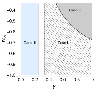
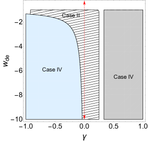
Figure 1: The allowed values for DE equation of state and Rastall parameters, subject to the conditions given in cases I-IV. The red dashed arrow corresponds to $\gamma=0$. The white region is not allowed for the model parameters.

IV.2 Dark Energy Dominated era

In order to study the effects of DE perturbations on the evolution of DM perturbations, we consider Eqs. (22) and (23) in DE dominated period. Let us begin with Eq. (III) which can be put into the following form

$$\ddot{a}=-\frac{aH^{2}}{2(6\gamma-1)}\Big{[}(6\gamma-1)(\Omega_{\rm m}+\Omega_{\rm de})+3(2\gamma-1)w_{\rm de}\Omega_{\rm de}\Big{]}.$$ (34)

Now, considering the following transformations for derivatives

$$\dot{\delta}=aH\delta^{\prime},~{}~{}~{}~{}~{}~{}~{}~{}~{}~{}\ddot{\delta}=\ddot{a}\delta^{\prime}+a^{2}H^{2}\delta^{\prime\prime},$$ (35)

together with using Eq. (34) we can re-express Eqs. (22) and (23) in terms of scale factor derivatives as

$$a^{2}\delta_{\rm m}^{\prime\prime}+ab_{0}\delta_{\rm m}^{\prime}-b_{1}\delta_{\rm m}=b_{2}\delta_{\rm de},$$ (36)

$$a^{2}\delta_{\rm de}^{\prime\prime}+ab_{0}\delta_{\rm de}^{\prime}-b_{4}\delta_{\rm de}=b_{3}\delta_{\rm m},$$ (37)

where

$$b_{0} = 2-\frac{1}{2}\left[\Omega_{\rm m}+\left(1+\frac{3(2\gamma-1)}{6\gamma-1}w_{\rm de}\right)\Omega_{\rm de}\right],$$

$$b_{1} = \frac{3(4\gamma-1)}{2(3\gamma-1)}\Omega_{\rm m},$$

$$b_{2} = \frac{3(4\gamma-1)\Big{(}3(2\gamma-1)w_{\rm de}+6\gamma-1\Big{)}}{2(3\gamma-1)(6\gamma-1)}\Omega_{\rm de},$$

$$b_{3} = \frac{3(1+w_{\rm de})(4\gamma-1)}{2\left(3\gamma(1+w_{\rm de})-1\right)}\Omega_{\rm m},$$

$$b_{4} = \frac{(1+w_{\rm de})(3\gamma-1)b_{2}}{3\gamma(1+w_{\rm de})-1}.$$

The system of differential equations (36) and (37) admits the following solutions for DM and DE perturbations as

$$\delta_{{\rm m}}(a) = {\sf C}_{5}a^{-\frac{1}{2}(b_{0}+B-1)}+{\sf C}_{6}a^{\frac{1}{2}(B-b_{0}+1)}$$ (39)

$$+ {\sf C}_{7}a^{-\frac{1}{2}(b_{0}+B_{1}-1)}+{\sf C}_{8}a^{\frac{1}{2}(B_{1}-b_{0}+1)},$$

$$\delta_{{\rm de}}(a) = \frac{1}{2b_{2}}\Big{[}{\sf C}_{5}Aa^{-\frac{1}{2}(b_{0}+B-1)}+{\sf C}_{6}Aa^{\frac{1}{2}(B-b_{0}+1)}$$

$$+ {\sf C}_{7}A_{1}a^{-\frac{1}{2}(b_{0}+B_{1}-1)}+{\sf C}_{8}A_{1}a^{\frac{1}{2}(B_{1}-b_{0}+1)}\Big{]},$$

where

$$B\!\!\! = \!\!\!\Big{[}b_{0}^{2}-2\sqrt{(b_{1}-b_{4})^{2}+4b_{2}b_{3}}$$

$$- 2b_{0}+2b_{1}+2b_{4}+1\Big{]}^{\frac{1}{2}},$$

$$B_{1}\!\!\! = \!\!\!\Big{[}b_{0}^{2}+2\sqrt{(b_{1}-b_{4})^{2}+4b_{2}b_{3}}$$

$$- 2b_{0}+2b_{1}+2b_{4}+1\Big{]}^{\frac{1}{2}},$$

$$A\!\!\! = \!\!\!b_{4}-\sqrt{(b_{1}-b_{4})^{2}+4b_{2}b_{3}}-b_{1},$$

$$A_{1}\!\!\! = \!\!\!b_{4}+\sqrt{(b_{1}-b_{4})^{2}+4b_{2}b_{3}}-b_{1}.$$ (41)

Note that in the limit of $\gamma\rightarrow 0$ we have

$$b_{0}\rightarrow 2-\frac{1}{2}\Omega_{\rm m}-\frac{1}{2}(1+3w_{\rm de})\Omega_{\rm de},$$

$$b_{1}\rightarrow\frac{3}{2}\Omega_{\rm m},~{}~{}~{}b_{2}\rightarrow\frac{3}{2}(1+3w_{\rm de})\Omega_{\rm de},$$

$$b_{3}\rightarrow\frac{3}{2}(1+w_{\rm de})\Omega_{\rm m},~{}~{}b_{4}\rightarrow\frac{3}{2}(1+w_{\rm de})(1+3w_{\rm de})\Omega_{\rm de}.$$

The unknown constants ${\sf C}_{5}-{\sf C}_{8}$ can be determined using the adiabatic initial conditions abramo2007 ; abramo2009

$$\frac{d\delta_{{\rm m}}}{dz}\Big{|}_{z=z_{i}}\!\!\! = -\frac{\alpha_{2}\delta_{\rm m}(z_{i})}{1+z_{i}},~{}~{}\frac{d\delta_{{\rm de}}}{dz}\Big{|}_{z=z_{i}}\!\!\!=-\frac{\alpha_{2}\xi\delta_{\rm m}(z_{i})}{1+z_{i}},$$

$$~{}~{}~{}\delta_{{\rm de}}(z_{i}) = \xi\delta_{{\rm m}}(z_{i}),$$ (43)

whence we finally obtain solutions (39) and (LABEL:deltadesolution) in terms of redshift $1+z=a^{-1}$, as

$$\delta_{{\rm m}}(z) = \frac{(1+z_{i})^{2(1-b_{0})}\delta_{{\rm m}}(z_{i})}{BB_{1}(A_{1}-A)}\Bigg{[}B_{1}(2\xi b_{2}-A_{1})\times$$ (44)

$$\!\!\!\!\!\!\!\!\!\!\!\!\Bigg{(}q_{1}\frac{(1+z)^{\frac{1}{2}(b_{0}+B-1)}}{(1+z_{i})^{\frac{1}{2}(B-3b_{0}+3)}}-q_{0}\frac{(1+z)^{\frac{1}{2}(b_{0}-B-1)}}{(1+z_{i})^{-\frac{1}{2}(B+3b_{0}-3)}}\Bigg{)}$$

$$+ q_{2}B(2\xi b_{2}-A)\frac{(1+z)^{\frac{1}{2}(b_{0}-B_{1}-1)}}{(1+z_{i})^{-\frac{1}{2}(B_{1}+3b_{0}-3)}}$$

$$- q_{3}B(2\xi b_{2}-A)\frac{(1+z)^{\frac{1}{2}(b_{0}+B_{1}-1)}}{(1+z_{i})^{\frac{1}{2}(B_{1}-3b_{0}+3)}}\Bigg{]},$$

$$\delta_{{\rm de}}(z) = \frac{(1+z_{i})^{2(1-b_{0})}\delta_{{\rm m}}(z_{i})}{BB_{1}b_{2}(A_{1}-A)}\Bigg{[}AB_{1}\left(\xi b_{2}-\frac{A_{1}}{2}\right)\times$$ (45)

$$\!\!\!\!\!\!\!\!\!\!\!\!\Bigg{(}q_{1}\frac{(1+z)^{\frac{1}{2}(b_{0}+B-1)}}{(1+z_{i})^{\frac{1}{2}(B-3b_{0}+3)}}-q_{0}\frac{(1+z)^{\frac{1}{2}(b_{0}-B-1)}}{(1+z_{i})^{-\frac{1}{2}(B+3b_{0}-3)}}\Bigg{)}$$

$$+ \frac{1}{2}q_{2}A_{1}B(2\xi b_{2}-A)\frac{(1+z)^{\frac{1}{2}(b_{0}-B_{1}-1)}}{(1+z_{i})^{-\frac{1}{2}(B_{1}+3b_{0}-3)}}$$

$$- \frac{1}{2}q_{3}A_{1}B(2\xi b_{2}-A)\frac{(1+z)^{\frac{1}{2}(b_{0}+B_{1}-1)}}{(1+z_{i})^{\frac{1}{2}(B_{1}-3b_{0}+3)}}\Bigg{]},$$

where

$$q_{0} = \alpha_{2}+\frac{1}{2}\left(b_{0}+B-1\right),~{}~{}q_{1}=\alpha_{2}+\frac{1}{2}\left(b_{0}-B-1\right),$$

$$q_{2} = \alpha_{2}+\frac{1}{2}\left(b_{0}+B_{1}-1\right),~{}~{}q_{3}=\alpha_{2}+\frac{1}{2}\left(b_{0}-B_{1}-1\right).$$

We can also integrate Eq. (36) for $\delta_{{\rm de}}=0$, in order to obtain the behavior of matter perturbations in the absence of DE perturbations. By doing so we get

$$\tilde{\delta}_{\rm m}(z) = \frac{\delta_{{\rm m}}^{\rm i}}{b_{0}-2q_{4}-1}\Bigg{[}(\alpha_{2}+b_{0}-q_{4}-1)\left(\frac{1+z}{1+z_{i}}\right)^{q_{4}}$$ (47)

$$- (\alpha_{2}+q_{4})\left(\frac{1+z}{1+z_{i}}\right)^{b_{0}-q_{4}-1}\Bigg{]},$$

where

$$q_{4}=\frac{1}{2}\left[b_{0}-\sqrt{b_{0}^{2}-2b_{0}+4b_{1}+1}-1\right],$$ (48)

and use has been made of the initial conditions given in Eq. (IV.2). The obtained expressions (44), (45) and (47) provide a wide class of solutions for density perturbations, depending on the Rastall parameter and EoS for DE. Firstly, from Eq. (36) we realize that DE perturbations can act as a source for matter perturbations in such a way that an overdensity in DE component could reduce ($b_{2}<0$) or enhance ($b_{2}>0$) matter perturbations. Figure (2) shows the space parameter constructed out of the pair $(\gamma,w_{\rm de})$ where the allowed regions for positive (shaded region) and negative (gray region) values of $b_{2}$ coefficient are plotted. Interestingly we observe that not always a DE overdensity decreases matter clustering and indeed, for certain values of $(\gamma,w_{\rm de})$ parameters we could have matter clustering for $w_{\rm de}<-1/3$. Such a scenario occurs for the shaded region confined between the blue arrow and the curves CD and EF. Moreover, an underdensity in DE perturbations does not necessarily lead to an overdensity in matter component, and instead, can provide both overdense ($b_{2}<0$) and underdense ($b_{2}>0$) regions of matter distribution. We also note that for all the points lying on the red arrow ($\gamma=0$), a DE overdensity decreases matter clustering for $w_{\rm de}<-1/3$ and vice versa. This is indeed the GR limit of the theory. In Fig. (3) we have plotted for the behavior of density contrasts against the redshift. We therefore observe that an underdensity in DE component (dashed curve within the upper panel) would enhance the evolution of matter component (solid curve) so that matter perturbations can grow even more than the case in which DE perturbations are absent (dot-dashed curve). It is also seen that the DE perturbations proceed towards formation of void. The lower panel presents the same scenario for which an overdensity occurs in DE component and consequently DE structures can also form during the evolution of perturbations. We note that the initial stages of structure formation can be adequately investigated within the linear approximation since the density contrast is small enough to neglect the quadratic terms within the system. However, as time goes by, the density contrast grows and consequently non-linear terms would play a major role in the amplitude of perturbations and the fate of the collapse process. This is the subject of the next section.

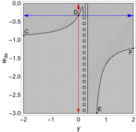
Figure 2: The allowed values for DE equation of state and Rastall parameters for which $b_{2}>0$ (shaded region) and $b_{2}<0$ (gray region). The red and blue arrows represent $\gamma=0$ and $w_{\rm de}=-1/3$ limits, respectively. The white region is not allowed for the model parameters.

Figure 3: Evolution of density contrasts $\delta_{{\rm m}}$ (solid curve), $\delta_{{\rm de}}$ (dashed curve) and $\tilde{\delta}_{{\rm m}}$ (dot-dashed curve) for $\gamma=-0.263$ and $w_{\rm de}=-1.11$ (upper panel) and $\gamma=-0.975$ and $w_{\rm de}=-0.68$ (lower panel). For upper and lower panels, we have chosen the pair $(\gamma,w_{\rm de})$ from gray and shaded regions of Fig. (2), respectively. For density parameters we have set $\Omega_{\rm de}=1-\Omega_{\rm m}=3/4.$

V Non-linear regime with varying $w_{\rm de}$

When considering the non-linear regime, things get slightly more complicated. Our aim is again to determine the density contrast, however, now we take into account the nonlinear terms within equations (19) and (III). By doing so, these equations for a varying DE state parameter then read

$$a^{2}\delta^{\prime\prime}_{{\rm m}} + ab_{0}\delta^{\prime}_{{\rm m}}-b_{1}(1+\delta_{{\rm m}})\delta_{{\rm m}}-b_{2}(1+\delta_{{\rm m}})\delta_{{\rm de}}$$ (49)

$$- a^{2}b_{5}\frac{\delta_{{\rm m}}^{\prime 2}}{1+\delta_{{\rm m}}}=0,$$

$$a^{2}\delta_{{\rm de}}^{\prime\prime} + ab_{0}\delta_{{\rm de}}^{\prime}-b_{3}(1+\delta_{{\rm de}})\delta_{{\rm m}}-b_{4}(1+\delta_{\rm de})\delta_{\rm de}$$

$$+ \frac{a^{2}\delta_{\rm de}^{\prime}w_{\rm de}^{\prime}}{(1+w_{\rm de})(3\gamma(1+w_{\rm de})-1)}-a^{2}b_{6}\frac{\delta_{\rm de}^{\prime 2}}{1+\delta_{\rm de}}=0,$$

where

$$b_{5}=\frac{15\gamma-4}{3(4\gamma-1)},~{}~{}b_{6}=\frac{3(1+w_{\rm de})(5\gamma-1)-1}{3(1+w_{\rm de})(4\gamma-1)}.$$ (51)

The above equations can be re-expressed in terms of the redshift using the following relations

$$\delta^{\prime} = -(1+z)^{2}\frac{d\delta}{dz},~{}w_{\rm de}^{\prime}=-(1+z)^{2}\frac{dw_{\rm de}}{dz}$$

$$\delta^{\prime\prime} = -(1+z)^{4}\frac{d^{2}\delta}{dz^{2}}+2(1+z)^{3}\frac{d\delta}{dz}.$$ (52)

Now if we take the following parametrization for DE state parameter eosdepar

$$w_{\rm de}(z)=w_{0}+w_{1}\frac{z}{1+z},$$ (53)

we can solve Eqs. (49) and (V) using numerical methods. The constants $w_{0}$ and $w_{1}$ can be chosen so that they are consistent with observational constraints w0w1constraints . As we expect the numerical solution for non-linear regime is different and depends crucially on the model parameters and initial data. We choose the initial density contrast for matter component to be a finite value at $z=2$. Therefore, the formation of matter structures commences at this redshift and evolves, along with the evolution of DE perturbations, until the present time ($z=0$). We find that in response to non-linear perturbations in DE, matter perturbations grow at a faster rate and reach a bigger amplitude than expected in linear regime. In Fig. (4) we have plotted the evolution of DM perturbations in the presence and absence of DE perturbations within upper and lower panels, respectively. For $\gamma=0$ (black solid curve), the DM density contrast grows monotonically and reaches a finite value at the present time, while for negative values of Rastall parameter, the matter perturbations grow faster so that DM structures may form before reaching the present epoch. For positive values of Rastall parameter (dashed and dot-dashed curves) we observe even more a rate of growth in matter perturbations in such a way that massive objects such as super-clusters can be born within the Universe. As we observe in the lower panel, matter perturbations start to grow from their initial values and diverge as we reach the present time. However, the rate of growth in density contrast for $\gamma=0$ (black solid curve) is lesser than the case in which the Rastall parameter is nonzero. Hence, in comparison to GR, we could have massive structures that form faster in Rastall gravity. We also observe that the overall growth rate of matter perturbations in the linear regime (long dashed and long dot-dashed curves) is much slower than the non-linear one. Though, at initial stages of the collapse process, the evolution of density contrasts in both linear and non-linear regimes coincide, non-linear perturbations start detaching from the linear ones as the collapse proceeds to lower redshifts. We also note that as numerical simulations are approximate solutions of the governing equations, differences between numerical solutions and exact ones are expected. The difference is the numerical error. Figure (5) shows the numerical error associated with the solution of the system (49) and (V) where we observe that the numerical solution presented in Fig. (4) satisfies these equations with the accuracy of the order of $10^{-8}$ or less.

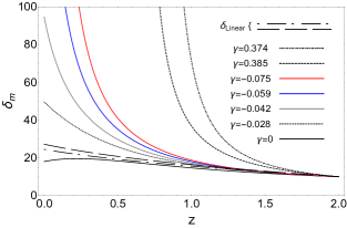
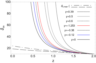
Figure 4: Evolution of the matter perturbations with (upper panel) and without (lower panel) taking into account the DE perturbations. The initial value of matter density contrast has been chosen as $\delta_{\rm m}(z=2)=10$. For parametrization of DE equation of state we have set $w_{0}=-0.75$ and $w_{1}=0.4$. For density parameters we have set $\Omega_{\rm de}=1-\Omega_{\rm m}=3/4.$ The long dashed and long dot-dashed curves represent the evolution of matter perturbations in linear regime for the same values of model parameters as chosen in Fig.(3).

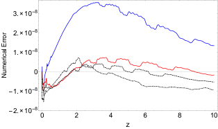
Figure 5: Numerical error associated to the numerical solution given in Fig.(4). The blue and red curves have been plotted for $\gamma=-0.059$ and $\gamma=-0.075$ and the dashed and dot-dashed curves have been plotted for $\gamma=0.385$ and $\gamma=0.374$, respectively.

VI Concluding Remarks

In the present work we studied the evolution of DM and DE perturbations in the context of Rastall theory. In order to simplify the analysis, we restricted ourselves to spherically symmetric perturbations. Thus, for a spherically symmetric top-hat collapse, we investigated dynamics of density contrast for dark components in both linear and non-linear regimes. In the linear regime, we observed that the Rastall parameter could play an important role in the growth of DM perturbations. Moreover, DM perturbations could in turn provide a setting for enhancing or decreasing the growth of DE perturbations. In DE dominated era, we obtained exact solutions for the set of differential equations that govern the dynamics of density contrasts of DE and DM. We found that DE perturbations could increase the rate of growth of DM perturbations so that they grow even faster than the case in which DE perturbations are absent. Numerical solutions to perturbation equations in non-linear regime show a different scenario. Matter perturbations could grow more rapidly compared with the linear case so that structures which collapse in this manner could be denser than those of linear regime. Hence, the collapse process in non-linear regime could lead to the formation of super clusters of DM. We further note that depending on the values and signs of the pair $(\gamma,w_{\rm de})$ other types of solutions can be obtained, in which, DE and DM perturbations experience oscillations with different frequencies and amplitudes. One then can interpret such a behavior as the ability of spacetime and matter fields to couple to each other in non-minimal way, that the representative of which is the Rastall parameter. We therefore observe that the DE and DM perturbations in Rastall theory could lead to different fates in comparison to GR. From observational viewpoint, Batista et al. batista2013 used the data of type Ia supernovae to constrain the Rastall parameter. Their results show that the credible regions in $(\gamma,w_{\rm de})$ plane allow the $\gamma$ parameter to extend to very small and very large values. In this regard, the results of batista2013 confirm the allowed values of $(\gamma,w_{\rm de})$ parameters we obtained in Figs. (1) and (2). Other observational constraints on Rastall theory have been reported in the literature, for example, the Bayesian method carried out to fit the rotation curves of 16 low surface brightness spiral galaxies, showed that the Rastall parameter is of order $10^{-1}$ Meirong2020 , which is consistent with the strong lensing estimation mnras2019ras . Also, the study of interiors of neutron stars with realistic EoS has reported an astrophysical constraint on this parameter to be of order $10^{-2}$ oliveira2015 . Despite the successes of Rastall theory in describing cosmological as well as astrophysical scenarios, providing a conclusive constraint on Rastall parameter is still under debate and the model needs to be meticulously confronted with the observational data. From this point of view, though in the present work we did not perform a comprehensive and thorough study of the observational aspects of Rastall theory, we tried to shed some light on the non-equivalence of Rastall gravity and GR. A more profound analysis along this line is a subject of our future research work to further put to the test the viability of Rastall gravitation theory in comparison to GR with the help of upcoming precise observational data.

As the final remarks, we would like to mention that, though the SC model is an approximation to more realistic collapse scenarios, it provides a suitable framework to investigate the time scale of halo collapse and has proven to be a very useful tool in developing approximate statistical models for the formation and evolution of halos and their abundances. Moreover, this model is very successful in reproducing results of N-body simulations when mass is combined with the function formalism DPopolo ; DPopolo1 , either in usual minimally coupled DE models Pace2010 or in non-minimally coupled DE models Pace2014 . However, it is important to extend the basic formalism of SC model in order to incorporate additional terms and make it more realistic. Work along this line has been done e.g., by relaxing the assumption of spherical symmetry Hoffman1986 ; Hoffman1989 ; Zaroubi1993 , introducing radial motions and angular momentum Ryden1987 ; DPopolo2 ; Lentz2016 ; Cupani2011 , studying the effects of DE inhomogeneities nunes2006 ; abramo2009 ; manera2006 ; Pace2013 ; Pereira2010 and shear and rotation Reischke2018 ; DelPolo2018 ; DelPolo2020 ; FPace2014 ; DPopolo3 , see also DelPopoloAA ; Daichi2016 ; Pace2017 and references therein. In this regard, extending the results of the present work to include more realistic scenarios could provide us a guideline for better understanding the mutual matter-geometry interaction and possibly its footprints in the formation of cosmic structures.

References

- (1) P. Rastall, Phys. Rev. D 6, 3357 (1972).
- (2) P. Rastall, Can. J. Phys. 54, 66 (1976).
- (3) A. S. Al-Rawaf and M. O. Taha, Phys. Lett. B 366, 69 (1996).
- (4) A. S. AI-Rawaf and M. O. Taha, Gen. Relative. Gravit., 28, 935 (1996).
- (5) H. Moradpour, Y. Heydarzade, F. Darabi and Ines G. Salako, Eur. Phys. J. C 77, 259 (2017).
- (6) G. W. Gibbons and S.W. Hawking, Phys. Rev. D 15, 2738 (1977).
- (7) N. D. Birrell and P. C. W. Davies, Quantum Fields in Curved Space (Cambridge University Press, Cambridge, 1982).
- (8) J. C. Fabris, O. F. Piattella, D. C. Rodrigues1 and M. H. Daouda, AIP Conf. Proc. 50, 1647 (2015).
- (9) H. Shabani and A. H. Ziaie, Int. J. Mod. Phys. A 33, 1850050 (2018).
- (10) H. Shabani and M. Farhoudi, Phys. Rev. D 88, 044048 (2013).
- (11) H. Shabani and M. Farhoudi, Phys. Rev. D 90, 044031 (2014).
- (12) R. A. Bertlemann, Anomalies in quantum field theory, (Oxford university press, Oxford 1996).
- (13) J. C. Fabris and G. T. Marques, Eur. Phys. J. C 72, 2214 (2012).
- (14) C. E. M. Batista, J. C. Fabris and M. Hamani Daouda, Nuovo Cim. B 125, 957 (2010).
- (15) M. Capone, V. F. Cardone and M. L. Ruggiero, Nuovo Cim. B 125, 1133 (2010).
- (16) J. C. Fabris, T. C. C. Guio, M. Hamani Daouda and O. F. Piattella, Grav. Cosmol. 17, 259 (2011).
- (17) C. E. M. Batista, M. H. Daouda, J. C. Fabris, O. F. Piattella and D. C. Rodrigues, Phys. Rev. D 85, 084008 (2012).
- (18) C. E. M. Batista, J. C. Fabris, O. F. Piattella, A. M. Velasquez-Toribio, Eur. Phys. J. C 73, 2425 (2013).
- (19) G. F. Silva, O. F. Piattella, J. C. Fabris, L. Casarini and T. O. Barbosa, Grav. Cosmol. 19, 156 (2013).
- (20) H. Moradpour, Phys. Lett. B 757, 187 (2016).
- (21) H. Moradpour, A. Bonilla, E. M. C. Abreu, and J. A. Neto, Phys. Rev. D 96, 123504 (2017).
- (22) A. F. Santos and S. C. Ulhoa, Mod. Phys. Lett. A 30, 1550039 (2015).
- (23) T. R. P. Caramês et. al., EPJC 74, 3145 (2014).
- (24) I. G. Salako, M. J. S. Houndjo and A. Jawad, Int. J. Mod. Phys. D 25, 1650076 (2016).
- (25) A. M. Oliveira, H. E. S. Velten, J. C. Fabris and L. Casarini, Phys. Rev. D 92, 044020 (2015).
- (26) A. M. Oliveira, H. E. S. Velten and J. C. Fabris, Phys. Rev. D 93, 124020 (2016).
- (27) H. Moradpour and I. G. Salako, Adv. High Energy Phys. 2016, 3492796 (2016).
- (28) K. A. Bronnikov, J. C. Fabris, O. F. Piattella, E. C. Santos, Gen. Rel. Grav. 48, 162 (2016).
- (29) Y. Heydarzade, H. Moradpour and F. Darabi, Can. J. Phys. 95, 1253 (2017).
- (30) K. Lin, W.-L. Qian, Chi. Phys. C 43, 083106 (2019).
- (31) V. Majernik and L. Richterek, arxiv: gr-qc/0610070.
- (32) M. Visser, Phys. Let. B 782, 83 (2018).
- (33) F. Darabi, H. Moradpour, I. Licata, Y. Heydarzade and C. Corda, Eur. Phys. J. C 78, 25 (2018).
- (34) H. Moradpour, I. Licata, C. Corda and Ines G. Salako, Mod. Phys. Lett. A 33, 1950096 (2019).
- (35) H. Moradpour, Y. Heydarzade, C. Corda, A. H. Ziaie, S. Ghaffari, Mod. Phys. Lett. A, 33, 1950304 (2019).
- (36) F.-F. Yuan and P. Huang, Class. Quant. Grav. 34, 077001 (2017).
- (37) H. Moradpour, C. Corda, I. Licata, arxiv: gen-ph/1711.01915.
- (38) H. Moradpour, N. Sadeghnezhad and S. H. Hendi, Can. J. Phys, 95, 1257 (2017).
- (39) I. P. Lobo, H. Moradpour, J. P. Morais Graça and I. G. Salako, Int. J. Mod. Phys. D 27, 1850069 (2018).
- (40) R. Kumar and S. G. Ghosh, Eur. Phys. J. C 78, 750 (2018).
- (41) K. Bamba, A. Jawad, S. Rafique and H. Moradpour, Eur. Phys. J. C 78, 986 (2018).
- (42) H. Moradpour and M. Valipour, Can. J. Phys. 98, 853 (2020).
- (43) S. Halder, S. Bhattacharya, S. Chakraborty, Mod. Phys. Lett. A 34, 1950095 (2019).
- (44) W. Khyllep and J. Dutta, Phys. Let. B 797, 134796 (2019).
- (45) R. Li, J. Wang, Z. Xu and X. Guo, MNRAS, 486, 2407 (2019).
- (46) A. M. Oliveira, H. E. S. Velten, J. C. Fabris, L. Casarini, Phys. Rev. D 92, 044020 (2015).
- (47) S. K. Maurya, F. Tello-Ortiz, Phys. Dark Univ. 29, 100577 (2020).
- (48) X.-C. Cai, Y.-G. Miao, Phys. Rev. D 101, 104023 (2020).
- (49) C. E., Mota, L. C. N. Santos, G. Grams, F. M. da Silva, D. P. Menezes, Phys. Rev. D 100, 024043 (2019).
- (50) I. P., Lobo, R. G. Martin, J. P. Morais Graça and H. Moradpour, Eur. Phys. J. Plus 135, 550 (2020).
- (51) J. Llibre, and C. Pantazi, Class. Quant. Grav. 37, 245010 (2020).
- (52) P. Xi, Q. Hu, G.-nan Zhuang, X.-zhou Li, Astrophys. Space Sci. 365, 163 (2020).
- (53) A. Singh and K. C. Mishra, Eur. Phys. J. Plus 135, 752 (2020).
- (54) G. Mustafa, and T.-C. Xia, Int. J. Mod. Phys. A, 35, 2050109 (2020).
- (55) A. H. Ziaie, H. Moradpour and H. Shabani, Eur. Phys. J. Plus, 135, 916 (2020).
- (56) G. Mustafa, S. Waheed, M. Zubair, T.-C., Xia, Chin. J. Phys., 65, 163 (2020).
- (57) H. L. Prihadi, M. F. A. R. Sakti, G. Hikmawan and F. P. Zen, Int. J. Mod. Phys. D 29, 2050021 (2020).
- (58) Z.-X. Yu, S.-L. Li and H. Wei, Nucl. Phys. B, 960, 115179 (2020).
- (59) A. H. Ziaie, Y. Tavakoli, Annalen Phys. 532, 2000064 (2020).
- (60) A. H. Ziaie, H. Moradpour, S. Ghaffari, Phys. Let. B 793, 276 (2019).
- (61) L. L. Smalley, J. Phys. A: Mathematical and General 16, 2179 (1983).
- (62) S. Hansraj, A. Banerjee and P. Channuie, Ann. Phys. 400, 320 (2019).
- (63) R. C. Tolman, Phys. Rev. 55, 364 (1939).
- (64) G. Abbas and M. R. Shahzad, Eur. Phys. J. A 54 (2018) 1434.
- (65) G. Abbas and M. R. Shahzad, Chinese Journal of Physics 63, 1 (2020).
- (66) D. Das, S. Dutta and S. Chakraborty, Eur. Phys. J. C 78, 810 (2018).
- (67) S. D. M. White and M. J. Rees, Mon. Not. R. Astron. Soc. 183, 341 (1978).
- (68) P. J. E. Peebles, Principles of Physical Cosmology (Princeton University Press, Princeton, NJ, 1993).
- (69) J. A. Peacock, Cosmological Physics (Cambridge University Press, Cambridge, UK, 1999).
- (70) L. R. Abramo, R. C. Batista, L. Liberato and R. Rosenfeld, JCAP 0711, 012 (2007).
- (71) N. J. Nunes, A. C. da Silva and N. Aghanim, Astron. Astrophys. 450 899 (2005).
- (72) L. Liberato and R. Rosenfeld, JCAP 07, 009 (2006).
- (73) N. J. Nunes and D. F. Mota, Mon. Not. R. Astron. Soc. 368, 751 (2006).
- (74) M. Manera and D. F. Mota, MNRAS, 371, 1373 (2006).
- (75) S. Dutta and I. Maor, Phys. Rev. D 75, 063507 (2007).
-
(76)
H. Kodama and M. Sasaki, Prog. Theor. Phys. Suppl. 78, 1 (1984);
L. Amendola and S. Tsujikawa, “Dark energy-Theory and Observations,” Cambridge University Press (2010). - (77) L. R. Abramo, R. C. Batista, L. Liberato and R. Rosenfeld, Phys. Rev. D 79, 023516 (2009).
- (78) T. Manna, F. Rahaman and M. Mondal, Mod. Phys. Lett. A 35, 2050034 (2020).
- (79) K. Lin and W.-Liang Qian, Eur. Phys. J. C, 80, 561 (2020).
- (80) K. A. Bronnikov, J. C. Fabris, O. F. Piattella, D. C. Rodrigues and E. C. Santos, Eur. Phys. J. C 77, 409 (2017).
- (81) J. E. Gunn and J. R. Gott, Astrophys. J., 176, 1 (1972).
- (82) O. Lahav, P. B. Lilje, J. R. Primack, and M. J. Rees, MNRAS, 251 128 (1991).
-
(83)
D. F. Mota and C. van de Bruck, Astron. Astrophys., 421, 71 (2004);
P. Creminelli, G. D’Amico, J. Norena, L. Senatore, and F. Vernizzi, JCAP, 1003, 027 (2010);
M. P. Rajvanshi and J. S. Bagla, JCAP, 1806, 018 (2018). - (84) S. Basilakos, M. Plionis, and J. Sola. Phys. Rev. D 82, 083512 (2010).
-
(85)
F. Schmidt, M. V. Lima, H. Oyaizu, and W. Hu, Phys. Rev. D 79, 083518 (2009);
A. Borisov, B. Jain, and P. Zhang, Phys. Rev. D 85, 063518 (2012);
M. Kopp, S. A. Appleby, I. Achitouv, and J. Weller, Phys. Rev. D 88, 084015 (2013)
D. Herrera, I. Waga, and S. E. Joras, Phys. Rev. D 95, 64029 (2017);
Ph. Brax, R. Rosenfeld, and D. A. Steer, JCAP, 1008, 033 (2010). -
(86)
S. Lee and K.-Wang Ng, JCAP, 2010, 028 2010;
R. C. Batista and V. Marra, JCAP, 1711, 048 (2017);
C.-C. Chang, W. Lee, and K.-Wang Ng, Phys. Dark Univ., 19, 12 (2018). -
(87)
S. Sapa, K. Karwan, and D. F. Mota, Phys. Rev. D, 98, 023528 (2018);
N. Wintergerst and V. Pettorino, Phys. Rev. D 82, 103516 (2010). - (88) T. Harko, F. S. N. Lobo, S. Nojiri and S. D. Odintsov, Phys. Rev. D 84, 024020 (2011).
- (89) T. Harko and F. S. N Lobo, Eur. Phys. J. C 70, 373 (2010).
- (90) T. Harko and F. S. N Lobo, Galaxies 2, 410 (2014).
- (91) W. A. G. De Moraes and A. F. Santos, Gen. Rel. Grav. 51, 167 (2019).
- (92) H. Shabani and A. H. Ziaie, Europhysics Letters 129, 20004 (2020).
- (93) J. J. Van Der Bij and H. Van Dam, Physica 116A, 307 (1982).
- (94) Diego Sáez-Gómez, Phys. Rev. D 93, 124040 (2016).
- (95) M. Shaposhnikov , D. Zenhäusern, Phys. Lett. B 671, 187 (2009).
- (96) A. M. Oliveira, H. E. S. Velten and J. C. Fabris, Phys. Rev. D 93, 124020 (2016).
- (97) M. Daouda, J. C. Fabris, A. M. Oliveira, F. Smirnov, H. E. S. Velten, Int. J. Mod. Phys. D 28, 1950175 (2019).
- (98) Ö. Akarsu, N. Katırcı, S. Kumar, R.l C. Nunes, B. Öztürk and S. Sharma Eur. Phys. J. C 80, 1050 (2020).
- (99) R. Ferraro, Einstein’s Space-Time: An Introduction to Special and General Relativity, Springer Science & Business Media, (2007).
- (100) M. Chevallier, D. Polarski, Int. J. Mod. Phys. D 10, 213 (2001).
-
(101)
Y. Wang and P. Mukherjee, Phys. Rev. D 76, 103533 (2007);
E. L. Wright, Astrophys. J. 664, 633 (2007). - (102) M. Tang, Z. Xu and J. Wang, Chinese Phys. C 44 085104 (2020).
- (103) A. Del Popolo, Astronomy Reports, 51, 169 (2007).
- (104) N. Hiotelis and A. Del Popolo, MNRAS, 436, 163 (2013).
- (105) F. Pace, J. C. Waizmann and M. Bartelmann, MNRAS, 406, 1865 (2010).
- (106) F. Pace, L. Moscardini, R. Crittenden, M. Bartelmann and V. Pettorino, MNRAS, 437, 547 (2014).
- (107) Y. Hoffman, ApJ, 308, 493 (1986).
- (108) Y. Hoffman, ApJ, 340, 69 (1989).
- (109) S. Zaroubi and Y. Hoffman, ApJ, 416, 410 (1993).
- (110) B. S. Ryden, J. E. Gunn, ApJ, 318, 15 (1987).
- (111) A. Del Popolo, Astronomy Reports, 63, 971 (2019).
- (112) E. W. Lentz, T. R. Quinn and L. J. Rosenberg, The Astrophysical Journal, 822, 89 (2016).
- (113) G. Cupani, M. Mezzetti and F. Mardirossian, MNRAS, 417, 2554 (2011).
- (114) R. C. Batista and F. Pace, JCAP 1306, (2013) 044.
- (115) T. S. Pereira, R. Rosenfeld and A. Sanoja, Europhys. Lett., 92, 39001 (2010).
- (116) R. Reischke, F. Pace, S. Meyer and B. M Schäfer, MNRAS, 473, 4558 (2018).
- (117) A. Del Popolo and X. Lee, Astronomy Reports, 62, 475 (2018).
- (118) A. Del Popolo, M. H. Chan and D. F. Mota, Phys. Rev. D, 101, 083505 (2020).
- (119) F. Pace, R. C. Batista and A. Del Popolo, MNRAS, 445, 648 (2014).
- (120) A. Del Popolo, F. Pace and J. A. S. Lima, MNRAS 430, 628 (2013).
- (121) A. Del Popolo, AA 454, 17 (2006).
- (122) D. Suto, T. Kitayama, K. Osato, S. Sasaki and Y. Suto, Pub. Astron. Soc. Japan, 68, 14 (2016).
- (123) F. Pace, S. Meyer and M. Bartelmann, JCAP 10 (2017) 040.