Concentration on the Boolean hypercube via pathwise stochastic analysis
Abstract
We develop a new technique for proving concentration inequalities which relate between the variance and influences of Boolean functions. Using this technique, we
-
1.
Settle a conjecture of Talagrand [Tal97], proving that
where is the number of edges at along which changes its value, and is the influence of the -th coordinate.
-
2.
Strengthen several classical inequalities concerning the influences of a Boolean function, showing that near-maximizers must have large vertex boundaries. An inequality due to Talagrand states that for a Boolean function , . We give a lower bound for the size of the vertex boundary of functions saturating this inequality. As a corollary, we show that for sets that satisfy the edge-isoperimetric inequality or the Kahn-Kalai-Linial inequality up to a constant, a constant proportion of the mass is in the inner vertex boundary.
-
3.
Improve a quantitative relation between influences and noise stability given by Keller and Kindler.
Our proofs rely on techniques based on stochastic calculus, and bypass the use of hypercontractivity common to previous proofs.
1 Introduction
1.1 Background
The influence of a Boolean function in direction is defined as
where is the same as but with the -th bit flipped, and is the uniform measure on the discrete hypercube . The expectation and variance of a function are given by
The Poincaré inequality gives an immediate relation between the aforementioned quantities, namely,
| (1) |
The total influence on the right hand side is equal to the number of edges of the hypercube which separate and . It can therefore be seen as a type of surface-area of .
The inequality (1) in fact holds for any function (for a suitably defined influence), and it is natural to ask whether it can be improved when Boolean functions are considered. A corollary of the breakthrough paper by Kahn, Kalai and Linial (KKL) [KKL88] shows that this inequality can be strengthened logarithmically: There exists a universal constant such that
| (2) |
(The above formulation does not appear explicitly in [KKL88], but follows easily from their methods).
The KKL inequality is tight for the Tribes function, but is off by a factor of for the majority function, whose influences are all of order , suggesting that the total influence may not be the right notion of surface-area for all Boolean functions. In [Tal93, Theorem 1.1], Talagrand showed that
| (3) |
where is the sensitivity of at point . The value can be seen as another type of surface-area of the function . A sharp tightening of this inequality was given by Bobkov [Bob97]; his inequality gives an elementary proof of the isoperimetric inequality on Gaussian space. Inequality (3) is tight for linear-threshold functions such as majority, but not for Tribes. Thus, neither inequality implies the other. This raises the following question:
Question 1.
As a step in this direction, Talagrand conjectured in [Tal97] that (3) can be strengthened, and that there exists a constant such that
| (4) |
Talagrand showed that there exists an and a constant such that
but his proof did not yield the conjectured , and it falls short of recovering the logarithmic improvement in the KKL inequality.
Another notion of surface-area is the vertex boundary of , defined as
It is the disjoint union of the inner vertex boundary,
and the outer vertex boundary,
The Cauchy-Schwartz inequality implies that , so the above conjecture strengthens the KKL result in the regime (see below Theorem 4 for a calculation).
The inequality (2) was further generalized in another direction by Talagrand [Tal94], who proved the following:
Theorem 2.
There exists an absolute constant such that for every ,
| (5) |
It is known that this inequality is sharp in the sense that for any sequence of influences, there exist examples which saturate it [KLS+15].
Inequalities such as (2), (4) and (5), in conjunction with concentration of influence [Fri98] and sharp threshold properties [Fri99], have been widely utilized across many subfields of mathematics and computer science, including learning theory [OS07], metric embeddings [KR09], first passage percolation [BKS03], classical and quantum communication complexity [Raz95, GKK+09], and hardness of approximation [DS05]; and also in social network dynamics [MNT14] and statistical physics [BDC12]. For a general survey, see [KS06].
1.2 Our results
In this paper, we develop a new approach towards the proofs of the aforementioned inequalities. Our proofs are based on pathwise analysis, which bypasses the use of hypercontractivity, and in fact uses classical Boolean Fourier-analysis only sparingly. Using these techniques, we first to show that Talagrand’s conjecture holds true:
Theorem 3.
There exists an absolute constant such that for all ,
In fact, we prove a stronger theorem, of which Theorem 3 is an immediate corollary:
Theorem 4.
There exists an absolute constant such that the following holds. For all , there exists a function with so that for all ,
| (6) |
The above inequality with implies both the KKL inequality in full generality and a new lower bound on total influences in the spirit of the isoperimetric inequality. By the Cauchy-Schwartz inequality,
and plugging this into (6), we get
| (7) |
From this equation we can proceed in two directions:
Theorem 4 KKL
Denoting , the above display yields
Consider now two cases: If , we immediately get from the above display that . And if , we have
(for , otherwise there is nothing to prove), again yielding .
Hierarchically, the relation between the Poincaré inequality, KKL, Talagrand’s theorem and Theorem 4 may be summarized as in Figure 1.
Theorem 4 Stability of the Isoperimetric inequality
Assume that and let be the support of , so that . The edge-isoperimetric inequality [Har76, section 3] states that
| (8) |
with equality if and only if is a subcube. Suppose that saturates the isoperimetric inequality up to a constant, i.e
for some constant . Since , this gives
| (9) |
Suppose also that is monotone; then , and from equations (7) and (9) we get that
In particular, the two denominators are within a constant factor of each other:
implying that the Fourier mass on the first level is proportional to a power of the variance.
Next, we reprove Theorem 2 using stochastic techniques, and provide a strengthening which can be thought of as a stability version of this bound in terms of the vertex boundary of : If near-equality is attained in equation (5), then both the inner and outer vertex boundaries of are large. The theorem reads,
Theorem 5.
Let , and denote . There exists an absolute constant such that
Theorem 5 can be readily applied to two related functional inequalities - the isoperimetric inequality and the KKL inequality - showing that when either of the inequalities are tight up to a constant, the function must have a large vertex boundary.
The Isoperimetric inequality and vertex boundary
It is natural to ask about the robustness of the isoperimetric inequality: Is it true that if near-equality is attained in (8), then is close to a subcube in some sense? This question was answered in [Ell11] for sets which are -close to satisfying the inequality. Conjectures concerning sets for which the inequality is tight only up to a constant multiplicative factor can be found in [KK07]. We make a step in this direction by giving the first bound which is meaningful when the function is -close to satisfying the inequality (8), showing that in that case, a constant proportion of the set is in its inner vertex boundary (whereas for the extremizers, the vertex boundary is the entire set ).
Corollary 6.
Let Then there exists a constant depending only on such that
The KKL inequality and vertex boundary
In its original formulation, the KKL theorem [KKL88, Theorem 3.1], which follows immediately from (2), states that a Boolean function must have a variable with a relatively large influence: There exists an absolute constant such that for every , there exists an index with
Our second corollary states that if all influences are of the order , then the function must have a large (inner and outer) vertex boundary.
Corollary 7.
Suppose that for some , we have for all . Then there exists a constant depending only on such that
Proof.
Finally, we improve an inequality by Keller and Kindler [KK13]. Let be the noise stability of , i.e
where is a random vector whose -th coordinate is equal to with probability and to a uniformly random bit with probability .
Theorem 8.
There exists universal constants such that
| (10) |
The bound proved in [KK13] is the same but with the term is replaced by a constant; thus our result becomes stronger when This theorem is used in the proof of Theorem 2. The relation between influences and noise sensitivity was first established in [BKS99], where a qualitative bound of the same nature is proven.
1.3 Proof outline
The core of our proofs is the construction of a martingale which satisfies and (Proposition 11).
Since is uniform on the hypercube, the expected value and variance of can be obtained by and , where the expectations in the right hand sides are over the randomness of the process . Similarly, the influence of the -th bit is given by , where is the partial derivative of in direction , and is given by .
The strength of the stochastic process approach stems from the fact that the behavior of can be understood by an analysis of the processes , and for times smaller than . Indeed, there is a natural way to extend the domain of a Boolean function to the continuous hypercube so that the processes and become martingales. The variance of can then be expressed as
(Lemma 13 and Corollary 14). Bounding the variance is then a matter of bounding the integral , and for this we can utilize tools from real analysis and stochastic processes. Specifically, two well-known inequalities - called the Level-1 and Level-2 inequalities - give us bounds on the speed with which both the individual processes and their collective sum are moving in terms of their current value. In the Gaussian setting, somewhat similar ideas of using level inequalities appear in [Eld15].
This points to a significant conceptual difference between existing techniques that use the hypercontractivity of the heat operator and our technique: Whereas the former proofs start from the function and analyze the way that it changes by applying the heat semigroup, which corresponds to going backwards in the time , our analysis goes forward in time. We may think of the process as a way to sample from via a continuous filtration, where we add “infinitesimal bits of randomness” as time progresses. The analysis starts from and considers the way that the martingales evolve as we refine our filtration, or in other words, add more randomness. On a first glance this difference may seem to be only pedagogical, but the strength of our approach is that the pathwise analysis equips us with new tools, such as using stopping times and the optional stopping theorem, and conditioning on the past.
Towards proving Talagrand’s conjecture, we use the Level-2 inequality (Lemma 10) to bound by a time-dependent power of the sum of squares of influences . Ideologically, when this sum is small, this roughly implies that the process makes most of its movement very close to time ; this is in fact the essence of Theorem 8. This can then be used to show that most of the quadratic variation of comes from paths in which there is a time such that is larger than (Proposition 19). However, the quadratic variation is itself large with probability that is directly proportional to the variance (Proposition 20). This is one of the steps where the pathwise analysis is crucially used; without it, we would have only known that the quadratic variation is large in expectation, which would not eliminate the possibility that the entire contribution to the variance is made on an event of negligible probability. Since is a submartingale, if there was ever a time when is large, then in expectation it continues to be large. Thus is larger than , giving the original Talagrand’s conjecture (Theorem 3) when . With additional care, it can be shown that itself is large at some time before the gradient was large, which gives the strengthened result (Theorem 4).
This is a good place to point out an analogy between our technique and the one demonstrated by Barthe and Maurey [BM00], who give a stochastic proof of Bobkov’s extension of inequality (3). They use a stochastic argument in order to derive a one-dimensional inequality which implies Bobkov’s inequality via tensorization, and one of the central components in their proof is to establish that a certain process which is analogous to is a submartingale (this is based on ideas introduced in a paper by Capitaine, Hsu and Ledoux [CHL97]).
Similarly, for proving Theorem 2, we use the Level-1 inequality (Lemma 9) to bound each individual by a time-dependent power of the influence (Lemma 22). When the influences are small, this roughly implies that the martingale makes most of its movement very close to time . Theorem 2 then follows by plugging this bound into the integral (Proposition 23).
The proof of Theorem 5 is more involved, and utilizes the fact that is both a jump process and a martingale: For such processes, the variance of is then given by the sum of squares of jumps of up to time :
The technical core of the proof (Proposition 24 and Lemma 25) shows that if and differ only by a multiplicative constant, then with non-negligible probability the process must make a relatively large jump somewhere along the way. Roughly speaking, this is because if the process jumps at time , then the function also jumps, changing by a value of . If all the jumps are small, then the expression in the left hand side of the above display (which cares only about jumps) must be substantially smaller than the integral in the right hand side (which cares only about the size of the derivatives).
Now, when the process makes a large jump, it necessarily means that the magnitude of one of the partial derivatives is large. Since the process is also a martingale, if it is large at some point in time, then it continues to be large with relatively high probability. But at time , since is uniform on the hypercube, the only possibilities for the values of are , and . Thus, it is likely that . This exactly corresponds to the point being in the vertex boundary, showing that the vertex boundary is large. The distinction between the inner and outer vertex follows by similar arguments, using a symmetrification of (Proposition 26).
Acknowledgements
R.E. would like to thank Noam Lifshitz for useful discussions and in particular for pointing out the possible application to stability of the isoperimetric inequality. We are also thankful to Ramon Van Handel, Itai Benjamini and Gil Kalai for an enlightening discussion, and grateful for the comments from the anonymous STOC referees.
2 Preliminaries
Throughout the text, the letter stands for a positive universal constant, whose value may change from line to line.
2.1 Boolean functions
For a general introduction to Boolean functions, see [O’D14]; in what follows, we provide a brief overview of the required background and notation.
Every Boolean function may be uniquely written as a sum of monomials:
| (11) |
where , and the harmonic coefficients (also known as Fourier coefficients) are given by
| (12) |
Equation (11) may be used to extend a function’s domain from the discrete hypercube to real space . We call this the harmonic extension, and denote it also by . Under this notation, . In general, for , the harmonic extension is a convex combination of ’s values on all the points :
| (13) |
where .
The derivative of a function in direction is defined as
where has at coordinate , and is identical to at all other coordinates. The gradient is then defined as . A function is called monotone if whenever for all . Similar to the function , by abuse of notation will denote the harmonic extension of , and we will treat it as a function on .
A short calculation reveals the following properties of the derivative:
-
1.
The harmonic extension of the derivative is equal to the real-differentiable partial derivative of the harmonic extension of .
-
2.
For functions whose range is , the derivative takes values in , and the influence of the -th coordinate of is given by
(14) -
3.
For monotone functions, the derivative only takes values in , and the influence of the -th coordinate is then given by
(15)
In the definition of the Fourier coefficient in (12), the expectation is over the uniform measure . It is also possible to decompose a function into Fourier coefficients over a biased measure. This type of analysis will be used only in the proof of Theorem 8. A brief overview can be found in the appendix.
Finally, we’ll require two lemmas which effectively relate the weights of the Fourier coefficients at higher levels with those of lower ones; this translates to inequalities between the harmonic extension of a function and its derivatives. The first lemma is a direct application of the fact that is subgaussian; it essentially bounds the Fourier weights in the first level by a function of the weights at level zero:
Lemma 9 (Level-1 inequality).
There exists a constant so that the following holds. Let be the harmonic extension of a Boolean function, and let be such that for all . Then
| (16) |
The second lemma, whose original, uniform case is due to Talagrand [Tal96], essentially bounds the Fourier weights in the second level by those of the first. It is similar to [KK13, Lemma 6], but for real-valued functions.
Lemma 10 (Level-2 inequality).
There exists a continuous function so that the following holds. Let be the harmonic extension of a monotone function, and let be such that for all . Then
| (17) |
where is the Hessian of , and is the Hilbert-Schmidt norm of a matrix.
Remark.
In both lemmas, the requirement that for all is not crucial, and can be replaced by for all .
The proofs of both lemmas are found in the appendix.
2.2 Stochastic processes and quadratic variation
A Poisson point process with rate is an integer-valued process such that , and for every , the difference distributes as a Poisson random variable with rate . If for all , then the sample-paths of a Poisson point process are right-continuous almost surely. The (random) set of times at which the sample-path is discontinuous is denoted by .
Let be such that for all and let be a Poisson point process with rate . The set is then almost surely discrete. A process is said to be a piecewise-smooth jump process with rate if is right-continuous and is smooth in the interval for every . This definition can be extended to the case where but for all (this happens, for example, when ): In this case has only a single accumulation point at , and intervals between successive jump times are still well defined.
An important notion in the analysis of stochastic processes is quadratic variation. Intuitively, the quadratic variation of a process , denoted , describes how wildly the process fluctuates; formally, it is defined as
if the limit exists; here is an -part partition of , and the notation indicates that the size of the largest part goes to . Not all processes have a (finite) quadratic variation, but piecewise-smooth jump processes do; in fact, it can be seen from definition that if is a piecewise-smooth jump process then
| (18) |
where is the size of the jump at time .
The quadratic variation is especially useful for martingales due to its relation with the variance: If is a martingale, then
| (19) |
3 The main tool: A jump process
The proof of Theorems 2 and 5 relies on the construction of a piecewise-smooth jump process martingale , described below. One of its key properties is that it will allow us to express quantities such as the variance of in terms of derivatives of the harmonic extension, e.g:
The process is characterized by the following properties:
-
1.
, with independent and identically distributed for all .
-
2.
is a martingale for all .
-
3.
almost surely for all and .
Proposition 11.
There exists a right continuous martingale with the above properties. Furthermore, for all ,
| (20) |
Proof.
Let be a standard Brownian motion. Consider the family of stopping times
and define . Then by definition, , and is a martingale due to the optional stopping theorem. Observe that can fail to be right-continuous only if is different from for all in some open interval around . This event happens with probability , and so there exists a modification of where paths are right-continuous almost surely. The process is defined as , where are independent copies of .
It can be readily seen that is a piecewise-smooth jump process with rate . Denote its set of discontinuities by .
As described in (11), the harmonic extension of a function is a multilinear polynomial. Since the product of two independent martingales is also a martingale with respect to its natural filtration, by independence of the coordinates of , we conclude that
Fact 12.
For a function , the process is a martingale.
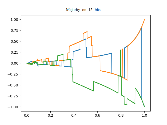
We denote this process by , and by slight abuse of notation, write and . Since is right-continuous, these processes are right-continuous also; when referring to the left limit at jump discontinuities, we write , and , with . Some example sample paths of for the -bit majority function are given in Figure 2.
Since is a piecewise-smooth jump process, by (18) its quadratic variation is equal to the sum of squares of its jumps. Now, almost surely, can make a jump only in one coordinate at a time, and when the -th coordinate jumps, the value of changes by , since is multi-linear. The quadratic variation of is therefore
| (21) |
A crucial property of is that the expected value of these jumps behaves smoothly, as the next lemma shows:
Lemma 13.
Let , and let be a bounded process which satisfies one of the following:
-
1.
is left-continuous and measurable with respect to the filtration generated by .
-
2.
There exists a continuous function such that .
Then
| (22) |
The proof is essentially a change in the order of summation, and involves going over all points in and calculating the jump rate at each point. It is postponed to the appendix.
Corollary 14.
Let . Then for all ,
| (23) |
Proof.
Corollary 15.
Let . Then
Proof.
By the martingale property of ,
Taking the derivative of equation (23) and using the fundamental theorem of calculus on the right hand side gives the desired result. ∎
It is a basic fact (see e.g [GS15, section 4.3]) that if has Fourier expansion , its noise stability is given by
On the other hand, recalling , a short calculation reveals that
Thus and the inequality (10) in the statement of Theorem 8 becomes
Together with equation (23), this turns into
| (24) |
We will use this formulation rather than the original statement of (10).
For every index , let be the harmonic extension of , and let . If is monotone then , since the derivatives are positive, but in general,
| (25) |
by convexity. In particular, plugging (25) into Corollary 14, we have
| (26) |
We call the process the “influence process”, because of how the expectation of its square relates to the influence of : Observe that by (14),
| (27) |
Thus, at time , we have , while at time , since for , we have . The expected value increases from to as goes from to . We denote this expected value by . Equation (26) then becomes
The integral may be more easily handled using a time-change which makes log-convex; we can then bound it by a power of the influence. For this purpose, for , denote .
Lemma 16.
Let be the harmonic extension of a Boolean function, and let . Then is a log-convex function of .
Proof.
Expanding as a Fourier polynomial, we have
| (28) |
This is a positive linear combination of log convex-functions , and is therefore also log-convex [BV04, section 3.5.2]. ∎
Finally, we’ll need the following easy technical lemma, whose short proof is postponed to the appendix.
Lemma 17.
Let be a differentiable function satisfying
| (29) |
where are some positive constants. Suppose that . Then there exists a time , which depends only on and , such that for all
4 Proof of the improved Talagrand’s conjecture
We prove Theorem 4 assuming that improved Keller-Kindler inequality (24) holds; the proof of (24) is found in Section 6. Without loss of generality, we assume that .
The function used in Theorem 4 will be defined by
Recall Doob’s martingale inequality (see e.g [Dur19, Theorem 4.4.4]), which states that if is a non-negative martingale, then
Using this inequality for the non-negative martingale , we thus have
as required by the theorem.
We now turn to prove the inequality (6) using . To this end, we can relate the product to the stochastic constructions in the previous section. By definition of the discrete derivative, for any , if , and if , so
We thus have , and using this relation we define the stochastic process
noting that
Our goal is therefore to bound from below.
A simple calculation, using the fact that is a submartingale, shows that is an increasing function of . For the rest of this section, we therefore assume that
| (30) |
otherwise there is nothing to prove.
Our proof relies on the existence of a stopping time such that with high probability is large, as is shown by the following proposition. Fix whose value is to be chosen later, and define
Proposition 18.
Assuming the above proposition holds, the improved Talagrand’s conjecture swiftly follows:
Proof of Theorem 4.
By conditioning on the event , we have
∎
The rest of this section is devoted to proving Proposition 18. The main idea is to see how different sample paths contribute to the quadratic variation of . On the one hand, the lion’s share of the quadratic variation is gained from paths where the gradient’s norm is large. On the other hand, the quadratic variation has a relatively high probability to be large, and so must be large with relatively high probability as well. This argument takes care of the gradient’s contribution to ; to deal with the supremum’s contribution, we show that with high enough probability, either makes a large jump (which causes both and the gradient’s norm to be large at the same time) or there is a time where ’s position is bounded away from the endpoints , allowing its gradient to be large later on.
Proof of Proposition 18.
Let . Since is a martingale,
and since ,
| (31) |
By conditioning on we have
It remains only to show that for small enough (but fixed) , is larger than some constant.
Since we assume , the process starts at . There are two different ways for to cross above the value : It could either move across it continuously, or it could jump from some value smaller than to some value larger than . We now divide the analysis into two cases, depending on the probability that makes a very large jump over at time .
Case 1: Small jump
Suppose that , i.e with constant probability, no large jump was made at time . The next two propositions show that with high probability the quadratic variation gained from time onward must be large, and that most of the quadratic variation is gained at times when, just before the process jumps, the gradient is large. To make these notions precise, we will need the following definitions. Let
be the event that the norm of the gradient is large just before time ; let
be the event that is large strictly before time ; let
be the quadratic variation accumulated at times when the supremum is large but the gradient is small; and let
be the gain in quadratic variation from time up to and including time .
Proposition 19.
Let , and assume that (30) holds. There exists a function with such that
| (32) |
Proof.
We first express as an integral, rather than a sum over jumps. Since is independent of coordinate , we have that for , . Thus
The process is measurable with respect to the filtration generated by and is left-continuous. Invoking Lemma 13, we have
| (33) |
where the last equality is because can differ from only at discontinuities.
Let be defined as
where is the universal constant from Theorem 8, and set
Consider the integral
The first integral on the right hand side is equal to if . Otherwise, we necessarily have that , in which case the integral can be bounded using equation (24): Since for all , we have
for some constant . Since , the exponent is bounded below by . Since , we thus have that regardless of the value of ,
| (34) |
The second integral on the right hand side can be bounded using the definitions of and : By definition of we have
Proposition 20.
Let and let be a -measurable stopping time such that
for some . Then
This proposition reflects the intuition that for a martingale to reach a point far from its initial position, it should have a large quadratic variation. The proof, however, requires using the particular details of the way the martingale jumps.
Proof.
Let be a number whose value will be chosen later, and let be the first time that the quadratic variation grows beyond . Since the quadratic variation increases only when jumps, and since the probability of jumping at time is , the event is equal to the event , which in turn implies that :
| (38) |
Hence it suffices to bound the probability that . This can be done by looking at the second moment : On one hand, since with probability at least when , we have
giving
| (39) |
On the other hand, can be bounded by considering the size of the jumps of : Since the -algebra generated by the event is contained in that generated by ,
Conditioned on , the process is a martingale for , and so by (19),
By definition of , , and since all jumps are bounded by ,
| (40) |
Plugging this into (38) and (39), we get
Since , this gives
Solving for , we have
In particular, for , we get
∎
With the above two propositions, we can show that . On one hand, by Proposition 19, the expected increase in the quadratic variation from time to time of paths with small gradient must be small: Denoting to be the event that the gradient was small at all times from to , we have
| (41) | ||||
On the other hand, by invoking Proposition 20 with and , the overall increase in quadratic variation is large with high probability:
We then have
Solving for gives
Since , this last expression is larger than some constant for small enough . But the event means that at some time , the gradient was larger than , while the event implies that , yielding . Thus
as needed.
Case 2: Large jump
Suppose now that meaning that with large probability makes a large jump at time to some value greater than :
| (42) |
The next proposition, parallel to Proposition 19, shows that most of the quadratic variation is gained at times when, just after the process jumped, the gradient was large. For a fixed whose value is to be chosen later, let
be the event that the norm of the gradient is large exactly at time , and let
be the quadratic variation accumulated at times when ’s value is large but the gradient is small.
Proposition 21.
Let , and assume that (30) holds. There exists a function with such that
| (43) |
Proof.
The proof is somewhat similar to that of Proposition 19. Observe that the random variable is a function only of ; there is therefore a continuous “interpolating” function such that
Invoking Lemma 13 with , we have
| (44) |
We now define as in Proposition 19, and split the integral in two:
The first integral on the right hand side is dealt with exactly as in Proposition 19, yielding
| (45) |
For the second integral on the right hand side, we again use the fact that is bounded: By definition of ,
| (46) |
whereas
Plugging the above display into (46), we therefore have
Since in any case for some constant , we thus have
| (47) |
Combining (45) and (47), there exists an absolute constant such that
Plugging this into (44) finishes the proof with . ∎
With this proposition in hand, we can show that . Consider the event that at time , both and . Since is the first time that , and since with probability there is no jump at time , this event contributes at least to ; thus
On the other hand, by Markov’s inequality and Proposition 21, this probability is upper-bounded by
Combining the two displays, we get
Taking small enough so that the right hand side is smaller than , we have
For this , under the event , is large:
and so
as needed.
∎
5 Talagrand’s influence inequality and its stability
The proofs of Theorems 2 and 5 are similar in spirit to that of Theorem 3, and again require bounding the gain in quadratic variation. However, extra care is needed to bound the size the individual influence processes .
We first define several quantities which will be central to our proofs. For a fixed whose value will be chosen later, let
| (48) |
be the event that a coordinate had large derivative at the time it jumped; let
and
and let
and
can be thought of as the quadratic variation of the process , but where big jumps (i.e those larger than ) are excluded. Finally, define
Instead of using Theorem 8 to bound influences, we use the following lemma:
Lemma 22.
There exists a universal constant so that
| (49) |
for all .
This lemma can be derived from the hypercontractivity principle (see e.g [CEL12] and [O’D14, Cor. 9.25]). However, we give a different proof based on the analysis of the stochastic process ; this analysis can be pushed further to obtain the stability results. On an intuitive level and in light of equation (22) the lemma shows that all of the “action” which contributes to the variance of the function happens very close to time .
Proof of Lemma 22.
Let to be chosen later. We start by showing that there exists a constant such that
| (50) |
Recall that ; by applying Corollary 15 to the function , we see that satisfies
| (51) |
The right hand side of equation (51) can be bounded using Lemma 9: Taking and in equation (16) and substituting this in equation (51), we have
For ,
| (52) |
By Lemma 17, there exists a time and a constant such that for all ,
where in the last equality we used equation (27) and the fact that . Since , if then
Setting and taking larger than gives the desired result: Equation (50) follows because by equation (14). Note that only if .
Proposition 23.
Proposition 24.
If and , then
The proofs of Propositions 23 and 24 are of a very similar nature to those of Theorem 8 and Propositions 19 and 20.
Proof of Proposition 23.
Since , it is enough to show that
Denoting , by change of variables we get
| (53) |
Let . Assume first that . The integral in equation (53) then splits up into three parts:
| (54) |
For the first integral on the right hand side, we write
Thus
| (55) |
For the second and third integrals, we use the fact that trivially, for all . By Lemma 22, for we then have . The second integral is therefore bounded by
| (56) |
For the third integral, we use the fact that is a decreasing function in (as can be seen from equation (28)). Since and , we immediately have . Putting these bounds together, when we get that
Now assume that . The integral in equation (53) then splits up into two parts:
Again, since is decreasing as a function of and since , the second integral is smaller than the first, and so by (55),
in this case as well. ∎
Proof of Proposition 24.
Assume without loss of generality that (if not, use instead of ; the variances and the probability are the same for both functions). Let . By conditioning on the event , for any we have
We start by bounding the probability . Let , and observe that . Under the event , the process never visited the interval and yet at some point reached a value larger than , and so necessarily had a jump discontinuity of size at least . But a jump occurring at time due to a discontinuity in is of size , and so , implying that . Thus, , and so . Hence
To bound , note that . By the martingale property of ,
and so
Putting this together with the assumption that gives
| (57) |
Next we bound the probability , by relating the quadratic variation to the variance of .
Let be the stopping time . Since the -algebra generated by the event is contained in that generated by ,
Conditioned on , the process is a martingale for , and so by (19),
| (58) |
For the first term on the right hand side, observe that : Since is the sum of squares of the jumps of up to time , the largest value it can attain is plus the square of the jump which occurred at time , and the size of this jump is bounded by . Thus
| (59) |
where the last inequality is by the assumption on and equation (57).
For the second term on the right hand side, since the event forces all jumps to be of size smaller than , we similarly have
| (60) |
Plugging displays (59) and (60) into (58), we get
| (61) |
On the other hand,
and so together with (61) and plugging in and ,
Now, if then stopped because was larger than or equal to . Since is increasing as a function of , as well, and so
| (62) |
Under the event we have that , and by a union bound we get
∎
5.1 Proof of Theorem 2
5.2 Proof of Theorem 5
Lemma 25.
Let be the constant from Lemma 22, and assume that is small enough so that . Then
Proof.
The main assertion involved in proving Theorem 5 connects between the vertex boundary and the probability that the function makes a large jump.
Proposition 26.
For , let be the event defined in equation (48). Then
| (63) |
The prove this proposition, we will construct a modification of , which can be thought of as a “hesitant” version of . For each coordinate , let be the jump set of a Poisson point process on with intensity , independent from (and in particular, independent from the jump process ). Define to be the process such that for every ,
Loosely speaking, there are several ways of thinking about :
-
1.
The process can be seen as a “hesitant” variation of : It jumps with twice the rate (since its set of discontinuities is the union of two Poisson processes with rate ), but half of those times, it returns to the original sign rather inverting it. We refer to this view as the “standard coupling” of with : The process is a copy of , but with additional independent hesitant jumps.
-
2.
The process is equal to at a discrete set of times which follows the law of a Poisson point process with intensity (this is the union ); between two successive zeros it chooses randomly to be either or , each with probability .
Similarly to the notation using , we write , and analogously , and .
Lemma 27.
The process is a martingale.
Proof.
Let . For , since always, we trivially have , so assume .
If , then . Being independent Poisson point processes, almost surely we have , and . Since almost surely, we thus have
It is evident by the definition of the process that
so that .
Proof of Proposition 26.
In order to distinguish between the vertex boundaries, we will use the hesitant jump process defined above. We prove (63) for the inner vertex boundary ; the proof for is identical. Let . Note that for any , we almost surely have that only finitely many times for . Thus, if , then the infimum in the definition of is attained as a minimum, and there exists an such that and . In fact, this holds true if as well: In this case, there is a sequence of times and indices such that and . Since there are only finitely many indices, there is a subsequence so that are all the same index , and the claim follows by continuity of and the fact that .
When occurs, we necessarily have , since whenever is discontinuous. Since is uniform on the hypercube,
and so it suffices to show that
| (64) |
Supposing that , denote by a coordinate for which and . If then ; otherwise, almost surely is the only coordinate of which is , and so for all almost surely. Since the function does not depend on the -th coordinate, we deduce that almost surely. Thus, under , by the martingale property of , we have
| (65) |
Similarly, using the martingale property of , we have , and so
Since is independent of , we finally obtain
∎
Proof of Theorem 5.
Let be the constant from the statement of Lemma 22. Let be such that . Then the condition is satisfied in Lemma 25, implying that . Together with Proposition 26, we have
| (66) |
All that remains is to obtain a lower bound on . To this end, observe that for all , and so . Thus , so there exists a constant such that
Plugging this into (66) gives the desired result. ∎
6 Proof of Theorem 8
As explained above in equation (24), our goal is to show that
| (67) |
We first show that we may assume that is monotone. For an index , define an operator by
The following lemma relates between the influences and sensitivities of and :
Lemma 28 ([BKS99, Lemma 2.7]).
is monotone, and for every pair of indices , and .
Thus, if equation (67) holds for , then it holds for as well, since and . So it’s enough to verify (67) for monotone functions.
In order to prove (67), we may also assume that for any fixed universal constant ,
| (68) |
For if for some , then since is monotone,
and so . Equation (67) then holds trivially with and , since for all .
Similarly, we may assume that for any fixed, universal constant ,
| (69) |
otherwise Theorem 8 would be equivalent (up to constants) to the original theorem proved in [KK13].
Remark 29.
Our proof actually recovers the original theorem proved in [KK13], but we make this assumption since it simplifies some bounds.
Define . At time , we have
The function is monotone in : Since is a martingale, is a submartingale and so is increasing.
By invoking Corollary 15 on , for every index we have
Thus
| (70) |
where is the Hilbert-Schmidt norm of a matrix. By Lemma 10, there exists a continuous positive function such that
Since is continuous it is bounded in , so there exists a constant such that for all ,
| (71) |
By (68), we can assume that . Using (71) together with Lemma 17, there exist constants and a time , all of which depend only on , such that for all ,
In particular, there exists a constant such that
| (72) |
and since is increasing, we can always assume that . Denote ; by Lemma 16, is log-convex in .
Lemma 30.
Let and let be a log-convex decreasing function. Denote and assume that . Then for all ,
Proof.
Consider the function
where is the largest solution to the equation . By choice of , we have
Since is log-linear on , is log-convex on , they have the same integral on and , we must have one of two cases:
-
1.
-
2.
The functions intersect at most once in the interval at some point such that for all .
In either case, for all , we have
| (73) |
On the other hand, we chose to be such that , and so
where the last inequality is by assumption on . The function is decreasing as a function of in the interval , but is greater than 1 at ; hence, since is the largest number for which , we must have . We then have
and after rearranging, since ,
Thus
Putting this into the right hand side of (73) gives
∎
Proof of Theorem 8.
By Corollary 14,
and by change of variables this becomes
Define , where is the constant from equation (72). Note that since and is decreasing,
| (74) |
Rearranging, this gives
| (75) |
Set , and assume without loss of generality that , so that (if , we can take ). This implies that
Invoking Lemma 9 with and , there exists a constant such that
| (76) |
By (69), we can assume that is small enough so (76) implies
| (77) |
Plugging this into (75), we get
For small enough , we have , and so
| (78) |
By Lemma 30 and equations (74) and (75), we have
| (79) |
This allows us to prove (67):
for some universal constant . ∎
References
- [BDC12] Vincent Beffara and Hugo Duminil-Copin, The self-dual point of the two-dimensional random-cluster model is critical for , Probab. Theory Related Fields 153 (2012), no. 3-4, 511–542. MR 2948685
- [BKS99] Itai Benjamini, Gil Kalai, and Oded Schramm, Noise sensitivity of Boolean functions and applications to percolation, Inst. Hautes Études Sci. Publ. Math. (1999), no. 90, 5–43 (2001). MR 1813223
- [BKS03] , First passage percolation has sublinear distance variance, Ann. Probab. 31 (2003), no. 4, 1970–1978. MR 2016607
- [BM00] F. Barthe and B. Maurey, Some remarks on isoperimetry of Gaussian type, Ann. Inst. H. Poincaré Probab. Statist. 36 (2000), no. 4, 419–434. MR 1785389
- [Bob97] S. G. Bobkov, An isoperimetric inequality on the discrete cube, and an elementary proof of the isoperimetric inequality in Gauss space, Ann. Probab. 25 (1997), no. 1, 206–214. MR 1428506
- [BV04] Stephen Boyd and Lieven Vandenberghe, Convex optimization, Cambridge University Press, Cambridge, 2004. MR 2061575
- [CEL12] Dario Cordero-Erausquin and Michel Ledoux, Hypercontractive measures, talagrand’s inequality, and influences, pp. 169–189, Springer Berlin Heidelberg, Berlin, Heidelberg, 2012.
- [CHL97] Mireille Capitaine, Elton P. Hsu, and Michel Ledoux, Martingale representation and a simple proof of logarithmic Sobolev inequalities on path spaces, Electron. Comm. Probab. 2 (1997), 71–81. MR 1484557
- [DS05] Irit Dinur and Samuel Safra, On the hardness of approximating minimum vertex cover, Ann. of Math. (2) 162 (2005), no. 1, 439–485. MR 2178966
- [Dur19] Rick Durrett, Probability—theory and examples, Cambridge Series in Statistical and Probabilistic Mathematics, vol. 49, Cambridge University Press, Cambridge, 2019, Fifth edition of [ MR1068527]. MR 3930614
- [Eld15] Ronen Eldan, A two-sided estimate for the gaussian noise stability deficit, Inventiones mathematicae 201 (2015), no. 2, 561–624.
- [Ell11] David Ellis, Almost isoperimetric subsets of the discrete cube, Combin. Probab. Comput. 20 (2011), no. 3, 363–380. MR 2784633
- [Fri98] Ehud Friedgut, Boolean functions with low average sensitivity depend on few coordinates, Combinatorica 18 (1998), no. 1, 27–35. MR 1645642
- [Fri99] , Sharp thresholds of graph properties, and the -sat problem, J. Amer. Math. Soc. 12 (1999), no. 4, 1017–1054, With an appendix by Jean Bourgain. MR 1678031
- [GKK+09] Dmitry Gavinsky, Julia Kempe, Iordanis Kerenidis, Ran Raz, and Ronald de Wolf, Exponential separation for one-way quantum communication complexity, with applications to cryptography, SIAM J. Comput. 38 (2008/09), no. 5, 1695–1708. MR 2476272
- [GS15] Christophe Garban and Jeffrey E. Steif, Noise sensitivity of Boolean functions and percolation, Institute of Mathematical Statistics Textbooks, vol. 5, Cambridge University Press, New York, 2015. MR 3468568
- [Har76] Sergiu Hart, A note on the edges of the -cube, Discrete Math. 14 (1976), no. 2, 157–163. MR 0396293
- [Kin93] J. F. C. Kingman, Poisson processes, Oxford Studies in Probability, vol. 3, The Clarendon Press, Oxford University Press, New York, 1993, Oxford Science Publications. MR 1207584
- [KK07] Jeff Kahn and Gil Kalai, Thresholds and expectation thresholds, Combin. Probab. Comput. 16 (2007), no. 3, 495–502. MR 2312440
- [KK13] Nathan Keller and Guy Kindler, Quantitative relation between noise sensitivity and influences, Combinatorica 33 (2013), no. 1, 45–71. MR 3070086
- [KKL88] Jeff Kahn, Gil Kalai, and Nathan Linial, The influence of variables on boolean functions (extended abstract), 1988, pp. 68–80.
- [KLS+15] Saleet Klein, Amit Levi, Muli Safra, Clara Shikhelman, and Yinon Spinka, On the converse of talagrand’s influence inequality, CoRR abs/1506.06325 (2015).
- [KR09] Robert Krauthgamer and Yuval Rabani, Improved lower bounds for embeddings into , SIAM J. Comput. 38 (2009), no. 6, 2487–2498. MR 2506299
- [KS06] Gil Kalai and Shmuel Safra, Threshold phenomena and influence: perspectives from mathematics, computer science, and economics, Computational complexity and statistical physics, St. Fe Inst. Stud. Sci. Complex., Oxford Univ. Press, New York, 2006, pp. 25–60. MR 2208732
- [MNT14] Elchanan Mossel, Joe Neeman, and Omer Tamuz, Majority dynamics and aggregation of information in social networks, Autonomous Agents and Multi-Agent Systems 28 (2014), no. 3, 408–429.
- [O’D14] Ryan O’Donnell, Analysis of Boolean functions, Cambridge University Press, New York, 2014. MR 3443800
- [OS07] Ryan O’Donnell and Rocco A. Servedio, Learning monotone decision trees in polynomial time, SIAM J. Comput. 37 (2007), no. 3, 827–844. MR 2341918
- [Raz95] Ran Raz, Fourier analysis for probabilistic communication complexity, Comput. Complexity 5 (1995), no. 3-4, 205–221. MR 1394528
- [Tal93] Michel Talagrand, Isoperimetry, logarithmic Sobolev inequalities on the discrete cube, and Margulis’ graph connectivity theorem, Geom. Funct. Anal. 3 (1993), no. 3, 295–314. MR 1215783
- [Tal94] , On russo’s approximate zero-one law, Ann. Probab. 22 (1994), no. 3, 1576–1587.
- [Tal96] , How much are increasing sets positively correlated?, Combinatorica 16 (1996), no. 2, 243–258. MR 1401897
- [Tal97] , On boundaries and influences, Combinatorica 17 (1997), no. 2, 275–285. MR 1479302
- [Ver18] Roman Vershynin, High-dimensional probability, Cambridge Series in Statistical and Probabilistic Mathematics, vol. 47, Cambridge University Press, Cambridge, 2018, An introduction with applications in data science, With a foreword by Sara van de Geer. MR 3837109
Appendix A Appendix 1: -biased analysis
For , let be the measure
which sets the -th bit to with probability . Let
| (80) |
and for a set , define . Then every function can be written as
| (81) | ||||
| (82) |
The coefficients are called the “-biased” Fourier coefficients of .
The -biased influence of the -th bit is
If is monotone, then
| (83) |
The -biased Fourier coefficients are related to the derivatives of by the following proposition, whose proof (using slightly different notation) can be found in [O’D14, Section 8].
Proposition 31.
Let be a set of indices, , and . Then
Appendix B Appendix 2: Postponed proofs
Proof of Lemma 9.
The lemma is similar to [Tal96, Proposition 2.2], but applied to a biased product distribution rather than to the uniform distribution on . For completeness, we present here a general proof, which does not explicitly use hypercontractivity.
Using (13), the harmonic extension may be written as
where . Since differentiation and harmonic extensions commute, we have
where is the harmonic measure , and . Under this notation,
Let be numbers such that , and let be defined as
Let have distribution . Recall that the sub-gaussian norm of a random variable is defined as , while the sub-gaussian norm of a random vector is defined as (see e.g [Ver18, Sections 2.5 and 3.4] for more about sub-gaussian norms). The random variable is bounded in magnitude by , and so has sub-gaussian norm bounded by for some constant . By [Ver18, Lemma 3.4.2], a random vector with independent, mean-zero sub-gaussian entries is also sub-gaussian, with . Thus the random vector has sub-gaussian norm bounded by as well, which means that for every
Let . Then
Taking gives
for some . In particular,
| (84) |
as well. Now choose , and observe that
Together with (84), this gives the desired result. ∎
Proof of Lemma 10.
Using Proposition 31 for and the fact that ,
| (85) |
The following lemma, which bounds the sum of squares of -biased Fourier coefficients, is immediately obtained from [KK13, Lemma 6].
Lemma 32.
Let and let be such that for all . For a function , let
There exists a function such that for every ,
| (86) |
Proof of Lemma 13.
Assume first that satisfies condition (1), meaning that it is left-continuous and measurable with respect to the filtration generated by . To prove (22), assume first that , so that the number of jumps that makes in the time interval is almost surely finite. For any integer , partition the interval into equal parts, setting for . Since almost surely none of the jumps of occur at any , and since is left-continuous, we almost surely have
Since is bounded, the expression
is bounded in absolute value by a constant times the number of jumps of in the interval , which is integrable. By the dominated convergence theorem, we then have
Since is measurable with respect to , it is independent of whether or not a jump occurred in the interval , and the expectation breaks up into
| (88) |
The set is a Poisson process with rate , and so the number of jumps in the interval distributes as , where
The probability of having at least one jump is then equal to
Plugging this into display (88), we get
The factor is negligible in the limit , since the sum contains only bounded terms. We are left with
Since is continuous almost everywhere, by the definition of the Riemann integral, the limit is equal to , and we get
for all . Taking the limit gives the desired result for by continuity of the right hand side in .
The proof for condition (2), where is similar: Since is right-continuous, we now approximate the sum in the left hand side of (22) using the right-endpoint of the interval:
Using the same reasoning as above we may interchange the expectation and limit, obtaining.
Since is independent of whether or not a jump occurred in the interval , the expectation again breaks up into
From here onwards the proof is identical. ∎
Proof of Lemma 17.
Let , and denote . Note that depends only on . Then for all , we have
Integrating, this means that for all
In particular, , otherwise we’d have , contradicting the definition of and continuity of . Denoting , we must have for all . This ensures that is positive in this interval, which means we can rearrange the differential inequality (29) to give
for all . A short calculation reveals that the left hand side is the derivative of . Integrating from to , we get
Rearranging gives
and exponentiating twice gives the desired result. ∎