How does object fatness impact the complexity of packing in $d$ dimensions?

Abstract

Packing is a classical problem where one is given a set of subsets of Euclidean space called objects, and the goal is to find a maximum size subset of objects that are pairwise non-intersecting. The problem is also known as the Independent Set problem on the intersection graph defined by the objects. Although the problem is NP-complete, there are several subexponential algorithms in the literature. One of the key assumptions of such algorithms has been that the objects are fat, with a few exceptions in two dimensions; for example, the packing problem of a set of polygons in the plane surprisingly admits a subexponential algorithm. In this paper we give tight running time bounds for packing similarly-sized non-fat objects in higher dimensions.

We propose an alternative and very weak measure of fatness called the stabbing number, and show that the packing problem in Euclidean space of constant dimension $d\geqslant 3$ for a family of similarly sized objects with stabbing number $\alpha$ can be solved in $2^{O(n^{1-1/d}\alpha)}$ time. We prove that even in the case of axis-parallel boxes of fixed shape, there is no $2^{o(n^{1-1/d}\alpha)}$ algorithm under ETH. This result smoothly bridges the whole range of having constant-fat objects on one extreme ($\alpha=1$) and a subexponential algorithm of the usual running time, and having very “skinny” objects on the other extreme ($\alpha=n^{1/d}$), where we cannot hope to improve upon the brute force running time of $2^{O(n)}$, and thereby characterizes the impact of fatness on the complexity of packing in case of similarly sized objects. We also study the same problem when parameterized by the solution size $k$, and give a $n^{O(k^{1-1/d}\alpha)}$ algorithm, with an almost matching lower bound: there is no algorithm with running time of the form $f(k)n^{o(k^{1-1/d}\alpha/\log k)}$ under ETH. One of our main tools in these reductions is a new wiring theorem that may be of independent interest.

1 Introduction

Many well-known NP-hard problems (e.g. Independent Set, Hamilton Cycle, Dominating Set) can be solved in time $2^{O(\sqrt{n})}$ when restricted to planar graphs, while only $2^{O(n)}$ algorithms are known for general graphs [23, 28, 16, 30, 13, 12, 14, 15, 18, 11]. This beneficial effect of planarity is known as the “square root phenomenon,” and can be exploited also in the context of 2-dimensional geometric problems where the problem is defined on various intersection graphs in $\mathbb{R}^{2}$ [3, 4, 17, 25]. In particular, consider the geometric packing problem where, given a set of polygons in $\mathbb{R}^{2}$, the task is to find a subset of $k$ pairwise disjoint polygons. This problem can be solved in time $n^{O(\sqrt{k})}$ [25], which – when expressed only a as a function of the input – gives an $n^{O(\sqrt{n})}=2^{O(\sqrt{n}\log n)}$ algorithm for finding a maximum size disjoint subset.

Can these 2-dimensional subexponential algorithms be generalized to higher dimensions? It seems that the natural generalization is to aim for $2^{O(n^{1-1/d})}$ , or in case of parameterized problems, either $2^{O(k^{1-1/d})}\cdot n^{O(1)}$ or $n^{O(k^{1-1/d})}$ time algorithms in $d$-dimensions: the literature contains upper and lower bounds of this form (although sometimes with extra logarithmic factors in the exponent) [9, 26, 29]. However, all of these algorithms have various restrictions on the object family on which the intersection graph is based: there is no known analogue of the $n^{O(\sqrt{k})}$ time algorithm of Marx and Pilipczuk [25] in higher dimensions with the same generality of objects. There is a good reason for this: it is easy to see that any $n$-vertex graph can be expressed as the intersection graph of 3-dimensional simple polyhedra. Thus a subexponential algorithm for 3-dimensional objects without any severe restriction would give a subexponential algorithm for Independent Set on general graphs, violating standard complexity-theoretic assumptions.

What could be reasonable restrictions on the objects that allow running times of the form, e.g., $2^{O(n^{1-1/d})}$? One of the most common restrictions is to study a set $F\subset 2^{\mathbb{R}^{d}}$ of fat objects, where for each object $o\in F$ the ratio $\operatorname{radius}(B_{\mathrm{in}}(o))/\operatorname{radius}(B_{\mathrm{out}}(o))$ is at least some fixed positive constant. (We denote by $\operatorname{radius}(B_{\mathrm{in}})$ and $\operatorname{radius}(B_{\mathrm{out}})$ the radius of the inscribed and circumscribed ball respectively.) Another common restriction is to have similarly sized objects, that is, a family $F$ where the ratio of the largest and smallest object diameter is at most some absolute constant. Many results concern only unit disk graphs, where $F$ consists of unit disks in the plane: unit disks are both fat and similarly sized. The focus of our paper is to explore the role of fatness in the context of packing problems and to understand when and to what extent fatness decreases the complexity of the problem. We observe that fatness is a crucial requirement for subexponential algorithms in higher dimensions, and this prompts us to explore in a quantitave way how fatness influences the running time. For this purpose, we introduce a parameter $\alpha$ describing the fatness of the objects and give upper and lower bounds taking into account this parameter as well.

More precisely, we introduce the notion of the stabbing number, which can be regarded as an alternative measure of fatness. This slightly extends a similar definition by Chan [6]. We say that an object $o$ is stabbed by a point $p$ if $p\in o$. A family of objects $F\subseteq 2^{\mathbb{R}^{d}}$ is $\alpha$-stabbed if for any $r\in\mathbb{R}$, the subset of $F$-objects $o$ of diameter $\operatorname{diam}(o)\in[r/2,r)$ contained in any ball of radius $r$ can be stabbed by $\alpha^{d}$ points. The stabbing number of $F$ is defined as $\inf_{\alpha\in[1,\infty)}\{F\text{ is $\alpha$-stabbed}\}$. Note that a set of $n$ objects in $d$-dimensions has stabbing number at most $n^{1/d}$. The stabbing number is closely related to the inverse of a common measure of fatness. This relationship is explored in Section 2.

By adapting a separator theorem from [9], we can give an algorithm where the running time smoothly goes from $2^{O(n^{1-1/d})}$ to $2^{O(n)}$ as the stabbing number goes from $O(1)$ to the maximum possible $n^{1/d}$.

Theorem 1.1.

Let $\alpha\in[1,\infty)$ and $2\leqslant d\in\mathbb{N}$ be fixed constants. There is an algorithm that solves Independent Set for intersection graphs of similarly sized $\alpha$-stabbed objects in $\mathbb{R}^{d}$ running in time $2^{O(n^{1-1/d}\alpha)}$.

As mentioned, the stabbing number is at most $n^{1/d}$, and this algorithm runs in subexponential time whenever the stabbing number is better than this trivial upper bound, that is, whenever $\alpha=o(n^{1/d})$ holds.

In order to have definite answers to the best running times achievable, we also need a lower bound framework. A popular starting point in the past decades is the Exponential Time Hypothesis (ETH) [21], which posits that there exists a constant $\gamma>0$ such that there is no $2^{\gamma n}$ algorithm for the $3$-SAT problem. Classical NP-hardness reductions automatically yield quantitative lower bounds on the running time under ETH. If enough care is taken to ensure that the constructed instance is sufficiently small, then one can find lower bounds that match the best known algorithms [8]. For the Independent Set problem, a lower bound of $2^{\Omega(n)}$ is a consequence of classical reductions under ETH.

A standard way to explore the impact of a parameter such as fatness is to give an algorithm where the parameter appears in the running time, together with a matching lower bound. However, the notion of “matching lower bound” needs to be defined precisely if we are expressing the running time as a function of two parameters, the size $n$ of the instance and the stabbing number $\alpha$ of the objects.

A recent example of such an algorithm and lower bound involving two parameters is the paper by Biró et al. [5], where it is shown that the coloring problem of unit disk graphs with $\ell=n^{\lambda}$ colors can be solved in $2^{O(\sqrt{n\ell}\log n)}$ time, where $\lambda\in[0,1]$ is a fixed constant, and they also exclude algorithms of running time $2^{o(\sqrt{n\ell})}$ under ETH. This is interesting since this smoothly bridges the gap between a standard “square root phenomenon” algorithm ($\ell=O(1))$) on one extreme and the brute force $2^{O(n)}$ on the other ($\ell=n^{1-o(1)}$). Our results show a similar behavior in the context of fatness and the packing problem: the running time of Theorem 1.1 is optimal, with the running time smoothly going from $2^{O(n^{1-1/d})}$ time in the case of $\alpha=O(1)$ to the trivial $2^{O(n)}$ timeof brute force when $\alpha=n^{1/d}$.

Let $\mathcal{G}(d,L)$ denote the set of intersection graphs in $\mathbb{R}^{d}$ where each object is an axis-parallel box whose side lengths form the multiset $\{1,\dots,1,L\}$. Let us call such an axis-parallel box canonical. As usual, $n$ denotes the number of objects (the number of vertices in the graph).

For example, it is easy to see that $1\times 1\times L$ boxes have stabbing number $O(L^{2/3})$. Any collection of $1\times 1\times L$ boxes of the same orientation can be stabbed by the lattice generated by the vertices of such a box, which has $O(L^{2})$ points in a ball of radius $O(L)$. By taking the same lattice for the two other orientations, we obtain a complete stabbing set of size $O(L^{2})$ inside a ball of radius $O(L)$ for all axis-parallel boxes of this shape. In general for $d\geqslant 3$, the stabbing number for canonical boxes is $\alpha=O(L^{1-1/d})$, so in particular, for $L=1$ we have $\alpha=O(1)$, and for $L\geqslant n^{1/(d-1)}$ we have $\alpha=O(n^{1/d})$. In our main contribution, we show that this very restricted set of non-fat objects is sufficient to prove the desired lower bound.

Theorem 1.2.

Let $d\geqslant 3$ be fixed. Then there is a constant $\gamma>0$ such that for all $\alpha\in[1,n^{1/d}]$ it holds that Independent Set on intersection graphs of $d$-dimensional canonical axis-parallel boxes of stabbing number $\alpha$ has no algorithm running in time $2^{\gamma n^{1-1/d}\alpha}$, unless ETH fails.

An immediate corollary is that the $2^{O(n)}$ time brute-force algorithm cannot be improved, even for the intersection graph of axis-parallel boxes. This Corollary 1.3 can also be derived from a simpler construction by Chlebík and Chlebíková [7].

Corollary 1.3.

Let $3\leqslant d\in\mathbb{N}$ be fixed. Then Independent Set on intersection graphs of axis-parallel boxes in $d$-dimensions has no algorithm running in time $2^{o(n)}$, unless ETH fails.

In unit ball graphs, there is a lower bound of $2^{\Omega(n^{1-1/d})}$ under ETH, which of course carries over to intersection graphs of fat objects [9]. This latter reduction is based on establishing efficient routing constructions (called the “Cube Wiring theorem”) in the $d$-dimensional Euclidean grid. The crucial insight of the present paper is that tight lower bounds for nonfat objects can be obtained via Independent Set on induced subgraphs of the $d$-dimensional blown-up grid cube, where each vertex is replaced by a clique of $t$ vertices, fully connected to the adjacent cliques in all $d$ directions. First we establish a lower bound for Independent Set on subgraphs of such cubes (even for subgraphs of maximum degree 3), using and extending the Cube Wiring theorem [9]. Unlike for unit balls, it now seems difficult to realize every such subgraph $G$ as intersection graph of appropriate boxes. Instead, we realize a graph $G^{\prime}$ that is obtained from $G$ by some number of double subdivisions (subdividing some edge twice). As every double subdivision is known to increase the size of the maximum independent set by exactly 1, switching to $G^{\prime}$ does not cause a problem in the reduction.

The key insight of the reduction (in 3-dimensions) is that if $t=L^{2}$, then $t$ vertices can be represented with $1\times 1\times L$ size boxes arranged in an $L\times L$ grid, occupying $O(L)\times O(L)\times O(L)$ space. Each $t$-clique of the blown-up cube is represented by such arrangements of boxes. The main challenge that we have to overcome is that the subgraph $G$ may contain an arbitrary matching between two adjacent $t$-cliques. Given two sets of $1\times 1\times L$ size boxes arranged in two $L\times L$ grids, it seems unclear whether such arbitrary connections can be realized while staying in an $O(L)\times O(L)\times O(L)$ region of space. However, we show that this is possible, as the $L\times L$ grid arrangement allows easy reordering within the rows or within the columns, and it is known that any permutation of a grid can be obtained as doing a permutation first within the rows, then within the columns, and finally one more time within the rows. Thus with some effort, it is possible to build gadgets representing $L\times L$ vertices in an $O(L)\times O(L)\times O(L)$ region of space that allows arbitrary matchings to be realized with the adjacent gadgets.

The idea is similar in higher dimensions $d>3$. We reduce from the Independent Set problem on a subgraph of the blow-up of a $d$-dimensional grid where each vertex is blown-up into a clique of $L^{d-1}$ vertices. Each gadget now contains $L^{d-1}$ boxes of size $1\times 1\times\dots\times 1\times L$ arranged in a grid. In order to implement arbitrary matchings between adjacent gadgets, we decompose every permutation of the $(d-1)$-dimensional grid into $O(d)$ simpler permutations that are easy to realize in $d$-dimensional space.

We also study the complexity of packing in the context of parameterized algorithms: the question is how much one can improve the brute force $n^{O(k)}$ algorithm for finding $k$ independent objects. We present a counterpart of Theorem 1.1 in this setting.

Theorem 1.4.

Let $\alpha\in[1,\infty)$ and $2\leqslant d\in\mathbb{N}$. There is a parameterized algorithm that solves independent set for intersection graphs of similarly sized $\alpha$-stabbed objects in $\mathbb{R}^{d}$ running in time $n^{O(k^{1-1/d}\alpha)}$, where the parameter $k$ is the size of the maximum independent set.

If one regards the parameterized algorithm’s running time in terms of the instance size only, the result would be a $2^{O(n^{1-1/d}(\log n)\alpha)}$ algorithm, which is slower than the running time $2^{O(n^{1-1/d}\alpha)}$ provided by the latter algorithm. The parameterized algorithm is based on a separator theorem by Miller et al. [27].

Finally, we sketch how the lower bound construction of Theorem 1.2 can be adapted to a parameterized setting, and obtain the following theorem:

Theorem 1.5.

Let $3\leqslant d\in\mathbb{N}$ be fixed. Then there is a constant $\gamma>0$ such that for all $\alpha\in[1,n^{1/d}]$ it holds that deciding if there is an independent set of size $k$ in intersection graphs of $d$-dimensional canonical axis-parallel boxes of stabbing number $\alpha$ has no $f(k)n^{\gamma k^{1-1/d}\alpha/\log k}$ algorithm for any computable function $f$, unless ETH fails.

The crucial difference is that we are reducing from the Partitioned Subgraph Isomorphism problem instead of Independent Set, which means that instead of choosing or not choosing a box (representing choosing or not choosing a vertex in the Independent Set problem), the solution needs to choose one of $n$ very similar boxes (representing the choice of one of $n$ vertices in a class of the partition). The overall structure of the reduction (e.g., routing in the blown-up $d$-dimensional grid) is similar to the proof of Theorem 1.2.

Organization. In Section 2 we establish some bounds that relate the stabbing number to fatness. Section 3 presents both our non-parameterized and parameterized algorithm. In Section 4 we prove the wiring theorem that is necessary for both of our lower bounds. Sections 5 and 6 contain our lower bounds for the non-parameterized and parameterized problem respectively. Finally, Section 7 draws some conclusions and proposes two open problems.

2 The relationship between the stabbing number and fatness

In the usual definition of fatness, an object $o\subset\mathbb{R}^{d}$ is $\alpha$-fat if there exists a ball of radius $\rho_{\mathrm{in}}$ contained in $o$ and a ball of radius $\rho_{\mathrm{out}}$ that contains $o$, where $\rho_{\mathrm{in}}/\rho_{\mathrm{out}}=\alpha$. For a fixed constant $\alpha$ this is a useful definition and unifies many other similar notions in case of convex objects, i.e., it holds that a set of convex objects that is constant-fat for this notion of fatness are constant-fat for more restrictive definitions and vice versa. For our purposes however this definition is not fine-grained enough in the following sense. The fatness of a $1\times 1\times n$ box in three dimensions would be $\Theta(n)$, just as the fatness of a $1\times n\times n$ box. As it will be apparent in what follows, we need a fatness definition according to which $1\times n\times n$ boxes are much more fat than $1\times 1\times n$ boxes. For this purpose, we use the following weaker definition of fatness, that tracks the volume compared to a circumscribed ball more closely. (Note that constant-fat objects are also weakly constant-fat.)

Definition 2.1 (Weakly $\alpha$-fat).

A measurable object $o\subseteq\mathbb{R}^{d}$ is $\alpha$-fat for some $\alpha\in[1,\infty)$ if $Vol(o)/Vol(B)\leqslant\alpha^{d}$, where $Vol(o)$ and $Vol(B)$ denotes the volume of $o$ and the volume of its circumscribed ball $B$ respectively.

An object $o$ is strongly $\alpha$-fat if for any ball $B$ centered inside $o$ we have $Vol(B\cap o)/Vol(B)\geqslant\alpha^{d}$. In case of convex objects, weak fatness coincides with strong fatness up to constant factors, see [31].

The next theorem shows that the inverse of the weak fatness of an object family is related to the stabbing number. In a sense, this means that the stabbing number is a further weakening of weak fatness. Note that in our setting, the stabbing number will be polynomial in $n$ (i.e., $\alpha=n^{\lambda}$ for some constant $\lambda$), so the $\log n$ term is insignificant.

Theorem 2.2.

Let $d$ be a fixed constant. Then the stabbing number of any family of $n$ weakly $(1/\alpha)$-fat (measurable) objects in $\mathbb{R}^{d}$ is $O(\alpha\log^{1/d}n)$.

Proof 2.3.

Consider a family $F$ of weakly $1/\alpha$-fat objects. Let $B$ be a ball of radius $\delta$, and let $F_{B}$ be the set of objects contained in $B$ of diameter at least $\delta/2$. It is sufficient to show that we can stab $F_{B}$ with $O(\alpha^{d}\log n)$ points. Pick $k=\left\lfloor(4\alpha)^{d}(\log n+1)\right\rfloor$ points $p_{1},\dots p_{k}$ independently uniformly at random in $B$. For any given object $o$, its volume is at least $\operatorname{Vol}(B)/(4\alpha)^{d}$, so the probability that a given $p_{i}$ is not in $o$ is at most $1-1/(4\alpha)^{d}$. Since the $k$ points are chosen independently, the probability that a given object $o$ is unstabbed is at most $\left(1-\frac{1}{(4\alpha)^{d}}\right)^{k}$. By the union bound, the probability that there is an unstabbed object is at most

$$n\left(1-\frac{1}{(4\alpha)^{d}}\right)^{k}=n\left(1-\frac{1}{(4\alpha)^{d}}\right)^{\left\lfloor(4\alpha)^{d}(\log n+1)\right\rfloor}<n(1/e)^{\log n+1}<1.$$

Consequently, there exists an outcome where all objects are stabbed.

We conclude this section with the following theorem, which shows an even stronger connection between fatness and stabbing in case of convex objects. The theorem uses the existence of the John ellipsoid [22] and the $\varepsilon$-net theorem [20].

Theorem 2.4.

Let $d$ be a fixed constant. Then the stabbing number of any family of $n$ weakly $(1/\alpha)$-fat convex objects in $\mathbb{R}^{d}$ is $O(\alpha\log^{1/d}\alpha)$.

Proof 2.5.

Consider a family $F$ of weakly $1/\alpha$-fat convex objects. Let $B$ be a ball of radius $\delta$, and let $F_{B}$ be the set of objects contained in $B$ of diameter at least $\delta/2$. It is sufficient to show that we can stab $F_{B}$ with $O(\alpha^{d}\log\alpha)$ points. For any given object $o$, its volume is at least $\operatorname{Vol}(B)/(4\alpha)^{d}$. Every convex object $o\in F_{B}$ contains an ellipsoid $\ell(o)\subseteq o$ such that $\operatorname{Vol}(o)/\operatorname{Vol}(\ell(o))\leqslant d^{d}$ [22]. Since the VC-dimension of ellipsoids in $\mathbb{R}^{d}$ is $O(d^{2})$ [2], the $\epsilon$-net theorem [20] implies that the ellipsoids $\ell(o)\;(o\in F_{B})$ can be stabbed by $O(\frac{d^{2}}{1/(4\alpha)^{d}}\log\frac{d^{2}}{1/(4\alpha)^{d}})=O(\alpha^{d}\log\alpha)$ points. Since the ellipsoids are contained in their respective objects, this point set also stabs all objects in $F_{B}$.

3 Algorithms

We require very little from the objects that we use in our algorithms. It is necessary that we can decide in polynomial time whether a point is contained in an object, whether two objects intersect, and whether an object intersects some given sphere, ball, and empty or dense hypercube. Let us assume that such operations are possible from now on.

3.1 An algorithm with weighted cliques

The algorithm for Theorem 1.1 is an adaptation of the Independent Set algorithm for fat objects from [9], based on weighted cliques.

Proof 3.1 (Proof of Theorem 1.1).

The algorithm works by finding a balanced separator of the objects, such that the separator itself can be partitioned into cliques and this partition has the property that the number of independent sets within the separator is $2^{O(n^{1-1/d}\alpha)}$. The result then follows from applying this algorithm recursively. Thus, we are left with the task to prove the existence of such a separator.

We begin by picking a minimum size hypercube $H_{0}$ that contains at least $n/(6^{d}+1)$ objects, and we translate and scale everything so that $H_{0}$ becomes a unit hypercube centered at the origin. We now define $n^{1/d}$ hypercubes $H_{1},\ldots,H_{n^{1/d}}$, which will be our candidate separators. Each hypercube $H_{i}$ is centered at the origin and has edge length $1+\frac{2i}{n^{1/d}}$.

Each hypercube $H_{i}$ corresponds to a separator as follows: the separator consists of the objects intersected by the boundary of the hypercube, and separates the objects contained in the interior of the hypercube from those that do not intersect it. To ensure that the separators are balanced, to each separator we add all objects intersecting $H_{n^{1/d}}$ with diameter $\geqslant 1/4$. Note that these objects can be stabbed with $O(1)$ points, and therefore do not contribute too many cliques to the partition.

Lemma 3.2.

Each separator $H_{i}$ is balanced, in the sense that both the interior and exterior contain at most $\frac{6^{d}}{6^{d}+1}n$ objects.

Proof 3.3.

Due to the choice of $H_{0}$ the interior of each separator contains at least $n/(6^{d}+1)$ objects. Thus, the exterior of each separator contains at most the claimed number of objects.

To see that the interior does not contain too many objects either, consider the separator associated with $H_{n^{1/d}}$. Since all objects with radius $\geqslant 1/4$ are contained in the separator, we only need to show that $H_{n^{1/d}}$ contains at most $(n6^{d})/(6^{d}+1)$ objects with radius $<1/4$. Note that $H_{n^{1/d}}$ has side length $3$, and thus volume $3^{d}$. Consider a subdivision of $H_{n^{1/d}}$ into $6^{d}$ sub-hypercubes of side length $1/2$. The objects (of radius at most $1/4$) intersecting any such given sub-hypercube are contained in a hypercube of edge length strictly less than one. Note that $H_{0}$ is the smallest hypercube containing at least $n/(6^{d}+1)$ objects. Therefore, at most $n/(6^{d}+1)$ objects intersect each sub-hypercube, and thus $H_{n^{1/d}}$ contains at most $(n6^{d})/(6^{d}+1)$ objects of radius $<1/4$.

Next, we show that among the separators $H_{1},\ldots,H_{n^{1/d}}$, at least one has a suitable partition into cliques. Consider a separator $S$ and a partition of $S$ into cliques $\mathcal{C}(S)=C_{1},\ldots,C_{k}$. Then the weight of $S$ is $\Sigma_{C\in\mathcal{C}(S)}\gamma(|C|)$, where $\gamma$ is a weight function and $|C|$ denotes the number of vertices of the clique $C$. We set $\gamma(n)=\log(n+1)$, but the result holds for any function $\gamma(n)=O(n^{1-1/d})$.

Given a partition of $S$ into cliques, the number of independent sets in $S$ is at most

$$\prod_{C\in\mathcal{C}(S)}(|C|+1)=2^{\sum_{C\in\mathcal{C}(S)}\log(|C|+1)}.$$

We show that the total weight of all separators is $O(n\alpha)$; since there are $n^{1-1/d}$ candidate separators, it follows that there exists a separator with weight $O(n^{1-1/d}\alpha)$. Such a separator therefore has $2^{O(n^{1-1/d}\alpha)}$ independent sets.

In the following, let $\beta$ denote the volume of the circumscribed ball of the smallest object, and note that since the objects are similarly sized, all circumscribed balls have the same volume up to a constant factor. Note that, because $H_{0}$ contains $n/6^{d}$ objects and we performed a scaling such that $H_{0}$ has size $1$, we have $\beta<1$. We distinguish two cases: if $\beta^{1/d}>{n^{-1/d}}$ or $\beta^{1/d}\leqslant{n^{-1/d}}$.

Case 1:

$\beta^{1/d}>{n^{-1/d}}$.

Since $\beta<1$, all balls intersecting the separator are contained in a hypercube $O(1+\beta)=O(1)$, which can be covered by $O(1/\beta)$ balls of volume $\beta$. By the definition of the stabbing number, it is possible to stab all the objects intersecting the separators using $O(\frac{1}{\beta}\alpha^{d})$ points, and thus there is a partition of the objects into $O(\frac{1}{\beta}\alpha^{d})$ cliques, which we denote by $C_{1},\dots,C_{k}$.

The total weight of the cliques $C_{1},\dots,C_{k}$ is

$$\sum_{i=1}^{k}\gamma(|C_{i}|)=O(\sum_{i=1}^{k}(|C_{i}|)^{1-1/d}).$$

The right hand side here is maximized if the number of cliques is maximum (i.e., we have $c\frac{1}{\beta}\alpha^{d}$ cliques for some constant $c$) and each clique contains the same number of objects (i.e., $\frac{n}{c\frac{1}{\beta}\alpha^{d}}$ objects). Furthermore, since the diameter of the union of objects in any clique is $O(\beta^{1/d})$ and the distance between consecutive separators is $1/n^{1/d}$, each clique contributes weight to at most $O(\beta^{1/d}n^{1/d})$ separators. Therefore, the total weight (of all separators) is at most

$$O\left(\beta^{1/d}n^{1/d}\cdot\frac{1}{\beta}\alpha^{d}\cdot\gamma\left(\frac{n}{\frac{1}{\beta}\alpha^{d}}\right)\right)=O(n\alpha),$$

since $\gamma(t)=O(1^{1-1/d})$. There are $n^{1/d}$ separators, thus at least one of them must have weight at most $O(n^{1-1/d}\alpha)$.

Case 2:

$\beta^{1/d}\leqslant{n^{-1/d}}$.
Each clique contributes to the weight of at most $O(1)$ separators. The total weight of all separators is then at most a constant times the total weight of the cliques. This can be upper bounded by $O(\sum_{i=1}^{k}|C_{i}|^{1-1/d})$, which by the concavity of $x^{1-1/d}$ is $O(n)$. Thus, there is a separator with weight at most $O(n^{1-1/d})$.

3.2 A parameterized algorithm with a sphere separator

To prove Theorem 1.4, we use the following separator theorem, due to Miller et al. [27]. The ply of a set of objects in $\mathbb{R}^{d}$ is the largest number $p$ such that there exists a point $x\in\mathbb{R}^{d}$ which is contained in $p$ objects.

Theorem 3.4 (Miller et al. [27]).

Let $\Gamma=\{B_{1},\ldots,B_{n}\}$ be a collection of $n$ closed balls in $\mathbb{R}^{d}$ with ply at most $p$. Then there exists a sphere $S$ whose boundary intersects at most $O(p^{1/d}n^{1-1/d})$ balls, and the number of balls in $\Gamma$ disjoint from $S$ that fall inside and outside $S$ are both at most $\frac{d+1}{d+2}n$.

We can now prove Theorem 1.4.

Proof 3.5 (Proof of Theorem 1.4).

Let $F$ be the set of similarly-sized objects with stabbing number $\alpha$ defining the intersection graph. Consider the set of balls $B$ made up by the circumscribed balls of the objects of $F$ that are in a maximum independent set. We claim that the ply of this set is $O(\alpha^{d})$. To prove the claim, let $S$ be a subset of the independent set whose circumscribed balls overlap at a point $x\in\mathbb{R}^{d}$. Since the objects are similarly sized, $S$ must lie within a ball centered at $x$ whose radius is at most a constant times the diameter of the largest object. Thus, $S$ can be stabbed by $O(\alpha^{d})$ points. However, as $S$ forms an independent set, each point can only stab at most one object from $S$. Therefore, $|S|=O(\alpha^{d})$.

By Theorem 3.4 the ball set $B$ has a $\frac{d+1}{d+2}$-balanced sphere separator, where the sphere intersects $O((\alpha^{d})^{1/d}k^{1-1/d})$ $=O(k^{1-1/d}\alpha)$ balls. We proceed by guessing such a sphere, but in order to do that, we need to define a polynomially large set of spheres to guess from.

All that is important about a sphere $\sigma$ is the separation that it performs on $B$, that is, it splits $B$ to the set of balls inside, the set of balls outside, and the set of balls intersected by $\sigma$. Given an arbitrary sphere $\sigma$, we shrink it while we can without making it disjoint from any of the originally intersected balls, or until a new ball is touched that was inside the sphere originally. As a result, we get a canonical sphere $\sigma^{\prime}$ that is tangent to some set of balls from $B$. Note that such spheres can be uniquely defined by a set of at most $d+1$ tangent balls, and a string that for each of these balls describes if they are inside or outside $\sigma^{\prime}$. In order to define $\sigma$, we add another bit for each touching ball, which is set if and only if the ball was originally not intersected by $\sigma$. Therefore, the number of guesses we can make for $\sigma$ is $n^{d+1}4^{d+1}$. Notice that the guess defines the sets of balls inside, outside and intersected by $\sigma$ as well.

After guessing $\sigma$, we proceed by guessing which of the objects intersected by $\sigma$ are in the solution, and remove the remaining objects intersected by $\sigma$. Since at most $O(k^{1-1/d}\alpha)$ of the intersected objects are in the solution, there are $n^{O(k^{1-1/d}\alpha)}$ possibilities for this guess.

From the remaining objects, we remove those that are adjacent to the objects guessed to be in the solution, and recurse on the objects inside $\sigma$ and on the objects outside $\sigma$ separately. The running time $T(n,k)$ for this algorithm satisfies the recurrence (for fixed $d$):

$$T(n,k)=n^{O(k^{1-1/d}\alpha)}\cdot T\left(n,k\cdot\frac{d+1}{d+2}\right)$$

which implies the running time $T(n,k)=n^{O(k^{1-1/d}\alpha)}$.

For arbitrary size objects that are $O(1)$-fat in some stronger sense (or just $O(1)$-stabbed), we can apply the above scheme of guessing a separating sphere or hypercube, and use one of the many separator theorems designed for objects of small ply. See [29, 6, 19]. One can also apply [9] since in case of ply $1$, the weights are constants; although the theorem is stated for the usual notion of fatness, the proof itself uses only the stabbing number. We get the following theorem.

Theorem 3.6.

Let $2\leqslant d\in\mathbb{N}$. There is a parameterized algorithm that solves Independent Set for intersection graphs of $O(1)$-stabbed objects in $\mathbb{R}^{d}$ running in time $n^{O(k^{1-1/d})}$, where the parameter $k$ is the size of the maximum independent set.

4 Wiring in a blowup of the Euclidean Cube

Our wiring theorem relies on the folklore observation that can be informally stated the following way: an $n\times m$ matrix can be sorted by first permuting the elements within each row, then permuting the elements within each column, and then permuting the elements in each row again. Note that the permutations are independent of each other, and they are not sorting steps; the permutations required are quite specialized. We state the lemma in a more group-theoretic setting. Let $Sym(X)$ denote the symmetric group on the set $X$.

Lemma 4.1 (Lemma 4 of [1]).

Let $A$ and $B$ be two finite sets. Then $Sym(A\times B)=G_{A}G_{B}G_{A}$, where $G_{A}$ is the subgroup of $Sym(A\times B)$ consisting of permutations $\pi$ where $\pi(a,b)\in A\times\{b\}$ for all $(a,b)\in A\times B$, and $G_{B}$ is the subgroup of $Sym(A\times B)$ consisting of permutations $\pi$ where $\pi(a,b)\in\{a\}\times B$ for all $(a,b)\in A\times B$.

Corollary 4.2.

Let $2\leq d\in\mathbb{N}$ and let $A_{1},A_{2},\dots,A_{d}$ be finite sets. Then $\Gamma\mathrel{\overset{\makebox[0.0pt]{\mbox{\tiny def}}}{=}}Sym(A_{1}\times A_{2}\times\dots\times A_{d})$ is of the form $\Gamma=G_{1}G_{2}\dots G_{d-1}G_{d}G_{d-1}G_{d-2}\dots G_{1}$, where $G_{i}$ is the subgroup of $\Gamma$ consisting of permutations $\pi$ where $\pi(a_{1},\dots,a_{i},\dots,a_{d})\in\{a_{1}\}\times\dots\times\{a_{i-1}\}\times A_{i}\times\{a_{i+1}\}\times\dots\times\{a_{d}\}$ for all $(a_{1},\dots,a_{d})\in\Gamma$.

Proof 4.3.

We use induction on $d$; for $d=2$, the statement is equivalent to Lemma 4.1. Let $d\geq 3$. We can write $\Gamma$ as $Sym\big{(}(A_{1}\times\dots\times A_{d-1})\times A_{d}\big{)}$, so by induction (for $d=2$), we have that $\Gamma=G_{1}\times G_{A_{2}\times\dots\times A_{d}}\times G_{1}$. By induction, we also have that $G_{A_{2}\times\dots\times A_{d}}=G_{2}\dots G_{d-1}G_{d}G_{d-1}G_{d-2}\dots G_{2}$, therefore $\Gamma=G_{1}G_{2}\dots G_{d-1}G_{d}G_{d-1}G_{d-2}\dots G_{1}$.

For an integer $n$, let $[n]=\{1,\dots,n\}$. Let $\mathcal{EC}^{d}(n)$ be the $d$-dimensional Euclidean grid graph whose vertices are $[n]^{d}$, and $x,y\in V(G)$ are connected if and only if they are at distance $1$ in $\mathbb{R}^{d}$. For $x\in\mathbb{Z}^{d}$ and $S\subset\mathbb{Z}^{d}$, we use the shorthand $x+S\mathrel{\overset{\makebox[0.0pt]{\mbox{\tiny def}}}{=}}\{x+y\;|\;y\in S\}$. Let $\mathcal{BEC}^{d}(n,t)$ denote the $t$-fold blowup of $\mathcal{EC}^{d}(n)$, where all vertices of $\mathcal{EC}^{d}(n)$ are exchanged with a clique of size $t$, and vertices in neighboring cliques are connected. More precisely,

$$V(\mathcal{BEC}^{d}(n,t)) =[n]^{d}\times[t]$$

$$E(\mathcal{BEC}^{d}(n,t)) =\big{\{}(x,i)(y,j)\;\big{|}\;x=y\vee(x,y)\in E(\mathcal{EC}^{d}(n))\big{\}}.$$

Our second key ingredient is the Euclidean Cube Wiring theorem.

Theorem 4.4 (Theorem 21 in [9]).

Let $3\leq d\in\mathbb{Z}$. There exists a constant $c$ dependent only on the dimension such that any matching $M$ between $P=[n]^{d-1}\times\{1\}$ and $Q\mathrel{\overset{\makebox[0.0pt]{\mbox{\tiny def}}}{=}}[n]^{d-1}\times\{cn\}$ can be embedded in $\mathcal{EC}^{d}(cn)$, that is, there is a set of vertex disjoint paths connecting $p$ and $q$ in $\mathcal{EC}^{d}(cn)$ for all $pq\in M$.

Theorem 4.5 (Blown-up Cube Wiring).

Let $3\leq d\in\mathbb{Z}$, and let $n,t$ be positive integers. We consider two opposing facets of the blown-up cube $\mathcal{C}\mathrel{\overset{\makebox[0.0pt]{\mbox{\tiny def}}}{=}}\mathcal{BEC}^{d}(cn,t)$ (where $c\in\mathbb{Z}_{+}$ depends only on $d$):

$$P \mathrel{\overset{\makebox[0.0pt]{\mbox{\tiny def}}}{=}}\big{(}[n]^{d-1}\times\{1\}\big{)}\times[t]$$

$$Q \mathrel{\overset{\makebox[0.0pt]{\mbox{\tiny def}}}{=}}\big{(}[n]^{d-1}\times\{cn\}\big{)}\times[t]$$

Any matching $M$ between $P$ and $Q$ can be embedded in $\mathcal{C}$, that is, there is a constant integer $c$ dependent only on the dimension $d$ such that for any matching $M$ there is a set of vertex disjoint paths connecting $p$ and $q$ in $\mathcal{BEC}^{d}(cn,t)$ for all $pq\in M$.

Proof 4.6.

Without loss of generality, suppose that $M$ is a perfect matching between $P$ and $Q$ (this can be ensured by adding dummy edges to $M$ if necessary). Let $c=c^{\prime}+2$ where $c^{\prime}$ is a constant such that cube wiring can be done in height $h=c^{\prime}n$. Let $A=[n]^{d-1}$ and let $B=[t]$. The matching $M$ can be regarded as a permutation $\pi$ of $A\times B$, where $\pi(a,b)=(a^{\prime},b^{\prime})$ if $\big{(}(a,b)(a^{\prime},b^{\prime})\big{)}\in M$.

By Lemma 4.1, there exists a permutation $\pi_{A}\in G_{A}$ and $\pi_{B},\pi^{\prime}_{B}\in G_{B}$ such that $\pi=\pi^{\prime}_{B}\pi_{A}\pi_{B}$, where $G_{A}$ and $G_{B}$ are defined as in Lemma 4.1. We can think of both $\pi_{B}$ and $\pi^{\prime}_{B}$ as the union of $n^{d-1}$ distinct permutations of $[t]$. We can realize $\pi_{B}$ using one matching: for all $(x,i)\in A\times B$, we add the edge $((x,1),i)((x,2),j)$ to $M_{B}$, where $\pi_{B}(x,i)=(x,j)$. As a result, $M_{B}$ is a perfect matching between $P$ and the next layer of the blown-up cube, $P^{\prime}\mathrel{\overset{\makebox[0.0pt]{\mbox{\tiny def}}}{=}}\big{(}[n]^{d-1}\times\{2\}\big{)}\times[t]$. Similarly, for all $(x,i)\in A\times B$, let $M^{\prime}_{B}$ contain the edge $((x,cn-1),i)((x,cn),j)$, where $\pi^{\prime}_{B}(x,i)=(x,j)$; this matches $Q^{\prime}\mathrel{\overset{\makebox[0.0pt]{\mbox{\tiny def}}}{=}}\big{(}[n]^{d-1}\times\{cn-1\}\big{)}\times[t]$ to $Q$. Finally, by the Cube Wiring Theorem (Theorem 4.4), for each $i\in[t]$, there are vertex disjoint paths from $P^{\prime}_{i}\mathrel{\overset{\makebox[0.0pt]{\mbox{\tiny def}}}{=}}\big{(}[n]^{d-1}\times\{2\}\big{)}\times\{i\}$ to $Q^{\prime}_{i}\mathrel{\overset{\makebox[0.0pt]{\mbox{\tiny def}}}{=}}\big{(}[n]^{d-1}\times\{cn-1\}\big{)}\times\{i\}$ that realizes the matching

$$M^{i}_{A}\mathrel{\overset{\makebox[0.0pt]{\mbox{\tiny def}}}{=}}\{(x,i)(y,i)\mid x\in[n]^{d-1}\text{ and }\pi_{A}(x,i)=(y,i)\}.$$

For each $i\in[t]$, these wirings are vertex disjoint since they are contained in vertex disjoint Euclidean grid hypercubes. The matchings $M^{i}_{A}$ for $i\in[t]$ together with the matchings $M_{B}$ and $M^{\prime}_{B}$ realize the matching $M$.

5 Lower bounds for packing isometric axis-parallel boxes

Our first lower bound shows that the running time of the algorithm in Theorem 1.1 is tight under ETH.

Overview of the proof of Theorem 1.2. Our proof is a reduction from $(3,3)$-SAT, the satisfiability problem of CNF formulas where clauses have size at most three and each variable occurs at most three times. Such formulas have the property that if they have $n$ variables, then they have $O(n)$ clauses. The problem has no $2^{o(n)}$ algorithm under ETH [10].

The proof has two steps; the first step is a reduction form $(3,3)$-SAT to Independent Set in certain subgraphs of the blown-up Euclidean cube, and the second step is to show that these subgraphs can essentially be realized with axis-parallel boxes. Throughout the proof, we consider the dimension $d$ to be a constant.

The incidence graph of a $(3,3)$-CNF formula $\phi$ is a graph where vertices correspond to clauses and variables of $\phi$, and a variable and clause vertex are connected if and only if the variable occurs in the clause.

5.1 Independent Set in subgraphs of the blown-up Euclidean cube

A simple and generic lower bound construction for Independent Set.

We give a generic reduction from $(3,3)$-SAT to Independent Set, which serves as a skeleton for the more geometric type of reduction we will do later.

Consider the incidence graph of $\phi$. Replace each variable vertex $v$ with a cycle of length $6$, consisting of vertices $v^{1},\dots,v^{6}$, where the edges formerly incident to $v$ are now connected to distinct cycle vertices $v^{2},v^{4}$ or $v^{6}$ for positive literals and to $v^{1},v^{3}$ or $v^{5}$ for negative literals (see Figure 1). We replace each clause vertex $w$ that corresponds to a clause of exactly $3$ literals with a cycle of length three, and connect the formerly incident edges to distinct vertices of the triangle. For clauses that have exactly two literals, the gadget is a single edge, and we connect the formerly incident edges to distinct endpoints of the edge. We can eliminate clauses of size $1$ in a preprocessing step. Let $G^{\prime}_{\phi}$ be the resulting graph.

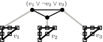
Figure 1: The graph $G_{\phi}$ for $\phi=(v_{1}\vee\neg v_{2}\vee v_{3})$

An independent set can contain at most $3$ vertices of a variable cycle of length $6$, and at most $1$ vertex per clause gadget. Observe that a formula with $\nu$ variables and $\gamma$ clauses has an independent set of size $3\nu+\gamma$ if and only if the original formula is satisfiable.

Let $G$ be a graph and let $uv$ be an edge of $G$. A double subdivision of $uv$ is replacing $uv$ with a path of length $3$, i.e., we add the new vertices $w$ and $w^{\prime}$, remove the edge $uv$ and add the edges $uw,ww^{\prime},w^{\prime}v$. A graph that can be obtained from $G$ by some sequence of double subdivisions is called an even subdivision of $G$. Observe that a double subdivision increases the size of the maximum independent set by one, so $G$ has an independent set of size $k$ if and only if its even subdivision $G^{\prime}$ has an independent set of size $k+\frac{|V(G^{\prime})|-|V(G)|}{2}$.

Embedding $G^{\prime}_{\phi}$ into a blown-up cube.

In a blown-up cube $\mathcal{BEC}^{d}(n,t)$, we call a clique corresponding to $x\in[n]^{d}$ the cell of $x$ or simply a cell, that is, the cell of $x$ is defined as the set of vertices $\{x\}\times[t]\subset V(\mathcal{BEC}^{d}(n,t))$.

The following is a tight lower bound for Independent Set inside the blown-up Euclidean cube.

Theorem 5.1.

For any fixed constant $d\geqslant 3$, there exists a $\gamma>0$ such that for any $t\geqslant 2$ there is no $2^{\gamma n^{1-1/d}t^{1/d}}$ algorithm for Independent Set for subgraphs of the blown-up cube $\mathcal{C}\mathrel{\overset{\makebox[0.0pt]{\mbox{\tiny def}}}{=}}\mathcal{BEC}^{d}((n/t)^{1/d},t)$ under ETH. The lower bound holds even if the subgraph $G$ has maximum degree three, and the neighbors of each vertex in $G$ lie in distinct cells.

Proof 5.2.

Given a $(3,3)$-SAT formula $\phi$, we show that we can construct a subgraph of a blown-up cube with the required properties that is also an even subdivision of $G^{\prime}_{\phi}$. If $\phi$ has $\bar{n}$ literals, then we create a subgraph $G$ that has $n=c\cdot\bar{n}^{\frac{d}{d-1}}/t^{\frac{1}{d-1}}$ vertices for some constant $c$ which will be specified later. Let $s\mathrel{\overset{\makebox[0.0pt]{\mbox{\tiny def}}}{=}}(n/t)^{1/d}$ denote the side length of $\mathcal{C}$. Note that $|V(\mathcal{C})|=s^{d}t=n$.

First, we embed an even subdivision of $G^{\prime}_{\phi}$ into $\mathcal{C}$ as explained next. We use the bottom and the top “layers” of the blown-up cube to embed the variable cycles and clause cycles respectively. Let $P$ and $Q$ be the point sets corresponding to the bottom and top layer of cells respectively, i.e., $P\mathrel{\overset{\makebox[0.0pt]{\mbox{\tiny def}}}{=}}\big{(}[s]^{d-1}\times\{1\}\big{)}\times[t],\qquad Q\mathrel{\overset{\makebox[0.0pt]{\mbox{\tiny def}}}{=}}\big{(}[s]^{d-1}\times\{s\}\big{)}\times[t].$ We embed each variable cycle of $G^{\prime}_{\phi}$ into $P$: we (injectively) associate six vertices of even intra-cell index in six cells of $P$, that is, a variable cycle on vertices $v_{1}\dots v_{6}$ is associated with the vertices $(x^{(1)},2k),\dots,(x^{(6)},2k)$ in this order, where $x^{(1)},\dots x^{(6)}$ is a cycle in the bottom facet of $\mathcal{EC}^{d}(s)$ and $k\in[t/2]$. As we will see below, if $|P|$ is large enough, then we can pick $x^{(1)},\dots x^{(6)}$ and $k$ for each variable cycle so that this association is injective.

With each clause, we associate a pair or triplet of vertices in $Q$ that are in neighboring cells, more precisely, for clauses of size three, the vertices are of the form $(x,k),(x,k+1),(x^{\prime},k)$, while for clauses of size two we have $(x,k),(x^{\prime},k)$ for some $(x,x^{\prime})\in E(\mathcal{EC}^{d}(s))$ and $k\in[t-1]$. If $|Q|$ is large enough, then we can pick $x$ and $k$ for each clause so that the association remains injective.

Let $\mathsf{Var}$ be the set of vertices in $\mathcal{C}$ corresponding to vertices on the variable cycles with a wire connection. Let $\mathsf{Cla}$ be the set of vertices in $\mathcal{C}$ assigned to the clauses. Note that the number of literals is $|\mathsf{Cla}|=|\mathsf{Var}|=\bar{n}$, and we have that

$$\begin{split}|P|=|Q|=s^{d-1}t=(n/t)^{\frac{d-1}{d}}t=\left(\frac{c\cdot\bar{n}^{\frac{d}{d-1}}/t^{\frac{1}{d-1}}}{t}\right)^{\frac{d-1}{d}}\cdot t=c^{\frac{d-1}{d}}\bar{n}.\end{split}$$

By picking $c\geqslant 6$, we ensure that there is enough space to do the above associations injectively for any $d\geqslant 3$, as we will have $|P|=|Q|>3\bar{n}$.

Let $M$ be the perfect matching between $\mathsf{Var}$ and $\mathsf{Cla}$ given by $\phi$. By Theorem 4.5, there is a wiring from $\mathsf{Var}$ to $\mathsf{Cla}$ realizing $M$, as long as $c$ is a large enough constant. Crucially, observe that $|P|=|Q|=\Theta(s^{d-1}t)$ means that $P$ and $Q$ occupy a constant fraction of the vertices in the cells of the top and bottom facet of $\mathcal{C}$, so the wiring given by Theorem 4.5 is dense in the sense that a constant fraction of all vertices of $\mathcal{C}$ is induced by the wiring.

Next, in $Q$, we add an edge or triangle for each pair or triplet of vertices assigned to a clause. In $P$, for each vertex $(x,2k)\in\mathsf{Var}$ that is the endpoint of a wire of even length, we add an edge $((x,2k),(x,2k-1))$, and regard $(x,2k-1))$ as the new endpoint of this wire. Finally, for each six-tuple of wire endpoints corresponding to a variable, we add a $6$-cycle.

The graph $G^{\prime}$ created this way clearly has the desired properties: it is a subgraph of $\mathcal{C}$ that has maximum degree three, and the neighbors of each vertex in $G^{\prime}$ lie in distinct cells. Moreover, $G^{\prime}$ can be constructed in $O(n)=\operatorname{poly}(\bar{n})$ time.

By the properties of even subdivisions of $G^{\prime}_{\phi}$, we know that $G^{\prime}$ has an independent set of a certain size if and only if $\phi$ is satisfiable. Suppose that for all $\gamma>0$ there is an $\exp\left(\gamma n^{1-1/d}t^{1/d}\right)$ algorithm for Independent Set. This would result for all $\gamma>0$ in a $(3,3)$-SAT algorithm with running time

$$\exp\left(\gamma c\cdot\bar{n}^{\frac{d}{d-1}}/t^{\frac{1}{d-1}}\right)^{1-1/d}\cdot t^{1/d}+\operatorname{poly}(\bar{n})=2^{(\gamma c)^{1-1/d}\cdot\bar{n}}+\operatorname{poly}(\bar{n}).$$

The existence of such algorithms contradicts ETH.

5.2 Detailed construction and gadgetry

Having established our lower bound for blown-up Euclidean cubes, we now need to construct a set of canonical boxes whose intersection graph is an even subdivision of a given subgraph with maximum degree three where the neighbors of each vertex lie in distinct cells.

Theorem 5.3.

Let $d\geqslant 3$ and $L\geqslant 16$ be fixed, and let $G$ be a subgraph of the blown-up cube $\mathcal{C}=\mathcal{BEC}^{d}(s,(L/8)^{d-1})$ of maximum degree three, where the neighbors of each vertex lie in distinct cells. Then $G$ has an even subdivision $G^{\prime}$ that can be realized using boxes of size $1\times\dots\times 1\times L$. Moreover, given $G$, the boxes of $G^{\prime}$ can be constructed in $O(|V(\mathcal{C})|)$ time, and $|V(G^{\prime})|=O(|V(G)|)$.

We proceed with the proof of Theorem 5.3. We consider $d=3$ first; later on, we show how the construction can be generalized to higher dimensions. We need to define a set of boxes whose intersection graph is an even subdivision of $G$. The idea is to create a generic module that is able to represent a subgraph of $G$ induced by any cell; these modules will take up $O(L)\times O(L)\times O(L)$ space. The modules are arranged into a larger cube of side length $O(sL)$ to make up the final construction.

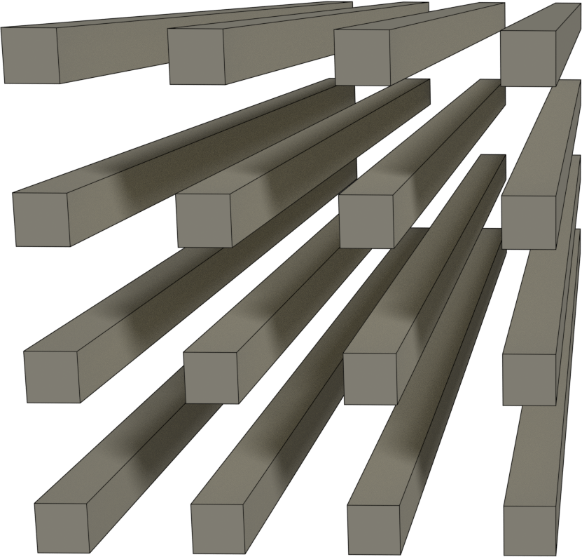
Figure 2: A basic brick.

Modules and bricks.

We index the vertices in a cell by a pair from $[L/8]^{2}$. The starting object in our reduction is a set of $(L/8)^{2}$ disjoint boxes parallel to the same axis, arranged loosely in an $L/8\times L/8$ grid structure called a brick. See Figure 2 for an example. Loosely speaking, each box of each brick within the cell’s module can be associated with a vertex of the cell; for a brick $B$, we can refer to a box corresponding to vertex $(i,j)$ of the cell as $B(i,j)$.

Let $X$ be the set of cells within $\mathcal{C}$: $X\mathrel{\overset{\makebox[0.0pt]{\mbox{\tiny def}}}{=}}\big{\{}\{x\}\times[L/8]^{2}\;\big{|}\;x\in[cn]^{d}\big{\}}$. The wiring within each cell $x\in X$ will be represented by $O(1)$ bricks, and these bricks will fit in an $O(L)$ side length module.

The position of a brick can be specified by defining its axis (along which the side length of the boxes is $L$), and for each box $(i,j)$ within the brick, defining the coordinates of its lexicographically smallest corner (or lexmin corner for short). For example, consider the brick $B$ with axis $x_{3}$ where box $B(i,j)$ has coordinates $(3i,3j,0)$. (See Figure 2.) This brick and all bricks isometric to this are called basic bricks. Most bricks can be thought of as a perturbation of a basic brick, where we apply shifts to each box. The eventual module that we create will consist of several bricks, which together will represent an even subdivision of the sparse graph $G$ restricted to a given cell. Note that no single brick can be said to represent the set of vertices in a cell. When defining our gadgetry, it is convenient to talk about these bricks, even though in the final construction we only need a certain subset of the boxes within each brick. We can remove the unwanted boxes from each brick at a later stage.

Parity Fix, adjustment, bridge, and elbow gadgets.

The parity fix gadget is introduced so that we can ensure that each of the subdivisions that we create are even subdivisions. The gadget induces a path of length $3$ or $4$ depending on our needs, but occupies the same space in both cases. More precisely, the parity fix gadget contains three or four boxes, depending on the parity we need. The union of the boxes is a larger box of size $3L\times 1\times 1$; it is easy to see that within that space we can realize both a path of length three and four using $L\times 1\times 1$ boxes: one can cover the larger box by placing their lexmin corners at equal length intervals.

We can bridge distance along the axis of a basic brick by putting basic bricks next to each other, where each box intersects only the box of the same index from the previous and following brick. This creates a set of $(L/8)^{2}$ vertex disjoint paths in the intersection graph. We call this a bridge gadget.

Using two bricks of the same axis, we can in one step get rid of a perturbation (or introduce one). Let $B$ be a normal brick with axis $x_{3}$ that is a perturbation of the basic brick. We introduce the basic brick $B^{\prime}$ that is the translate of the basic brick with the vector $(0,1,L/2)$. Notice that box $B(i,j)$ intersects $B^{\prime}(i,j)$ and no other boxes. Moreover, we could even introduce arbitrary perturbations along the $x_{1}$ axis in $B^{\prime}$ and along the $x_{3}$ axis within both $B$ and $B^{\prime}$ without changing the intersection graph induced by $B$ and $B^{\prime}$. We call a pair of normal bricks that are a translated and rotated version of these an adjustment gadget.

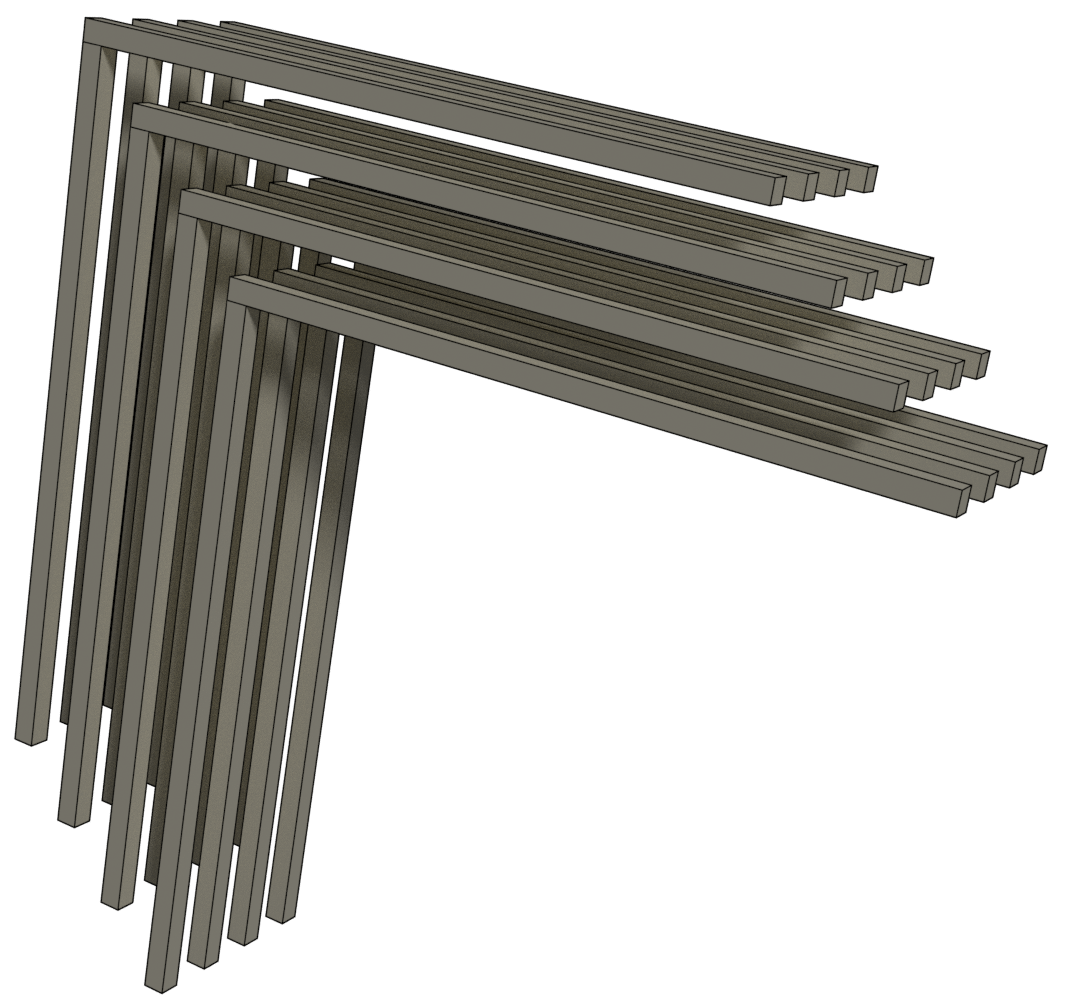
Figure 3: An elbow.

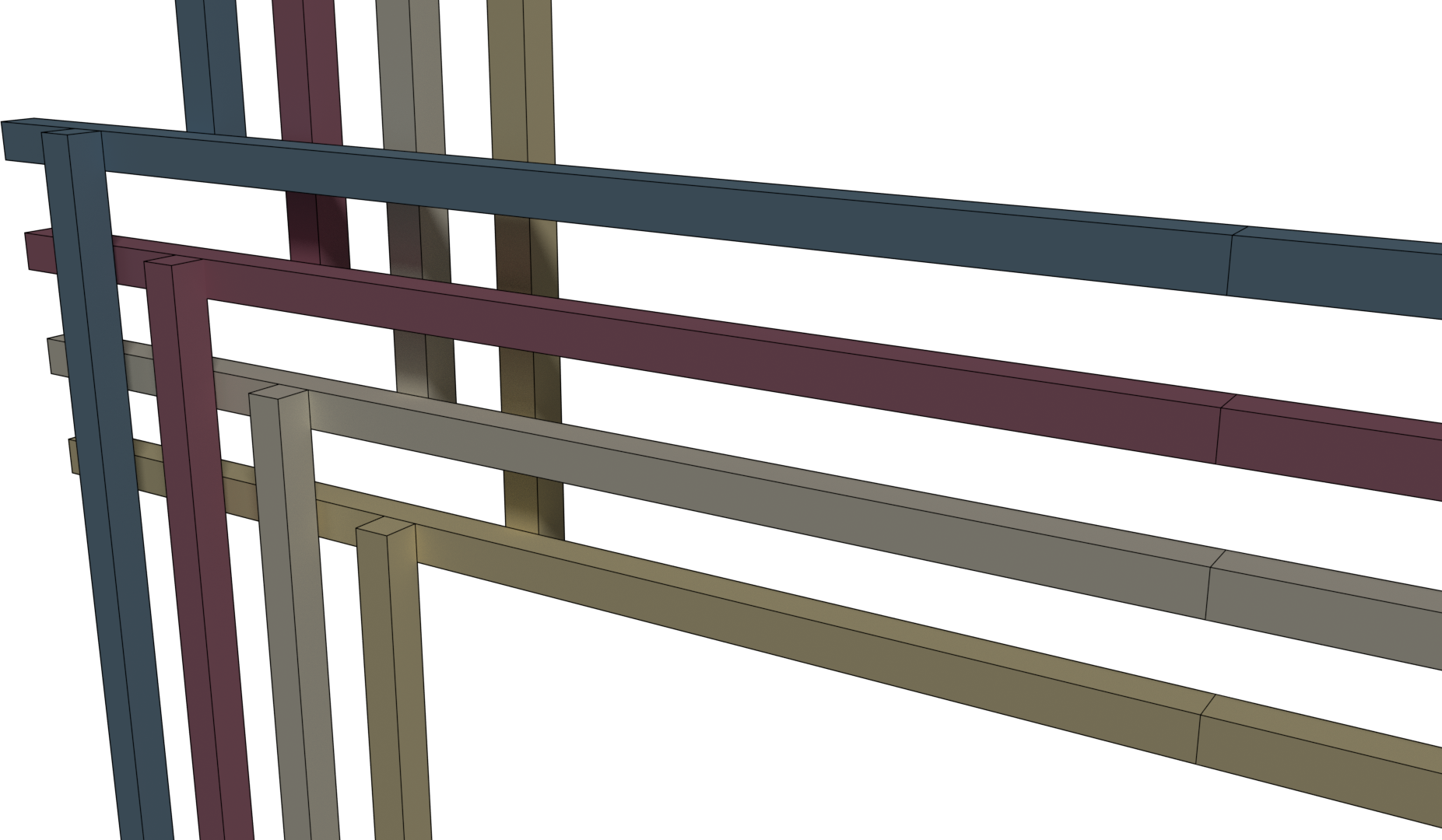
Figure 4: The first “column” of a branching gadget.

Next, we introduce a way to change brick axis using an “elbow”. Consider a brick $B$ that is a perturbation of the basic brick, where box $(i,j)$ has coordinates $(3i,3j,-3i)$. The brick $B^{\prime}$ has axis $x_{1}$ and the coordinates for $B^{\prime}(i,j)$ are $(3i,3j,L-3i)$ (see Figure 3). Notice that using these elbow gadgets and adjustment gadgets together, one can route from any brick to any other brick at distance $\Theta(L)$ in $O(1)$ steps.

The parallel matching gadget.

A parallel matching gadget is capable of realizing a matching between two cells where the endpoints of each matching edge differ only on a fixed coordinate, so for $d=3$, all edges are of the type $\big{(}(x,(i,j)),(x^{\prime},(i^{\prime},j))\big{)}$ or all edges are of the type $\big{(}(x,(i,j)),(x^{\prime},(i,j^{\prime}))\big{)}$ for some cells $x$ and $x^{\prime}$.We call a matching with this property a parallel matching. Parallel matchings can be decomposed into matchings on disjoint cliques, where each clique contains vertices that share all of their coordinates except one. In the remainder of this gadget’s description, we will omit the cells $x$ and $x^{\prime}$ from the coordinate lists.

Suppose that each matching edge is of the form $\big{(}(i,j),(i^{\prime},j)\big{)}$. Let $\pi_{j}(i)$ denote the first coordinate of the pair of $(i,j)$, that is, suppose that the matching edges are $\big{(}(i,j),(\pi_{j}(i),j)\big{)},\;i\in I_{j}$ for some sets $I_{j}\subseteq[L/8]$. Instead of realizing these matchings, we first extend them to permutations $\pi_{j}$ on each clique $[L/8]\times\{j\}$. A permutation can be thought of as a perfect matching between two copies of a set; by removing the unwanted vertices (removing the unwanted boxes) we can get to a representation of the matching, i.e., a set of vertex disjoint paths that connect box $(i,j)$ in the starting brick to box $(\pi_{j}(i),j)$ in the target brick.

In every brick, each box is translated individually, where the translation vector’s component along the brick’s axis must be an integer $k\in 3\cdot\{-L/8,\dots,L/8\}$, and along the other axes it must be of the form $k/L$ for some $k\in\{-L/8,\dots,L/8\}$. For a brick $B$, its box of index $(i,j)$ is denoted by $B(i,j)$, and recall that the position of a box is defined by its lexmin corner and the axis of the brick.

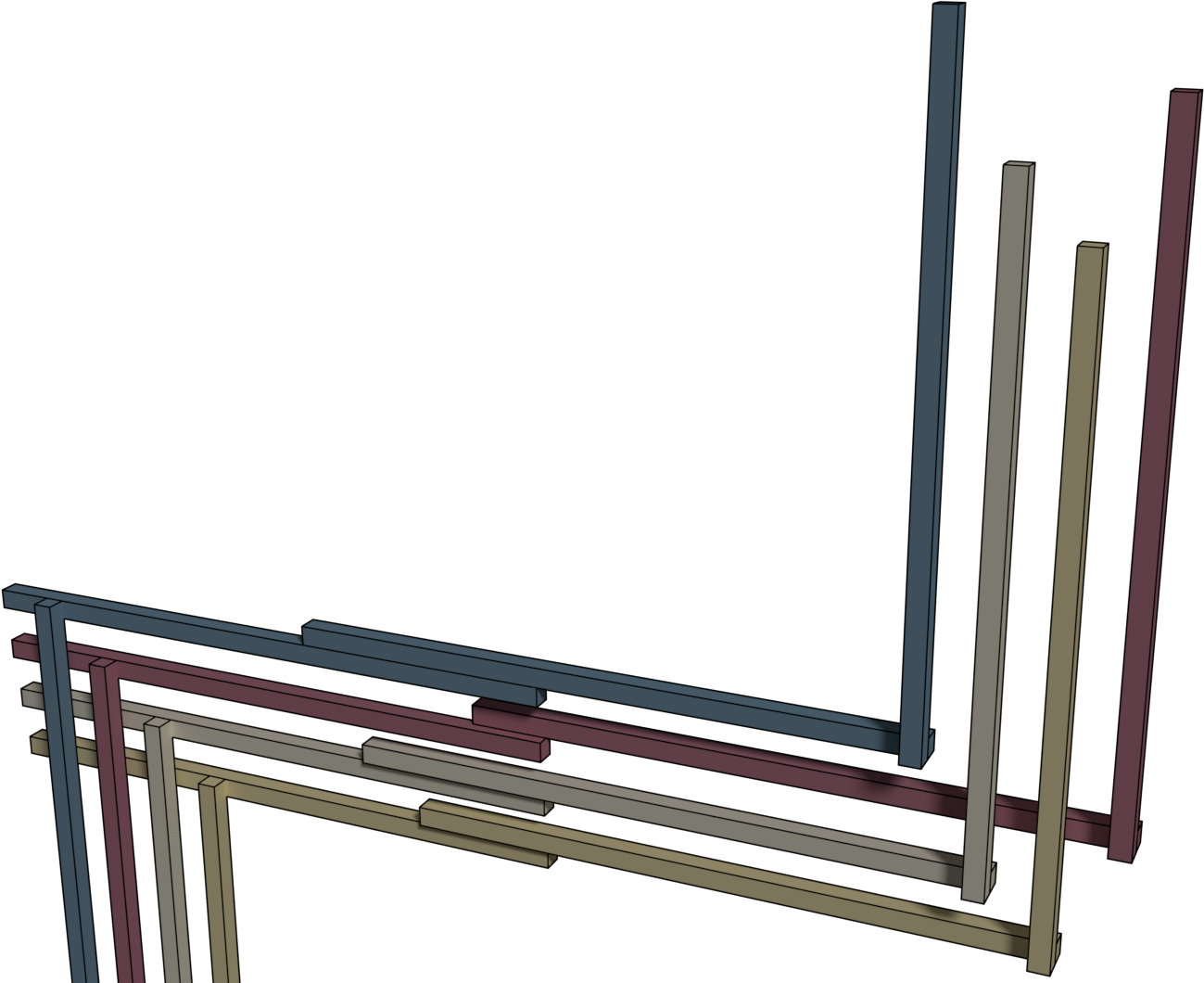
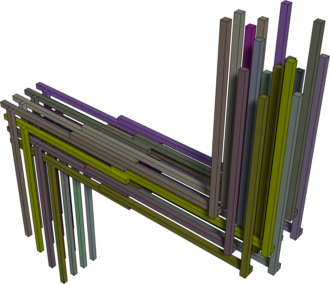
Figure 5: Left: First column of a parallel matching gadget for the permutation $\pi_{1}(1)=1,\pi_{1}(2)=4,\pi_{1}(3)=2,\pi_{1}(4)=3$. Boxes of each color induce paths; boxes of different color are disjoint. Right: A full parallel matching gadget.

We give the coordinates of each box in each brick of the parallel matching gadget below. Let us take the matching edges where $j=1$ first. We start with the first column of the brick ($j=1$), where the coordinates of $B^{(1)}(i,1)$ are $(3i,3+i/L,-3i)$. See the left hand side of Figure 5 that illustrates the idea behind the gadget. The coordinates for $B^{(1)}(i,j)$ are $(3i,3j+i/L,-3i)$. The first column of the next brick $B^{(2)}$ has axis $x_{1}$ and the coordinates of $B^{(2)}(i,1)$ are $(0,4+i/L,L-1-3i)$, that is, these boxes touch the previously defined boxes of $B^{(1)}$ from “behind” in Figure 5. In general, $B^{(2)}(i,j)$ has coordinates $(0,3j+1+i/L,L-3i)$. The next brick $B^{(3)}$ also has axis $x_{1}$, and the coordinates for $B^{(3)}(i,j)$ are $(L/2+3\pi_{j}(i),3j+1+\pi_{j}(i)/L,L-3i)$, that is, we change the box perturbations along the first and second coordinate. Finally, the last brick $B^{(4)}$ has axis $x_{3}$ and the coordinates are $(3L/2+3\pi_{j}(i),3j-\pi_{j}(i)/L,L-3i)$, i.e., they are placed “in front of” the bricks of $B^{(3)}$ in Figure 5. This can be rewritten as $B^{(4)}(i^{\prime},j)$ having coordinates $(3L/2+3i^{\prime},3j-i^{\prime}/L,L-3\pi^{-1}_{j}(i^{\prime}))$. Notice that in the final brick, we indeed have the desired ordering, i.e., the ordering of the boxes along the $x_{1}$ axis is as required. It is routine to check that the intersection graph induced each column of this parallel matching gadget consists of vertex disjoint paths of length four. Different columns are also disjoint since projecting the boxes of column $j$ onto the $x_{2}$ axis results in a subset of the open interval $(3j-0.5,3j+2.5)$.

Realizing an arbitrary matching of a biclique or clique.

We can regard a general matching $M$ induced by two neighboring cells as a permutation of $[L/8]^{2}$, which can be written as the product of three special permutations by Corollary 4.2 that correspond to parallel matchings; i.e., the matching $M$ is realizable as the succession of three parallel matchings. This means that each edge of $M$ becomes a path of length three, so by using three parallel matching gadgets in succession we can represent $M$. We add a parity fix gadget to each box at the beginning of each wire, which will be useful later to ensure that each edge has been subdivided an even number of times. As a result, we have realized $M$ using $O(1)$ bricks and $O(L)\times O(L)\times O(L)$ space. This collection of boxes is called a general matching gadget. A general matching gadget has a first and a last brick where it connects to the rest of the construction, we call these bricks endbricks.

If the goal is to realize a matching within a cell with vertex set $V_{x}$, then we can just create two copies of $V_{x}$ (denoted by $V^{\prime}_{x}$ and $V^{\prime\prime}_{x}$), with a complete bipartite graph between them. For a matching edge $v_{i}v_{j}\in\binom{V_{x}}{2}$, we identify it with the edge $v_{i}^{\prime}v_{j}^{\prime\prime}$. Then we realize the matching of this biclique using a general matching gadget.

The branching gadget.

The branching gadget creates for all indices in $[L/8]^{2}$ a disjoint copy of a star on $4$ vertices (that is, a vertex of degree $3$ with its neighborhood of $3$ isolated vertices). This gadget contains four bricks, and realizes $(L/8)^{2}$ disjoint stars. We use the first two bricks ($B^{(1)}$ and $B^{(2)}$) of the parallel matching gadget. The third brick $B^{\prime}$ is a translate of the first brick $B^{(1)}$ with the vector $(3,2,L-1)$, i.e., the coordinates of $B^{\prime}(i,j)$ are $(3i+3,3j+2+i/L,L-1-3i)$. The final brick $B^{\prime\prime}$ is the translate of $B^{(2)}$ by the vector $(L,0,0)$. See Figure 4 for a rendering of the first “column” of the four bricks. Vertices corresponding to $B^{(2)}$ have degree three, and their neighbors are the boxes of the same index in $B^{(1)}$, $B^{\prime}$ and $B^{\prime\prime}$.

Constructing a module.

Our goal is to define modules of side length $O(L)$ that are capable of representing the role played by cells. The modules together must be able to represent a subgraph of $\mathcal{C}$ of maximum degree three, where the neighbors of any vertex lie in distinct cells.

For all pairs of neighboring modules, we introduce a general matching gadget to represent the matching required by $G$ between the two neighboring cells. These gadgets form the interface. Moreover, in the middle of each module, we add another general matching gadget to represent the matching within the cell; this gadget is the core of the module. See Figure 6. Finally, within each module, we tie the endbricks of the core and the endbricks of the interface falling inside the module together with a brick-tree. The brick-tree is a collection of $(L/8)^{2}$ isomorphic and disjoint trees, realized as a collection of branching, elbow, adjustment and bridge gadgets. Each tree $(i,j)$ has maximum degree three, and its leaves are the boxes of index $(i,j)$ in the interface and in the core.

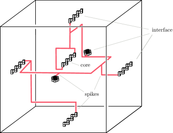
Figure 6: A module with general matching gadgets of the interface and the core, with the simplified image of a brick-tree (in red).

First, we show that such a construction is sufficient to represent an even subdivision of an arbitrary subgraph $G$, and later we show how the brick-tree can be constructed. Let $G$ be a subgraph with the desired properties, and let $x$ be a particular cell. For each edge $uv$ induced by $x$, we fix an arbitrary orientation, and realize the acquired matching so that the source vertex of the arcs are in one end of the core and the targets are in the other. Since the neighbors of any vertex lie in different cells, all indices of $[L/8]^{2}$ appear at most once, either as a source of an arc, as a target of an arc, or not at all. Then we realize the arcs using the core’s general matching gadget of the module. For each index $\mathbf{i}\in[L/8]^{2}$, the edges incident to vertex $\mathbf{i}$ of $x$ can be assigned to a subtree $T$ of the tree corresponding to index $\mathbf{i}$, where $T$ has at most three leaves, at most one of which is adjacent to a box of the core, and other leaves are adjacent to boxes in distinct endbricks of the interface. There is a unique minimal subtree $T$ that induces the desired (at most three) leaves; we can map a vertex $v\in V(G)$ of degree three to the degree three vertex of $T$. If $V$ has a smaller degree, then it can be mapped to an arbitrary non-leaf vertex of $T$.

To construct a brick-tree in $\mathbb{R}^{3}$, consider first a Euclidean grid cube of size $O(1)$. We can use this small cube as a model of our module: in general, an edge of this cube represents a brick. We have some edges already occupied by the general matching gadgets corresponding to the interface and the core. By choosing a cube large enough, we can ensure that these vertices are distant in the $\ell_{1}$ norm. It is easy to see that if the cube is large enough (we allow its size to depend only on $d$), then there is a subtree of the grid of maximum degree three, where the leaves are some distant prescribed vertices. Such a tree can be constructed for example by mimicking a Hamiltonian path of the inscribed octahedron of the module, and adding to it small “spikes” that go to the endbrick of the interfaces. At the end of the path, we extend it towards the center of the cube, where we add another branching for the two endbricks of the core. The branching points in the brick-tree are branching gadgets, the turns are elbow gadgets, and straight segments are bridges and adjustments.

Finalizing the construction in $\mathbb{R}^{3}$.

By packing the modules in a side length $O(sL)$ Euclidean cube, and removing unused boxes from each module according to the given subgraph, we get our final construction for three dimensions. For each edge, we have it represented by a sequence of $O(1)$ boxes passing through a single general matching gadget. Using the parity fix gadget inside the general matching gadget, we can ensure that the path representing the edge has an odd number of internal vertices. Therefore, the final construction has $O(|V(G)|)$ boxes, and each edge of $G$ is represented with a path of odd length, that is, the graph induced by the boxes is an even subdivision of $G$.

The construction in higher dimensions

It is surprisingly easy to adapt our three-dimensional construction to the $d$-dimensional case. This time, we need to realize a subgraph of $\mathcal{C}=\mathcal{BEC}^{d}(s,(L/8)^{d-1})$.

The basic brick in $d$ dimensions contains $(L/8)^{d-1}$ boxes, indexed by $[L/8]^{d-1}$, where the lexicographically minimal corner of box $\mathbf{i}$ is $(0,3\mathbf{i})$. For normal bricks, we allow perturbations of the form $3k\;(|k|\in[L/8])$ along the axis of the brick, and $k/L\;(|k|\in[L/8])$ in all other directions. The parity fix, adjustment, and elbow gadgets can be defined analogously. The parallel matching gadget is also straightforward: the task here is to represent a parallel matching, where each edge is of the form $(\mathbf{i},\mathbf{i}^{\prime})\in[L/8]^{d-1}\times[L/8]^{d-1}$, where $\mathbf{i},\mathbf{i}^{\prime}$ differ only on the $t$-th coordinate for some fixed $t\in[d-1]$. As previously, we can extend this to $(L/8)^{d-2}$ permutations, where for each $\iota\in[L/8]^{d-2}$, we have a permutation $\pi_{\iota}$ over the “column” $\iota$, i.e., over the set

$$\{(i_{1},\dots,i_{d-1})\;\big{|}\;i_{t}\in[L/8]\text{ and }(i_{1},\dots,i_{t-1},i_{t+1},\dots,i_{d-1})=\iota\}.$$

Such a permutation can be represented as described before: we replace the role played by the $x_{1}$ axis with $x_{t}$, the role of $x_{2}$ with $x_{t+1\bmod(d-1)}$ and $x_{3}$ with $x_{d}$. Along all other axes, we introduce no perturbations to the boxes. The column gadget corresponding to column $\iota=(i_{1},\dots,i_{t-1},i_{t+1},\dots,i_{d-1})$ can be covered by

$$\begin{split}[3i_{1},3i_{1}+1]&\times\dots\times[3i_{t-1},3i_{t-1}+1]\\ &\times[-L/2,3L/2]\times(3i_{t+1}-0.5,3i_{t+1}+2.5)]\\ &\times[3i_{t+2},3i_{t+2}+1]\times\dots\times[3i_{d-1},3i_{d-1}+1]\times[0,\frac{3}{2}L].\end{split}$$

These sets are clearly disjoint for distinct values of $\iota$.

A general matching $M$ is regarded as a permutation of $[L/8]^{d-1}$, which can be written as the product of $2(d-1)-1$ special permutations by Corollary 4.2 that correspond to parallel matchings; therefore, $M$ is realizable as the succession of $2d-3$ parallel matchings. As a result, we can realize $M$ with $O(d)=O(1)$ bricks and $O(L)\times\dots\times O(L)$ space. As before, we add parity fix gadgets to each box of one of the endbricks.

To realize a brick-tree, we can again trace a Hamiltonian path of the graph given by the dimension $1$ faces of the cross-polytope inside the module, and add spikes to it to reach the endbricks of the interface and extend it to the two endbricks of the core. Note that the cross-polytope does have a Hamiltonian path, we can use e.g.

$$(1,0,\dots,0);(0,1,0,\dots,0)\dots(0,\dots,0,1);(-1,0,\dots,0);(0,-1,0,\dots,0)\dots(0,\dots,0,-1).$$

The finalizing steps are again analogous to the $3$-dimensional case. This concludes the proof of Theorem 5.3.

Using Theorem 5.3, it is easy to prove Theorem 1.2.

Proof 5.4 (Proof of Theorem 1.2).

Set $L\mathrel{\overset{\makebox[0.0pt]{\mbox{\tiny def}}}{=}}\max(16,\alpha^{\frac{d}{d-1}})$. This choice of $L$ implies that any family of canonical boxes of size $1\times 1\times L$ are $O(\alpha)$-stabbed. Furthermore, set $t=(L/8)^{d-1}$. The proof is by reduction from Independent Set on subgraphs of the blown-up cube $\mathcal{C}\mathrel{\overset{\makebox[0.0pt]{\mbox{\tiny def}}}{=}}\mathcal{BEC}^{d}((\bar{n}/t)^{1/d},t)$, where the subgraph $G$ has maximum degree three, and the neighbors of each vertex in $G$ lie in distinct cells. By Theorem 5.1, there is no $\gamma>0$ for which a $2^{\gamma n^{1-1/d}t^{1/d}}$ algorithm exists for this problem under ETH.

Let $G$ be a subgraph of $\mathcal{C}$ as described above. By Theorem 5.3, we can realize an odd subdivision $G^{\prime}$ of $G$ using boxes of size $1\times\dots\times 1\times L$, with $O(\bar{n})$ vertices in $\operatorname{poly}(\bar{n})$ time. If for any $\gamma>0$ there is an algorithm for Independent Set on $\alpha$-stabbed canonical boxes with running time $2^{\gamma n^{1-1/d}\alpha}$, then this translates into $2^{\gamma n^{1-1/d}L^{1-1/d}}$ algorithms for all $\gamma>0$. This can be composed with our construction to get $2^{\gamma\bar{n}^{(1-1/d)}t^{1/d}}$ algorithms for all $\gamma>0$ for Independent Set on the described subgraphs of $\mathcal{C}$, which contradicts ETH according to Theorem 5.1.

6 A parameterized lower bound: the proof sketch of Theorem 1.5

In this section, show that a construction similar to the previous one yields a parameterized lower bound as well, which almost matches the parameterized algorithm given in Theorem 1.4. Due to many similarities, we only sketch this proof.

Our proof is a direct reduction from the Partitioned Subgraph Isomorphism problem [24], where one is given a graph $G$ whose vertex set is partitioned into the sets $A_{1},A_{2},\dots,A_{k}$, and a $3$-regular graph $H$ on $k$ vertices $V(H)=\{v_{1},\dots,v_{k}\}$, and the goal is to find a subgraph isomorphism $\phi:V(H)\rightarrow V(G)$ such that $\phi(v_{i})\in A_{i}$ for all $1\leqslant i\leqslant k$. We know that there is no $f(k)n^{\gamma k/\log k}$ algorithm for any $\gamma>0$ for Partitioned Subgraph Isomorphism [24], unless ETH fails.

Therefore, given an instance of Partitioned Subgraph Isomorphism, our task is to construct a set of axis-parallel boxes that have independent set of a certain size $g(k)$ if and only if there is a partitioned subgraph isomorphism from $H$ to $G$. We will use modules that are very similar to the modules used earlier, arranged in a larger Euclidean hypercube, but this time we will only use the modules to realize the wires, and we add special gadgets (equalizer and edge check) outside the modules in the top and bottom facet that will connect to the endbricks outside these modules.

Note that our gadgetry is built on ideas as seen in the $W[1]$-hardness proof of Independent Set in Unit Disk graphs; see Theorem 14.34 in [8].

Tuples and inequality propagation

Without loss of generality, assume that each partition class $A_{i}$ has size $n$.

In this proof, it is convenient to work with open boxes instead of closed ones. Instead of using boxes as basic building blocks, we use box tuples. A box tuple consists of intersecting boxes, each of which is a perturbed version of a single box, where the perturbations along all axes are of the form $t/L^{2}$ for some $|t|\in[L/8]$. Most of our tuples will contain $n$ boxes.

Clearly, an independent set selects at most one box from each box tuple. The crucial property of a sequence of well-placed box tuples is that they can express an inequality in the following sense. Suppose we have two box tuples with axis $x_{1}$: in the first tuple the coordinates of box $i$ are $(i/L^{2},0,0)$, while in the second, the coordinates of box $i$ are $(L+i/L^{2},0,0)$. It is easy to see that any independent set of size $2$ will have to select one box from each tuple. Moreover, if it selects box $i$ from the first tuple and box $i^{\prime}$ from the second, then $i\leqslant i^{\prime}$ holds. In this example, we say that the inequality is transferred through $x_{1}$-perturbations.

Construction overview

Let $G,H$ be our input graphs, on $\bar{n}\bar{k}$ and $\bar{k}$ vertices respectively. Our goal is to give a set of $poly(\bar{n})$ boxes that have an independent set of size $k=\Theta(\bar{k}^{\frac{d}{d-1}}/\alpha^{\frac{d}{d-1}})$ if and only if the input is a yes-instance.

For a given vertex $h_{i}\in V(H)$, the subgraph isomorphism needs to map it to some vertex $v_{i}\in A_{i}$. We can encode $v_{i}$ as an integer in $[n]$.

The task is to somehow check if a choice $v_{i}\in A_{i}$ and $v_{j}\in A_{j}$ is valid, i.e., if there is an edge $(v_{i},v_{j})\in E(G)$. In other words, we can encode the set of edges going between $A_{i}$ and $A_{j}$ as a set $S_{i,j}\subseteq[n]^{2}$, and the task is to check if there exists an $(a,b)\in S_{i,j}$ such that $v_{i}=a$ and $v_{j}=b$.

Let $L=\alpha^{\frac{d}{d-1}}$, and set $k\mathrel{\overset{\makebox[0.0pt]{\mbox{\tiny def}}}{=}}c\cdot\bar{k}^{\frac{d}{d-1}}/L$, where $c$ will be specified later. Let $\mathcal{C}=\mathcal{BEC}^{d}(s,t)$, where $s\mathrel{\overset{\makebox[0.0pt]{\mbox{\tiny def}}}{=}}(k/t)^{1/d}$ and $t\mathrel{\overset{\makebox[0.0pt]{\mbox{\tiny def}}}{=}}(L/8)^{d-1}$.

We assign six column-neighboring vertices of a cell in the bottom facet $P$ to each vertex $h\in V(H)$, and five cross-arranged vertices of a cell in the top facet $Q$ of $\mathcal{C}$ to each edge of $H$. (In $3$ dimensions, cross-arranged vertices have indices $(i,j),(i+1,j),(i-1,j),(i,j+1),(i,j-1)$.)

Our choice for the picture of $h\in V(H)$ is expressed as a number $n_{h}\in[n]$, that is encoded as the index of the boxes within the independent set of the box tuples assigned to $h$. We make sure that the box with the same index is picked in each of these six tuples using an equalizer gadget. For an edge $hh^{\prime}$, we cerate two wires starting from two of the box tuples corresponding to $h$, one expressing $\leqslant n_{h}$, the other expressing $\geqslant n_{h}$, to two opposite box tuples of the cross assigned to the edge $hh^{\prime}$ (for example, to the tuples $(i+1,j),(i-1,j)$). Similarly, we create two wires from two of the box tuples corresponding to $h^{\prime}$, expressing $\leqslant n_{h^{\prime}}$, the other expressing $\geqslant n_{h^{\prime}}$, to the two other opposing tuples in the cross (in our example, to $(i,j+1)$ and $(i,j-1)$). The middle of the cross, the box tuple of index $(i,j)$ is replaced with an edge check gadget.

These associations can be done injectively by a proper choice of $c$, since

$$|P|=|Q|=s^{d-1}t=(ck)^{\frac{d}{d-1}}t^{1/d}=\Theta(k^{\frac{d}{d-1}}\alpha)=\Theta(\bar{k}).$$

According to Theorem 4.5, this wiring is realizable in $\mathcal{C}$. The graph induced by the wires has $\Theta(|V(\mathcal{C})|)=\Theta(s^{d}t)=\Theta(k)$ vertices.

Gadgets: adapted gadgets, equalizer and edge check

For the sake of simplicity, we describe our gadgets for $d=3$. A brick here contains $(L/8)^{2}$ box tuples. To define a brick, we need to first define an underlying "canonical" box for each tuple. These underlying boxes can have the same perturbations as the ones allowed for box perturbations in the previous construction. Secondly, we need to define the box perturbations within each of the tuples $(i,j)\in[L/8]^{2}$ compared to this canonical box; these latter perturbations we call offsets.

Observe that all the intersections used in our earlier gadgetry (with the exception of parity fix gadgets that we do not use here) have the property that they arise as two boxes touch at a facet, and the intersection is a $(d-1)$-dimensional unit cube, contained within a $(d-1)$-dimensional hyperplane. Therefore, we can generalize our bridge, elbow, adjust and matching gadgets by introducing offsets perpendicular to the hyperplanes of these intersections. The general matching gadget is constructed the same way but without the parity fix gadgets.

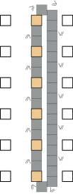
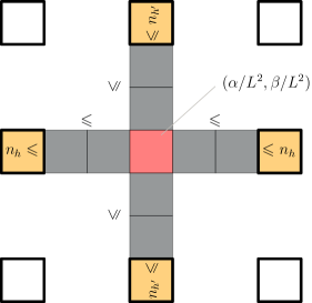
Figure 7: Left: canonical boxes of an equalizer gadget. The offsets are defined so that the indicated inequalities are realized. Right: canonical boxes of an edge check gadget, with offsets along $x_{1}$ and $x_{2}$ corresponding to edges between the partition classes to which $h$ and $h^{\prime}$ are mapped to.

Given our construction for the wiring from above, for each wire we can introduce the offsets within each tuple so that the desired inequality is carried through. Furthermore, we make sure that the start and end of each wire is adjusted so that it can connect to the equalizer and edge check gadgets, as detailed below.

The equalizer gadget relies on carrying an inequality along a cycle, see Figure 7 for a $3$-dimensional example, where the view is from $x_{3}=\infty$. The tuples that connect to the individual wires are drawn in orange. Notice that the offsets introduced on the $x_{3}$ coordinate for the orange boxes must correspond to the type of inequality that the wire carries.

The edge check gadget is again a simple construction, where the middle of the cross is a tuple containing $O(n^{2})$ boxes, where each box is associated with an edge $e$ between the corresponding partition classes $A_{k}$ and $A_{\ell}$. Such edges can be encoded as a subset of $[n]^{2}$, i.e., we have a box $\alpha,\beta$ in the tuple if and only if vertex $\alpha$ of $A_{k}$ is connected to vertex $\beta$ of $A_{\ell}$. The offset for box $(\alpha,\beta)$ compared to the canonical box in the brick is simply $(0,\alpha/L^{2},\beta/L^{2})$.

This concludes the construction. Notice that the construction has an independent set containing exactly one box from each box tuple if and only if $H$ is a subgraph of $G$. The number of tuples needed for the equalizer and edge check gadgets is insignificant compared to those needed in the wiring, which is $\Theta(|V(\mathcal{C})|)=\Theta(k)=\Theta(\bar{k}^{\frac{d}{d-1}}/\alpha^{\frac{d}{d-1}})$. Consequently, the construction has $k=\Theta(\bar{k}^{\frac{d}{d-1}}/\alpha^{\frac{d}{d-1}})$ box tuples, as required.

The final instance has size $n=O(\bar{n}k)+O(\bar{k}\bar{n}^{2})=O(\bar{n}^{3})$. If for all $\gamma>0$ there is an algorithm for packing with running time $n^{\gamma k^{1-1/d}\alpha}$, then we also have algorithms for Partitioned Subgraph Isomorphism with running time

$$n^{\gamma k^{1-1/d}\alpha/\log k)}=\exp\left((\log\bar{n})\cdot\gamma^{\prime}\left(\bar{k}^{\frac{d}{d-1}}/\alpha^{\frac{d}{d-1}}\right)^{1-1/d}\alpha/\log\bar{k})\right)=\bar{n}^{\gamma^{\prime\prime}\cdot\bar{k}/\log\bar{k}}$$

for all $\gamma^{\prime\prime}>0$, which would contradict ETH.

7 Conclusion

We have explored the impact of the stabbing number on the complexity of packing. We have seen that subexponential packing algorithms are possible for similarly sized objects if the stabbing number is $o(n^{1/d})$. The subexponential algorithms could be derived from powerful separator theorems, while the lower bounds required custom wiring results and non-trivial geometric gadgetry. We propose two open problems for future research.

• What is the precise impact of the stabbing number on the complexity of packing if objects are not similarly sized? One can get a subexponential algorithm by an adaptation of the separator in [9], but it yields an algorithm whose dependence on $\alpha$ is much weaker: it has $\alpha^{d}$ in the exponent instead of $\alpha$. Is this algorithm optimal?

• Is there a subexponential algorithm for the Dominating Set problem in intersection graphs of $\alpha$-stabbed similarly sized objects? Or even for $n$ axis-parallel $1\times n^{\varepsilon}$ and $n^{\varepsilon}\times 1$ boxes in two dimensions?

References

- [1] Miklós Abért. Symmetric groups as products of abelian subgroups. Bulletin of the London Mathematical Society, 34(4):451–456, 2002.
- [2] Yohji Akama and Kei Irie. VC dimension of ellipsoids. CoRR, abs/1109.4347, 2011. arXiv:1109.4347.
- [3] Jochen Alber and Jirí Fiala. Geometric separation and exact solutions for the parameterized independent set problem on disk graphs. Journal of Algorithms, 52(2):134–151, 2004. doi:10.1016/j.jalgor.2003.10.001.
- [4] Julien Baste and Dimitrios M. Thilikos. Contraction-bidimensionality of geometric intersection graphs. In IPEC 2017, volume 89 of LIPIcs, pages 5:1–5:13, 2018. doi:10.4230/LIPIcs.IPEC.2017.5.
- [5] Csaba Biró, Édouard Bonnet, Dániel Marx, Tillmann Miltzow, and Paweł Rzążewski. Fine-grained complexity of coloring unit disks and balls. JoCG, 9(2):47–80, 2018. doi:10.20382/jocg.v9i2a4.
- [6] Timothy M. Chan. Polynomial-time approximation schemes for packing and piercing fat objects. J. Algorithms, 46(2):178–189, 2003. doi:10.1016/S0196-6774(02)00294-8.
- [7] Miroslav Chlebík and Janka Chlebíková. Approximation hardness of optimization problems in intersection graphs of d-dimensional boxes. In Proceedings of SODA 2005, pages 267–276. SIAM, 2005. URL: http://dl.acm.org/citation.cfm?id=1070432.1070470.
- [8] Marek Cygan, Fedor V Fomin, Łukasz Kowalik, Daniel Lokshtanov, Dániel Marx, Marcin Pilipczuk, Michał Pilipczuk, and Saket Saurabh. Parameterized Algorithms. Springer, 2015.
- [9] Mark de Berg, Hans L. Bodlaender, Sándor Kisfaludi-Bak, Dániel Marx, and Tom C. van der Zanden. A framework for ETH-tight algorithms and lower bounds in geometric intersection graphs. In Proceedings of STOC 2018, pages 574–586, 2018. doi:10.1145/3188745.3188854.
- [10] Mark de Berg, Hans L. Bodlaender, Sándor Kisfaludi-Bak, Dániel Marx, and Tom C. van der Zanden. A framework for ETH-tight algorithms and lower bounds in geometric intersection graphs. CoRR, abs/1803.10633, 2018. arXiv:1803.10633.
- [11] Erik D. Demaine, Fedor V. Fomin, Mohammad Taghi Hajiaghayi, and Dimitrios M. Thilikos. Fixed-parameter algorithms for -Center in planar graphs and map graphs. ACM Transactions on Algorithms, 1(1):33–47, 2005.
- [12] Erik D. Demaine, Fedor V. Fomin, Mohammad Taghi Hajiaghayi, and Dimitrios M. Thilikos. Subexponential parameterized algorithms on bounded-genus graphs and -minor-free graphs. Journal of the ACM, 52(6):866–893, 2005. doi:10.1145/1101821.1101823.
- [13] Frederic Dorn, Fedor V. Fomin, and Dimitrios M. Thilikos. Subexponential parameterized algorithms. Computer Science Review, 2(1):29–39, 2008.
- [14] Frederic Dorn, Fedor V. Fomin, and Dimitrios M. Thilikos. Catalan structures and dynamic programming in -minor-free graphs. J. Comput. Syst. Sci., 78(5):1606–1622, 2012.
- [15] Frederic Dorn, Eelko Penninkx, Hans L. Bodlaender, and Fedor V. Fomin. Efficient exact algorithms on planar graphs: Exploiting sphere cut decompositions. Algorithmica, 58(3):790–810, 2010.
- [16] Fedor V. Fomin, Daniel Lokshtanov, Venkatesh Raman, and Saket Saurabh. Subexponential algorithms for partial cover problems. Inf. Process. Lett., 111(16):814–818, 2011.
- [17] Fedor V. Fomin, Daniel Lokshtanov, and Saket Saurabh. Bidimensionality and geometric graphs. In Proceedings of SODA 2012, pages 1563–1575. SIAM, 2012. URL: http://portal.acm.org/citation.cfm?id=2095240&CFID=63838676&CFTOKEN=79617016.
- [18] Fedor V. Fomin and Dimitrios M. Thilikos. Dominating sets in planar graphs: Branch-width and exponential speed-up. SIAM J. Comput., 36(2):281–309, 2006.
- [19] Sariel Har-Peled and Kent Quanrud. Approximation algorithms for polynomial-expansion and low-density graphs. SIAM J. Comput., 46(6):1712–1744, 2017. doi:10.1137/16M1079336.
- [20] David Haussler and Emo Welzl. -nets and simplex range queries. Discrete & Computational Geometry, 2(2):127–151, Jun 1987. doi:10.1007/BF02187876.
- [21] Russell Impagliazzo and Ramamohan Paturi. On the complexity of -SAT. Journal of Computer and System Sciences, 62(2):367–375, 2001. doi:10.1006/jcss.2000.1727.
- [22] Fritz John. Extremum Problems with Inequalities as Subsidiary Conditions, pages 197–215. Springer Basel, Basel, 2014. doi:10.1007/978-3-0348-0439-4_9.
- [23] Philip N. Klein and Dániel Marx. A subexponential parameterized algorithm for Subset TSP on planar graphs. In SODA 2014 Proc., pages 1812–1830, 2014.
- [24] Dániel Marx. Can you beat treewidth? Theory of Computing, 6(1):85–112, 2010. doi:10.4086/toc.2010.v006a005.
- [25] Dániel Marx and Michal Pilipczuk. Optimal parameterized algorithms for planar facility location problems using Voronoi diagrams. In Proceedings of ESA 2015, volume 9294 of LNCS, pages 865–877. Springer, 2015. doi:10.1007/978-3-662-48350-3_72.
- [26] Dániel Marx and Anastasios Sidiropoulos. The limited blessing of low dimensionality: when is the best possible exponent for -dimensional geometric problems. In Proceedings of SoCG 2014, pages 67–76. ACM, 2014. doi:10.1145/2582112.2582124.
- [27] Gary L. Miller, Shang-Hua Teng, William P. Thurston, and Stephen A. Vavasis. Separators for sphere-packings and nearest neighbor graphs. J. ACM, 44(1):1–29, 1997. doi:10.1145/256292.256294.
- [28] Marcin Pilipczuk, Michał Pilipczuk, Piotr Sankowski, and Erik Jan van Leeuwen. Subexponential-time parameterized algorithm for Steiner Tree on planar graphs. In STACS 2013 Proc., pages 353–364, 2013.
- [29] Warren D. Smith and Nicholas C. Wormald. Geometric separator theorems & applications. In Proceedings of the 39th Annual Symposium on Foundations of Computer Science, FOCS 1998, pages 232–243. IEEE Computer Society, 1998. doi:10.1109/SFCS.1998.743449.
- [30] Dimitrios M. Thilikos. Fast sub-exponential algorithms and compactness in planar graphs. In ESA 2011 Proc., pages 358–369, 2011.
- [31] A. Frank van der Stappen, Dan Halperin, and Mark H. Overmars. The complexity of the free space for a robot moving amidst fat obstacles. Comput. Geom., 3:353–373, 1993. doi:10.1016/0925-7721(93)90007-S.