Dimensionwise Separable 2-D Graph Convolution for Unsupervised and Semi-Supervised Learning on Graphs

Abstract.

Graph convolutional neural networks (GCN) have been the model of choice for graph representation learning, which is mainly due to the effective design of graph convolution that computes the representation of a node by aggregating those of its neighbors. However, existing GCN variants commonly use 1-D graph convolution that solely operates on the object link graph without exploring informative relational information among object attributes. This significantly limits their modeling capability and may lead to inferior performance on noisy and sparse real-world networks. In this paper, we explore 2-D graph convolution to jointly model object links and attribute relations for graph representation learning. Specifically, we propose a computationally efficient dimensionwise separable 2-D graph convolution (DSGC) for filtering node features. Theoretically, we show that DSGC can reduce intra-class variance of node features on both the object dimension and the attribute dimension to learn more effective representations. Empirically, we demonstrate that by modeling attribute relations, DSGC achieves significant performance gain over state-of-the-art methods for node classification and clustering on a variety of real-world networks. The source code for reproducing the experimental results is available at https://github.com/liqimai/DSGC.

1. Introduction

Graph-structured data occurs in citation networks (Yang et al., 2015), social networks (Ye et al., 2018), traffic networks(Wu et al., [n.d.]), protein networks(Hamilton et al., 2017), knowledge graphs (Wang et al., 2020; Pei et al., [n.d.]) and many other application fields. Analyzing graph data often leads to new insights and interesting discoveries. For example, unsupervised learning on graphs enables to detect user communities in social networks, while semi-supervised learning on graphs helps to predict protein functions in protein networks. Learning effective node representations by utilizing graph structures and other aspects of information such as node content has proved very useful for unsupervised and semi-supervised learning on graphs.

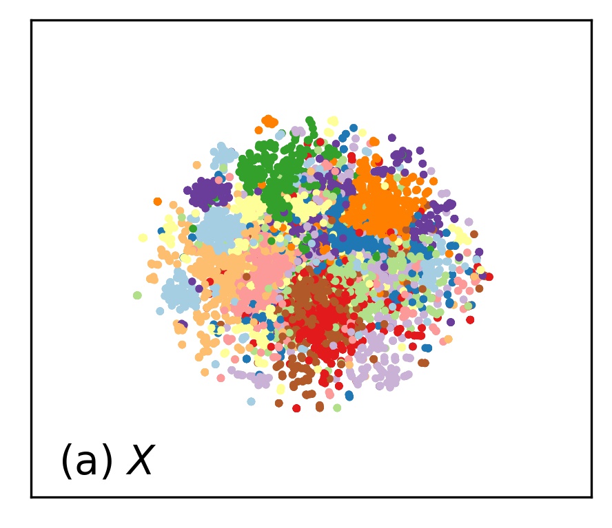
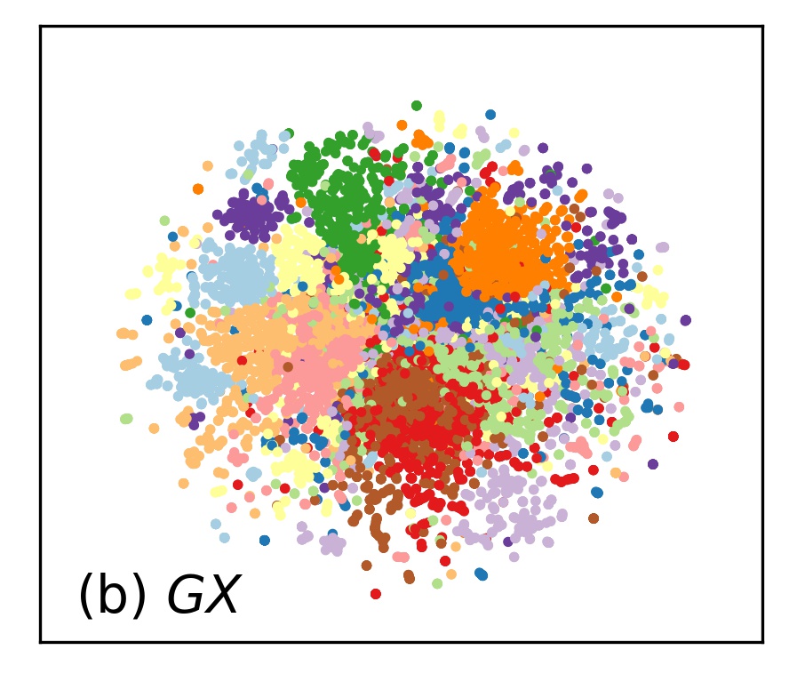
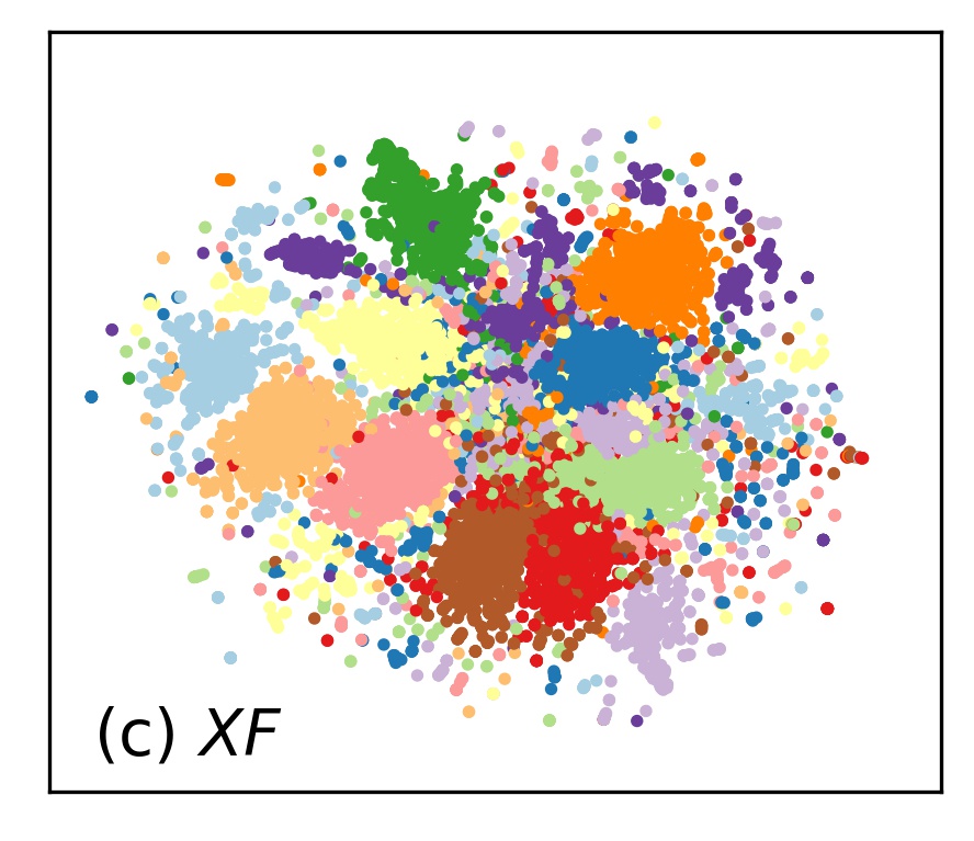
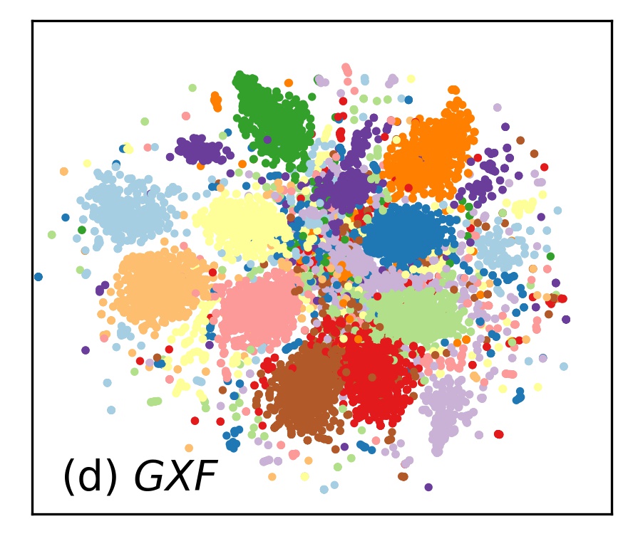
Figure 1. t-SNE visualization of the “20 Newsgroups” dataset. (a) Raw features; (b) Filtered by the regular object graph convolution; (c) Filtered by our proposed attribute graph convolution; (d) Filtered by our proposed dimensionwise separable graph convolution (DSGC).

Previous approaches for unsupervised learning have explored applying non-negative matrix factorization, random walk statistics, and Laplacian eigenmaps on both graph structures and node attributes (Pan et al., 2016; Huang et al., 2017) to learn node representations. For semi-supervised learning, a common way is to regularize a supervised classifier trained with node features by a Laplacian regularizer or an embedding-based regularizer to take into account graph structures, e.g., manifold regularization (Belkin et al., 2006), manifold denoising (Hein and Maier, 2007), deep semi-supervised embedding (Weston et al., 2008), and Planetoid (Yang et al., 2016). However, these methods model node connectivity and node content separately and hence may not be able to fully utilize these information.

In the past few years, graph convolutional neural networks (GCN) and variants have dominated the research of graph representation learning and achieved new state-of-the-art results in various learning tasks on graphs, especially in unsupervised learning (Wang et al., 2017; Zhang et al., 2019) and semi-supervised learning (Kipf and Welling, 2017; Hamilton et al., 2017; Velickovic et al., 2018; Li et al., 2019). The success is mainly attributed to graph convolution, a function that naturally combines node connectivity and node content for feature propagation and smoothing, which computes the representation of a node by aggregating the features of its neighbors. The effective utilization of both modalities of data gives the unique advantage to GCN-based methods over previous approaches, including topology-only models (Perozzi et al., 2014; Grover and Leskovec, 2016) and graph regularization based methods (Belkin et al., 2006; Yang et al., 2016).

In spite of their empirical success, one major limitation of most existing GCN-based methods is that they commonly adopt one-dimensional (1-D) graph convolution that operates on the object link graph to model node (object) relations and features, whose performance critically relies on the quality of the graph. However, real-life networks are often noisy and sparse. For example, in a web graph such as Wikipedia, a hyperlink between two webpages does not necessarily indicate that they belong to the same category, and mixing their features could be harmful for webpage classification or clustering. Moreover, it has been shown that many real-world networks are scale-free and there exist many low-degree nodes (Albert and Barabási, 2002). Since these nodes may have very few or even no links to other nodes, it is difficult, and even impossible, to do feature propagation to endow them with similar features as other same-class nodes to facilitate downstream learning tasks.

To address the above limitation, we propose to explore data relations in another dimension, by constructing an attribute affinity graph, which encodes relations between object attributes. The underlying assumption is attributes that indicate the same category should have strong relations. For example, in a citation network, object attributes are words, and documents of AI category usually contain words such as “learning”, “robotics”, “machine”, “neural”, etc. These indicative words for AI category should be more closely related than other non-indicative words. These informative relations can then be utilized for feature smoothing, similar to the use of object links. Importantly, the attribute affinity graph can be a useful complement to the object link graph in learning node representations. For instance, consider a document that has no links to others (e.g., node e or d in Figure 2), and hence it is impossible to do feature propagation with object links. Yet, with meaningful attribute relations, feature propagation can still be performed along the attribute dimension, and it is possible to obtain similar features for same-class documents.

To formalize the above insight, we propose to perform graph convolution on the attribute affinity graph (Figure 1 (c)). Further, we develop an efficient two-dimensional (2-D) graph convolution to perform feature smoothing on both the object link graph and the attribute affinity graph to learn more effective node representations (Figure 1 (d)). Our main contributions are described as follows.

• Methodology: We propose to use 2-D graph convolution to jointly model object links, attribute relations, and object features for node representation learning. Furthermore, we develop a computationally efficient dimensionwise separable 2-D graph convolutional filter (DSGC), which is equivalent to performing 1-D graph convolution alternately on the object dimension and the attribute dimension, as illustrated in Figure 2. Finally, we propose two learning frameworks based on DSGC for unsupervised node clustering and semi-supervised node classification.

• Theoretical insight: We show that the regular 1-D graph convolution on the object link graph can reduce intra-class variance of node features, which helps to explain the success of many existing methods. Further, we show that the same can be proved for graph convolution on a properly constructed attribute affinity graph. Jointly, they provide a theoretical justification of DSGC.

• Empirical study: We implement DSGC for semi-supervised node classification and unsupervised node clustering, and conduct extensive experiment on a variety of real-world networks including email networks, citation networks, and web graphs. The comparison with state-of-the-art methods demonstrate the advantages of DSGC over the regular 1-D graph convolution. Moreover, we show that DSGC can be easily plugged into some strong GCN-based methods to further improve their performance substantially.

2. Related Works

In this work, we focus on the studies of graph convolutional neural networks for unsupervised and semi-supervised learning. There are a large number of prior works for unsupervised and semi-supervised learning on graph-structured data. We can only briefly review a small portion of them due to space limitation. We first review non-GCN-based methods, then review GCN-based methods.

Network Embedding emerges as an effective way for learning node representations in recent years by leveraging different techniques, such as Markov random walks (Perozzi et al., 2014), matrix factorization (Yang et al., 2015), autoencoders (Cao et al., 2016), and generative adversarial nets (Dai et al., 2018). The learned node representations can boost various downstream learning tasks, such as node clustering (Wang et al., 2016) and node classification (Perozzi et al., 2014).

Graph-based Semi-supervised Learning. Early works in this line explicitly or implicitly adopt the assumption that nearby vertices are likely to have the same label. The most popular framework is label propagation (Zhu et al., 2003; Zhou et al., 2004; Chapelle and Zien, 2005; Wu et al., 2012), which formulates a quadratic regularization framework to implement the cluster assumption and enforce the consistency with labeled data. Other ideas include using graph partition techniques to place the cuts in low density regions (Blum et al., 2004), using spectral kernels to learn smooth low-dimensional embeddings (Chapelle et al., 2003; Zhang and Ando, 2006), and modified adsorption (Talukdar and Crammer, 2009) and iterative classification algorithm (Sen et al., 2008). It was shown in (Ekambaram et al., 2013) and (Girault et al., 2014) that the graph regularization in many of these methods can be interpreted as low-pass graph filters. However, these methods are limited in their ability to incorporate vertex features for prediction. To jointly model graph structures and vertex features, many methods adopt an idea to regularize a supervised learner (e.g., support vector machines, neural networks) with some regularizer such as a Laplacian regularizer or an embedding-based regularizer. Examples include manifold regularization (LapSVM) (Belkin et al., 2006), deep semi-supervised embedding (Weston et al., 2008), and Planetoid (Yang et al., 2016).

Graph Convolutional Neural Networks. In the past few years, a series of works based on graph convolutional neural networks (Li et al., 2016; Qu et al., 2019) have demonstrated promising performance in both semi-supervised and unsupervised learning.

Semi-supervised learning. The pioneering work ChebyNet (Defferrard et al., 2016) exploits a $k$-th order polynomial filter via Chebyshev expansion to avoid the expensive eigen-decomposition in spectral graph convolution. GCN (Kipf and Welling, 2017) simplifies ChebyNet by designing an efficient layer-wise propagation rule with a first-order approximation, which inspires many follow-up works. Specifically, graph attention networks (Velickovic et al., 2018) and gated attention networks (Zhang et al., 2018) introduce attention mechanisms to assign different weights to different nodes in a neighborhood. Some researches (Li et al., 2018) provide deeper insights into GCN by showing the Laplacian smoothing nature and low-pass filtering nature of GCN-like models from spatial and spectral views, respectively. Instead of using two hops of neighbors, some later works such as JKNet (Xu et al., 2018), LanczosNet (Liao et al., 2019), MixHop (Abu-El-Haija et al., 2019), and GCNII (Chen et al., 2020) propose to utilize multiple hops of neighbors.

Unsupervised Learning. One kind of methods stack several graph convolutional layers and learn node representations based on feature/structure preserving, e.g., graph autoencoder and graph variational autoencoder (Kipf and Welling, 2016), GraphSAGE (Hamilton et al., 2017), marginalized graph autoencoder (Wang et al., 2017). Since these methods lack additional constraints to enhance the robustness of representations, adversarially regularized (variational) graph autoencoder (Pan et al., 2018) further adopts GAN to match the learned embeddings with a Gaussian prior. Another type of methods exploit contrastive learning to train an encoder to be contrastive between similar nodes and dissimilar ones for node representation learning, e.g., deep graph infomax (Velickovic et al., 2019) and graphical mutual information (Peng et al., 2020).

However, existing GCN-based methods mainly concentrate on 1-D graph convolution. To our knowledge, the only exception is (Monti et al., [n.d.]), which explores 2-D graph convolution for matrix completion for recommendation. In this work, we investigate 2-D graph convolution for unsupervised and semi-supervised learning.

3. 2-D Graph Convolution

Graph signal processing is an active research field in recent years, which generalizes basic concepts in harmonic analysis, including signals, filters, Fourier transform, and convolution, to the graph domain. Given a graph $\mathcal{G}$ with a vertex set $\mathcal{V}$ and an adjacency matrix $\bm{A}$, if we associate each vertex $\nu_{i}$ with a real value $x_{i}$, then a signal on $\mathcal{G}$ can be defined as a vector $\bm{x}=[x_{i}]$. Graph filters are defined as mappings between input and output signals. Let $\bm{G}$ be a polynomial of $\bm{A}$ (usually normalized), i.e, $\bm{G}=p(\bm{A})$, then $\bm{G}$ is a legit convolutional filter on graph $\mathcal{G}$, and the corresponding 1-D graph convolution is defined as

(1) $$\bm{z}=\bm{G}\bm{x},$$

where $\bm{z}$ is the output signal. Existing graph convolutional filters are all defined in this way and have achieved considerable success in various learning tasks on graphs.

However, previous research mainly focuses on the design and application of 1-D graph convolution. In this section, we present 2-D graph convolution for learning node representations. A comprehensive introduction to multi-dimensional graph convolution is provided by (Kurokawa et al., 2017). Based on the theory developed by (Kurokawa et al., 2017), we propose a localized 2-D graph convolution to circumvent the computationally intensive graph Fourier transform. Furthermore, we propose an even simpler dimensionwise separable 2-D graph convolution to efficiently model both object links and attribute relations.

3.1. 2-D Graph Signal and Spectral Convolution

2-D Graph Signal. A 2-D graph signal is a function defined on the Cartesian product of the vertex sets of two graphs. Formally, given two graphs ${\mathcal{G}}^{(1)}$ and ${\mathcal{G}}^{(2)}$ with $n$ and $m$ nodes respectively, and denote the vertex sets by ${\mathcal{\bm{V}}}^{(1)}$ and ${\mathcal{\bm{V}}}^{(2)}$. A real-valued signal defined on them is a function $x:{\mathcal{\bm{V}}}^{(1)}\times{\mathcal{\bm{V}}}^{(2)}\to\mathbb{R}$. For convenience, we simply denote $x(\nu^{(1)}_{i},\nu^{(2)}_{j})$ by $x_{ij}$ and organize then as a matrix:

(2) $$\bm{X}=(x_{ij})\in\mathbb{\bm{R}}^{n\times m},\quad x_{ij}=x(\nu^{(1)}_{i},\nu^{(2)}_{j}),$$

Signal $\bm{X}$ associates each node pairs $(\nu_{i},\nu_{j})\in\mathcal{V}^{(1)}\times\mathcal{V}^{(2)}$ with a real number $x_{ij}$. For example, the feature matrix given by usual node classification tasks is a 2-D signal defined on object link graph and attribute affinity graph.

2-D Graph Fourier Transform Define the graph Laplacian of ${\mathcal{G}}^{(1)}$ and ${\mathcal{G}}^{(2)}$ as $\bm{L}_{(1)}=\bm{D}^{(1)}-\bm{A}^{(1)}$ and $\bm{L}_{(2)}=\bm{D}^{(2)}-\bm{A}^{(2)}$, where $\bm{A}^{(1)}$, $\bm{A}^{(2)}$ are adjacency matrices and $\bm{D}^{(1)}$, $\bm{D}^{(2)}$ are the corresponding degree matrices. Assuming two Laplacian matrices have following eigen-decomposition

(3) $$\bm{L}_{(1)}=\bm{U}\bm{\Lambda}\bm{U}^{-1},\quad\bm{L}_{(2)}=\bm{V}\bm{M}\bm{V}^{-1},$$

where $\bm{\Lambda},\bm{M}$ stores the eigenvalues $\lambda_{i},\mu_{j}$ of two Laplacian matrices in their main diagonals, $\bm{U}=[\bm{u}_{1},\cdots,\bm{u}_{n}]$ and $\bm{V}=[\bm{v}_{1},\cdots,\bm{v}_{m}]$ store the corresponding unit-length eigen-vectors in their columns. This eigen-decomposition is always attainable for undirected graphs and nearly always attainable for directed graphs.

All $n\times m$ outer products $\bm{u}_{i}\bm{v}_{j}^{\top}$ together form a basis for the linear space $\mathbb{R}^{n\times m}$. It is known as 2-D graph Fourier basis – an analogy of the Fourier basis in classical harmonic analysis in graph domain. A 2-D graph signal $\bm{X}$ can be decomposed in this basis with coefficients $s_{ij}$:

(4) $$\bm{X}=\sum\nolimits_{ij}s_{ij}\left(\bm{u}_{i}\bm{v}_{j}^{\top}\right),$$

or in matrix form:

(5) $$\bm{X}=\bm{U}\bm{S}\bm{V}^{\top},\;\text{where}\;\bm{S}=(s_{ij})\in\mathbb{R}^{n\times m}.$$

$\bm{S}$ is called the spectrum or Fourier coefficients of signal $\bm{X}$ and can be obtained by formula

(6) $$\bm{S}=\bm{U}^{-1}\bm{X}(\bm{V}^{-1})^{\top}.$$

Eq. (6) is so-called 2-D graph Fourier transform; Eq. (5) is the corresponding inverse transform.

2-D Spectral Graph Convolution Given above decomposition, now we can manipulate the spectrum of 2-D signals and define 2-D spectral graph convolution. Convolution is an operation that takes a signal as input and outputs another signal. By convolution theorem, convolution is equivalent to scaling entries of the spectrum. Thus, given a signal $X$ with spectrum $S$, a 2-D spectral graph convolution with $X$ as input is defined as:

(7) $$\bm{Z}=\bm{U}(\bm{S}\circ\bm{P})\bm{V}^{\top},$$

where $\bm{P}$ is the spectral kernel (parameters in spectral domain) of this convolution, and ‘$\circ$’ is Hadamard (entry-wise) product.

3.2. Fast Localized 2-D Graph Convolution

Although Eq. (7) well defines 2-D graph convolution, it is often impractical to perform convolution in the spectral domain, due to the high cost of computing the eigenbasis $\bm{U}$, $\bm{V}$ needed for Fourier transform. Similar to what (Defferrard et al., 2016) did to 1-D graph convolution, we propose 2-D spatial graph convolution here to avoid intensive computation. To achieve this goal, we need to parameterize the entries of spectral kernel $\bm{P}$ as a two-variable polynomial $p(\cdot,\cdot)$ of eigenvalues $\lambda,\mu$ such that $P_{ij}=p(\lambda_{i},\mu_{j})$. Denote coefficients of the polynomial by $\bm{\Theta}=(\theta_{k_{1}k_{2}})\in\mathbb{R}^{n\times m}$, then $\bm{P}$ is parameterized as

(8) $$P_{ij}=p(\lambda_{i},\mu_{j})=\sum_{k_{1}=0}^{n-1}\sum_{k_{2}=0}^{m-1}\theta_{k_{1}k_{2}}\lambda^{k_{1}}_{i}\mu^{k_{2}}_{j}.$$

or in matrix form:

(9) $$\bm{P}=\sum_{k_{1}=0}^{n-1}\sum_{k_{2}=0}^{m-1}\theta_{k_{1}k_{2}}\bm{\Lambda}^{k_{1}}\mathds{1}\bm{M}^{k_{2}},$$

where $\mathds{1}$ denotes all-one matrix of shape $n\times m$. Substitute Eq. (9) into Eq. (7) and rearrange it, 2-D graph convolution will become

$$\bm{Z} =\sum\nolimits_{k_{1}k_{2}}\theta_{k_{1}k_{2}}\bm{U}\left(\bm{S}\circ(\bm{\Lambda}^{k_{1}}\mathds{1}\bm{M}^{k_{2}})\right)\bm{V}^{\top}$$

$$=\sum\nolimits_{k_{1}k_{2}}\theta_{k_{1}k_{2}}\bm{U}\bm{\Lambda}^{k_{1}}\left(\bm{S}\circ\mathds{1}\right)\bm{M}^{k_{2}}\bm{V}^{\top}$$

$$=\sum\nolimits_{k_{1}k_{2}}\theta_{k_{1}k_{2}}\left(\bm{U}\bm{\Lambda}^{k_{1}}\bm{U}^{-1}\right)\bm{X}\left(\bm{V}\bm{M}^{k_{2}}\bm{V}^{-1}\right)^{\top}$$

(10) $$=\sum\nolimits_{k_{1}k_{2}}\theta_{k_{1}k_{2}}\bm{L}_{(1)}^{k_{1}}\bm{X}(\bm{L}_{(2)}^{k_{2}})^{\top}$$

Eq. (10) is called 2-D spatial graph convolution, as it manipulates the signal $\bm{X}$ in the spatial domain. Eigen-decomposition of Laplacian and Fourier transformation of $\bm{X}$ is no longer required. Parameters $\bm{\Theta}=(\theta_{k_{1}k_{2}})$ in Eq. (10) are called the (spatial) kernel of this convolution. Similar to (Defferrard et al., 2016), this spatial convolutional filter is localized. Denote by $K_{1}$ and $K_{2}$ the largest exponent of $\bm{L}_{(1)}$ and $\bm{L}_{(2)}$ in the polynomial, i.e., $k_{1}>K_{1}$ or $k_{2}>K_{2}$ implies $\theta_{k_{1}k_{2}}=0$. The convoluted signal $z_{ij}$ of vertex pair $(\nu^{(1)}_{i},\nu^{(2)}_{j})$ only depends on the neighbourhood of $\nu^{(1)}_{i}$ within $K_{1}$ hops and the neighbourhood of $\nu^{(2)}_{j}$ within $K_{2}$ hops, so the filter is said to be $K_{1}$-localized on ${\mathcal{G}}^{(1)}$ and $K_{2}$-localized on ${\mathcal{G}}^{(2)}$, and the kernel $\bm{\Theta}$ is said to be of size $(K_{1}+1)\times(K_{2}+1)$.

3.3. Dimensionwise Separable 2-D Graph Convolution (DSGC)

Although the above spatial graph convolution avoids the computationally expensive Fourier transform, its general form with kernel size $K_{1}\times K_{2}$ still involves at least $K_{1}\times K_{2}$ matrix multiplications. Inspired by the depth-wise separable convolution proposed in (Howard et al., 2017), we streamline spatial graph convolution by restricting the rank of $\bm{\Theta}$ to be one. Consequently, $\bm{\Theta}$ is able to be decomposed as an outer product of two vectors $\bm{\theta}^{(1)}\in\mathbb{R}^{n}$ and $\bm{\theta}^{(2)}\in\mathbb{R}^{m}$, i.e., $\bm{\Theta}=\bm{\theta}^{(1)}\bm{\theta}^{(2)\top}$ and $\theta_{k_{1}k_{2}}=\theta^{(1)}_{k_{1}}\theta^{(2)}_{k_{2}}$. Finally, the 2-D spatial graph convolution in Eq. (10) becomes

(11) $$\bm{Z} =\sum_{k_{1}=0}^{K_{1}}\sum_{k_{2}=0}^{K_{2}}\theta^{(1)}_{k_{1}}\theta^{(2)}_{k_{2}}\bm{L}_{(1)}^{k_{1}}\bm{X}(\bm{L}_{(2)}^{k_{2}})^{\top}$$

(12) $$=\left(\sum_{k_{1}=0}^{K_{1}}\theta^{(1)}_{k_{1}}\bm{L}_{(1)}^{k_{1}}\right)\bm{X}\left(\sum_{k_{2}=0}^{K_{2}}\theta^{(2)}_{k_{2}}\bm{L}_{(2)}^{k_{2}}\right)^{\top}=\bm{G}\bm{X}\bm{F},$$

(13) $$\text{where }\bm{G}=\sum_{k_{1}=0}^{K_{1}}\theta^{(1)}_{k_{1}}\bm{L}_{(1)}^{k_{1}}\text{ and }\bm{F}=\sum_{k_{2}=0}^{K_{2}}\theta^{(2)}_{k_{2}}(\bm{L}_{(2)}^{k_{2}})^{\top}.$$

We refer to Eq. (12) as dimensionwise separable graph convolution (DSGC), $\bm{G}$ as the object graph convolutional filter, and $\bm{F}$ as the attribute graph convolutional filter. The fastest way to compute it only requires $K_{1}+K_{2}$ matrix multiplications, much less than the $K_{1}\times K_{2}$ matrix multiplications needed by a general 2-D spatial graph convolution. Fig. 2 illustrates how $\bm{G}$ and $\bm{F}$ can work together to learn better node representations with DSGC.

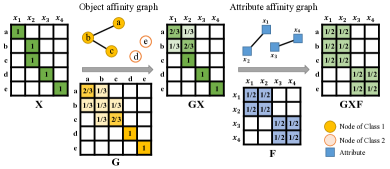
Figure 2. Conceptual illustration of DSGC by a toy example. The node representations (row vectors) obtained by DSGC ($\bm{G}\bm{X}\bm{F}$) is better than those in the originals feature matrix ($\bm{X}$) or filtered by 1-D graph convolution ($\bm{GX}$), in the sense that nodes of the same class have more similar features.

4. Variance Reduction by DSGC

Given a data distribution, the lowest possible error rate an classifier can achieve is the Bayes error rate (Fukunaga, 2013), which is caused by the intrinsic overlap between different classes and cannot be avoided. In this section, we show that DSGC with proper filters can reduce intra-class variance of the data distribution while keeping class centers roughly unchanged, hence reducing the overlap between classes and improving learning performance.

Intra-class Variance and Inter-class Variance Suppose samples $\bm{x}_{i}$ and their labels $y_{i}$ are observations of a random vector $\mathbb{X}=[\mathbb{X}_{1},\cdots,\mathbb{X}_{m}]^{\top}$ and a random variable $\mathbb{Y}$ respectively. We define the variance of random vector $\mathbb{X}$ to be the sum of the variance of each dimension $\mathbb{X}_{j}$, i.e., the trace of the covariance matrix of $\mathbb{X}$. According to law of total variance (Grinstead and Snell, 2012), the variance of $\mathbb{X}$ can be divided into intra-class variance and inter-class variance:

(14) $$\text{Var}\left(\mathbb{X}\right) =\underbrace{\text{E}\left[\text{Var}\left(\mathbb{X}|\mathbb{Y}\right)\right]}_{\text{Intra-class Variance}}+\underbrace{\text{Var}\left(\text{E}\left[\mathbb{X}|\mathbb{Y}\right]\right)}_{\text{Inter-class Variance}},$$

where the conditional variance $\text{Var}\left(\mathbb{X}|\mathbb{Y}=k\right)$ is the variance of class $k$ and the conditional expectation $\text{E}\left[\mathbb{X}|\mathbb{Y}=k\right]$ is the $k$-th class center. Intra-class variance (IntraVar) measures the average divergence within each class, while inter-class variance (InterVar) measures the divergence among class centers. We are interested in the IntraVar$/$InterVar ratio. Desired node representations should have low intra-class variance (i.e., compact and dense for each class), and high inter-classes variance (large margin between classes).

4.1. Intra-class Variance Reduction by Object Graph Convolution

Commonly used object graph convolution reduces variance by averaging over neighborhood. For any node $\nu_{i}$, object graph convolution $\bm{G}\bm{X}$ produces a new feature vector $\bm{z}_{i}=\sum_{j}G_{ij}\bm{x}_{j}$. When $\bm{G}$ is a stochastic matrix, the output feature vector $\bm{z}_{i}$ is a weighted average of the neighbours of $\bm{x}_{i}$. Denote by $\mathbb{Z}$ a random vector of $\bm{z}_{i}$. Intuitively, as long as each node $i$ has enough same-class neighbours, $\mathbb{Z}$ will have a smaller $\text{IntraVar}/\text{InterVar}$ ratio than $\mathbb{X}$.

Formally, assume that objects from different classes are connected with probability $q$, and classes are balanced, i.e., $\Pr(\mathbb{Y}=k)=1/K$ for each class $k$. Then, with the stochastic graph filter $\bm{G}={\bm{D}^{-1}\bm{A}^{(1)}}$, we have the following theorem.

Theorem 1.

When $q$ is sufficiently small, the $\text{IntraVar}/\text{InterVar}$ ratio of $\mathbb{Z}$ is less than or equal to that of $\mathbb{X}$, i.e.,

(15) $$\frac{\text{E}\left[\text{Var}\left(\mathbb{Z}|\mathbb{Y}\right)\right]}{\text{Var}\left(\text{E}\left[\mathbb{Z}|\mathbb{Y}\right]\right)}\leq\frac{\text{E}\left[\text{Var}\left(\mathbb{X}|\mathbb{Y}\right)\right]}{\text{Var}\left(\text{E}\left[\mathbb{X}|\mathbb{Y}\right]\right)}.$$

The proof is given in the Appendices B. This theorem tells that under the assumption that connected nodes are most likely to be of the same class, object graph convolution $\bm{G}\bm{X}$ can efficiently reduce the IntraVar/InterVar ratio.

4.2. Intra-class Variance Reduction by Attribute Graph Convolution

A proper attribute graph convolutional filter $\bm{F}$ can also reduce the IntraVar/InterVar ratio. We use the convention that the random vector $\mathbb{X}$ is a column vector, and hence the attribute graph convolution $\bm{X}\bm{F}$ results in a new random vector $\bm{F}^{\top}\mathbb{X}$. We also assume that the node features are mean-centered, i.e. $\text{E}\left[\mathbb{X}\right]=\bm{0}$.

Theorem 2.

If the attribute graph convolutional filter $\bm{F}$ is a doubly stochastic matrix, then the output of attribute graph convolution has an intra-class variance less than or equal to that of  $\mathbb{X}$, i.e.,

$$\sum\nolimits_{i}F_{ij}=\sum\nolimits_{j} F_{ij}=1\;\text{and}\;F_{ij}\geq 0,\forall\;i,j$$

$$\Rightarrow\quad\text{E}\left[\text{Var}\left(\bm{F}^{\top}\mathbb{X}|\mathbb{Y}\right)\right]\leq\text{E}\left[\text{Var}\left(\mathbb{X}|\mathbb{Y}\right)\right].$$

The proof for Theorem 2 is given in the Appendices C.

To achieve a low IntraVar/InterVar ratio, in addition to reducing intra-class variance, we also need to keep the class centers apart after convolution, which then depends on the quality of the attribute affinity graph. A good attribute affinity graph should connect attributes that share similar expectations conditioned on $\mathbb{Y}$. Formally, each attribute $\mathbb{X}_{j}$ has $K$ conditional expectations w.r.t. $\mathbb{Y}$, which are denoted as a vector $\bm{e}_{j}=(\text{E}\left[\mathbb{X}_{j}|\mathbb{Y}=1\right],\cdots,\text{E}\left[\mathbb{X}_{j}|\mathbb{Y}=K\right])\in\mathbb{R}^{K}$. We have the following.

Theorem 3.

If  $\forall F_{ij}\not=0$, $\left\lVert\bm{e}_{i}-\bm{e}_{j}\right\rVert_{2}\leq\varepsilon$, then the distance between $\bm{e}_{j}$ and $\widehat{\bm{e}}_{j}=\sum_{i}F_{ij}\bm{e}_{i}$ is also less than or equal to $\varepsilon$, i.e.,

$$\left\lVert\bm{e}_{i}-\bm{e}_{j}\right\rVert_{2}\leq\varepsilon,\;\forall F_{ij}\not=0\quad\Rightarrow\quad\left\lVert\bm{e}_{j}-\widehat{\bm{e}}_{j}\right\rVert_{2}\leq\varepsilon,$$

and $\varepsilon$ can be arbitrarily small with a proper $\bm{F}$.

The proof for Theorem 3 is also given in the Appendices C. By Theorem 3, the conditional expectations of each attribute (i.e., class means) may change little after attribute graph convolution, and so does the inter-class variance. Combining Theorems 2 & 3, it suggests that a proper attribute affinity graph should connect attributes that have similar class means, so as to achieve a low $\text{IntraVar}/\text{InterVar}$ ratio and improve performance.

5. Unsupervised and Semi-Supervised Learning with DSGC

5.1. Learning Frameworks

Given an attributed graph with node feature matrix $\bm{X}$, we can learn node representations $\bm{Z}$ in an unsupervised manner by applying DSGC on $\bm{X}$, i.e.,

(16) $$\bm{Z}=\bm{G}\bm{X}\bm{F},$$

and then perform various downstream learning tasks with the node representations $\bm{Z}$.

Unsupervised Node Clustering Any standard clustering algorithm can be applied on $\bm{Z}$ for clustering, as long as it is suitable for present data. In experiments, we use the popular spectral clustering method (Perona and Freeman, 1998; Von Luxburg, 2007) along with linear kernel $\bm{K}=\bm{Z}\bm{Z}^{\top}$.

Semi-supervised Node Classification After obtaining the unsupervised node representations $\bm{Z}$, we may adopt any proper supervised classifier and train it with $\bm{Z}$ and a small portion of labels for semi-supervised classification. This two-step framework is semi-supervised in nature. In experiments, we choose a multi-layer perceptron with a single hidden layer as our classifier. In addition to the two-step framework, we can also plug DSGC into existing end-to-end graph-convolution-based methods. In experiments, we improve several popular methods, including GCN, GAT and GraphSAGE, by replacing their 1-D graph convolution with DSGC. For example, to incorporate DSGC into the vanilla GCN, we can modify the first layer propagation of GCN as:

(17) $$\bm{H}^{(1)}=\sigma(\bm{G}\bm{X}\bm{F}\bm{W}^{(1)}),$$

where $\bm{H}^{(1)}$ is the hidden units in the first layer, $\bm{W}^{(1)}\in\mathbb{R}^{m\times l}$ is the trainable parameters of GCN, and $\sigma$ is an activation function such as ReLU.

Importantly, Eq. (17) can be considered as feeding a filtered feature matrix $\bm{X}\bm{F}$ instead of the raw feature matrix $\bm{X}$ to GCN. By our above analysis, a proper attribute graph convolutional filter $\bm{F}$ can reduce intra-class variance, which makes $\bm{X}\bm{F}$ much easier to classify and guarantees to help train a better model. Furthermore, parameters of GCN is freely chosen from the parameter space $\bm{W}^{(1)}$, while the model trained by Eq. (17) is restricted in a subspace $\bm{F}\bm{W}^{(1)}$. Since the chosen filter $\bm{F}$ is low-pass (Section 5.2) and thus is nearly singular, $\bm{F}\bm{W}^{(1)}$ is a subspace of $\mathbb{R}^{m\times l}$ projected by $\bm{F}$. Model parameters in this subspace are generally better in terms of the generalization performance, due to the variance reduction property of $\bm{F}$. However, the model learned by Eq. (17) can hardly be learned by GCN, since the subspace $\bm{F}\bm{W}^{(1)}$ has measure zero, which is a tiny subset of $\mathbb{R}^{m\times l}$.

Table 1. Dataset statistics.

Dataset	#vertices	#edges	#cls	#features	ratio of intra- class edges
20 NG	18,846	147,034	20	11,697	96.8%
Wiki	3,767	129,597	9	18,316	38.0%
L-Cora	11,881	64,898	10	3,780	76.5%
Corn.	247	384	5	3371	23.7%
Texa.	255	205	5	3371	19.8%
Wisc.	320	721	5	3371	26.3%
Wash.	265	417	5	3371	40.3%

5.2. Implementation of Filters

Object Graph Convolutional Filter In most cases, the object graph $\bm{A}^{(1)}$ is given as part of the dataset, all we need is to design the filter. There are various graph convolutional filters available (Li et al., 2019; Kipf and Welling, 2017; Defferrard et al., 2016; Zhang et al., 2019), but the key principle of filter design for semi-supervised and unsupervised learning is low-pass (Li et al., 2019; NT and Maehara, 2021). Following this principle, we use the 2-order row-normalized affinity matrix as the object graph filter, i.e,

(18) $$\bm{G}=(\bm{I}-\bm{L}_{r}^{(1)})^{2}=(\bm{D}_{1}^{-1}\bm{A}^{(1)})^{2}.$$

Attribute Graph Convolutional Filter A key issue in implementing DSGC is to construct a suitable attribute affinity graph ($\bm{A}^{(2)}$). Possible ways to construct attribute affinity graphs include extracting entity relation information from existing knowledge bases, building a similarity graph from features, or identifying correlations by domain knowledge. In experiments, we evaluate our methods on text dataset as in (Kipf and Welling, 2017; Velickovic et al., 2018; Hamilton et al., 2017), and leverage two suitable attribute affinity graphs for text data described below.

Positive point-wise mutual information (PPMI) is a common tool for measuring the association between two words in computational linguistics (Church and Hanks, 1990). PPMI between words $w_{i}$ and $w_{j}$ is defined by $\text{PPMI}(w_{i},w_{j})=\left[\log\frac{\Pr(w_{i},w_{j})}{\Pr(w_{i})\Pr(w_{j})}\right]_{+}$, where $\Pr(w_{i})$ is the probability of occurrence of word $w_{i}$, and $\Pr(w_{i},w_{j})$ is the probability of two words occurring together. If there is a semantic relation between two words, they usually tend to co-occur more frequently, and thus share a high PPMI value. Here, we use PPMI between words as the corresponding weights in the attribute affinity matrix $A^{(2)}$, and symmetrically normalize it as (Kipf and Welling, 2017).

Word embedding based $k$-NN graphs. Word embedding is a collection of techniques that map vocabularies to vectors in an Euclidean space. Embeddings of words are pre-trained vectors learned from corpus with algorithms such as GloVe (Pennington et al., 2014). Since word embeddings capture semantic relations between words (Bakarov, 2018), they can be used for constructing an attribute affinity graph. With the embedding vectors, we can construct a $k$-NN graph with some proximity metric such as the Euclidean distance.

With the constructed attribute affinity graph ($\bm{A}^{(2)}$), we use one-step lazy random walk filter (Li et al., 2019) in our experiments, i.e.,

(19) $$\bm{F}=(\bm{I}-\frac{1}{2}\bm{L}_{s})=\frac{1}{2}(\bm{I}+\bm{D}_{2}^{-1/2}\bm{A}^{(2)}\bm{D}_{2}^{-1/2}).$$

6. Empirical Study

We conduct extensive experiments in semi-supervised node classification and node clustering on seven real-world networks including 20 Newsgroups (20 NG) (Lang, 1995), Large Cora (L-Cora) (McCallumzy et al., 1999; Li et al., 2019), Wikispeedia (Wiki) (West et al., 2009; West and Leskovec, 2012), and four subsets of WebKB (Cornell, Texas, Wisconsin, and Washington). Due to space limitation, on the four subsets of WebKB, we only report the results of semi-supervised node classification with some representative baselines, but the results are indicative enough.

Figure 3. IntraVar/InterVar ratios. The lower, the better.

Table 2. Classification accuracy on 20 NG, L-Cora, and Wiki.

Dataset			20 NG		L-Cora		Wiki
Method	$\bm{G}$	$\bm{F}$	20 labels/cls.	5 labels/cls.	20 labels/cls.	5 labels/cls.	20 labels/cls.	5 labels/cls.
MLP	✗	✗	63.76 $\pm$ 0.17	38.67 $\pm$ 0.38	52.97 $\pm$ 0.41	39.56 $\pm$ 0.85	67.23 $\pm$ 0.25	54.41 $\pm$ 0.66
LP (Zhu et al., 2003)	✓	✗	16.39 $\pm$ 0.20	8.62 $\pm$ 0.20	55.77 $\pm$ 0.97	38.97 $\pm$ 3.15	9.53 $\pm$ 0.05	10.54 $\pm$ 0.19
GLP (Li et al., 2019)	✓	✗	74.99 $\pm$ 0.11	52.62 $\pm$ 0.45	68.95 $\pm$ 0.29	56.42 $\pm$ 0.85	60.05 $\pm$ 0.11	48.45 $\pm$ 0.54
GCN (Kipf and Welling, 2017)	✓	✗	76.25 $\pm$ 0.11	53.78 $\pm$ 0.49	67.75 $\pm$ 0.33	54.27 $\pm$ 0.82	59.81 $\pm$ 0.30	47.93 $\pm$ 0.56
GAT (Velickovic et al., 2018)	✓	✗	76.33 $\pm$ 0.16	56.02 $\pm$ 0.57	68.88 $\pm$ 0.78	56.89 $\pm$ 1.53	50.97 $\pm$ 0.54	46.99 $\pm$ 0.83
DGI (Velickovic et al., 2019)	✓	✗	73.34 $\pm$ 0.27	66.57 $\pm$ 0.63	61.39 $\pm$ 0.50	54.77 $\pm$ 1.24	49.70 $\pm$ 1.63	43.64 $\pm$ 1.89
GraphSAGE (Hamilton et al., 2017)	✓	✗	65.73 $\pm$ 0.17	42.48 $\pm$ 0.77	57.28 $\pm$ 0.71	46.79 $\pm$ 1.91	65.52 $\pm$ 0.62	48.81 $\pm$ 0.76
GCNII (Chen et al., 2020)	✓	✗	77.41 $\pm$ 0.12	58.10 $\pm$ 0.85	68.18 $\pm$ 0.19	57.02 $\pm$ 0.55	43.65 $\pm$ 1.03	35.98 $\pm$ 4.45
JK-MaxPool (Xu et al., 2018)	✓	✗	71.00 $\pm$ 0.19	49.09 $\pm$ 0.27	67.44 $\pm$ 0.18	51.63 $\pm$ 0.52	45.26 $\pm$ 0.37	44.13 $\pm$ 0.38
JK-Concat (Xu et al., 2018)	✓	✗	72.24 $\pm$ 0.13	49.76 $\pm$ 0.27	67.47 $\pm$ 0.19	51.96 $\pm$ 0.46	47.24 $\pm$ 0.30	45.21 $\pm$ 0.29
GRAND (Feng et al., 2020)	✓	✗	74.45 $\pm$ 0.72	57.97 $\pm$2.79	69.30 $\pm$ 0.59	52.12 $\pm$ 0.73	62.25 $\pm$ 0.93	47.17 $\pm$ 3.38
DSGC ($\bm{G}\bm{X}$)	✓	✗	75.60 $\pm$ 0.13	53.84 $\pm$ 0.46	67.74 $\pm$ 0.30	55.67 $\pm$ 0.72	58.73 $\pm$ 0.34	47.34 $\pm$ 0.54
DSGC ($\bm{X}\bm{F}$)	✗	Emb	66.27 $\pm$ 0.13	48.04 $\pm$ 0.38	58.70 $\pm$ 0.30	46.41 $\pm$ 0.55	69.76 $\pm$ 0.20	59.76 $\pm$ 0.58
	✗	PPMI	75.36 $\pm$ 0.11	59.61 $\pm$ 0.34	61.01 $\pm$ 0.23	48.31 $\pm$ 0.62	69.91 $\pm$ 0.21	60.13 $\pm$ 0.61
DSGC ($\bm{G}\bm{X}\bm{F}$)	✓	Emb	76.53 $\pm$ 0.15	59.91 $\pm$ 0.31	69.81 $\pm$ 0.26	58.63 $\pm$ 0.75	60.50 $\pm$ 0.26	49.69 $\pm$ 0.56
	✓	PPMI	81.69 $\pm$ 0.12	68.94 $\pm$ 0.32	70.20 $\pm$ 0.24	59.43 $\pm$ 0.68	58.84 $\pm$ 0.26	48.51 $\pm$ 0.54
⋆ ✓  and ✗  indicate using/not using $\bm{G}$ or $\bm{F}$.

Table 3. Classification accuracy on four subsets of WebKB.

Method	$\bm{F}$	Corn.	Texa.	Wisc.	Wash.
GCN (Kipf and Welling, 2017)	✗	50.25 $\pm$0.66	60.31 $\pm$1.06	52.74 $\pm$0.92	53.83 $\pm$1.36
GLP (Li et al., 2019)	✗	50.86 $\pm$0.75	59.40 $\pm$1.27	55.28 $\pm$0.97	55.87 $\pm$1.32
GAT (Velickovic et al., 2018)	✗	51.21 $\pm$1.40	60.06 $\pm$1.08	52.92 $\pm$1.18	56.85 $\pm$2.00
GRAND (Feng et al., 2020)	✗	49.01 $\pm$1.04	57.38 $\pm$0.26	49.30 $\pm$0.22	42.09 $\pm$1.25
DSGC ($\bm{G}\bm{X}$)	✗	51.22 $\pm$0.77	59.35 $\pm$1.26	56.26 $\pm$0.93	55.77 $\pm$1.30
DSGC ($\bm{X}\bm{F}$)	Emb	62.14 $\pm$1.02	68.00 $\pm$0.75	73.50 $\pm$0.81	65.78 $\pm$1.27
	PPMI	60.10 $\pm$0.91	67.34 $\pm$0.94	72.88 $\pm$0.78	65.40 $\pm$1.35
DSGC ($\bm{G}\bm{X}\bm{F}$)	Emb	53.02 $\pm$0.67	61.89 $\pm$0.94	58.64 $\pm$1.12	59.05 $\pm$1.21
	PMI	52.35 $\pm$0.52	61.83 $\pm$0.91	56.40 $\pm$1.04	57.01 $\pm$1.20

6.1. Datasets

The statistics of all datasets are summarized in Table 1, where the last row shows the intra-class edge ratio of the object link graph of each dataset, which can reflect the quality of the graph.

20 Newsgroups (20 NG) (Lang, 1995) is an email discussion group, where each object is an email and there are 18846 emails in total. Each email is represented by an 11697-dimension tf-idf feature vector. Two emails are connected by an edge if they replies the same one.

Wikispeedia (Wiki) (West et al., 2009; West and Leskovec, 2012) is a webpage network in which the objects are 3767 Wikipedia webpages, and the edges are web hyperlinks. Each webpage is described by a 18316-dimension tf-idf vector. We removed several tiny classes, so the webpages distribute more evenly across the remaining 9 categories.

Large Cora (L-Cora) (McCallumzy et al., 1999) is a citation network in which the objects are computer science research papers represented by 3780 dimension of tf-idf values. Two papers are connected by an undirected edge if and only if one cites the other. These citation links form a object graph. After removing the papers that belong to no topic and the ones that have no authors or title, a subset of 11881 papers is obtained (Saccá et al., 2013). We name this dataset “Large Cora” to distinguish it from the “Cora” dataset with 2708 papers used in (Kipf and Welling, 2017; Yang et al., 2016; Sen et al., 2008).

WebKB is a webpage dataset collected by Carnegie Mellon University. We use its four subdatasets: Cornell, Texas, Wisconsin, and Washington. The objects are webpages, and the edges are hyperlinks between them. The webpages are represented by tf-idf feature vectors, and manually classified into five categories: student, project, course, staff, and faculty.

6.2. Variance Reduction and Visualization

First of all, to verify our analysis in section 4, we illustrate the variance reduction effect of both object graph convolution and attribute graph convolution. As shown in Figure 3, 1-D graph convolution ($\bm{GX}$ or $\bm{XF}$) already greatly reduces the $\text{IntraVar}/\text{InterVar}$ ratio, and 2-D graph convolution ($\bm{GXF}$) reduces it even further.

In Figure 1, we visualize the results of performing graph convolution on the object features of 20 NG by t-SNE. It can be seen that both object graph convolution and attribute graph convolution can successfully reduce the overlap among classes, and 2-D graph convolution (DSGC) is more effective than 1-D.

6.3. Semi-supervised Node Classification

Table 4. Baselines improved by DSGC.

Methods	$\bm{F}$	20 NG	L-Cora	Wiki
GAT (Velickovic et al., 2018)	✗	76.33 $\pm$ 0.16	68.88 $\pm$ 0.78	50.97 $\pm$ 0.54
	PPMI	78.01 $\pm$ 0.30	67.38 $\pm$ 0.65	55.43 $\pm$ 0.51
GCN (Kipf and Welling, 2017)	✗	76.25 $\pm$ 0.11	67.75 $\pm$ 0.33	59.81 $\pm$ 0.30
	PPMI	81.60 $\pm$ 0.10	67.87 $\pm$ 0.25	61.33 $\pm$ 0.28
GraphSAGE (Hamilton et al., 2017)	✗	65.73 $\pm$ 0.17	57.28 $\pm$ 0.71	65.52 $\pm$ 0.62
	PPMI	76.27 $\pm$ 0.33	60.23 $\pm$ 1.81	67.26 $\pm$ 0.52
⋆ ✗  indicates not using $\bm{F}$.

Baselines We compare DSGC with the following baselines: label propagation (LP) (Wu et al., 2012), multi-layer perceptron (MLP), graph convolutional networks (GCN) (Kipf and Welling, 2017), generalized label propagation (GLP) (Li et al., 2019), GraphSAGE (Hamilton et al., 2017), graph attention networks (GAT) (Velickovic et al., 2018), deep graph infomax (DGI) (Velickovic et al., 2019), GCNII (Chen et al., 2020), jumping knowledge networks (JK-MaxPool & JK-Concat) (Xu et al., 2018), and GRAND(Feng et al., 2020). We also try to improve GCN, GAT, and GraphSAGE by DSGC as described in Section 5.1. Our methods with mere object graph filter ($\bm{G}$) or mere attribute graph filter ($\bm{F}$) are also tested, for the purpose of ablation study. PPMI and Emb denote attribute affinity graphs constructed by positive point-wise mutual information and word embedding respectively as described in Section 5.2).

Table 5. Clustering performance.

Dataset			20 NG		L-Cora		Wiki
Method	$\bm{G}$	$\bm{F}$	Acc(%)	NMI(%)	Acc(%)	NMI(%)	Acc(%)	NMI(%)
Spectral	✗	✗	25.29 $\pm$ 1.01	28.18 $\pm$ 0.74	28.22 $\pm$ 1.01	11.61 $\pm$ 0.04	29.25 $\pm$ 0.00	21.83 $\pm$ 0.00
GAE (Kipf and Welling, 2016)	✓	✗	38.92 $\pm$ 1.39	44.58 $\pm$ 0.40	34.45 $\pm$ 0.76	22.38 $\pm$ 0.18	33.78 $\pm$ 0.32	22.88 $\pm$ 0.20
VGAE (Kipf and Welling, 2016)	✓	✗	25.04 $\pm$ 0.81	25.72 $\pm$ 0.77	29.45 $\pm$ 1.25	17.53 $\pm$ 0.15	33.83 $\pm$ 0.45	21.46 $\pm$ 0.19
MGAE (Wang et al., 2017)	✓	✗	47.83 $\pm$ 2.33	56.14 $\pm$ 1.00	35.87 $\pm$ 0.97	30.57 $\pm$ 0.98	32.73 $\pm$ 1.16	27.95 $\pm$ 2.29
ARGE (Pan et al., 2018)	✓	✗	42.04 $\pm$ 0.50	44.13 $\pm$ 0.91	36.07 $\pm$ 0.05	27.74 $\pm$ 0.01	26.49 $\pm$ 0.10	17.17 $\pm$ 0.05
ARVGE (Pan et al., 2018)	✓	✗	21.10 $\pm$ 0.61	21.79 $\pm$ 0.49	26.45 $\pm$ 0.03	12.94 $\pm$ 0.01	33.82 $\pm$ 0.13	21.42 $\pm$ 0.11
AGC (Zhang et al., 2019)	✓	✗	38.83 $\pm$ 0.84	47.08 $\pm$ 1.57	41.76 $\pm$ 0.01	33.65 $\pm$ 0.01	32.74 $\pm$ 0.01	24.90 $\pm$ 0.01
DSGC ($\bm{G}\bm{X}$)	✓	✗	38.42 $\pm$ 0.66	46.28 $\pm$ 0.93	38.26 $\pm$ 0.02	30.66 $\pm$ 0.02	31.43 $\pm$ 0.09	24.16 $\pm$ 0.18
DSGC ($\bm{X}\bm{F}$)	✗	Emb	28.99 $\pm$ 0.06	33.22 $\pm$ 0.10	30.80 $\pm$ 0.56	17.46 $\pm$ 0.21	35.45 $\pm$ 0.91	33.44 $\pm$ 0.66
	✗	PPMI	48.36 $\pm$ 2.40	53.27 $\pm$ 2.17	36.46 $\pm$ 0.06	22.53 $\pm$ 0.03	38.10 $\pm$ 0.01	36.07 $\pm$ 0.02
DSGC ($\bm{G}\bm{X}\bm{F}$)	✓	Emb	43.40 $\pm$ 0.66	50.97 $\pm$ 0.58	40.75 $\pm$ 0.02	33.05 $\pm$ 0.04	30.50 $\pm$ 0.01	25.48 $\pm$ 0.03
	✓	PPMI	52.25 $\pm$ 1.97	61.34 $\pm$ 1.07	41.24 $\pm$ 0.04	30.92 $\pm$ 0.01	31.37 $\pm$ 0.08	26.06 $\pm$ 0.20
⋆ ✓  and ✗  indicate using/not using $\bm{G}$ or $\bm{F}$.

Settings For 20 NG, L-Cora and Wiki, we test two scenarios – 20 labels/class and 5 labels/class. We follow GCN (Kipf and Welling, 2017) and many others to set aside a validation set containing 500 samples for hyper-parameter tuning. For the four small subdatasets of WebKB, we randomly split them into 5/30/65% as train/valid/test set, and ensure each class has at least 1 label. Hyper-parameters of all methods, including ours and baselines, are tuned by grid search according to validation. The reported results of all methods are averaged over 50 runs. More experimental details are provided in Appendix A.

Performance Classification accuracies are summarized in Tables 2 and  3, and the top 2 accuracies are highlighted. Results of improved GAT, GCN, and GraphSAGE are shown in Table 4. The following observations can be made. Firstly, object graph convolution ($\bm{G}$) does not always help. On 20 NG and L-Cora, methods based on it like DSGC ($\bm{GX}$), GCN and GAT all outperform MLP significantly. However, on Wiki and the four subsets of WebKB, object graph convolution severely harms the performance. This is because the hyperlink graphs are highly noisy. Only a small portion of edges connect nodes of the same class, much lower than that of 20 NG (96.8%) and L-Cora (76.5%) (see Table 1). This shows the limitation of object graph convolution. Secondly, attribute graph convolution works. As shown in Table 2, DSGC with mere $\bm{F}$ already outperforms MLP significantly. Especially, on Wiki and WebKB, object graph convolution fails while attribute graph convolution is still effective. Thirdly, 2-D graph convolution is useful. On datasets with good object link graphs like 20 NG and L-Cora, DSGC with both $\bm{G}$ and $\bm{F}$ performs much better than with either one of them only. Especially, DSGC ($\bm{G}\bm{X}\bm{F}$) with PPMI achieves the best performance among all methods. On datasets with bad object link graphs such as Wiki and the four subsets of WebKB, DSGC with both $\bm{G}$ and $\bm{F}$ improves upon DSGC with mere $\bm{G}$ and outperforms most baselines. Especially, DSGC with mere $\bm{F}$ achieves the best performance, which improves upon the best baseline by 3.63% and 5.72% in absolute accuracy in two scenarios.

Remarkably, it can be seen from Table 4 that by incorporating DSGC, the performance of baselines including GCN, GAT, GraphSAGE is improved substantially in most cases, which again confirms that attribute graph convolution is a useful complement to object graph convolution.

6.4. Node Clustering

Baselines We test the proposed node clustering method with DSGC (Section 5.1) with or without $\bm{G}$ and $\bm{F}$ in five cases, and compare them with existing strong baselines including GAE and VGAE (Kipf and Welling, 2016), MGAE (Wang et al., 2017), ARGE and ARVGE (Pan et al., 2018) and AGC (Zhang et al., 2019). We also compare with the spectral clustering (Spectral) method that operates on a similarity graph constructed by a linear kernel. Detailed experiment settings are included in Appendix A.

Performance We adopt two widely-used clustering measures (Aggarwal and Reddy, 2014): clustering accuracy (Acc) and normalized mutual information (NMI), and the results are shown in Table 5 with the top 2 results highlighted. We can make the following observations. 1) Attribute graph convolution is highly effective. On 20 NG, DSGC ($\bm{X}\bm{F}$) with PPMI outperforms most baselines by a very large margin. On Wiki, DSGC ($\bm{X}\bm{F}$) with PPMI or Emb significantly outperforms all the baselines. 2) 2-D graph convolution is beneficial as validated in the classification experiments. On 20 NG, DSGC ($\bm{GXF}$) with PPMI can further improve upon the already very strong performance of DSGC ($\bm{X}\bm{F}$) with PPMI and performs the best; On L-Cora, DSGC ($\bm{GXF}$) with PPMI or Emb improves upon either DSGC ($\bm{G}\bm{X}$) or DSGC ($\bm{X}\bm{F}$) and outperforms most baselines significantly. On Wiki, DSGC ($\bm{X}\bm{F}$) performs better than DSGC ($\bm{GXF}$), due to the low-quality object link graph as explained above.

7. Conclusion

We have proposed a simple and efficient dimensionwise separable 2-D graph convolution (DSGC) for unsupervised and semi-supervised learning on graphs. We have demonstrated theoretically and empirically that by exploiting attribute relations in addition to object relations, DSGC can learn better node representations than existing methods based on the regular 1-D graph convolution, leading to promising performance on node classification and clustering tasks. We believe DSGC can be applied to a wide variety of applications such as action recognition, malware detection, and recommender systems. In future work, we plan to apply DSGC to solve more practical problems.

Appendix A Experimental Settings

A.1. Semi-supervised Node Classification

For constructing the PPMI graph, we set the context window size to 20 and use the inverse distance as co-occurrence weight. For constructing the Emb graph, we use GloVe (Pennington et al., 2014) to learn word embeddings and set the number of nearest neighbours $k=20$. The classifier of DSGC we use is a multi-layer perceptron (MLP) with a 64-unit hidden layer. The MLP is trained for 200 epochs by Adam Optimizer.

Hyperparameters of all models, including our methods and baselines, are tuned by grid search based on validation. Dropout rate is selected from {0, 0.2, 0.5}, and 0.2 is chosen. Learning rate is selected from {1, 0.1, 0.01, 0.001}, and 0.1 is chosen. Weight decay is selected from {5e-3, 5e-4, 5e-5, 5e-6, 5e-7}, and 5e-4 is chosen for WebKB, 5e-5 for L-Cora, 5e-6 for 20 NG, 5e-7 for Wiki. Results of our methods and baselines are averaged over 50 runs.

A.2. Node Clustering

For our method DSGC, the attribute affinity graphs PPMI and Emb are constructed in the same way as in object classification. For other baselines, we follow the parameter settings described in the original papers. In particular, for GAE and VGAE (Kipf and Welling, 2016), we construct encoders with a 32-neuron hidden layer and a 16-neuron embedding layer, and train the encoders for 200 iterations using the Adam algorithm with a learning rate of 0.01.

For MGAE (Wang et al., 2017), the corruption level $p$ is 0.4, the number of layers is 3, and the parameter $\lambda$ is $10^{-5}$. For ARGE and ARVGE (Pan et al., 2018), we construct encoders with a 32-neuron hidden layer and a 16-neuron embedding layer. The discriminators are built by two hidden layers with 16 neurons and 64 neurons respectively. We train all the autoencoder-related models for 200 iterations and optimize them using the Adam algorithm. The learning rates of encoder and discriminator are both 0.001. For AGC (Zhang et al., 2019), the maximum iteration number is 60. For fair comparison, these baselines also adopt spectral clustering as our DSGC to obtain the clustering results. We repeat each method for 10 times and report the average clustering results and standard deviations.

Appendix B

Assume that objects from the same class are connected with probability $r$, and objects from different classes are connected with probability $q$, i.e., the adjacency matrix $\bm{A}^{(1)}$ of object graph obeys following distribution:

	if $y_{i}=y_{j}$	if $y_{i}\not=y_{j}$
$\Pr(a_{ij}\not=0)$	$r$	$q$
$\Pr(a_{ij}=0)$	$1-r$	$1-q$

We also assume that classes are balanced, i.e., $\Pr(\mathbb{Y}=k)=1/K$ for all $k$. Then, with the stochastic graph filter $\bm{G}={\bm{D}^{-1}\bm{A}^{(1)}}$, we have the following theorem.

Theorem 1.

When $q$ is sufficiently small, the $\text{IntraVar}/\text{InterVar}$ ratio of $\mathbb{Z}$ is less than or equal to that of $\mathbb{X}$, i.e.,

(20) $$\frac{\text{E}\left[\text{Var}\left(\mathbb{Z}|\mathbb{Y}\right)\right]}{\text{Var}\left(\text{E}\left[\mathbb{Z}|\mathbb{Y}\right]\right)}\leq\frac{\text{E}\left[\text{Var}\left(\mathbb{X}|\mathbb{Y}\right)\right]}{\text{Var}\left(\text{E}\left[\mathbb{X}|\mathbb{Y}\right]\right)}.$$

Proof.

The proof consists of two parts. In the first part, we prove that inter-class variance is unchanged after object graph convolution, when $q$ approximates 0, i.e.,

(21) $$\lim_{q\to 0}\text{Var}\left(\text{E}\left[\mathbb{Z}|\mathbb{Y}\right]\right)=\text{Var}\left(\text{E}\left[\mathbb{X}|\mathbb{Y}\right]\right).$$

In the second part, we prove that intra-class variance becomes smaller after object graph convolution, i.e.,

(22) $$\text{E}\left[\text{Var}\left(\mathbb{Z}|\mathbb{Y}\right)\right]\leq\text{E}\left[\text{Var}\left(\mathbb{X}|\mathbb{Y}\right)\right],$$

when $G$ is a stochastic matrix.

Part 1. Inter-class variance is unchanged. Since $\bm{z}_{i}=\sum_{j}G_{ij}\bm{x}_{j}$, we have

$$\quad\text{E}\left[\bm{z}_{i}|y_{i}=k\right]=\sum_{j}\text{E}\left[G_{ij}\right]\text{E}\left[\bm{x}_{j}\right]$$

$$=\sum_{j,y_{j}=k}\text{E}\left[G_{ij}\right]\text{E}\left[\bm{x}_{j}\right]+\sum_{j,y_{j}\not=k}\text{E}\left[G_{ij}\right]\text{E}\left[\bm{x}_{j}\right]$$

$$=\frac{\sum_{j,y_{j}=k}\text{E}\left[a_{ij}\right]\text{E}\left[\bm{x}_{j}\right]+\sum_{j,y_{j}\not=k}\text{E}\left[a_{ij}\right]\text{E}\left[\bm{x}_{j}\right]}{\sum_{j}\text{E}\left[a_{ij}\right]}$$

$$=\frac{r\sum_{j,y_{j}=k}\text{E}\left[\mathbb{X}|\mathbb{Y}=k\right]+q\sum_{j,y_{j}\not=k}\text{E}\left[\bm{x}_{j}\right]}{\frac{N}{K}(r-q)+Nq}$$

$$=\frac{\frac{N}{K}r\text{E}\left[\mathbb{X}|\mathbb{Y}=k\right]+q\sum_{j}\text{E}\left[\bm{x}_{j}\right]-q\sum_{j,y_{j}=k}\text{E}\left[\bm{x}_{j}\right]}{\frac{N}{K}(r-q)+Nq}$$

$$=\frac{\frac{N}{K}(r-q)\text{E}\left[\mathbb{X}|\mathbb{Y}=k\right]+Nq\text{E}\left[\mathbb{X}\right]}{\frac{N}{K}(r-q)+Nq}$$

(23) $$=\frac{(r-q)\text{E}\left[\mathbb{X}|\mathbb{Y}=k\right]+Kq\text{E}\left[\mathbb{X}\right]}{(r-q)+Kq}$$

When $q$ approximates $0$, Eq. (23) approximates $\text{E}\left[\mathbb{X}|\mathbb{Y}=k\right]$, so

$$\quad\text{E}\left[\mathbb{Z}|\mathbb{Y}=k\right]=\sum_{i,y_{i}=k}\Pr(\mathbb{Z}=\bm{z}_{i}|y_{i}=k)\text{E}\left[\bm{z}_{i}|y_{i}=k\right]$$

$$=\sum_{i,y_{i}=k}\Pr(\mathbb{Z}=\bm{z}_{i}|y_{i}=k)\text{E}\left[\mathbb{X}|\mathbb{Y}=k\right]=\text{E}\left[\mathbb{X}|\mathbb{Y}=k\right].$$

Take variance of both side, we get

(24) $$\text{Var}\left(\text{E}\left[\mathbb{Z}|\mathbb{Y}\right]\right)=\text{Var}\left(\text{E}\left[\mathbb{X}|\mathbb{Y}\right]\right).$$

Part 2. Intra-class variance becomes smaller. Denote by $\text{Cov}\left(\cdot,\cdot\right)$ the covariance of two random variables. We have following inequality about variance.

$$\text{Var}\left(\sum_{j}G_{ij}\bm{x}_{j}\right) =\sum_{j}G_{ij}^{2}\text{Var}\left(\bm{x}_{j}\right)+\sum_{j,l}G_{ij}G_{il}\text{Cov}\left(\bm{x}_{j},\bm{x}_{l}\right)$$

$$\leq\sum_{j,l}G_{ij}G_{il}\sqrt{\text{Var}\left(\bm{x}_{j}\right)}\sqrt{\text{Var}\left(\bm{x}_{l}\right)}$$

(25) $$=\left(\sum_{j}G_{ij}\sqrt{\text{Var}\left(\bm{x}_{j}\right)}\right)^{2}.$$

Consider the variance of filtering result $\bm{z}_{i}$ for each sample in class $k$, it is less than variance of $\mathbb{X}$ of that class:

$$\quad\text{Var}\left(\bm{z}_{i}|y_{i}=k\right)$$

$$=\text{Var}\left(\left.\sum_{j}G_{ij}\bm{x}_{j}\right|y_{j}=k\right)$$

$$\leq\left(\sum_{j}G_{ij}\sqrt{\text{Var}\left(\bm{x}_{j}|y_{j}=k\right)}\right)^{2}$$ # by inequality (25)

$$=\left(\sum_{j}G_{ij}\sqrt{\text{Var}\left(\mathbb{X}|\mathbb{Y}=k\right)}\right)^{2}$$

$$=\left(\sqrt{\text{Var}\left(\mathbb{X}|\mathbb{Y}=k\right)}\right)^{2} \sum_{j}G_{ij}=1$$ # since

$$=\text{Var}\left(\mathbb{X}|\mathbb{Y}=k\right),$$

Then variance of random vector $\mathbb{Z}$ for each class is less than variance of $\mathbb{X}$ of that class:

$$\text{Var}\left(\mathbb{Z}|\mathbb{Y}=k\right) =\sum_{i,y_{i}=k}\Pr(\mathbb{Z}=\bm{z}_{i}|y_{i}=k)\text{Var}\left(\bm{z}_{i}|y_{i}=k\right)$$

$$\leq\text{Var}\left(\mathbb{X}|\mathbb{Y}=k\right).$$

Sum tham over all classes:

$$\qquad\text{E}\left[\text{Var}\left(\mathbb{Z}|\mathbb{Y}\right)\right] =\sum_{k}\Pr(\mathbb{Y}=k)\text{Var}\left(\mathbb{Z}|\mathbb{Y}=k\right)$$

$$\leq\sum_{k}\Pr(\mathbb{Y}=k)\text{Var}\left(\mathbb{X}|\mathbb{Y}=k\right)$$

(26) $$=\text{E}\left[\text{Var}\left(\mathbb{X}|\mathbb{Y}\right)\right].$$

Combining Eq. (24) and Eq. (26), we prove that when $q$ is sufficiently small,

(27) $$\frac{\text{E}\left[\text{Var}\left(\mathbb{Z}|\mathbb{Y}\right)\right]}{\text{Var}\left(\text{E}\left[\mathbb{Z}|\mathbb{Y}\right]\right)}\leq\frac{\text{E}\left[\text{Var}\left(\mathbb{X}|\mathbb{Y}\right)\right]}{\text{Var}\left(\text{E}\left[\mathbb{X}|\mathbb{Y}\right]\right)}.$$

∎

Appendix C

Theorem 1.

If the attribute graph convolutional filter $\bm{F}$ is a doubly stochastic matrix, then the output of attribute graph convolution has an intra-class variance less than or equal to that of  $\mathbb{X}$, i.e.,

$$\sum\nolimits_{i}F_{ij}=\sum\nolimits_{j} F_{ij}=1\;\text{and}\;F_{ij}\geq 0,\forall\;i,j$$

$$\Rightarrow\quad\text{E}\left[\text{Var}\left(\bm{F}^{\top}\mathbb{X}|\mathbb{Y}\right)\right]\leq\text{E}\left[\text{Var}\left(\mathbb{X}|\mathbb{Y}\right)\right].$$

Proof.

We first prove a lemma that variance of each class will not increase after attribute graph convolution, i.e., $\text{Var}\left(F^{\top}\mathbb{X}|\mathbb{Y}=k\right)\leq\text{Var}\left(\mathbb{X}|\mathbb{Y}=k\right)$. Denote by $\text{Cov}\left(\cdot\right)$ the covariance matrix of a random vector. Based on our definition of variance at the beginning of section 4, we have

$$\quad\text{Var}\left(\bm{F}^{\top}\mathbb{X}|\mathbb{Y}=k\right)$$

$$=\text{Tr}\left(\text{Cov}\left(\bm{F}^{\top}\mathbb{X}|\mathbb{Y}=k\right)\right)$$

$$=\text{Tr}\left(\bm{F}^{\top}\text{Cov}\left(\mathbb{X}|\mathbb{Y}=k\right)\bm{F}\right)$$ # property of covariance

$$=\text{Tr}\left(\text{Cov}\left(\mathbb{X}|\mathbb{Y}=k\right)\bm{F}\bm{F}^{\top}\right)$$ # cyclic property of trace

$$=\sum_{ij}\text{Cov}\left(\mathbb{X}_{i},\mathbb{X}_{j}|\mathbb{Y}=k\right)(\bm{F}\bm{F}^{\top})_{ij}$$ # property of trace

$$\leq\sum_{ij}\sqrt{\text{Var}\left(\mathbb{X}_{i}|\mathbb{Y}=k\right)}\sqrt{\text{Var}\left(\mathbb{X}_{j}|\mathbb{Y}=k\right)}\;(\bm{F}\bm{F}^{\top})_{ij}$$

$$=\sum_{ij}\sigma_{i}\sigma_{j}(\bm{F}\bm{F}^{\top})_{ij} \text{\# }\bm{\sigma}\in\mathbb{R}^{m},\sigma_{i}\triangleq\sqrt{\text{Var}\left(\mathbb{X}_{i}|\mathbb{Y}=k\right)}$$

$$=\bm{\sigma}^{\top}\bm{F}\bm{F}^{\top}\bm{\sigma}$$

$$\leq\left\lVert\bm{\sigma}\right\rVert^{2}_{2} \bm{F}$$ # eigenvalues of is no more than 1

$$=\sum_{i}\text{Var}\left(\mathbb{X}_{i}|\mathbb{Y}=k\right)$$

$$=\text{Var}\left(\mathbb{X}|\mathbb{Y}=k\right).$$

Next, we prove the theorem with the above lemma.

$$\quad\text{E}\left[\text{Var}\left(\bm{F}^{\top}\mathbb{X}|\mathbb{Y}\right)\right]$$

$$=\sum_{k}\Pr(\mathbb{Y}=k)\text{Var}\left(\bm{F}^{\top}\mathbb{X}|\mathbb{Y}=k\right)$$

$$\leq\sum_{k}\Pr(\mathbb{Y}=k)\text{Var}\left(\mathbb{X}|\mathbb{Y}=k\right)$$

$$=\text{E}\left[\text{Var}\left(\mathbb{X}|\mathbb{Y}\right)\right]$$

∎

Appendix D

Theorem 1.

If  $\forall F_{ij}\not=0$, $\left\lVert\bm{e}_{i}-\bm{e}_{j}\right\rVert_{2}\leq\varepsilon$, then the distance between $\bm{e}_{j}$ and $\widehat{\bm{e}}_{j}=\sum_{i}F_{ij}\bm{e}_{i}$ is also less than or equal to $\varepsilon$, i.e.,

$$\left\lVert\bm{e}_{i}-\bm{e}_{j}\right\rVert_{2}\leq\varepsilon,\;\forall F_{ij}\not=0\quad\Rightarrow\quad\left\lVert\bm{e}_{j}-\widehat{\bm{e}}_{j}\right\rVert_{2}\leq\varepsilon,$$

and $\varepsilon$ can be arbitrarily small with a proper $\bm{F}$.

Proof.

$$\quad\left\lVert\bm{e}_{j}-\widehat{\bm{e}}_{j}\right\rVert_{2}=\left\lVert\bm{e}_{j}-\sum_{i}F_{ij}\bm{e}_{i}\right\rVert_{2}$$

$$=\left\lVert\sum_{i}F_{ij}(\bm{e}_{j}-\bm{e}_{i})\right\rVert_{2} \sum_{i}F_{ij}=1$$ # since

$$\leq\sum_{i}F_{ij}\left\lVert\bm{e}_{j}-\bm{e}_{i}\right\rVert_{2}$$ # Cauchy-Schwarz inequality

$$\leq\sum_{i}F_{ij}\varepsilon=\varepsilon$$

Next, we prove that there exists such an $F$ that $\varepsilon$ is 0. This is equivalent to finding a doubly stochastic $F$ satisfying $\sum_{i}F_{ij}\bm{e}_{i}=\bm{e}_{j}$ for all $j$. Given trivial solution $F=I$, this equation is solvable. In most real-world attributed networks, the number of attributes is far greater than the number of classes, so the number of variables in this linear system is greater than the number of equations. Given that it is solvable, it must have infinite number of solutions other than $I$. Thus, $\varepsilon$ can be arbitrarily small with a proper $\bm{F}$. ∎