A Formal Model of the Relationship between the Number of Parties and the District Magnitude

Abstract.

On the basis of a formula for calculating seat shares and natural thresholds in multidistrict elections under the Jefferson-D’Hondt system and a probabilistic model of electoral behavior based on Pólya’s urn model, we propose a new model of the relationship between the district magnitude and the number / effective number of relevant parties. We test that model on both electoral results from multiple countries employing the D’Hondt method (relatively small number of elections, but wide diversity of political configurations) and data based on hundreds of Polish local elections (large number of elections, but much higher degree of parameter uniformity). We also explore some applications of the proposed model, demonstrating how it can be used to estimate the potential effects of electoral engineering.

1. Introduction

The study of the relationship between the number of relevant (i.e. seat-winning) parties and the district magnitude dates back at least to the 1950’s and the celebrated Duverger’s law (Duverger,, 1951, 1954) claiming that two-party systems tend to be correlated with the use of electoral plurality rule (FPTP). Subsequent work by Rae, (1967), Taagepera & Laakso, (1980), Taagepera & Shugart, (1989), Lijphart, (1990), and Cox, (1997) have led to a generalization of Duverger’s law stating that the number of relevant parties is correlated with the district magnitude, or, more precisely, that it is an increasing and concave function thereof. Its classic formulation is the well-known micromega rule (Colomer,, 2004). The relationship thus revealed is due to a combination of three effects (Taagepera,, 2007, 103-104): the mechanical effect, arising from the operation of the seat apportionment formula, and the psychological effects both on parties and voters. Parties, seeking to maximize their chance of being relevant, adjust to small district magnitudes by the process of integration, leading to a smaller number of contending parties, while voters, afraid of wasting their votes, vote strategically for larger parties, thus affecting the distribution of vote shares.

There is wealth of recent empirical evidence supporting the above findings. See, e.g., Ziegfeld, (2013), Barceló & Muraoka, (2018), Singer & Gershman, (2018). There are, however, relatively few formal (as opposed to purely statistical) models of the relationship between the number of relevant parties and the district magnitude. Of those, the most prominent is the Seat-Product Model, introduced by Taagepera & Shugart, (1993), and further developed by Taagepera, (2007), Li & Shugart, (2016), and Shugart & Taagepera, (2017). It can be expressed as follows:

Conjecture 1 (Seat-Product Model).

The number of relevant parties $n$ can be approximated by

$$n\approx n_{SPM}:=\left(ms\right)^{1/4},$$ (1)

where $m$ is the mean district magnitude and $s$ is the assembly size (i.e., the total number of seats).

Taagepera’s and Shugart’s reasoning is essentially as follows: first, the distribution of the number of relevant parties in a single district of magnitude $m_{d}$ is approximated by an absolutely continuous distribution with support bounded by the two logical extremes, i.e., $n_{d}=1$ and $n_{d}=m_{d}$. Then it is noted that said distribution is right-skewed. From this fact it is assumed, by a reasoning loosely analogous to the well-known principle of insufficient reason, that the expectation of that distribution should be equal to the geometric mean of those two bounds, i.e., $m_{d}^{1/2}$. It is then noted that distribution of the number of relevant parties nationwide can likewise be approximated by an absolutely continuous distribution with support again bounded by the two logical extremes, i.e., $n=m_{d}$ (since parties relevant in a single districts are always nationally relevant) and $n=s^{1/2}$. Again by assuming that the expectation should be equal to the geometric mean of the two, we arrive at $n=\left(ms\right)^{1/4}$, as above.

While certainly attractive in its simplicity, the Seat-Product Model has a number of weaknesses. Being only a function of the assembly size and the district magnitude, and thereby failing to account for such parameters as the apportionment formula, electoral thresholds, or sociopolitical cleavages, its empirical accuracy is necessarily limited. At the same time, the theoretical justification for the Seat-Product Model is highly informal. It would appear that its authors’ intended to provide a formula for expected number of relevant parties, but if that is the case, the underlying probabilistic assumptions are not expressly specified.

We propose an alternative model of the expected number of relevant parties in electoral systems employing the Jefferson-D’Hondt formula for intra-district seat apportionment (we note, however, that our model can be extended to other PR formulae, although formulation and testing of such extensions is beyond the scope of this article). It is based on the “pot and ladle” model of the Jefferson-D’Hondt method, formulated by three of us Flis et al., (2019) in a recent article, and on a result by two of us (Boratyn and Stolicki) regarding the distribution of the vote shares of the $k$-th largest party if the election result is drawn from the unit simplex with a uniform distribution. The two main advantages of our formula over the Seat-Product Model lie in its improved accuracy (as demonstrated by the empirical tests below) and its more formal theoretical justification. At the same time, it is more limited in scope: it only applies to electoral systems employing the Jefferson-D’Hondt formula (although that limitation becomes less restrictive as one realizes that FPTP is just a limiting case of Jefferson-D’Hondt), involves an additional parameter in the form of the number of registered parties, is limited to the mechanical effects, and assumes that the psychological effect on voters is negligible (as otherwise the assumption of uniform distribution of electoral results would be less defensible).

Remark 2.

Note that we do not address the question of the psychological effect on parties. Ideally, if such effect were to be assumed, it should be modeled before the mechanical effects in order to estimate the number of registered parties, which appears as a parameter in our formula. Here, we only note that our empirical data is inconclusive with regard to the existence of the psychological effect: Nadaraya-Watson kernel regression, employed due to the fact that we have no theoretical model for the functional form of the suspected relationship between mean district magnitude and the number of relevant parties, reveals no regular relationship between the two for Polish county elections dataset, and is wholly inconclusive for the European national elections dataset because of the limited number of points.

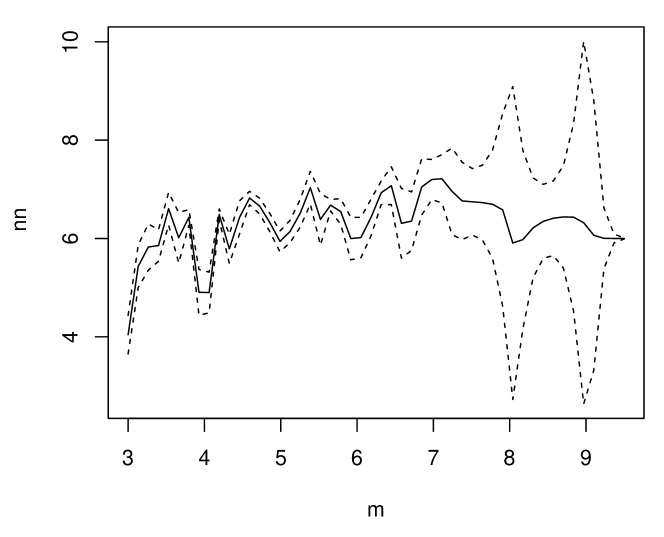
Figure 1. Kernel regression estimate (with 95 between the mean district magnitude and the number of registered parties in Polish county elections.

We begin with setting up the notation to be used throughout the remainder of this article.

Notation 3.

Let:

• $x_{i}^{\downarrow}$ denote the $i$-th largest element of a totally ordered countable set $\{x_{1},x_{2},\ldots\}$,

• $s\in\mathbb{N}_{+}$ be the assembly size, i.e., total number of seats,

• $c\in\mathbb{N}_{+}$ be the number of districts,

• $N\in\mathbb{N}_{+}$ be the number of registered parties,

• $n\in\left\{1,\dots,N\right\}$ be the number of relevant parties,

• $m:=s/c$ be the mean district magnitude,

• $\Delta_{n}$ be the $\left(n-1\right)$-dimensional probability simplex,

• $\mathbf{v}:=\left(v_{1},\dots,v_{N}\right)\in\Delta_{n}$ be the nationwide vote share vector,

• $p_{i}:=v_{i}/\sum_{j=1}^{n}v_{j}^{\downarrow}$ be the nationwide vote share of the $i$-th relevant party, $i=1,\dots,n$, renormalized after excluding non-relevant parties,

• $q_{i}^{\downarrow}:=v_{i}^{\downarrow}/\sum_{j=1}^{i}v_{j}^{\downarrow}$ be the nationwide vote share of the $i$-th largest party, $i=1,\dots,N$, renormalized after excluding all smaller parties,

• $v_{i}^{k}$ be the vote share of the $i$-th party in the $k$-th district, $k=1,\dots,c$,

• $p_{i}^{k}$ be the vote share of the $i$-th relevant party in the $k$-th district renormalized after excluding non-relevant parties,

• $M_{k}\in\mathbb{R}_{+}$ be the Jefferson-D’Hondt multiplier in the $k$-th district,

• $R_{i}^{k}:=\left\{p_{i}^{k}M_{k}\right\}$ be the rounding residual of the $i$-th relevant party in the $k$-th district,

• $\tau\in\left(0,1\right)$ be the statutory threshold,

• $\left\langle x_{i}^{k}\right\rangle$ denote the average of $x_{i}^{k}$ over $k=1,\dots,c$.

2. Theoretical Model

2.1. The “Pot and Ladle” Model of the Jefferson-D’Hondt System

The starting point of our reasoning consists of the “pot and ladle” model of the Jefferson-D’Hondt system, introduced in (Flis et al.,, 2019) and further elaborated (Flis et al.,, 2018), which provides the following closed-form formula for estimating seat counts from nationwide vote shares:

Theorem 4.

Assume there are $n$ relevant parties. If

1. there exists a selection of multipliers $M_{1},\dots,M_{k}$ such that for each $j=1,\dots,n$

   1. rounding residuals average to $1/2$ over districts, i.e., $\left\langle R_{j}^{k}\left(M_{k}\right)\right\rangle=\frac{1}{2}$;

   2. multipliers are not correlated with normalized vote shares, i.e.,$\mathop{\mathrm{C}ov}\left(p_{j}^{k},M_{k}\right)=0$;

2. no seats have been obtained by non-relevant parties;

3. for each $j=1,\dots,n$ the normalized nationwide vote share equals average normalized district-level vote share, i.e., $p_{j}=\left\langle p_{j}^{k}\right\rangle$,

then for each relevant party, $j=1,\dots,n$, the nationwide number of seats is given by

$$s_{j}=p_{j}s+p_{j}\frac{cn}{2}-\frac{c}{2}.$$ (2)

For proof of the above, see (Flis et al.,, 2018). Of the above assumptions, A2 and A3 are essentially political in nature, requiring that there be no anomalies in the spatial distribution of party support (such as regionalisms, malapportionment, or large differences in district magnitudes) that cause district-level electoral results to diverge from nationwide data. In constrast, A1 is rather technical, but can be justified mathematically: under some general distributional assumptions, it can be shown that there exist multipliers for which both A1a and A1b hold approximately, and thus the expected number of seats $\mathop{\mathrm{E}}\left(s_{j}\right)$ is well approximated by (2). Empirical research shows that both sets of assumptions correspond closely to reality, making the “pot-and-ladle” model quite accurate.

One of the advantages of the “pot and ladle” model from our point of view consists of the fact that it includes a mathematically convenient criterion of relevance:

Corollary 5.

Assuming there are no statutory thresholds, the $j$-th party is relevant in the sense of Theorem 4 if and only if

$$p_{j}\geq t:=\frac{1}{2m+n}.$$ (3)

In the above formula, $t$ denotes the natural threshold. The underlying reasoning is quite simple: for $p_{j}<t$, assumptions A1 and A3 lead to a contradiction. But an apparent circularity in reasoning can be noted: the natural threshold $t$ depends on the number of relevant parties, which in turn depends on $n$. This circularity can be eliminated when one recognizes that the above Corollary is equivalent to:

Corollary 6.

Assuming there are no statutory thresholds, the $k$-th largest party is relevant in the sense of Theorem 4 if and only if

$$p_{k}^{\downarrow}\geq t_{k}:=\frac{1}{2m+k}.$$ (4)

In systems employing statutory thresholds as well, there is of course a concurrent criterion that

$$v_{k}^{\downarrow}\geq\tau.$$ (5)

It further follows that:

Corollary 7.

The number of relevant parties appearing in (2) is given by

$$n:=\max\left\{k=1,\dots,N:p_{k}^{\downarrow}\geq\frac{1}{2m+k}~{}\text{and}~{}v_{k}^{\downarrow}\geq\tau\right\}.$$ (6)

2.2. Modeling the Distribution of Party Vote Shares

What is the probability that the $k$-th largest party is relevant under Eq. (4) and under Eq. (5)? It is clear that the answer depends on the distribution of votes among parties (note that unlike in the preceding chapter, the random variable here is the nationwide rather than district-level vector of vote shares). The problem of modeling such distribution is equivalent to a special case of the problem of modeling preference orderings, which is well known in the social choice theory (see, e.g., Regenwetter et al.,, 2006 and Tideman & Plassmann,, 2012). Of those, motivated by the principle of insufficient reason, we choose the Impartial Anonymous Culture (IAC) model which treats each preference profile (and, thus, each distribution of votes among parties) as equiprobable Gehrlein & Fishburn,, 1976; Kuga & Nagatani,, 1974. Accordingly, the vote share vector $\mathbf{v}$ follows the uniform distribution on a discrete grid of points within $\Delta_{N}$, which, as the number of voters approaches infinity, weakly converges to the uniform distribution on $\Delta_{N}$. To simplify calculations, we focus on the limiting case.

Under those distributional assumptions, we arrive at two results regarding the distribution of absolute and normalized vote shares of the $k$-th largest party:

Theorem 8.

If $\mathbf{V\sim}\mathop{\mathrm{U}nif}\left(\Delta_{N}\right)$, where $\mathop{\mathrm{U}nif}\left(\Delta_{N}\right)$ is the uniform distribution on $\Delta_{N}$, then $V_{k}^{\downarrow}$, $k=1,\dots,N$, is distributed according to a continuous distribution supported on $[0,1/k]$ for $k>1$ and on $[1/N,1]$ for $k=1$, with density $f_{V_{k}^{\downarrow}}$ given by:

$$f_{V_{k}^{\downarrow}}\left(x\right):=N\left(N-1\right)\dbinom{N-1}{k-1}\sum\limits_{a=k}^{\min\left(N,\left\lfloor 1/x\right\rfloor\right)}\left(-1\right)^{a-k}\dbinom{N-k}{a-k}\left(1-ax\right)^{N-2}.$$ (7)

Figure 2. Density of the distribution of the voting weight of the $k$-th largest of $4$ players.

Theorem 9.

If $\mathbf{V\sim}\mathop{\mathrm{U}nif}\left(\Delta_{N}\right)$, where $\mathop{\mathrm{U}nif}\left(\Delta_{N}\right)$ is the uniform distribution on $\Delta_{N}$, then $P_{1}^{\downarrow}=1$ with probability $1$, and $P_{k}^{\downarrow}$, $k=2,\dots,N$, is distributed according to a continuous distribution supported on $[0,1/k]$, with density $f_{P_{k}^{\downarrow}}$ given by:

$$f_{P_{k}^{\downarrow}}\left(x\right):=\mathbf{1}_{\left\{z<1/k\right\}}\,k\left(k-1\right)\dbinom{N}{k}\left(1-xk\right)^{k-2}\times\\ \times\sum_{a=k}^{N}\left(-1\right)^{a-k}\dbinom{N-k}{a-k}\left(1+\left(a-k\right)x\right)^{-k}.$$ (8)

For proofs of the above theorems, see Appendix A.

Note that Theorem 8 corresponds to a known earlier result on the order statistics of uniform spacings (Darling,, 1953; Rao & Sobel,, 1980; Devroye,, 1981). However, it is impossible to obtain Theorem 9 from that result alone, and proof techniques employed in the context of uniform spacings are not easily extended to that question. In contrast, our (original) proof of Theorem 8, given in the Appendix A, provides a foundation of the proof of Theorem 9 as well.

2.3. Probability of Relevance

From Theorems 9 and 9 we can obtain a closed-form formula for the probability of the $k$-th largest party being relevant. Recall from (4) that in the absence of a statutory threshold, the $k$-th largest party is relevant if and only if

$$p_{k}^{\downarrow}\geq t_{k}:=\left(2m+k\right)^{-1}.$$ (9)

Thus, we are interested in $\Pr\left(P_{k}^{\downarrow}>t_{k}\right)$. By integrating the density of $P_{k}^{\downarrow}$, we obtain (see Appendix B for details):

$$\Pr\left(P_{k}^{\downarrow}>t_{k}\right)=k\dbinom{N}{k}\sum_{a=k}^{N}\left(-1\right)^{a-k}\dbinom{N-k}{a-k}\frac{1}{a}\left(\frac{2m}{a+2m}\right)^{k-1}.$$ (10)

Likewise, the $k$-th largest party is relevant under a statutory threshold if $v_{k}^{\downarrow}\geq\tau.$By integrating the density of $V_{k}^{\downarrow}$, we obtain:

$$\Pr\left(V_{k}^{\downarrow}>\tau\right)=N\dbinom{N-1}{k-1}\sum_{a=k}^{\min\left(N,\left\lfloor\tau^{-1}\right\rfloor\right)}\left(-1\right)^{a-k}\dbinom{N-k}{a-k}\frac{1}{a}\left(1-a\tau\right)^{N-1}.$$ (11)

2.4. Expected Number of Relevant Parties

Expected number of relevant parties is easy to obtain from the above results. First, let us note that the probability that the $k$-th party is last relevant party can be expressed as the difference of the probabilities of relevance of the $k$-th and $\left(k+1\right)$-th parties (with $\Pr\left(P_{N+1}^{\downarrow}>t_{N+1}\right)=\Pr\left(V_{N+1}^{\downarrow}>\tau\right)=0$):

$$\Pr\left(n=k\right)=\Pr\left(P_{k}^{\downarrow}>t_{k}\right)-\Pr\left(P_{k+1}^{\downarrow}>t_{k+1}\right).$$ (12)

Now from the formula for the expectation of a discrete distribution we have (see Appendix C for details):

$$\mathop{\mathrm{E}}n=\sum_{k=1}^{N}k\Pr\left(n=k\right)=\sum_{k=1}^{N}\Pr\left(P_{k}^{\downarrow}>t_{k}\right)\text{,}$$ (13)

and if statutory thresholds are accounted for,

$$\mathop{\mathrm{E}}n=\min\left\{\sum_{k=1}^{N}\Pr\left(P_{k}^{\downarrow}>t_{k}\right),\sum_{k=1}^{N}\Pr\left(V_{k}^{\downarrow}>\tau\right)\right\}.$$ (14)

We can likewise obtain the formula for the second moment of $n$,

$$\mathop{\mathrm{E}}\left(n^{2}\right)=\sum_{k=1}^{N}k^{2}\Pr\left(n=k\right)=2\sum_{k=2}^{N}k\Pr\left(P_{k}^{\downarrow}>t_{k}\right)-\sum_{k=1}^{N}\Pr\left(P_{k}^{\downarrow}>t_{k}\right)\text{,}$$ (15)

and thus for variance,

$$\mathop{\mathrm{V}ar}\left(n\right)=\mathop{\mathrm{E}}\left(n^{2}\right)-\left(\mathop{\mathrm{E}}n\right)^{2}=$$

$$=2\sum_{k=2}^{N}k\Pr\left(P_{k}^{\downarrow}>t_{k}\right)-\sum_{k=1}^{N}\Pr\left(P_{k}^{\downarrow}>t_{k}\right)-\left(\sum_{k=1}^{N}\Pr\left(P_{k}^{\downarrow}>t_{k}\right)\right)^{2}.$$ (16)

2.5. Plots

The behavior of formulae (10) and (13) is illustrated by the following plots.

Figure 3. Probability of relevance of the $k$-th party, $k=1,\dots,N$, out of $N=12$ (left) or $N=20$ (right) assuming mean district magnitude $m=8$.

Figure 4. Probability of relevance of the $4$-th party out of $N=4,\dots,20$, assuming mean district magnitude $m=8$.

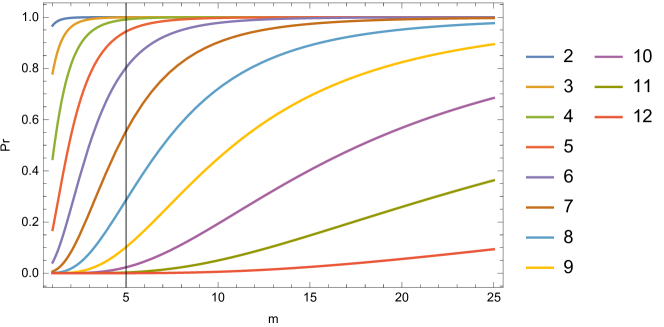
Figure 5. Probability of relevance of the $k$-th party out of $N=12$ as a function of mean district magnitude $m$.

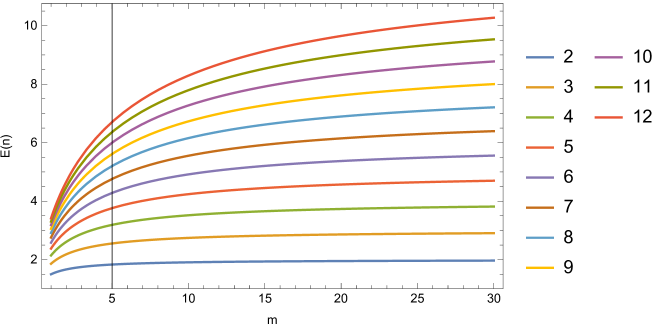
Figure 6. Expected number of relevant parties as a function of mean district magnitude $m$ and the number of registered parties $N=2,\dots,12$.

3. Empirical Test

We have tested our model using two sets of data: general elections results from nine EU countries using the Jefferson–D’Hondt method (with Belgium split into the Flemish and Waloon regions due to the disjointness of their party systems) and Polish county council elections. The European general election dataset is rather small (87 elections), but highly heterogenous in terms of both parameters of interest (i.e., the district magnitude varies between $6.731$ and $150$, and the number of registered parties varies between $3$ and $28$). The Polish county election dataset is more numerous (1564 elections), but more homogenous ($m$ varies between $3$ and $9.5$, and $N$ – between $2$ and $15$).

3.1. General Elections in Nine EU Countries Using Jefferson-D’Hondt

There are currently nine EU member states using the Jefferson–D’Hondt method for parliamentary seat allocation in multimember districts (we exclude countries such as Austria that only use JDH in combination with other methods, e.g., in multi-tiered elections): Belgium, Croatia, the Czech Republic, Finland, Luxembourg, Netherlands, Poland, Portugal, and Spain. For each of those nine countries, we analyze all post-1945 elections held under JDH rule (as noted above, we treat the Belgian general election of 2014, the only one held under pure JDH, as a special case, i.e., as two concurrent but distinct elections in Flemish and Walloon regions). For each election, we have identified the mean district magnitude $m$ and the number of registered national parties (defining a registered national party as a party or a single-list coalition fielding candidates in at least 90% of electoral districts), computed the expected number of relevant parties using our probabilistic model, and compared the outcome with the one arising under the Seat-Product Model. Table 1 gives mean $L_{1}$ errors (absolute deviations from the mean) for our model, the Seat-Product Model, and “naive” $n=N$ model.

country	probabilistic	SPM	$n=N$
Belgium – F	0.128	0.039	0.333
Belgium – W	0.051	0.276	0.428
Croatia	0.226	0.238	1.988
Czech Republic	0.368	0.397	2.002
Finland	0.125	0.235	0.530
Luxembourg	0.112	0.163	0.146
Netherlands	0.750	0.240	1.014
Poland	0.083	0.433	0.792
Portugal	0.433	0.495	1.096
Spain	0.328	0.378	0.848

Table 1. Normalized Mean Absolute Deviation $\left\langle|\operatorname*{\mathbb{E}}n-n|/n\right\rangle$.

As can be seen from the above results, the probabilistic model of the number of relevant parties is an improvement over earlier models like the Seat–Product Model, scoring better for eight of ten tested countries, and worse only for Wallonia (where the whole sample consists of a single election) and Netherlands (where the ease of registering small parties makes the uniform distribution assumption probably unrealistic).

3.2. Polish County Elections

There are currently 314 counties in Poland. In each county, there is a council (varying between 15 and 60 seats) elected using the Jefferson-D’Hondt with the statutory threshold of 5%. Each county is divided into three or more districts with magnitude greater than or equal to $3$. For each county, we analyze all elections between 1998 and 2014 (yielding 1564 elections), again computing the expected number of relevant parties using our probabilistic model and comparing the outcome with the one arising under the Seat-Product Model. Mean error values are given in Table 2.

	mean abs. dev.	mean square error
model	$\left\langle\left|\mathop{\mathrm{E}}n-n\right|\right\rangle$	$\sqrt{\left\langle\left(\mathop{\mathrm{E}}n-n\right)^{2}\right\rangle}$
probabilistic	0.945	1.149
Seat-Product Model	2.068	2.460
$n=N$	2.111	2.466

Table 2. Overall Errors of the Three Alternative Models of the Number of Relevant Parties.

Figure 7. Kernel density estimates of the normalized absolute deviation $|\operatorname*{\mathbb{E}}n-n|/n$ for the probabilistic model (black curve), the Seat-Product Model (blue curve) and the “naive” ($n=N$) model (red curve).

Again, the probabilistic model represents a significant improvement over the alternatives.

Appendix A Distribution of $P_{k}^{\downarrow}$ and $V_{k}^{\downarrow}$

Let $X_{1},\dots,X_{N}$ be independent random variables distributed according to $\mathop{\mathrm{E}xp}\left(1\right)$, i.e., with density $f\left(x\right):=e^{-x}$. It is well known (see, e.g, Jambunathan,, 1954) that

$$\left(\frac{X_{1}}{\sum_{i=1}^{N}X_{i}},\dots,\frac{X_{N}}{\sum_{i=1}^{N}X_{i}}\right)\sim\mathop{\mathrm{U}nif}\left(\Delta_{N}\right).$$ (17)

A.1. $k$-th order statistic $X_{k}^{\downarrow}$

Consider first the density of $X_{k}^{\downarrow}$. We start with the following result by Rényi, (1953):

$$X_{k}^{\downarrow}\overset{d}{=}\sum_{j=k}^{N}\frac{Z_{j}}{j},$$ (18)

where $Z_{j},\dots,Z_{N}\sim\mathop{\mathrm{E}xp}\left(1\right)$ and are i.i.d. Thus,

$$\varphi_{X_{k}^{\downarrow}}(s)=\prod\limits_{j=k}^{N}\left(1-\frac{is}{j}\right)^{-1}=\prod\limits_{j=k}^{N}\frac{j}{j-is}=\frac{\left(k\right)_{N-k+1}}{\left(k-is\right)_{N-k+1}},$$ (19)

wherefore (by Lévy’s inversion formula, Billingsley,, 1995, p. 347, (26.20))

$$f_{X_{k}^{\downarrow}}(x)=\frac{\left(k\right)_{N-k+1}}{2\pi}\int_{-\infty}^{+\infty}\frac{e^{-isx}}{\left(k-is\right)_{N-k+1}}ds.$$ (20)

Let us denote the function under the integral as $\lambda\left(s\right)$. Note that it has $N-k+1$ simple poles at $-ik,\dots,-iN$.

Let us consider a contour $C_{r}:=\left[r,-r\right]\cup A_{r}$, where

$$A_{r}:=\left\{x\in\mathbb{C}:\left(\left|x\right|=r\right)\text{ and }\arg(x)\in(\pi,2\pi)\right\}$$ (21)

is a positively oriented arc from $-r$ to $r$ centered at $0$, and $r>N$. Then by the residue theorem,

$$\oint\nolimits_{C_{r}}\lambda\left(s\right)\,ds=2\pi i\,\sum\nolimits_{j=k}^{N}\mathop{\mathrm{R}es}\left(\lambda,-ij\right).$$ (22)

Let us first consider the integral of $\lambda\left(s\right)$ over $A_{r}$. Let us substitute $s=re^{i\theta}$, where $\theta\in\left(\pi,2\pi\right)$. Then for $s\in A_{r}$ we have

$$\left|\lambda\left(s\right)\right| \leq e^{rx\sin\theta}\prod\limits_{j=k}^{N}\left|\left(j+r\sin\theta-ir\cos\theta\right)^{-1}\right|=$$ (23)

$$= e^{rx\sin\theta}\prod\limits_{j=k}^{N}\left(j^{2}+r^{2}+2jr\sin\theta\right)^{-1},$$ (24)

which is dominated by $e^{rx\sin\theta}r^{-2(N-k+1)}$ as $r\rightarrow\infty$. Therefore by the estimation lemma (Howie,, 2003, Theorem 5.24),

$$\oint\nolimits_{A_{r}}\lambda\left(s\right)\,ds=O\left(e^{rx\sin\theta}r^{-2(N-k+1)}r\right)=O\left(0\right)$$ (25)

as $r\rightarrow\infty$, wherefore

$$\int_{-\infty}^{+\infty}\lambda\left(s\right)\,ds=-2\pi i\,\sum\nolimits_{j=k}^{N}\mathop{\mathrm{R}es}\left(\lambda,-ij\right)$$ (26)

(the minus sign in the integral arises because the contour integral is computed in the reverse direction). Computing the residues, we get

$$\mathop{\mathrm{R}es}\left(\lambda,-ij\right) = \underset{s\rightarrow-ij}{\lim}\left(s+ij\right)e^{-isx}\prod\nolimits_{l=k}^{N}\frac{1}{l-is}=$$ (27)

$$= ie^{-jx}\prod\nolimits_{l=k}^{j-1}\frac{1}{l-j}\prod\nolimits_{l=j+1}^{N}\frac{1}{l-j}=$$ (28)

$$= i\left(-1\right)^{k-j}\frac{1}{\left(j-k\right)!}\frac{1}{\left(N-j\right)!}e^{-jx},$$ (29)

and thus

$$\int_{-\infty}^{+\infty}\lambda\left(s\right)\,ds=-2\pi i\,\sum\nolimits_{j=k}^{N}i\left(-1\right)^{k-j}\frac{1}{\left(j-k\right)!}\frac{1}{\left(N-j\right)!}e^{-jx}=$$ (30)

$$=2\pi\frac{e^{-kx}\left(1-e^{-x}\right)^{N-k}}{\left(N-k\right)!}.$$ (31)

Substituting the above into (19), we obtain the density of $X_{k}^{\downarrow}$:

$$f_{X_{k}^{\downarrow}}(x)=\frac{N!}{\left(k-1\right)!}\frac{e^{-kx}\left(1-e^{-x}\right)^{N-k}}{\left(N-k\right)!}=k\dbinom{N}{k}e^{-kx}\left(1-e^{-x}\right)^{N-k}.$$ (32)

A.2. Vote shares

Let us fix the $k$-th largest order statistic, $X_{k}^{\downarrow}$, at $y$, and let:

• $\Psi^{\downarrow}:=\sum\nolimits_{j=k+1}^{N}X_{j}^{\downarrow},$

• $\Psi^{\uparrow}:=\sum\nolimits_{j=1}^{k-1}X_{j}^{\downarrow},$

• $\Psi:=\sum\nolimits_{j=1}^{N}X_{j}^{\downarrow}=\Psi^{\downarrow}+\Psi^{\uparrow}+X_{k}^{\downarrow}.$

The non-normalized vote share of the $k$-th party is given by

$$V_{k}^{\downarrow}=\frac{X_{k}^{\downarrow}}{\Psi}.$$ (33)

The normalized vote share of the $k$-th party assuming $k$ relevant parties is given by

$$P_{k}^{\downarrow}=\frac{V_{k}^{\downarrow}}{\sum_{j=1}^{k}V_{j}^{\downarrow}}=\frac{V_{k}^{\downarrow}}{\Psi}\frac{\Psi}{\sum_{j=1}^{k}V_{k}^{\downarrow}}=\frac{V_{k}^{\downarrow}}{V_{k}^{\downarrow}+\Psi^{\uparrow}}.$$ (34)

Note that $\Psi^{\uparrow}=\sum\nolimits_{j=1}^{k-1}Y_{j}$, where $Y_{j}\sim\mathop{\mathrm{E}xp}\left(1\right)$ truncated to $(y,\infty)$, and $\Psi^{\downarrow}=\sum\nolimits_{j=1}^{N-k}Z_{j}$, where $Z_{j}\sim\mathop{\mathrm{E}xp}\left(1\right)$ truncated to $(0,y)$. Then the density of $Z_{j}$ is given by

$$f_{Z}(x)=\frac{e^{-x}}{F(y)-F(0)}=\frac{e^{-x}}{1-e^{-y}}$$ (35)

for $x\in(0,y)$, and the density of $Y_{j}$ is given by

$$f_{Y}(x)=\frac{e^{-x}}{1-F(y)}=e^{y-x}$$ (36)

for $x\in(y,\infty)$, and their characteristic functions are given by, respectively,

$$\varphi_{Z}\left(t\right)=\frac{1}{1-e^{-y}}\int_{0}^{y}e^{itx-x}dx=\frac{i}{i+t}\frac{e^{y}-e^{ity}}{e^{y}-1},$$ (37)

and

$$\varphi_{Y}\left(t\right)=e^{y}\int_{y}^{\infty}e^{itx-x}dx=\frac{i}{i+t}e^{ity}.$$ (38)

Hence, the conditional characteristic function of $\Psi^{\downarrow}$ is given by

$$\varphi_{\Psi^{\downarrow}|X_{k}^{\downarrow}}(t,y)=\left(\frac{i}{i+t}\frac{e^{y}-e^{ity}}{e^{y}-1}\right)^{N-k}=\left(1-it\right)^{k-N}\left(\frac{e^{y}-e^{ity}}{e^{y}-1}\right)^{N-k},$$ (39)

the conditional characteristic function of $\Psi^{\uparrow}$ by

$$\varphi_{\Psi^{\uparrow}|X_{k}^{\downarrow}}(t,y)=\left(\frac{i}{i+t}e^{ity}\right)^{k-1}=\left(1-it\right)^{1-k}e^{ity\left(k-1\right)},$$ (40)

and the conditional characteristic function of $\Psi$ by

$$\varphi_{\Psi|X_{k}^{\downarrow}}(t,y) = e^{ity}\left(1-it\right)^{1-N}\left(\frac{e^{y}-e^{ity}}{e^{y}-1}\right)^{N-k}e^{ity\left(k-1\right)}=$$ (41)

$$= \left(1-it\right)^{1-N}\left(\frac{e^{y}-e^{ity}}{e^{y}-1}\right)^{N-k}e^{ityk}.$$ (42)

By the binomial theorem,

$$\left(e^{y}-e^{ity}\right)^{N-k}=\sum\nolimits_{a=0}^{N-k}\dbinom{N-k}{a}e^{y(N-k-a)}e^{i(ty+\pi)a},$$ (43)

wherefore

$$\varphi_{\Psi^{\downarrow}|X_{k}^{\downarrow}}(t,y)=(e^{y}-1)^{k-N}\sum\nolimits_{a=0}^{N-k}\dbinom{N-k}{a}\left(1-it\right)^{k-N}e^{y(N-k-a)}e^{i\pi a}e^{itya}.$$ (44)

Again by Levy’s inversion formula,

$$f_{\Psi^{\downarrow}|X_{k}^{\downarrow}}(x,y)=\frac{1}{2\pi}(e^{y}-1)^{k-N}\int_{-\infty}^{+\infty}\sum\nolimits_{a=0}^{N-k}\dbinom{N-k}{a}\left(1-it\right)^{k-N}e^{y(N-k-a)}e^{i\pi a}e^{itya-itx}\,dt=$$ (45)

$$=\frac{1}{2\pi}(e^{y}-1)^{k-N}\sum\nolimits_{a=0}^{N-k}\dbinom{N-k}{a}e^{y(N-k-a)}i^{2a}\int_{-\infty}^{+\infty}\left(1-it\right)^{k-N}e^{it(ya-x)}\,dt=$$ (46)

$$=\frac{1}{2\pi}(e^{y}-1)^{k-N}\sum\nolimits_{a=0}^{N-k}\left(-1\right)^{a}\dbinom{N-k}{a}e^{y(N-k-a)}\tciFourier\left\{\left(1-it\right)^{k-N}\right\}(x-ya)=$$ (47)

$$=\frac{1}{2\pi}(e^{y}-1)^{k-N}\sum\nolimits_{a=k}^{N}\left(-1\right)^{a-k}\dbinom{N-k}{a-k}e^{y(N-a)}\tciFourier\left\{\left(1-it\right)^{-(N-k)}\right\}(x-y(a-k)).$$ (48)

Now by Bateman,, 1954, § 3.2 (3), p. 118,

$$f_{\Psi^{\downarrow}|X_{k}^{\downarrow}}(x,y)=$$ (49)

$$=\frac{(e^{y}-1)^{k-N}}{2\pi}\sum_{a=k}^{N}\left(-1\right)^{a-k}\dbinom{N-k}{a-k}e^{y(N-a)}\left\{\begin{array}[]{cc}\frac{2\pi\left(x-y(a-k)\right)^{N-k-1}e^{-(x-y(a-k))}}{\Gamma\left(N-k\right)}&:x>y(a-k)\\ 0&:x\leq y(a-k)\end{array}\right.=$$ (52)

$$=\frac{(1-e^{-y})^{k-N}}{\left(N-k-1\right)!}e^{-x}\sum\nolimits_{a=k}^{\min\left(N,\left\lfloor x/y\right\rfloor+k\right)}\left(-1\right)^{a-k}\dbinom{N-k}{a-k}\left(x-y(a-k)\right)^{N-k-1}.$$ (53)

Likewise,

$$f_{\Psi^{\uparrow}|X_{k}^{\downarrow}}(x,y) = \frac{1}{2\pi}\int_{-\infty}^{+\infty}\left(1-it\right)^{1-k}e^{ity(k-1)-itx}\,dt=$$ (54)

$$= \frac{1}{2\pi}\mathcal{\tciFourier}\left\{\left(1-it\right)^{1-k}\right\}(x-y(k-1))=$$ (55)

$$= \frac{1}{\left(k-2\right)!}\left\{\begin{array}[]{cc}\left(x-y(k-1)\right)^{k-2}e^{y(k-1)-x}&:x>y(k-1)\\ 0&:x\leq y(k-1)\end{array}\right.,$$ (58)

and

$$f_{\Psi^{\uparrow}+X_{k}^{\downarrow}|X_{k}^{\downarrow}}(x,y)=f_{\Psi^{\uparrow}|X_{k}^{\downarrow}}(x-y,y)=\frac{1}{\left(k-2\right)!}\left\{\begin{array}[]{cc}\left(x-yk\right)^{k-2}e^{yk-x}&:x>yk\\ 0&:x\leq yk\end{array}\right..$$ (59)

A.3. Joint density and ratio

Joint density is easy to obtain from the above results:

$$f_{\Psi^{\uparrow}+X_{k}^{\downarrow},X_{k}^{\downarrow}}(x,y) = \frac{1}{\left(k-2\right)!}\left\{\begin{array}[]{cc}\left(x-yk\right)^{k-2}e^{yk-x}&:x>yk\\ 0&:x\leq yk\end{array}\right.\times k\dbinom{N}{k}e^{-ky}\left(1-e^{-y}\right)^{N-k}=$$ (62)

$$= \mathbf{1}_{\left\{x>yk\right\}}\frac{k}{\left(k-2\right)!}\dbinom{N}{k}\left(1-e^{-y}\right)^{N-k}\left(x-yk\right)^{k-2}e^{-x}.$$ (63)

And the density of the ratio $P_{k}^{\downarrow}=X_{k}^{\downarrow}/\left(X_{k}^{\downarrow}+\Psi^{\uparrow}\right)$ is given by

$$f_{P_{k}^{\downarrow}}\left(z\right) = \int_{0}^{\infty}x\,\mathbf{1}_{\left\{x>zk\right\}}\frac{k}{\left(k-2\right)!}\dbinom{N}{k}\left(1-e^{-zx}\right)^{N-k}\left(x-zxk\right)^{k-2}e^{-x}\,dx=$$ (64)

$$= \mathbf{1}_{\left\{z<1/k\right\}}\frac{k}{\left(k-2\right)!}\dbinom{N}{k}\left(1-zk\right)^{k-2}\int_{0}^{\infty}x^{k-1}e^{-x}\,\left(1-e^{-zx}\right)^{N-k}\,dx=$$ (65)

$$= \mathbf{1}_{\left\{z<1/k\right\}}\frac{k}{\left(k-2\right)!}\dbinom{N}{k}\left(1-zk\right)^{k-2}\int_{0}^{\infty}x^{k-1}e^{-x}\,\sum_{a=0}^{N-k}\left(-1\right)^{a}\dbinom{N-k}{a}e^{-zxa}\,dx=$$ (66)

$$= \mathbf{1}_{\left\{z<1/k\right\}}\frac{k}{\left(k-2\right)!}\dbinom{N}{k}\left(1-zk\right)^{k-2}\sum_{a=0}^{N-k}\left(-1\right)^{a}\dbinom{N-k}{a}\int_{0}^{\infty}x^{k-1}e^{-zxa-x}\,dx=$$ (67)

$$= \mathbf{1}_{\left\{z<1/k\right\}}\frac{k}{\left(k-2\right)!}\dbinom{N}{k}\left(1-zk\right)^{k-2}\sum_{a=0}^{N-k}\left(-1\right)^{a}\dbinom{N-k}{a}\left(1+az\right)^{-k}\Gamma\left(k\right)=$$ (68)

$$= \mathbf{1}_{\left\{z<1/k\right\}}\,k\left(k-1\right)\dbinom{N}{k}\left(1-zk\right)^{k-2}\sum_{a=0}^{N-k}\left(-1\right)^{a}\dbinom{N-k}{a}\left(1+az\right)^{-k}.$$ (69)

Appendix B Obtaining the probability of relevance

We are interested in $\Pr\left(P_{k}^{\downarrow}>t_{k}\right)$. By integrating the density of $P_{k}^{\downarrow}$, we obtain

$$\Pr\left(P_{k}^{\downarrow}>t_{k}\right)=\int_{\left(2m+k\right)^{-1}}^{k^{-1}}f_{P_{k}^{\downarrow}}\left(x\right)\,dx=$$ (70)

$$=k\left(k-1\right)\dbinom{N}{k}\sum_{a=0}^{N-k}\left(-1\right)^{a}\dbinom{N-k}{a}\int_{\left(2m+k\right)^{-1}}^{k^{-1}}\frac{\left(1-xk\right)^{k-2}}{\left(1+ax\right)^{k}}\,dx=$$ (71)

$$=k\left(k-1\right)\dbinom{N}{k}\sum_{a=0}^{N-k}\left(-1\right)^{a}\dbinom{N-k}{a}\left.\frac{-1}{\left(k-1\right)\left(a+k\right)}\left(\frac{1-xk}{1+ax}\right)^{k-1}\right|_{x=\left(2m+k\right)^{-1}}^{x=k^{-1}}=$$ (72)

$$=k\left(k-1\right)\dbinom{N}{k}\sum_{a=0}^{N-k}\left(-1\right)^{a}\dbinom{N-k}{a}\frac{1}{\left(k-1\right)\left(a+k\right)}\left(\frac{2m}{a+k+2m}\right)^{k-1}=$$ (73)

$$=k\dbinom{N}{k}\sum_{a=k}^{N}\left(-1\right)^{a-k}\dbinom{N-k}{a-k}\frac{1}{a}\left(\frac{2m}{a+2m}\right)^{k-1}.$$ (74)

Likewise, we are interested in $\Pr\left(V_{k}^{\downarrow}>\tau\right)$. By integrating the density of $V_{k}^{\downarrow}$, we obtain

$$\Pr\left(V_{k}^{\downarrow}>\tau\right)=\int_{\tau}^{k^{-1}}f_{V_{k}^{\downarrow}}\left(x\right)\,dx=$$ (75)

$$=N\left(N-1\right)\dbinom{N-1}{k-1}\int_{\tau}^{k^{-1}}\sum\limits_{a=k}^{\min\left(N,\left\lfloor 1/x\right\rfloor\right)}\left(-1\right)^{a-k}\dbinom{N-k}{a-k}\left(1-ax\right)^{N-2}\,dx=$$ (76)

$$=N\left(N-1\right)\dbinom{N-1}{k-1}\sum_{a=k}^{\min\left(N,\left\lfloor\tau^{-1}\right\rfloor\right)}\left(-1\right)^{a-k}\dbinom{N-k}{a-k}\int_{\tau}^{a^{-1}}\left(1-ax\right)^{N-2}\,dx=$$ (77)

$$=N\left(N-1\right)\dbinom{N-1}{k-1}\sum_{a=k}^{\min\left(N,\left\lfloor\tau^{-1}\right\rfloor\right)}\left(-1\right)^{a-k}\dbinom{N-k}{a-k}\frac{\left(1-a\tau\right)^{N-1}}{a\left(N-1\right)}=$$ (78)

$$=N\dbinom{N-1}{k-1}\sum_{a=k}^{\min\left(N,\left\lfloor\tau^{-1}\right\rfloor\right)}\left(-1\right)^{a-k}\dbinom{N-k}{a-k}\frac{1}{a}\left(1-a\tau\right)^{N-1}.$$ (79)

Appendix C Obtaining the moments of the distribution of the number of relevant parties

First moment (expectation):

$$\mathop{\mathrm{E}}n=\sum_{k=1}^{N}k\Pr\left(n=k\right)=\sum_{k=1}^{N}k\Pr\left(P_{k}^{\downarrow}>t_{k}\right)-\sum_{k=1}^{N-1}k\Pr\left(P_{k+1}^{\downarrow}>t_{k+1}\right)=$$ (80)

$$=\sum_{k=1}^{N}k\Pr\left(P_{k}^{\downarrow}>t_{k}\right)-\sum_{k=2}^{N}\left(k-1\right)\Pr\left(P_{k}^{\downarrow}>t_{k}\right)=$$ (81)

$$=\sum_{k=1}^{N}k\Pr\left(P_{k}^{\downarrow}>t_{k}\right)-\sum_{k=2}^{N}k\Pr\left(P_{k}^{\downarrow}>t_{k}\right)+\sum_{k=2}^{N}\Pr\left(P_{k}^{\downarrow}>t_{k}\right)=\sum_{k=1}^{N}\Pr\left(P_{k}^{\downarrow}>t_{k}\right).$$ (82)

Second moment:

$$\mathop{\mathrm{E}}\left(n^{2}\right)=\sum_{k=1}^{N}k^{2}\Pr\left(n=k\right)=\sum_{k=1}^{N}k^{2}\Pr\left(P_{k}^{\downarrow}>t_{k}\right)-\sum_{k=1}^{N-1}k^{2}\Pr\left(P_{k+1}^{\downarrow}>t_{k+1}\right)=$$ (83)

$$=\sum_{k=1}^{N}k^{2}\Pr\left(P_{k}^{\downarrow}>t_{k}\right)-\sum_{k=2}^{N}\left(k-1\right)^{2}\Pr\left(P_{k}^{\downarrow}>t_{k}\right)=$$ (84)

$$=\Pr\left(P_{1}^{\downarrow}>t_{1}\right)-\sum_{k=2}^{N}\Pr\left(P_{k}^{\downarrow}>t_{k}\right)+2\sum_{k=2}^{N}k\Pr\left(P_{k}^{\downarrow}>t_{k}\right)=$$ (85)

$$=2\sum_{k=2}^{N}k\Pr\left(P_{k}^{\downarrow}>t_{k}\right)-\sum_{k=1}^{N}\Pr\left(P_{k}^{\downarrow}>t_{k}\right).$$ (86)

References

- Barceló & Muraoka, (2018) Barceló, Joan, & Muraoka, Taishi. 2018. The Effect of Variance in District Magnitude on Party System Inflation. Electoral Studies, 54(Aug.), 44–55.
- Bateman, (1954) Bateman, Harry. 1954. Tables of Integral Transforms. New York, NY: McGraw-Hill.
- Billingsley, (1995) Billingsley, Patrick. 1995. Probability and Measure. Third ed. edn. Wiley Series in Probability and Statistics. Hoboken, N.J: Wiley.
- Boratyn et al., (2019) Boratyn, Daria, Kirsch, Werner, Słomczyński, Wojciech, Stolicki, Dariusz, & Życzkowski, Karol. 2019 (May). Average Weights and Power in Weighted Voting Games. Tech. rept. arXiv: 1905.04261 [cs.GT].
- Colomer, (2004) Colomer, Josep M. 2004. The Handbook of Electoral System Choice. London: Palgrave Macmillan.
- Cox, (1997) Cox, Gary W. 1997. Making Votes Count: Strategic Coordination in the World’s Electoral Systems. Political Economy of Institutions and Decisions. Cambridge, UK: Cambridge University Press.
- Darling, (1953) Darling, Donald A. 1953. On a Class of Problems Related to the Random Division of an Interval. The Annals of Mathematical Statistics, 24(2), 239–253.
- Devroye, (1981) Devroye, Luc. 1981. Laws of the Iterated Logarithm for Order Statistics of Uniform Spacings. The Annals of Probability, 9(5), 860–867.
- Duverger, (1951) Duverger, Maurice. 1951. Les Partis Politiques. Paris: Le Seuil.
- Duverger, (1954) Duverger, Maurice. 1954. Political Parties: Their Organization and Activity in the Modern State. London: Methuen & Co.
- Flis et al., (2018) Flis, Jarosław, Słomczyński, Wojciech, & Stolicki, Dariusz. 2018 (May). Pot and Ladle: Seat Allocation and Seat Bias Under the Jefferson-D’Hondt Method. Tech. rept. arXiv: 1805.08291 [physics.soc-ph].
- Flis et al., (2019) Flis, Jarosław, Słomczyński, Wojciech, & Stolicki, Dariusz. 2019. Pot and Ladle: A Formula for Estimating the Distribution of Seats Under the Jefferson–D’hondt Method. Public Choice, July.
- Gehrlein & Fishburn, (1976) Gehrlein, William V., & Fishburn, Peter C. 1976. Condorcet’s Paradox and Anonymous Preference Profiles. Public Choice, 26(1), 1–18.
- Happacher, (2001) Happacher, Max. 2001. The Discrepancy Distribution of Stationary Multiplier Rules for Rounding Probabilities. Metrika, 53(2), 171–181.
- Howie, (2003) Howie, John M. 2003. Complex Analysis. Springer Undergraduate Mathematics Series. London–New York, NY: Springer.
- Jambunathan, (1954) Jambunathan, M. V. 1954. Some Properties of Beta and Gamma Distributions. The Annals of Mathematical Statistics, 25(2), 401–405.
- Janson & Linusson, (2011) Janson, Svante, & Linusson, Svante. 2011 (Apr.). The Probability of the Alabama Paradox. Tech. rept. arXiv: 1104.2137 [math.PR].
- Kuga & Nagatani, (1974) Kuga, Kiyoshi, & Nagatani, Hiroaki. 1974. Voter Antagonism and the Paradox of Voting. Econometrica, 42(6), 1045–1067.
- Laakso, (1979) Laakso, Markku. 1979. The Maximum Distortion and the Problem of the First Divisor of Different P.R. Systems. Scandinavian Political Studies, 2(2), 161–170.
- Li & Shugart, (2016) Li, Yuhui, & Shugart, Matthew S. 2016. The Seat Product Model of the Effective Number of Parties: A Case For Applied Political Science. Electoral Studies, 41(Mar.), 23–34.
- Lijphart, (1990) Lijphart, Arend. 1990. The Political Consequences of Electoral Laws, 1945-85. American Political Science Review, 84(2), 481–496.
- Lijphart & Gibberd, (1977) Lijphart, Arend, & Gibberd, Robert W. 1977. Thresholds and Payoffs in List Systems of Proportional Representation. European Journal of Political Research, 5(3), 219–244.
- Loosemore & Hanby, (1971) Loosemore, John, & Hanby, Victor J. 1971. The Theoretical Limits of Maximum Distortion: Some Analytic Expressions for Electoral Systems. British Journal of Political Science, 1(4), 467–477.
- Palomares & Ramírez González, (2003) Palomares, Antonio, & Ramírez González, Victoriano. 2003. Thresholds of the Divisor Methods. Numerical Algorithms, 34(2-4), 405–415.
- Rae, (1967) Rae, Douglas W. 1967. The Political Consequences of Electoral Laws. New Haven, CT: Yale University Press.
- Rae et al., (1971) Rae, Douglas W., Hanby, Victor J., & Loosemore, John. 1971. Thresholds of Representation and Thresholds of Exclusion. An Analytic Note on Electoral Systems. Comparative Political Studies, 3(4), 479–488.
- Rao & Sobel, (1980) Rao, J. S., & Sobel, Milton. 1980. Incomplete Dirichlet Integrals with Applications to Ordered Uniform Spacings. Journal of Multivariate Analysis, 10(4), 603–610.
- Regenwetter et al., (2006) Regenwetter, Michel, Grofman, Bernard, Tsetlin, Ilia, & Marley, A.A.J. 2006. Behavioral Social Choice: Probabilistic Models, Statistical Inference, and Applications. Cambridge, UK: Cambridge University Press.
- Rényi, (1953) Rényi, Alfréd. 1953. On the Theory of Order Statistics. Acta Mathematica Academiae Scientiarum Hungaricae, 4(3-4), 191–231.
- Rokkan, (1968) Rokkan, Stein. 1968. Elections: Electoral Systems. Pages 6–21 of: Sills, David L. (ed), International Encyclopaedia of the Social Sciences, vol. 5.
- Schuster et al., (2003) Schuster, Karsten, Pukelsheim, Friedrich, Drton, Mathias, & Draper, Norman R. 2003. Seat Biases of Apportionment Methods for Proportional Representation. Electoral Studies, 22(4), 651–676.
- Schwingenschlögl & Drton, (2004) Schwingenschlögl, Udo, & Drton, Mathias. 2004. Seat Allocation Distributions and Seat Biases of Stationary Apportionment Methods for Proportional Representation. Metrika, 60(2), 191–202.
- Shugart & Taagepera, (2017) Shugart, Matthew S., & Taagepera, Rein. 2017. Votes from Seats. Logical Models of Electoral Systems. Cambridge, UK: Cambridge University Press.
- Singer & Gershman, (2018) Singer, Matthew, & Gershman, Zachary. 2018. Do Changes in District Magnitude Affect Electoral Fragmentation? Evidence Over Time at the District Level. Electoral Studies, 54(Aug.), 172–181.
- Taagepera, (1989) Taagepera, Rein. 1989. Empirical Threshold of Representation. Electoral Studies, 8(2), 105–116.
- Taagepera, (1998a) Taagepera, Rein. 1998a. Effective Magnitude and Effective Threshold. Electoral Studies, 17(4), 393–404.
- Taagepera, (1998b) Taagepera, Rein. 1998b. Nationwide Inclusion and Exclusion Thresholds of Representation. Electoral Studies, 17(4), 405–417.
- Taagepera, (2002) Taagepera, Rein. 2002. Nationwide Threshold of Representation. Electoral Studies, 21(3), 383–401.
- Taagepera, (2007) Taagepera, Rein. 2007. Predicting Party Sizes: The Logic of Simple Electoral Systems. Oxford, UK: Oxford University Press.
- Taagepera & Laakso, (1980) Taagepera, Rein, & Laakso, Marku. 1980. Proportionality Profiles of West European Electoral Systems. European Journal of Political Research, 8(4), 423–446.
- Taagepera & Shugart, (1989) Taagepera, Rein, & Shugart, Matthew S. 1989. Seats and Votes: The Effects and Determinants of Electoral Systems. New Haven, CT: Yale University Press.
- Taagepera & Shugart, (1993) Taagepera, Rein, & Shugart, Matthew Soberg. 1993. Predicting the Number of Parties: A Quantitative Model of Duverger’s Mechanical Effect. American Political Science Review, 87(2), 455–464.
- Tideman & Plassmann, (2012) Tideman, T. Nicolaus, & Plassmann, Florenz. 2012. Modeling the Outcomes of Vote-Casting in Actual Elections. Pages 217–251 of: Felsenthal, Dan S., & Machover, Moshé (eds), Electoral Systems. Paradoxes, Assumptions, and Procedures. Berlin–Heidelberg: Springer.
- Ziegfeld, (2013) Ziegfeld, Adam. 2013. Are Higher-Magnitude Electoral Districts Always Better for Small Parties? Electoral Studies, 32(1), 63–77.