Query Optimization Properties of Modified Valuation-Based Systems

Abstract

Valuation-Based System can represent knowledge in different domains including probability theory, Dempster-Shafer theory and possibility theory. More recent studies show that the framework of VBS is also appropriate for representing and solving Bayesian decision problems and optimization problems. In this paper after introducing the valuation based system (VBS) framework, we present Markov-like properties of VBS and a method for resolving queries to VBS.

1 Introduction

Though graphical representation of a domain knowledge has quite long history, its full potential has not been recognized until recently. We should mention here pioneering works of J. Pearl, reported in his monography published in 1988 [?]. Further development in this domain has been achieved by Shenoy and Shafer [?] who adopted a method used in solving nonserial dynamic programming problems [?]. This trick proved to be very fruitful and gave growth to a unified framework for uncertainty representation and reasoning, called Valuation-Based System, VBS for short [?]. It can represent knowledge in different domains including probability theory, Dempster-Shafer theory and possibility theory. More recent studies show that the framework of VBS is also appropriate for representing and solving Bayesian decision problems [?] and optimization problems [?]. The graphical representation is called a valuation network, and the method for solving problems is called the fusion algorithm. Closely related to VBS is the algorithm of Lauritzen and Spiegelhalter [?] and HUGIN approach developed by Jensen and his co-workers [?].

A Bayesian network (as well as its generalization - VBS) can be regarded as a summary of an expert’s experience with an implicit population. Detailed documentation of such knowledge with an explicit population is stored in a database. It appears that there exists a strong connection between these two approaches. First of all, databases are used for knowledge acquisition and Bayesian network identification - see [?] or [?] for a deeper discussion. Studies by Wen [?], and Wong, Xiang and Nie [?] establish a link between knowledge-based systems for probabilistic reasoning and relational databases. Particularly, they show that the belief update in a Bayesian network can be processed as an ordinary query, and the techniques for query optimization are directly applicable to updating beliefs. The same idea we find in Thoma’s [?] works, who proposed a scheme for storing Shafer’s belief functions which generalizes graphical models.

In this paper after introducing the valuation based system framework (Section 2), we present Markov-like properties of VBS (Section 3) and a method for resolving queries to VBS (Section 4).

2 Valuation Based Systems

The VBS framework was introduced in [?]. In VBS, a domain knowledge is represented by entities called variables and valuations. Further, two operations called combination and marginalization are defined on valuations to perform a local computational method for computing marginals of the joint valuation. The basic components of VBS can be characterized as follows.

Valuations

Let $\mbox{{$\cal X$}}=\{x_{1},x_{2},...x_{n}\}$ be a finite set of variables and $\Theta_{i}$ be the domain (called also frame), i.e. a discrete set of possible values of i-th variable. If h is a finite non-empty set of variables then $\Theta(h)$ denotes the Cartesian product of $\Theta_{i}$ for $x_{i}$ in $h$, i.e. $\Theta(h)=\times\{\Theta_{i}|x_{i}\in h\}$. $\cal R$ stands for a set of non-negative reals. For each subset s of $\cal X$ there is a set $D(s)$ called the domain of a valuation. For instance in the case of probabilistic systems $D(s)$ equals to $\Theta(s)$, while under the belief function framework $D(s)$ equals to the power set of $\Theta(s)$, i.e. $D(s)=2^{\Theta(s)}$. Valuations, being primitives in the VBS framework, can be characterized as mappings $\sigma:D(s)\rightarrow\mbox{{$\cal R$}}$. In the sequel valuations will be denoted by lower-case Greek letters, $\rho$, $\sigma$, $\tau$, and so on. Following Shenoy [?] we distinguish three categories of valuations:

• Proper valuations, $\cal P$, represent knowledge that is partially coherent. (Coherent knowledge means knowledge that has well defined semantics.) This notion plays an important role in the theory of belief functions: by proper valuation it is understood an unnormalized commonality function.

• Normal valuations, $\cal N$, represent another kind of partially coherent knowledge. For instance, in probability theory, a normal valuation is a function whose values sum to 1. Particularly, the elements of $\mbox{{$\cal P$}}\cap\mbox{{$\cal N$}}$ are called proper normal valuations; they represent knowledge that is completely coherent or knowledge that has well-defined semantics.

• Positive normal valuations: it is a subset $\mbox{{$\cal U$}}_{s}$ of $\mbox{{$\cal N$}}_{s}$ consisting of all valuations that have unique identities in $\mbox{{$\cal N$}}_{s}$.

Further there are two types of special valuations:

• Zero valuations represent knowledge that is internally inconsistent, i.e. knowledge whose truth value is always false; e.g., in probability theory by zero valuation we understand a valuation that is identically zero. It is assumed that for each $s\subseteq\mbox{{$\cal X$}}$ there is at most one valuation $\zeta_{s}\in\mbox{{$\cal V$}}_{s}$ . The set of all zero valuations is denoted by $\cal Z$.

• Identity valuations, I, represent total ignorance, i.e. lack of knowledge. In probability theory an identity valuation corresponds to the uniform probability distribution. It is assumed that for each $s\subseteq\mbox{{$\cal X$}}$ the commutative semigroup (w.r.t. the binary operation $\otimes$ defined later) $\mbox{{$\cal N$}}_{s}\cup\{\zeta_{s}\}$ has an identity $\iota_{s}\in\mbox{{$\cal V$}}_{s}$ . Commutative semigroup may have at most one identity [?].

Combination

By combination we understand a mapping $\otimes:\mbox{{$\cal V$}}\times\mbox{{$\cal V$}}\rightarrow\mbox{{$\cal N$}}\cup\mbox{{$\cal Z$}}$ that satisfies the following six axioms:

(C1)

If $\rho\in\mbox{{$\cal V$}}_{r}$ and $\sigma\in\mbox{{$\cal V$}}_{s}$ then $\rho\otimes\sigma\in\mbox{{$\cal V$}}_{r\cup s}$;

(C2)

$\rho\otimes(\sigma\otimes\tau)=(\rho\otimes\sigma)\otimes\tau$;

(C3)

$\rho\otimes\sigma=\sigma\otimes\rho$;

(C4)

If $\rho\in\mbox{{$\cal V$}}_{r}$ and zero valuation $\zeta_{s}$ exists then $\rho\otimes\zeta_{s}\in\mbox{{$\cal V$}}_{r\cup s}$.

(C5)

For each $s\subseteq\mbox{{$\cal X$}}$ there exists an identity valuation $\iota_{s}\in\mbox{{$\cal N$}}_{s}\cup\{\zeta_{s}\}$ such that for each valuation $\sigma\in\mbox{{$\cal N$}}_{s}\cup\{\zeta_{s}\}$, $\sigma\otimes\iota_{s}=\sigma$.

(C6)

It is assumed that the set $\mbox{{$\cal N$}}_{\emptyset}$ consists of exactly one element denoted $\iota_{\emptyset}$ .

In practice combination of two valuations is implemented as follows. Let (+) be a binary operation on $\cal R$. Then $(\sigma\otimes\rho)(x)=\sigma(x.s)(+)\rho(x.r)$ where $x$ is an element from $D(s)$ and $x.r$, $x.s$ stand for the projection (relying upon dropping unnecessary variables) of $x$ onto the appropriate domain $D(r)$ or $D(s)$. In probability theory combination corresponds to pointwise multiplication followed by normalization, and in Dempster-Shafer theory to the Dempster rule of combination.

In the field of uncertain reasoning combination corresponds to aggregation of knowledge: when $\rho$ and $\sigma$ represent our knowledge about variables in subsets $r$ and $s$ of $\cal X$ then the valuation $\rho\otimes\sigma$ represents the aggregated knowledge about variables in $r\cup s$. Moreover Wen [?], and Wong, Xiang and Nie [?] showed that under probabilistic context combination corresponds to the (generalized) join operation used in the data-based systems. Hence the belief update in a Bayesian network can be processed as an ordinary query, and the techniques for query optimization are directly applicable to updating beliefs. Similar idea we find in Thoma’s [?] works, who proposed a scheme for storing Shafer’s belief functions.

If $\rho\otimes\sigma$ is a zero valuation, we say that $\rho$ and $\sigma$ are inconsistent. On the other hand, if $\rho\otimes\sigma$ is a normal valuation, then we say that $\rho$ and $\sigma$ are consistent.

It is important to notice, that an implication of axioms C1 - C3 is that the set $\mbox{{$\cal N$}}_{s}\cup\{\zeta_{s}\}$ together with the combination operator is a commutative semigroup [?]. If zero valuation $\zeta_{s}$ exists then $\zeta_{s}$ is - by axiom C4 - the zero of this semigroup. Similarly, by axiom C5, the identity valuation is the identity of the semigroup $\mbox{{$\cal N$}}_{s}\cup\{\zeta_{s}\}$.

Marginalization

While combination results in knowledge expansion, marginalization results in knowledge contraction. Let $s$ be a non-empty subset of $\cal X$. It is assumed that for each variable X in $s$ there is a mapping $\downarrow(s-\{X\}):\mbox{{$\cal V$}}_{s}\rightarrow\mbox{{$\cal V$}}_{s-\{X\}}$, called marginalization to $s-\{X\}$ or deletion of $X$, that satisfies the next six axioms:

(M1)

Suppose $\sigma\in\mbox{{$\cal V$}}_{s}$ and suppose $X,Y\in s$. Then
$(\sigma^{\downarrow(s-\{X\})})^{\downarrow(s-\{X,Y\})}=(\sigma^{\downarrow(s-\{Y\})})^{\downarrow(s-\{X,Y\})}$ ;

(M2)

If zero valuation exists, then $\zeta_{s}^{\downarrow(s-\{X\})}=\zeta_{s-\{X\}}$;

(M3)

$\sigma^{\downarrow(s-{X})}\in\mbox{{$\cal N$}}$ if and only if $\sigma\in\mbox{{$\cal N$}}$ ;

(M4)

If $\sigma\in\mbox{{$\cal U$}}$ then $\sigma^{\downarrow(s-{X})}\in\mbox{{$\cal U$}}$;

(CM1)

Suppose $\rho\in\mbox{{$\cal V$}}_{r}$ and $\sigma\in\mbox{{$\cal V$}}_{s}$. Suppose $X\not\in r$ and $X\in s$. Then

$(\rho\otimes\sigma)^{\downarrow((r\cup s)-\{X\})}=\rho\otimes\sigma^{\downarrow(s-\{X\})}$

(CM2)

Suppose $\sigma\in\mbox{{$\cal N$}}_{s}$. Suppose $r\subseteq s$ and suppose that $\iota$ is an identity for $\sigma^{\downarrow r}$. Then

$\sigma\otimes\iota=\sigma$.

Axiom M1 states that if we delete from s, the domain of a valuation $s\in\mbox{{$\cal V$}}_{s}$, two variables, say $X$ and $Y$, then the resulting valuation defined over the subset $r=s-\{X,Y\}$ is invariant to the order of these variables deletion. Particularly, deleting all variables from the set s we obtain the valuation whose domain is the empty set (its existence is guaranteed by axiom C6); by axiom M3 this element equals to $\iota_{\emptyset}$ if and only if $\sigma$ is a normal valuation.

Axioms M2 - M4 state that the marginalization preserves coherence of knowledge. Axiom CM1 plays an important role in designing the Message Passing Algorithm (MPA, for short) which will be described later, and axiom CM2 allows to characterize properties of the identity valuations; some of them are given in the Lemma 1 below.

Lemma 1

[?]. If axioms C1 - C6, M1 - M4, CM1 and CM2 are satisfied then the following statements hold.

1. Let $\sigma\in\mbox{{$\cal V$}}_{s}$ and $r\subseteq s$. $\sigma\in\mbox{{$\cal N$}}_{s}\cup\{\zeta_{s}\}$ if and only if $\sigma\otimes\iota_{r}=\sigma$.

2. If $\sigma\in\mbox{{$\cal V$}}_{s}$ and $r\subseteq s$ then $\sigma\otimes\iota_{r}=\sigma\otimes\iota_{\emptyset}$ .

3. $\iota_{s}\otimes\iota_{r}=\iota_{s\cup r}$.

4. If $r\subseteq s$ then $\iota_{s}^{\downarrow r}=\iota_{r}$.

Removal

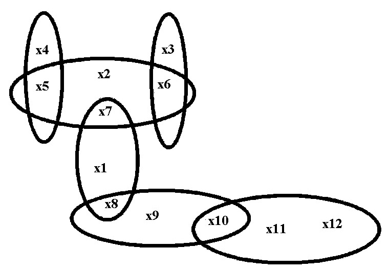
Figure 1: Hypergraph $H_{1}$ - graphical representation.

Removal, called also direct difference, is an ”inverse” operation to the combination. Formally, it can be defined as a mapping $\mbox{$\bigcirc\mbox{\rm R}\,$}:\mbox{{$\cal V$}}\times(\mbox{{$\cal N$}}\cup\mbox{{$\cal Z$}})\rightarrow\mbox{{$\cal N$}}\cup\mbox{{$\cal Z$}}$, that satisfies the three axioms:

(R1)

If $\sigma\in\mbox{{$\cal V$}}_{s}$ and $\rho\in\mbox{{$\cal N$}}_{r}\cup\mbox{{$\cal Z$}}_{r}$ then $\sigma\mbox{$\bigcirc\mbox{\rm R}\,$}\rho\in\mbox{{$\cal N$}}_{r\cup s}\cup\mbox{{$\cal Z$}}_{r\cup s}$.

(R2)

For each $\rho\in\mbox{{$\cal N$}}_{r}\cup\mbox{{$\cal Z$}}_{r}$ and for each $r\subseteq\mbox{{$\cal X$}}$ there exists an identity $\iota_{r}$ such that $\rho\mbox{$\bigcirc\mbox{\rm R}\,$}\rho=\iota_{r}$ .

(CR)

If $\sigma,\tau\in\mbox{{$\cal V$}}$ and $\rho\in\mbox{{$\cal N$}}\cup\mbox{{$\cal Z$}}$ then $(\sigma\otimes\tau)\mbox{$\bigcirc\mbox{\rm R}\,$}\rho=\sigma\otimes(\tau\mbox{$\bigcirc\mbox{\rm R}\,$}\rho)$.

Note that we can define the (pseudo)-inverse of a normal valuation by setting $\rho^{-1}=\iota_{\emptyset}\mbox{$\bigcirc\mbox{\rm R}\,$}\rho$. The main properties of removal are summarized in Lemma 2 given below.

Lemma 2

[?]. Suppose that $\sigma,\tau\in\mbox{{$\cal V$}}$and $\rho\in\mbox{{$\cal N$}}\cup\mbox{{$\cal Z$}}$. Then:

1. $(\sigma\otimes\tau)\mbox{$\bigcirc\mbox{\rm R}\,$}\rho=(\sigma\mbox{$\bigcirc\mbox{\rm R}\,$}\rho\otimes\tau)\otimes\tau$.

2. If $\sigma\in\mbox{{$\cal V$}}_{s}$ and $r\subseteq s$, then $\sigma\mbox{$\bigcirc\mbox{\rm R}\,$}\iota_{r}=\sigma\otimes\iota_{\emptyset}=\sigma$.

3. $[(\sigma\otimes\rho)\mbox{$\bigcirc\mbox{\rm R}\,$}\rho]\otimes\rho=\sigma\otimes\rho$.

4. $\rho^{-1}\otimes\rho=\rho\otimes\rho^{-1}$.

5. $\sigma\mbox{$\bigcirc\mbox{\rm R}\,$}\rho=\sigma\otimes\rho^{-1}$.

The propagation algorithm

With the concepts already introduced we define a VBS as a 5-tuple $(\mbox{{$\cal X$}},\mbox{\bf S},(\sigma_{s})_{s\in\mbox{\bf S}},\otimes,\downarrow)$, where S  is a family of subsets of the set of variables $\cal X$. The aim of uncertain reasoning is to find a marginal valuation

$$\rho=(\otimes{\sigma_{s}|s\in\mbox{\bf S}})^{\downarrow r},r\subseteq s,s\in\mbox{\bf S}.$$ (1)

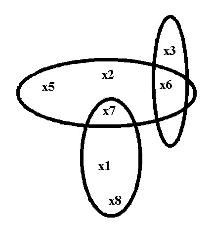
Figure 2: Subgraph of hypergraph $H_{1}$ from Fig. 1 for answering query $q$.

To apply the method of local computations, called the message-passing algorithm (MPA, for brevity) observe first that ($\cal X$, S) is nothing but a hypergraph. With this hypergraph we associate so-called Markov tree T = (H,E) i.e. a hypertree, or acyclic hypergraph, ($\cal X$, H), being a covering of ($\cal X$, S) and organized in a tree structure - see [?] for details. We say that ($\cal X$, H) covers ($\cal X$, S) if for each $s$ in S  there exists $h$ in H  such that $s\subseteq h$. Now if ($\cal X$, H) is a hypertree if it can be reduced to the empty set by recursively: 1) deleting vertices which are only in one edge, and 2) deleting hyperedges which are subsets of other hyperedges. These two steps define so-called Graham’s test. The sequence of hyperedge deletion determines a tree construction sequence (i.e. a set of undirected edges E) for a Markov tree T. Let us consider e.g. the hypergraph $H_{1}=\{\{X_{1},X_{7},X_{8}\},\{X_{2},X_{5},X_{6},X_{7}\},\{X_{3},X_{6}\},$ $\{X_{4},X_{5}\},$ $\{X_{8},X_{9},X_{10}\},\{X_{10},X_{11},X_{12}\}\}$ (see Fig.1). We see that variables $X_{1},X_{3},X_{4},X_{11},X_{12}$ are contained in only one edge. We delete them getting the hypergraph $H_{1}^{\prime}=\{\{X_{7},X_{8}\},\{X_{2},X_{5},X_{6},X_{7}\},$ $\{X_{6}\},$ $\{X_{5}\},$ $\{X_{8},X_{9},X_{10}\},\{X_{10}\}\}$. But then hyperedges $\{X_{6}\}$ and $\{X_{5}\}$ are contained in $\{X_{2},X_{5},X_{6},X_{7}\}$, and $\{X_{10}\}$ in $\{X_{8},X_{9},X_{10}\}$. So we delete them getting $H_{1}^{\prime\prime}=\{\{X_{7},X_{8}\},\{X_{2},X_{5},X_{6},X_{7}\},\{X_{8},X_{9},X_{10}\}\}$. Now variables $X_{2},X_{5},X_{6},$ $X_{9},X_{10}$ are contained in only one edge each. We get $H_{1}^{\prime\prime\prime}=\{\{X_{7},X_{8}\},$ $\{X_{7}\},\{X_{8}\}\}$. Now hyperedge $\{X_{7},X_{8}\}$ contains both $\{X_{7}\}$ and $\{X_{8}\}$, hence we get finally $H_{1}^{\prime\prime\prime\prime}=\{\{X_{7},X_{8}\}\}$, as the result of the Graham test which indicates that $H_{1}$ is a hypertree.

Now, the message passing algorithm can be summarized as follows: it tells the nodes of a Markov tree in what sequence to send their messages to propagate the local information throughout the tree. The algorithm is defined by two parts: a fusion rule, which describes how incoming messages are combined to make marginal valuations and outgoing messages for each node; and a propagation algorithm, which describes how messages are passed from node to node so that all of the local information is globally distributed. Just as propagation takes place along the edges of the tree, fusion takes place within the nodes. It is important to notice that in fact the MPA coincides with the two steps determining the tree construction sequence (i.e. Graham’s test).

3 Computing marginals in a Markov tree

Assume that we have constructed a Markov T = (H,E) tree representative of a given VBS, and let us assign a unique number $i\in I=\{1,2,...,n\}$, $n=$Card(H), to each node in the tree. Denote $V_{i}$ the original valuation stored in the $i$-th node of the tree, and $R_{j}$ the resultant valuation computed for $j$-th node according to the rule (1). Following [?] this $R_{j}$ is computed due to the rule

$$R_{j}=V_{j}\otimes(\otimes\{M_{i\rightarrow j}|i\in N(j)\})^{\downarrow j}$$ (2)

where $N(j)$ stands for the set of neighbours of the node $j$ in the Markov tree, $\downarrow j$ means marginalization to the set of variables corresponding to the node $j$, and $M_{i\rightarrow j}$ is the message sent by node $i$ to the node j calculated according to the equation (3)

$$M_{i\rightarrow j}=(V_{i}\otimes(\otimes\{M_{k\rightarrow i}|k\in(N(i)-\{j\})\}))^{\downarrow j}$$ (3)

It is obvious, that to find $R_{j}$ we place the node j in the root of the Markov tree and we move successively from leaves of the tree to its root. Note that if k is a leaf node and $\iota$ is its neighbour, then $M_{k\rightarrow i}=(V_{k})^{\downarrow i}$, hence (2) and (3) are defined properly.

A disadvantage of this algorithm is such that we can compute marginals for sets contained in the family H, or for subsets of these sets only. To find marginal for a any subset of variables we need a more elaborated approach. This problem was studied firstly by Xu [?]. Below we present its more economical modification.

First of all we need a generalization of a set chain representation, which has the next form under probabilistic context [?]: For a given tree construction sequence $\{h_{1},h_{2},...,h_{2}\}$ by a separator we understand a set $s_{i}$ such that $s_{i}=h_{i}\cap(h_{1}\cup h_{2}\cup...\cup h_{i-1})$. Separators are easily identified in a Markov tree, namely if $\{h_{i},h_{j}\}\in\mbox{\bf E}$ then $s_{i}=h_{i}\cap h_{j}$. Now, with given tree construction sequence the joint probability distribution can be represented as follows

$$P(x_{1},x_{2},...,x_{n})=R_{1}\prod\{(R_{i}/S_{i})|i=2,...,n\}$$ (4)

where $R_{i}$ and $S_{i}$ are the marginal probabilities defined over the set of variables represented by the sets $h_{i}$ and $s_{i}$, respectively. It appears, that for all VBS’s this property can be nicely extended, as we can see below. First we prove a lemma on an important property of VBS removal operator

Lemma 3

In Valuation-Based Systems, the following property of removal operator holds:

$$(\rho\mbox{$\bigcirc\mbox{\rm R}\,$}\rho^{\downarrow r})\otimes\rho^{\downarrow r}=\rho$$

PROOF:

From CM2: $\rho\otimes\iota_{\emptyset}=\rho$.From CR: $(\rho\otimes\iota_{\emptyset})\mbox{$\bigcirc\mbox{\rm R}\,$}\rho^{\downarrow r}=\rho\otimes(\iota_{\emptyset}\mbox{$\bigcirc\mbox{\rm R}\,$}\rho^{\downarrow r})$. But by definition: $\iota_{\emptyset}\mbox{$\bigcirc\mbox{\rm R}\,$}\rho^{\downarrow r}=(\rho^{\downarrow r})^{-1}$, hence $(\rho\mbox{$\bigcirc\mbox{\rm R}\,$}\rho^{\downarrow r})\otimes\rho^{\downarrow r}=(\rho\otimes(\rho^{\downarrow r})^{-1})\otimes\rho^{\downarrow r}$. From C2 $(\rho\otimes(\rho^{\downarrow r})^{-1})\otimes\rho^{\downarrow r}=\rho\otimes((\rho^{\downarrow r})^{-1}\otimes\rho^{\downarrow r})$.But we know that: From R2 $\rho\mbox{$\bigcirc\mbox{\rm R}\,$}\rho=\iota_{\rho}$. From CM2 $(\rho\otimes\iota_{\emptyset})\mbox{$\bigcirc\mbox{\rm R}\,$}\rho=\iota_{\rho}$. From CR $\rho\otimes(\iota_{\emptyset}\mbox{$\bigcirc\mbox{\rm R}\,$}\rho)=\iota_{\rho}$. hence $\rho\otimes\rho^{-1}=\iota_{\rho}$.Therefore $\rho\otimes((\rho^{\downarrow r})^{-1}\otimes\rho^{\downarrow r})=\rho\otimes\iota_{\rho^{\downarrow r}}$.So we get due to axiom CM2 $\rho\otimes\iota_{\rho^{\downarrow r}}=\rho$.which proves our claim. $\mbox{Q.e.d.}\Box$

Now let us try to transform a Markov tree valuation to the form similar to equation (4).

Assume that we have constructed a Markov tree T = (H,E) representative of a given VBS, and let us assign a unique number $i\in I=\{1,2,...,n\}$, $n=$Card(H), to each node in the tree. Denote $V_{i}$ the original valuation stored in the $i$-th node of the tree. Let us consider the following transformation algorithm: starting with the node $k$=$n$ down to $1$ we run a ”valuation move” step such that we will ”move” valuation from nodes with smaller number $i$ to ones with higher one so that final valuation stored in the $k$-th node of the tree will be $R_{k}\mbox{$\bigcirc\mbox{\rm R}\,$}S_{k}$, where $R_{k}$ and $S_{k}$ are the marginal valuations defined over the set of variables represented by the sets $h_{k}$ and $s_{k}$, respectively. Each step is a kind of unidirectional message-passing (towards the actual node $k$) in that a message is calculated at a node and then (1) removed from the valuation of the node and (2) added to the node closer to $k$. The valuation of nodes $i=1,...,k$ at the beginning of step concerning node $k$ is denoted with $V_{i,k}$. At the end of a step, the valuation is denoted with $V_{i,k-1}$ except for node $k$ which is denoted with $R_{k}\mbox{$\bigcirc\mbox{\rm R}\,$}S_{k}$

The Algorithm:

begin

1. for $k:=n$ step -1 downto 1 $V_{k,n}$:= $V_{k}$

2. for k:=n step -1 downto 2
   begin

   1. Construct a subtree $\Gamma_{k}=(\mbox{\bf H}_{k},\mbox{\bf E}_{k})$ of T consisting only of nodes $\mbox{\bf H}_{k}=\{1,...,k\}$.

   2. Introduce the order $<_{k}$ compatible with the tree $\Gamma_{k}$, but such that the node $k$ is considered as its root (the smallest element in $<_{k}$).

   3. Mark all nodes of the $\Gamma_{k}$ inactive

   4. while the the direct successor of node $k$ in ordering $<_{k}$ inactive
      if, in ordering $<_{k}$, all direct successors of node $i$ are active, then:
      begin

      1. Active node $i$

      2. Denote all its direct successors as inactive

      3. Let $j$ be direct predecessor of $i$ in $<_{k}$

      4. Calculate

         $$V^{\prime}_{i,k}:=(V_{i,k}\otimes(\otimes\{M_{l\rightarrow i}|l\in(N(i)_{k}-\{j\}\})$$

         $$M_{i\rightarrow j}:={V^{\prime}_{i,k}}^{\downarrow j\cap i}$$

         If $(i,k)\not\in\mbox{\bf E}_{k}$ calculate:

         $$V_{i,k-1}:=V^{\prime}_{i,k}\mbox{$\bigcirc\mbox{\rm R}\,$}M_{i\rightarrow j}$$

         where $N(i)_{k}$ stands for the set of neighbours of the node $i$ in the Markov subtree $\Gamma_{k}$,

      end

   5. Let $k+$ denote the direct successor of node $k$ in $<_{k}$
      Calculate

      $$R_{k}:=V_{k,k}\otimes M_{k+\rightarrow k}$$

      $$S_{k}:=R_{k}^{\downarrow k\cap k+}$$

      $$V_{k+,k-1}:=(V^{\prime}_{k+,k}\mbox{$\bigcirc\mbox{\rm R}\,$}M_{k+\rightarrow k})\otimes S_{k}$$

   end

3. Calculate $R_{1}:=V_{1,1}$

end

THEOREM 4

If $R_{i}$ and $S_{i}$ have been calculated by the above algorithm for the Markov tree T, then

$$R=\otimes\{V_{i}|i=1..n\}=$$

$$=R_{1}\otimes(\otimes\{(R_{i}\mbox{$\bigcirc\mbox{\rm R}\,$}S_{i})|i=2..n\})$$

where $R$ stands for the joint valuation defined over $\cal X$.

PROOF:

In any subtree $\Gamma_{k}$ for any node $i$ with predecessor $j$ in $<_{k}$ except $k$ and $k+$ we have, due to Lemma 3

$$V_{i,k}\otimes(\otimes\{V^{\prime}_{l,k}|l\in(N(i)_{k}-\{j\}\})=$$

$$=V_{i,k}\otimes(\otimes\{V_{l,k-1}\otimes M_{l\rightarrow i}|l\in(N(i)_{k}-\{j\}\})=$$

$$=V^{\prime}_{i,k}\otimes(\otimes\{V_{l,k-1}|l\in(N(i)_{k}-\{j\}\})$$

hence update on passage of activation does not change the joint valuation.
Also we have that

$$V^{\prime}_{k+,k}\otimes V_{k,k}=(V^{\prime}_{k+,k}\mbox{$\bigcirc\mbox{\rm R}\,$}M_{k+\rightarrow k})\otimes(V_{k,k}\otimes M_{k+\rightarrow k})=$$

$$=(V^{\prime}_{k+,k}\mbox{$\bigcirc\mbox{\rm R}\,$}M_{k+\rightarrow k})\otimes R_{k}=$$

$$=((V^{\prime}_{k+,k}\mbox{$\bigcirc\mbox{\rm R}\,$}M_{k+\rightarrow k})\otimes S_{k})\otimes(R_{k}\mbox{$\bigcirc\mbox{\rm R}\,$}S_{k})=$$

$$=V_{k+,k-1}\otimes(R_{k}\mbox{$\bigcirc\mbox{\rm R}\,$}S_{k})$$

The theorem is then provable by induction (on k running from n to 1)

$\mbox{Q.e.d.}\Box$

THEOREM 5

In the previous theorem, $R_{i}=R^{\downarrow h_{i}}$

PROOF:

It is easily seen that $R_{k}$ is always the projection of the joint valuation of the subtree $\Gamma_{k}$ (compare the message passing algorithm of Shenoy and Shafer [?]). Hence especially $R_{n}$ is the projection of $R$ onto node $n$.
Further, let $R_{\Gamma_{k}}=V^{\prime}_{k,k}\times(\otimes\{V_{i,k}|i=1,2,...,k-1\}$ Then, due to CM1 we have: $R_{\Gamma_{k-1}}=R_{\Gamma_{k}}^{1\cup 2\cup....\cup k-1}$. This implies, by induction, that $R_{k}$ is the projection of $R$ onto node $k$ for every $k=1,2,...,n$.

$\mbox{Q.e.d.}\Box$

These two theorems 4, 5 may be summarized as follows.

THEOREM 6

Let T = (H,E) be a Markov representative of a VBS $(\mbox{{$\cal X$}},\mbox{\bf S},(\sigma_{s})_{s\in\mbox{\bf S}},\otimes,\downarrow)$. Let $R_{i}$ stands for the valuation marginalized to the set $v_{i}$ of variables and $S_{j}$ stands for the marginal potential assigned to the separator of the pair $\{h_{i},h_{j}\}$. Then

$$R=\otimes\{V_{i}|i=1..n\}=R_{1}\otimes(\otimes\{(R_{i}\mbox{$\bigcirc\mbox{\rm R}\,$}S_{i})|i=2..n\})$$

where $R$ stands for the joint valuation defined over $\cal X$.

Note that this theorem and the subsequent one are generalizations of theorems presented by Wierzchoń, [?], in that the restricting condition that the removal operation has to satisfy the property $(\rho\otimes\sigma)\mbox{$\bigcirc\mbox{\rm R}\,$}(\delta\otimes\sigma)=(\rho\mbox{$\bigcirc\mbox{\rm R}\,$}\delta)$ for any normal valuations $\rho,\sigma$ and $\delta$ has been dropped. They represent also generalizations of properties of Dempster-Shafer belief functions presented in [?] and [?].

With the theorem 6 we can easily compute join valuations for subsets being set theoretical union of members of the family H. This fact presents Theorem 7 below.

THEOREM 7

Let $\Gamma=(\mbox{\bf N},\mbox{\bf F})$ be a subtree of a Markov tree T = (H, E) satisfying assumptions of Theorem 6 Assume that for each node $h_{j}\in\mbox{\bf H}$ the marginal valuation, $R_{j}$, has been already computed. If $h_{r}$ stands for the root node in the subtree $\Gamma$ then

$$R^{\downarrow\cup\mbox{\bf N}}=\otimes\{V_{i}|i\in\mbox{\bf H}\}^{\downarrow\cup\mbox{\bf N}}=$$

$$=R_{r}\otimes(\otimes\{(R_{i}\mbox{$\bigcirc\mbox{\rm R}\,$}S_{i})|i\in\mbox{\bf N}-\{v_{r}\})\}$$

where $\cup\mbox{\bf N}$ stands the set theoretical union of all sets contained in N.

PROOF:

The result is straight-forward if we recall the axiom CM1 and the separator property of the Markov tree. $\mbox{Q.e.d.}\Box$

Now, if $h\subseteq\cup\mbox{\bf N}$ then $R^{\downarrow h}$ is computed as $(R^{\downarrow\cup\mbox{\bf N}})^{\downarrow h}$. Xu [?] proposed the local computation technique to find such a marginal: it is simple consequence of Theorem 7 above and of Lemma 2.5 in [?].

4 Query processing in VBS

The problem of query processing was formulated by Pearl [?] first. In this approach we modify the original Bayesian belief network by adding new nodes with appropriate edges. Consider for instance the query $q=(x_{1}\land x_{2})\lor x_{3}$ - see ([?], p. 224). Obviously, this $q$ introduces new subset $h=\{x_{1},x_{2},x_{3}\}$ to H. In Pearl’s approach we add two additional nodes joined to the original network by three edges.

This approach suffers from several disadvantages. Adding new nodes to a belief network may change, even radically, the structure of the corresponding hypergraph which makes reconstruction of the Markov tree necessary, which is time-consuming. In the process, also Markov tree may change radically and practically all valuations have to be recalculated.

In practice, query $q$ may be frequently expressed in form of a single conjunction of elementary (that is mutually exclusive) expressions or a disjunction of a few conjunctions. E.g.: the query $q=(x_{1}\land x_{2})\lor x_{3}$ may be restated as $q=(x_{1}\land x_{2}\land\lnot x_{3})\lor x_{3}$ where conjuctions $(x_{1}\land x_{2}\land\lnot x_{3})$ and $x_{3}$ are mutually exclusive. It can be shown that calculation of such a query can be done without modification of Markov tree. Under probabilistic settings as well as in DST, if $A$ and $B$ are mutually excluding conditions then $\rho(A\lor B)=\rho(A)+\rho(B)$. (In our example: $\rho((x_{1}\land x_{2}\land\lnot x_{3})\lor x_{3})=\rho(x_{1}\land x_{2}\land\lnot x_{3})+\rho(x_{3})$. Therefore, in our approach we must simply compute ${R}^{\downarrow h}$ (with $h$ being the set of variables appearing in the query $q$), and next we should find valuations over the set of configurations logically equivalent to $q$. In our example we find valuation first for configuration: $X_{1}=true,X_{2}=true,X_{3}=false,$ universe value for other variables, and then for configuration $X_{3}=true,$ universe value for other variables.

The only problem is to find the subtree $\Gamma$ with $h\subseteq\cup\mbox{\bf N}$. In [?] it was shown that the minimal subtree, in the sense that $\cup\mbox{\bf N}$ is as small as possible, can be found by applying modified Graham’s test. The modification concerns step (1) of this test: a variable is deleted only if it does not belong to the set $h$.

Consider e.g. again the hypergraph $H_{1}=$$\{\{X_{1},X_{7},X_{8}\},\{X_{2},X_{5},X_{6},X_{7}\},\{X_{3},X_{6}\},$ $\{X_{4},X_{5}\},$$\{X_{8},X_{9},X_{10}\},\{X_{10},X_{11},X_{12}\}\}$ (see Fig.1). We see that variables $X_{1},X_{3},$ $X_{4},X_{11},$ $X_{12}$ are contained in only one edge, but $X_{1},X_{3}$ are in $h$. We delete only the other getting the hypergraph $H_{1}^{\prime}=\{\{X_{1},X_{7},X_{8}\},$ $\{X_{2},X_{5},X_{6},X_{7}\},$ $\{X_{3},X_{6}\},$ $\{X_{5}\},$ $\{X_{8},X_{9},X_{10}\},$ $\{X_{10}\}\}$. But then hyperedge $\{X_{5}\}$ is contained in $\{X_{2},X_{5},X_{6},X_{7}\}$, and $\{X_{10}\}$ in $\{X_{8},X_{9},X_{10}\}$. So we delete them getting $H_{1}^{\prime\prime}=\{\{X_{1},X_{7},X_{8}\},\{X_{2},X_{5},X_{6},X_{7}\},\{X_{3},X_{6}\}$ $,\{X_{8},X_{9},X_{10}\}\}$. Now variables $X_{2},X_{5},X_{9},X_{10}$ are contained in only one edge each, however $X_{2}$ is in $h$. We get $H_{1}^{\prime\prime\prime}=\{\{X_{1},X_{7},X_{8}\},$ $\{X_{2},X_{6},X_{7}\},$ $\{X_{3},X_{6}\},$ $\{X_{8}\}\}$. Now hyperedge $\{X_{1},X_{7},X_{8}\}$ contains $\{X_{8}\}$, hence we get $H_{1}^{\prime\prime\prime\prime}=\{\{X_{1},X_{7},X_{8}\},$ $\{X_{2},X_{6},X_{7}\},$ $\{X_{3},X_{6}\}\}$. $X_{8}$ appears only in one edge, so we get finally $H_{1}^{\prime\prime\prime\prime\prime}=\{\{X_{1},X_{7}\},$ $\{X_{2},X_{6},X_{7}\},$ $\{X_{3},X_{6}\}\}$. No further reduction by modified Graham test is possible. We conclude that out of 6 hyperedges of $H_{1}$ only three $\{X_{1},X_{7},X_{8}\},\{X_{2},X_{5},X_{6},X_{7}\},\{X_{3},X_{6}\}$ are necessary for query answering calculations (see Fig.2), and that $\{X_{2},X_{5},X_{6},X_{7}\}$ may be projected to $\{X_{2},X_{6},X_{7}\}$, and $\{X_{1},X_{7},X_{8}\}$ onto $\{X_{1},X_{7}\}$.

This procedure is much more effective than that one suggested by Xu [?], because this last method heavily depends on the topology of a Markov tree.

We can, however, pose the question, whether or not the optimal subtree of the Markov tree T = (H, E) with hypertree H  covering an original hypergraph S would be ”better” for query answering than an optimal hypertree cover T’ = (H’, E’) of the result of the above-mentioned modified Graham test run over the original hypergraph S. The answer to this question is rather ambiguous. We can clearly construct examples where T’ would be more optimal than the subtree T in terms e.g. of the maximum number of nodes in an edge. However, we must take into account that for each query not only T’ but also the valuation for each node of the tree T’ has to be calculated from the entire hypergraph S. But we do not need to do that with subtrees of T, because we have to calculate the $R_{j}$’s for a given tree T once and we do not need to recalculate them when selecting a subtree, and if the subtree is small enough we save much calculation compared with processing of T’ (even if T’ has a more optimal structure for a given query).

Concluding this paper we want to stress that this approach is implemented in the VBS system designed by our group.

References

- [1972] U. Bertele and F. Brioschi. Nonserial Dynamic Programming. Academic Press, NY, 1972.
- [1961] A.H. Clifford and G.B. Preston. The Algebraic Theory of Semigroups. American Mathematical Society, Providence, Rhode Island, vol. 1, (1961)
- [1992] G.F. Cooper and E. Herskovits. A Bayesian method for the induction of probabilistic networks from data. Machine Learning, 9:309-347, 1992.
- [1990] F.V. Jensen, S.L. Lauritzen, and K.G. Olesen. Bayesian updating in causal probabilistic networks by local computations. Computational Statistics Quarterly, 4: 269-282, 1990.
- [1994] M.A. Kłopotek. Beliefs in Markov Trees - From Local Computations to Local Valuation. in: R. Trappl, ed.: Proc. EMCSR’94 Vol.1. pages 351-358, 1994.
- [1995] M.A. Kłopotek. On (Anti)Conditional Independence in Dempster-Shafer Theory to appear in Journal Mathware and Softcomputing, 1995.
- [1988] S.L. Lauritzen and D.J. Spiegelhalter. Local computation with probabilities on graphical structures and their application to expert systems. J. Roy. Stat. Soc., B50: pages 157-244, 1988.
- [1988] J. Pearl. Probabilistic Reasoning in Intelligent Systems: Networks of Plausible Inference. Morgan Kaufman, 1988.
- [1976] G. Shafer. A Mathematical Theory of Evidence. Princeton University Press, Princeton, NJ, 1976.
- [1989] P.P. Shenoy. A valuation-based language for expert systems. International Journal of Approximate Reasoning, 3:383-411, 1989.
- [1991] P.P. Shenoy. Valuation-based systems for discrete optimization. in P.P. Bonissone, M. Henrion, L.N. Kanal and J.F. Lemmer, eds: Uncertainty in Artificial Intelligence 6, North-Holland, Amsterdam, pages 385-400, 1991.
- [1993] P.P. Shenoy. A new method for representing and solving Bayesian decision problems. in D.J. Hand, ed.: Artificial Intelligence Frontiers in Statistics: AI and Statistics III , Chapman & Hall, London, pages 119-138, 1993.
- [1994] P.P. Shenoy. Conditional independence in valuation-based systems. International Journal of Approximate Reasoning, 10:203-234, 1994.
- [1986] P.P. Shenoy and G. Shafer. Propagating belief functions using local computations. IEEE Expert, 1(3), pages 43-52, 1986.
- [1991] H.M. Thoma. Belief function computations. in: I.R. Goodman et al (Eds.): Conditional Logics in Expert Systems, North-Holland, pages 269-308, 1991.
- [1991] W.X. Wen. From relational databases to belief networks, in: B.D’Ambrosio, Ph. Smets, and P.P. Bonissone (Eds.), Proc. 7-th Conference on Uncertainty in Artificial Intelligence, Morgan Kaufmann, pages 406-413, 1991.
- [1995] S.T. Wierzchoń. Markov-like properties of joint valuations, submitted, 1995.
- [1993] S.K. Wong, Y. Xiang, and X. Nie. Representation of Bayesian networks as relational databases. in: D. Heckerman, and A. Mamdani, (Eds.), Proc. 9-th Conference on Uncertainty in Artificial Intelligence, Morgan Kaufmann, pages 159-165, 1993.
- [1995] H. Xu. Computing marginals for arbitrary subsets from marginal representation in Markov trees. Artificial Intelligence, 74, pages 177-189, 1995.