Compact Trilinear Interaction for Visual Question Answering

Abstract

In Visual Question Answering (VQA), answers have a great correlation with question meaning and visual contents. Thus, to selectively utilize image, question and answer information, we propose a novel trilinear interaction model which simultaneously learns high level associations between these three inputs. In addition, to overcome the interaction complexity, we introduce a multimodal tensor-based PARALIND decomposition which efficiently parameterizes trilinear interaction between the three inputs. Moreover, knowledge distillation is first time applied in Free-form Opened-ended VQA. It is not only for reducing the computational cost and required memory but also for transferring knowledge from trilinear interaction model to bilinear interaction model. The extensive experiments on benchmarking datasets TDIUC, VQA-2.0, and Visual7W show that the proposed compact trilinear interaction model achieves state-of-the-art results when using a single model on all three datasets. The source code is available at https://github.com/aioz-ai/ICCV19_VQA-CTI.

1 Introduction

The aim of VQA is to find out a correct answer for a given question which is consistent with visual content of a given image [25, 3, 10]. There are two main variants of VQA which are Free-Form Opened-Ended (FFOE) VQA and Multiple Choice (MC) VQA. In FFOE VQA, an answer is a free-form response to a given image-question pair input, while in MC VQA, an answer is chosen from an answer list for a given image-question pair input.

Traditional approaches to both VQA tasks mainly aim to learn joint representations between images and questions, while the answers are treated in a “passive” form, i.e., the answers are only considered as classification targets. However, an answer is expected to have high correlation with its corresponding question-image input, hence a jointly and explicitly information extraction from these three inputs will give a highly meaningful joint representation. In this paper, we propose a novel trilinear interaction model which simultaneously learns high level associations between all three inputs, i.e., image, question, and answer.

The main difficulty in trilinear interaction is the dimensionality issue which causes expensive computational cost and huge memory requirement. To tackle this challenge, we propose to use PARALIND decomposition [6] which factorizes a large tensor into smaller tensors which reduces the computational cost and the usage memory.

The proposed trilinear interaction takes images, questions and answers as inputs. However, answer information in FFOE VQA [1, 40, 26, 39] is only available in the training phase but not in the testing phase. To apply the trilinear interaction for FFOE VQA, we propose to use knowledge distillation to transfer knowledge from trilinear model to bilinear model. The distilled bilinear model only requires pairs of image and question as inputs, hence it can be used for the testing phase. For MC VQA [47, 19, 27, 15, 30, 44], the answer information can be easily extracted, thanks to the given answer list that contains few candidate answers for each image-question pair and is available in both training and testing phases. Thus, the proposed trilinear interaction can be directly applied to MC VQA.

To evaluate the effectiveness of the proposed model, the extensive experiments are conducted on the benchmarking datasets TDIUC, VQA-2.0, and Visual7W. The results show that the proposed model achieves state-of-the-art results on all three datasets.

The main contributions of the paper are as follows. (i) We propose a novel trilinear interaction model which simultaneously learns high level joint presentation between image, question, and answer information in VQA task. (ii) We utilize PARALIND decomposition to deal with the dimensionality issue in trilinear interaction. (iii) To make the proposed trilinear interaction applicable for FFOE VQA, we propose to use knowledge distillation for transferring knowledge from trilinear interaction model to bilinear interaction model. The remaining of this paper is organized as follows. Section 2 presents the related work. Section 3 presents the proposed compact trilinear interaction (CTI). Section 4 presents the proposed models when applying CTI to FFOE VQA and MC VQA. Section 5 presents ablation studies, experimental results and analysis.

2 Related Work

Joint embedding in Visual Question Answering. There are different approaches have been proposed for VQA [18, 5, 8, 45, 20, 42, 24, 2, 28, 23, 38, 46, 29, 40]. Most of the successful methods focus on learning joint representation between the input question and image [8, 5, 18, 45]. In the state-of-the-art VQA, the features of the input image and question are usually represented under matrix forms. E.g., each image is described by a number of interested regions, and each region is represented by a feature vector. Similar idea is applied for question, e.g., an question contains a number of words and each word is represented by a feature vector. A fully expressive interaction between an image region and a word should be the outer product between their two corresponding vectors [8]. The outer product allows a multiplicative interaction between all elements of both vectors. However, a fully bilinear interaction using outer product between every possible pairs of regions and words will dramatically increase the output space. Hence instead of directly computing the fully bilinear with outer product, most of works try to compress or decompose the fully bilinear interaction.

In [8], the authors proposed the Multimodal Compact Bilinear pooling which is an efficient method to compress the bilinear interaction. The method works by projecting the visual and linguistic features to a higher dimensional space and then convolving both vectors efficiently by using element-wise product in Fast Fourier Transform space. In [5], the authors proposed Multimodal Tucker Fusion which is a tensor-based Tucker decomposition to efficiently parameterize bilinear interaction between visual and linguistic representations. In [45], the author proposed Factorized Bilinear Pooling that uses two low rank matrices to approximate the fully bilinear interaction. Recently, in [18] the authors proposed Bilinear Attention Networks (BAN) that finds bilinear attention distributions to utilize given visual-linguistic information seamlessly. BAN also uses low rank approximation to approximate the bilinear interaction for each pair of vectors from image and question.

There are other works that consider answer information, besides image and question information, to improve VQA performance [16, 9, 36, 14, 41, 34]. Typically, in [14], the authors learned two embedding functions to transform an image-question pair and an answer into a joint embedding space. The distance between the joint embedded image-question and the embedded answer is then measured to determine the output answer. In [41], the authors computed joint representations between image and question, and between image and answer. They then learned a joint embedding between the two computed representations.

In [34], the authors computed “ternary potentials” which capture the dependencies between three inputs, i.e., image, question, and answer. For every triplet of vectors, each from each different input, to compute the interaction between three vectors, instead of calculating the outer products, the author computed the sum of element-wise product of the three vectors. This greatly reduces the computational cost but it might not be expressive enough to fully capture the complex associations between the three vectors.

Different from previous works that mainly aim to learn the joint representations from pairs of modalities [8, 5, 18, 45, 14, 41] or greatly simplify the interaction between the three modalities by using the element-wise operator [34], in this paper, we propose a principle and direct approach – a trilinear interaction model, which simultaneously learns a joint representation between three modalities. In particular, we firstly derive a fully trilinear interaction between three modalities. We then rely on a decomposition approach to develop a compact model for the interaction.

Knowledge Distillation. Knowledge Distillation is a general approach for transferring knowledge from a cumbersome model (teacher model) to a lighten model (student model) [13, 11, 33, 7, 4]. In FFOE VQA, the trilinear interaction model, which takes image, question, and answer as inputs, can only be applied for training phase but not for testing phase due to the omission of answer in testing. To overcome this challenge and also to reduce computational cost, inspired from the Hinton’s seminar work [13], we propose to use knowledge distillation to transfer knowledge from trilinear model to bilinear model.

3 Compact Trilinear Interaction (CTI)

3.1 Fully parameterized trilinear interaction

Let $M=\{M_{1},M_{2},M_{3}\}$ be the representations of three inputs. $M_{t}\in\mathds{R}^{n_{t}\times d_{t}}$, where $n_{t}$ is the number of channels of the input $M_{t}$ and $d_{t}$ is the dimension of each channel. For example, if $M_{1}$ is the region-based representation for an image, then $n_{1}$ is the number of regions and $d_{1}$ is the dimension of the feature representation for each region. Let $m_{t_{e}}\in\mathds{R}^{1\times d_{t}}$ be the $e^{th}$ row of $M_{t}$, i.e., the feature representation of $e^{th}$ channel in $M_{t}$, where $t\in\{1,2,3\}$.

The joint representation resulted from a fully parameterized trilinear interaction over the three inputs is presented by $z\in\mathds{R}^{d_{z}}$ which is computed as follows

$$z^{T}=\left(\left(\mathcal{T}\times_{1}vec(M_{1})\right)\times_{2}vec(M_{2})\right)\times_{3}vec(M_{3})$$ (1)

where $\mathcal{T}\in\mathds{R}^{d_{M_{1}}\times d_{M_{2}}\times d_{M_{3}}\times d_{z}}$ is a learning tensor; $d_{M_{t}}=n_{t}\times d_{t}$; $vec(M_{t})$ is a vectorization of $M_{t}$ which outputs a row vector; operator $\times_{i}$ denotes the $i$-mode tensor product.

The tensor $\mathcal{T}$ helps to learn the interaction between the three input through $i$-mode product. However, learning such a large tensor $\mathcal{T}$ is infeasible when the dimension $d_{M_{t}}$ of each input modality is high, which is the usual case in VQA. Thus, it is necessary to reduce the size $\mathcal{T}$ to make the learning feasible.

Inspired by [43], we rely on the idea of unitary attention mechanism. Specifically, let $z_{p}\in\mathds{R}^{d_{z}}$ be the joint representation of $p^{th}$ triplet of channels where each channel in the triplet is from a different input. The representation of each channel in a triplet is $m_{1_{i}},m_{2_{j}},m_{3_{k}}$, where $i\in[1,n_{1}],j\in[1,n_{2}],k\in[1,n_{3}]$, respectively. There are $n_{1}\times n_{2}\times n_{3}$ possible triplets over the three inputs. The joint representation $z_{p}$ resulted from a fully parameterized trilinear interaction over three channel representations $m_{1_{i}},m_{2_{j}},m_{3_{k}}$ of $p^{th}$ triplet is computed as

$$z_{p}^{T}=\left(\left(\mathcal{T}_{sc}\times_{1}m_{1_{i}}\right)\times_{2}m_{2_{j}}\right)\times_{3}m_{3_{k}}$$ (2)

where $\mathcal{T}_{sc}\in\mathds{R}^{d_{1}\times d_{2}\times d_{3}\times d_{z}}$ is the learning tensor between channels in the triplet.

Follow the idea of unitary attention [43], the joint representation $z$ is approximated by using joint representations of all triplets described in (2) instead of using fully parameterized interaction over three inputs as in (1). Hence, we compute

$$z=\sum_{p}\mathcal{M}_{p}z_{p}$$ (3)

Note that in (3), we compute a weighted sum over all possible triplets. The $p^{th}$ triplet is associated with a scalar weight $\mathcal{M}_{p}$. The set of $\mathcal{M}_{p}$ is called as the attention map $\mathcal{M}$, where $\mathcal{M}\in\mathds{R}^{n_{1}\times n_{2}\times n_{3}}$.

The attention map $\mathcal{M}$ resulted from a reduced parameterized trilinear interaction over three inputs $M_{1},M_{2}$ and $M_{3}$ is computed as follows

$$\mathcal{M}=\left(\left(\mathcal{T}_{\mathcal{M}}\times_{1}M_{1}\right)\times_{2}M_{2}\right)\times_{3}M_{3}$$ (4)

where $\mathcal{T}_{\mathcal{M}}\in\mathds{R}^{d_{1}\times d_{2}\times d_{3}}$ is the learning tensor of attention map $\mathcal{M}$. Note that the learning tensor $\mathcal{T}_{\mathcal{M}}$ in (4) has a reduced size compared to the learning tensor $\mathcal{T}$ in (1).

By integrating (2) into (3), the joint representation $z$ in (3) can be rewritten as

$$z^{T}=\sum_{i=1}^{n_{1}}\sum_{j=1}^{n_{2}}\sum_{k=1}^{n_{3}}\mathcal{M}_{ijk}\left(\left(\left(\mathcal{T}_{sc}\times_{1}m_{1_{i}}\right)\times_{2}m_{2_{j}}\right)\times_{3}m_{3_{k}}\right)$$ (5)

where $\mathcal{M}_{ijk}$ in (5) is actually a scalar attention weight $\mathcal{M}_{p}$ of the attention map $\mathcal{M}$ in (4).

It is also worth noting from (5) that to compute $z$, instead of learning the large tensor $\mathcal{T}\in\mathds{R}^{d_{M_{1}}\times d_{M_{2}}\times d_{M_{3}}\times d_{z}}$ in (1), we now only need to learn two smaller tensors $\mathcal{T}_{sc}\in\mathds{R}^{d_{1}\times d_{2}\times d_{3}\times d_{z}}$ in (2) and $\mathcal{T}_{\mathcal{M}}\in\mathds{R}^{d_{1}\times d_{2}\times d_{3}}$ in (4).

3.2 Parameter factorization

Although the large tensor $\mathcal{T}$ of trilinear interaction model is replaced by two smaller tensors $\mathcal{T}_{\mathcal{M}}$ and $\mathcal{T}_{sc}$, the dimension of these two tensors still large which makes the learning difficult. To further reduce the computational complexity, the PARALIND decomposition [6] is applied for $\mathcal{T}_{\mathcal{M}}$ and $\mathcal{T}_{sc}$. The PARALIND decomposition for the learning tensor $\mathcal{T}_{\mathcal{M}}\in\mathds{R}^{d_{1}\times d_{2}\times d_{3}}$ can be calculated as

$$\mathcal{T}_{\mathcal{M}}\approx\sum^{R}_{r=1}\left(\left(\mathcal{G}_{r}\times_{1}W_{1_{r}}\right)\times_{2}W_{2_{r}}\right)\times_{3}W_{3_{r}}$$ (6)

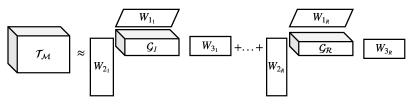
Figure 1: PARALIND decomposition for a tensor $\mathcal{T}_{\mathcal{M}}$.

where $R$ is a slicing parameter, establishing a trade-off between the decomposition rate (which is directly related to the usage memory and the computational cost) and the performance. Each $\mathcal{G}_{r}\in\mathds{R}^{d_{1_{r}}\times d_{2_{r}}\times d_{3_{r}}}$ is a smaller learnable tensor called Tucker tensor. The number of these Tucker tensors equals to $R$. The maximum value for $R$ is usually set to the greatest common divisor of $d_{1},d_{2}$ and $d_{3}$. In our experiments, we found that $R=32$ gives a good trade-off between the decomposition rate and the performance.

Here, we have dimension $d_{1_{r}}=d_{1}/R$, $d_{2_{r}}=d_{2}/R$ and $d_{3_{r}}=d_{3}/R$; $W_{1_{r}}\in\mathds{R}^{d_{1}\times d_{1_{r}}}$, $W_{2_{r}}\in\mathds{R}^{d_{2}\times d_{2_{r}}}$ and $W_{3_{r}}\in\mathds{R}^{d_{3}\times d_{3_{r}}}$ are learnable factor matrices. Figure 1 shows the illustration of PARALIND decomposition for a tensor $\mathcal{T}_{\mathcal{M}}$.

The shorten form of $\mathcal{T}_{\mathcal{M}}$ in (6) can be rewritten as

$$\mathcal{T}_{\mathcal{M}}\approx\sum^{R}_{r=1}{\llbracket\mathcal{G}_{r};W_{1_{r}},W_{2_{r}},W_{3_{r}}\rrbracket}$$ (7)

Integrating the learning tensor $\mathcal{T}_{\mathcal{M}}$ from (7) into (4), the attention map $\mathcal{M}$ can be rewritten as

$$\mathcal{M}=\sum^{R}_{r=1}{\llbracket\mathcal{G}_{r};M_{1}W_{1_{r}},M_{2}W_{2_{r}},M_{3}W_{3_{r}}\rrbracket}$$ (8)

Similar to $\mathcal{T}_{\mathcal{M}}$, PARALIND decomposition is also applied to the tensor $\mathcal{T}_{sc}$ in (5) to reduce the complexity. It is worth noting that the size of $\mathcal{T}_{sc}$ directly effects to the dimension of the joint representation $z\in\mathds{R}^{d_{z}}$. Hence, to minimize the loss of information, we set the slicing parameter $R=1$ and the projection dimension of factor matrices at $d_{z}$, i.e., the same dimension of the joint representation $z$.

Therefore, $\mathcal{T}_{sc}\in\mathds{R}^{d_{1}\times d_{2}\times d_{3}\times d_{z}}$ in (5) can be calculated as

$$\mathcal{T}_{sc}\approx\left(\left(\mathcal{G}_{sc}\times_{1}W_{z_{1}}\right)\times_{2}W_{z_{2}}\right)\times_{3}W_{z_{3}}$$ (9)

where $W_{z_{1}}\in\mathds{R}^{d_{1}\times d_{z}}$, $W_{z_{2}}\in\mathds{R}^{d_{2}\times d_{z}}$, $W_{z_{3}}\in\mathds{R}^{d_{3}\times d_{z}}$ are learnable factor matrices and $\mathcal{G}_{sc}\in\mathds{R}^{d_{z}\times d_{z}\times d_{z}\times d_{z}}$ is a smaller tensor (compared to $\mathcal{T}_{sc}$).

Up to now, we already have $\mathcal{M}$ by (8) and $\mathcal{T}_{sc}$ by (9), hence, we can compute $z$ using (5). $z$ from (5) can be rewritten as

$$z^{T}=\sum_{i=1}^{n_{1}}\sum_{j=1}^{n_{2}}\sum_{k=1}^{n_{3}}$$ (10)

$$\mathcal{M}_{ijk}\left(\left(\mathcal{G}_{sc}\times_{1}m_{1_{i}}W_{z_{1}}\right)\times_{2}m_{2_{j}}W_{z_{2}}\right)\times_{3}m_{3_{k}}W_{z_{3}}$$

Here, it is interesting to note that $\mathcal{G}_{sc}\in\mathds{R}^{d_{z}\times d_{z}\times d_{z}\times d_{z}}$ in (10) has rank $1$. Thus, the result got from $i$-mode tensor products in (10) can be approximated by the Hadamard products without the presence of rank-1 tensor $\mathcal{G}_{sc}$ [21]. In particular, $z$ in (10) can be computed without using $\mathcal{G}_{sc}$ as

$$z^{T}=\sum_{i=1}^{n_{1}}\sum_{j=1}^{n_{2}}\sum_{k=1}^{n_{3}}\mathcal{M}_{ijk}\left(m_{1_{i}}W_{z_{1}}\circ m_{2_{j}}W_{z_{2}}\circ m_{3_{k}}W_{z_{3}}\right)$$ (11)

Note that $d_{z}$, which is the joint embedding dimension, is a user-defined parameter which makes a trade-off between the capability of the representation and the computational cost. In our experiments, we found that $d_{z}=1,024$ gives a good trade-off.

4 Compact Trilinear Interaction for VQA

The input for training VQA is set of $(V,Q,A)$ in which $V$ is an image representation; $V$ $\in\mathds{R}^{v\times d_{v}}$ where $v$ is the number of interested regions (or bounding boxes) in the image and $d_{v}$ is the dimension of the representation for a region; $Q$ is a question representation; $Q\in\mathds{R}^{q\times d_{q}}$ where $q$ is the number of hidden states and $d_{q}$ is the dimension for each hidden state. $A$ is an answer representation; $A\in\mathds{R}^{a\times d_{a}}$ where $a$ is the number of hidden states and $d_{a}$ is the dimension for each hidden state.

By applying the Compact Trilinear Interaction (CTI) to each $(V,Q,A)$, we achieve the joint representation $z\in\mathds{R}^{d_{z}}$. Specifically, we firstly compute the attention map $\mathcal{M}$ by (8) as follows

$$\mathcal{M}=\sum^{R}_{r=1}{\llbracket\mathcal{G}_{r};VW_{v_{r}},QW_{q_{r}},AW_{a_{r}}\rrbracket}$$ (12)

Then the joint representation $z$ is computed by (11) as follows

$$z^{T}=\sum_{i=1}^{v}\sum_{j=1}^{q}\sum_{k=1}^{a}\mathcal{M}_{ijk}\left(V_{i}W_{z_{v}}\circ Q_{j}W_{z_{q}}\circ A_{k}W_{z_{a}}\right)$$ (13)

where $W_{v_{r}},W_{q_{r}},W_{a_{r}}$ in (12) and $W_{z_{v}},W_{z_{q}},W_{z_{a}}$ in (13) are learnable factor matrices; each $\mathcal{G}_{r}$ in (12) is a learnable Tucker tensor.

4.1 Multiple Choice Visual Question Answering

To make a fair comparison to the state of the art in MC VQA [14, 41], we follow the representations used in those works. Specifically, each input question and each answer are trimmed to a maximum of 12 words which will then be zero-padded if shorter than 12 words. Each word is then represented by a 300-D GloVe word embedding [32]. Each image is represented by a $14\times 14\times 2048$ grid feature (i.e., $196$ cells; each cell is with a $2,048$-D feature), extracted from the second last layer of ResNet-152 which is pre-trained on ImageNet [12].

Follow [41], input samples are divided into positive samples and negative samples. A positive sample, which is labelled as $1$ in binary classification, contains image, question and the right answer. A negative sample, which is labelled as $0$ in binary classification, contains image, question, and the wrong answer. These samples are then passed through our proposed CTI to get the joint representation $z$. The joint representation is passed through a binary classifier to get the prediction. The Binary Cross Entropy loss is used for training the proposed model. Figure 2 visualizes the proposed model when applying CTI to MC VQA.

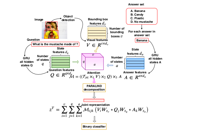
Figure 2: The proposed model when CTI is applied to MC VQA. The details are described in Section 4.1. Best view in color.

4.2 Free-Form Opened-Ended Visual Question Answering

Unlike MC VQA, FFOE VQA treats the answering as a classification problem over the set of predefined answers. Hence the set possible answers for each question-image pair is much more than the case of MC VQA. Therefore the model design proposed in Section 4.1, i.e. for each question-image input, the model takes every possible answers from its answer list to computed the joint representation, causes high computational cost. In addition, the proposed CTI requires all three $V,Q,A$ inputs to compute the joint representation. However, during the testing, there are no available answer information in FFOE VQA. To overcome these challenges, we propose to use Knowledge Distillation [13] to transfer the learned knowledge from a teacher model to a student model. Figure 3 visualizes the proposed design for FFOE VQA.

Our teacher model takes triplets of image-question-right answer as inputs. Each triplet is passed through the proposed CTI to get the joint representation $z$. The joint representation $z$ is then passed through a multiclass classifier (over the set of predefined answers) to get the prediction which is similar to [37]. The Cross Entropy loss is used for training the teacher model. Regarding the student models, any state-of-the-art VQA can be used. In our experiments, we use BAN2 [18] or SAN [43] as student models. The student models take pairs of image-question as inputs and treat the prediction as a mutilclass classification problem. The loss function for the student model is defined as

$$\mathcal{L}_{KD}=\alpha T^{2}\mathcal{L}_{CE}(Q^{\tau}_{S},Q^{\tau}_{T})+(1-\alpha)\mathcal{L}_{CE}(Q_{S},y_{true})$$ (14)

where $\mathcal{L}_{CE}$ stands for Cross Entropy loss; $Q_{S}$ is the standard softmax output of the student; $y_{true}$ is the ground-truth answer labels; $\alpha$ is a hyper-parameter for controlling the importance of each loss component; $Q^{\tau}_{S},Q^{\tau}_{T}$ are the softened outputs of the student and the teacher using the same temperature parameter $T$ [13], which are computed as follows

$$Q^{\tau}_{i}=\frac{exp(l_{i}/T)}{\sum_{i}exp(l_{i}/T)}$$ (15)

where for both teacher and the student models, the logit $l$ is the predictions outputted by the corresponding classifiers.

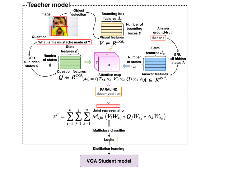
Figure 3: The proposed model when CTI is applied on FFOE VQA. The details are described in Section 4.2. Best view in color.

Following by the current state of the art in FFOE VQA [18], for image representation, we use object detection-based features with FPN detector (ResNet152 backbone)[22], in which the number of maximum detected bounding boxes is set to $50$. For question and answer representations, we trim question and answer to a maximum of 12 words which will then be zero-padded if shorter than 12 words. Each word is then represented by a 600-D vector that is a concatenation of the 300-D GloVe word embedding [32] and the augmenting embedding from training data as [18]. In the other words, a question is with a representation with size $12\times 600$. It is similar for answer.

5 Experiments

5.1 Dataset and evaluation protocol

Dataset. We conduct the experiments on three benchmarking VQA datasets that are Visual7W [47] for the MC VQA, VQA-2.0 [10] and TDIUC [17] for the FFOE VQA. We use training set to train and validation set to evaluate in all mentioned datasets when conducting ablation study.

Implementation details. Our CTI is implemented using PyTorch [31]. The experiments are conducted on a NVIDIA Titan V GPUs with 12GB RAM. In all experiments, the learning rate is set to $10^{-3}$. Batch size is set to $128$ for training MC VQA and $256$ for training FFOE VQA. When training both MC VQA model (Section 4.1) and FFOE VQA model (Section 4.2), except the image representation extraction, other components are trained end-to-end. The temperature parameter $T$ in (15) is set to $3$. The dimension of the joint representation $z$ is set at $1,024$ for both MC VQA and FFOE VQA.

Evaluation Metrics. We follow the literature [3, 17, 47] in which the evaluation metrics for each VQA task are different. For FFOE VQA, the single accuracy, which is a standard VQA accuracy (Acc) [3], is applied for both TDIUC and VQA-2.0 datasets. In addition, due to the imbalance in the question types of TDIUC dataset, follow [17], we also report four other metrics that compensate for the skewed question-type distribution. They are Arithmetic MPT (Ari), Arithmetic Norm-MPT (Ari-N), Harmonic MPT (Har), and Harmonic Norm-MPT (Har-N). For MC VQA, we follow the evaluation metric (Acc-MC) proposed by [47] in which the performance is measured by the portion of correct answers selected by the VQA model from the candidate answer set.

5.2 Ablation study

QT	Models	Evaluation metrics
		Acc	Ari	Har	Ari-N	Har-N
with Abs	BAN2-CTI	87.0	72.5	65.5	45.8	28.6
	BAN2[18]	85.5	67.4	54.9	37.4	15.7
	SAN-CTI	84.5	68.7	59.9	41.3	23.3
	SAN[43]	82.3	65.0	53.7	35.4	14.7
w/o Abs	BAN2-CTI	85.0	70.6	63.8	41.5	26.9
	BAN2[18]	81.9	64.6	52.8	31.9	14.6
	SAN-CTI	82.8	66.7	58.1	36.8	21.8
	SAN[43]	79.1	62.4	51.7	30.2	13.7

Table 1: Overall performance of the proposal and the baselines BAN2, SAN in different evaluation metrics on TDIUC validation set. The performance is shown with and without considering Absurd question category. BAN2-CTI and SAN-CTI are student models trained under our proposed CTI teacher model.

The effectiveness of CTI on FFOE VQA. We compare our distilled BAN2 (BAN2-CTI) and distilled SAN (SAN-CTI) student models to the state-of-the-art baselines BAN2 [18] and SAN [43]. Table 1 presents a comprehensive evaluation on five different metrics on TDIUC. Among all metrics, on overall, our BAN2-CTI and SAN-CTI outperform corresponding baselines by a noticeable margin. These results confirm the effectiveness of our proposed CTI for learning the joint representation. In addition, the proposed teacher model (Figure 3) is also effective. It successfully transfers useful learned knowledge to the student models. Note that in Table 1, the “Absurd” question category indicates the cases in which input questions are irrelevant to the image contents. Thus, the answers are always “does not apply”, i.e., “no answer”. Using these meaningless answers when training the teacher causes negative effect when learning the joint representation, hence, reducing the model capacity. If the “Absurd” category is not taken into account, the proposed model achieves more improvements over baselines.

Question-types	BAN2-CTI	BAN2 [18]	SAN-CTI	SAN [43]
Scene Rec	94.5	93.1	93.6	92.3
Sport Rec	96.3	95.7	95.5	95.5
Color Attr	74.3	67.5	70.9	60.9
Other Attr	60.5	53.2	56.4	46.2
Activity Rec	63.2	54.0	54.5	51.4
Positional Rec	40.5	27.9	34.3	27.9
Sub-Obj Rec	89.3	87.5	87.6	87.5
Absurd	93.9	98.2	90.6	93.4
Util & Aff	36.3	24.0	31.0	26.3
Obj Pres	96.1	95.1	94.9	92.4
Count	59.7	53.9	55.6	52.1
Sentiment	66.1	58.7	59.9	53.6

Table 2: Performance (Acc) of the proposal and the baselines BAN2, SAN for each question-type on TDIUC validation set. BAN2-CTI and SAN-CTI are student models trained under our compact trilinear interaction teacher model.

Table 2 presents detail performances with Acc metric over each question category of TDIUC when all categories, including “Absurd”, are used for training. The results show that we achieve the best results on all question categories but “Absurd”. We note that in the real applications, the “Absurd” question problem may be mitigated in some cases by using a simple trick, i.e., asking a “presence question” before asking the main question, e.g., we have an image with no human but the main question is “Is the people wearing hat?”, i.e., a “Absurd” question. By asking a “presence question” as “Are there any people in the picture?”, we can have a confirmation about the presence of human in the considered image, before asking the main question.

Ref models	Validation Accuracy	Test-dev Accuracy
Bottom-up [37]	63.2	65.4
SAN [43]	61.7	63.0
SAN-CTI	62.1	63.4
BAN2 [18]	65.6	66.5
BAN2-CTI	66.0	67.4

Table 3: Performance of the proposal and baselines BAN2, SAN in VQA-2.0 validation set and test-dev set. BAN2-CTI and SAN-CTI are student models trained under proposed teacher model.

Table 3 presents comparative results between our distilled student models and two baselines BAN2, SAN on Acc metric on VQA-2.0. Although our proposal outperforms the baselines, the improvement gap is not much. This is understandable because the VQA-2.0 dataset has a large number of questions of which answers are “yes/no” or contain only one word (i.e., answers for “number” question types). These answers have little semantic meanings which prevent proposed trilinear interaction from promoting its efficiency.

The effectiveness of CTI on MC VQA. We still use the state-of-the-art BAN2 [18] and SAN [43] as baselines and conduct experiments on Visual7W dataset. In MC VQA, in both training and testing, each image-question pair has a corresponding answer list that contains four answers. To make a fair comparison, we try different pair combinations over three modalities (image, question, and answer) for the baselines BAN2 and SAN. Similar to [41], we find the following combination gives best results for the baselines. Using BAN2 (or SAN), we first compute the joint representation between image and question; and the joint representation between image and answer. Then, we concatenate the two computed representations to get the joint “image-question-answer” representation, and pass it through VQA classifier with cross entropy loss for training the baseline.

Ref models	Visual7W validation set
	Acc-MC	Number of parameters
BAN2 [18]	65.7	$\sim$ 86.5M
SAN [43]	59.3	$\sim$ 69.7M
CTI	67.0	$\sim$ 66.5M

Table 4: The performance (Acc-MC) and the number of parameters of the proposed MC VQA model and the baselines BAN2, SAN on Visual7W validation set.

Table 4 presents comparative results on Visual7W with Acc-MC metric. The results show that our proposed model outperforms the baselines by a noticeable margin. These results confirm that the joint representation learned by the proposed trilinear interaction achieves better performance than the combination of joint representations computed by BAN (or SAN) of pairs of modalities. In addition, in Table 4 we also provide the number of total parameters of our proposed MC VQA model with CTI (Figure 2) and BAN2, SAN. The results show that our model requires less memory than those baselines. That means that the proposed MC VQA model with CTI not only outperforms the baselines in term of accuracy, but also more efficient than those baselines in term of the usage memory. Figure 4 visualizes the attention map resulted by CTI for an example of image-question-answer. The attention map is computed by (12).

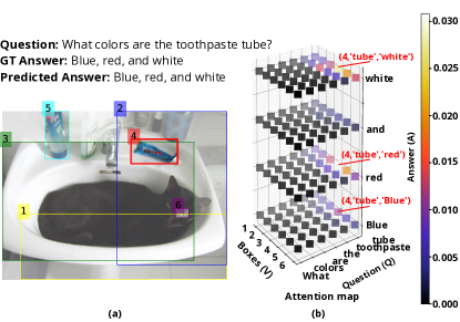
Figure 4: The visualization of an attention map (b) computed from Eq. (12) for an image-question-answer input (a). The attention map indicates attention weights over triplets of “detected bounding box - word in question - word in answer”. The higher weight of a triplet is, the more contribution it makes to the joint representation. We can see that three triplets (V=4, Q=“tube”, A=“white”), (V=4, Q=“tube”, A=“red”), (V=4, Q=“tube”, A=“blue”) have high weight values. That means that these triplets give high contribution to the joint representation. The input sample (a) is from Visual7W validation set. Best view in color.

5.3 Comparison with the state of the art

To further evaluate the effectiveness of CTI, we conduct a detailed comparison with the current state of the art. For FFOE VQA, we compare our proposal with the recent state-of-the-art methods on TDIUC and VQA-2.0 datasets, including SAN [43], QTA [35], BAN2 [18], Bottom-up [37], MCB [8], and RAU [29]. For MC VQA, we compare with the state-of-the-art methods on Visual7W dataset, including BAN2 [18], SAN [43], MLP [16], MCB [8], STL [41], and fPMC [14]). It is worth noting that depending on tasks FFOE VQA or MC VQA, we use different representations for images and questions as clearly mentioned in Section 4. This ensures a fair comparison with compared methods.

Models	Evaluation metrics
	Acc	Ari	Har	Ari-N	Har-N
BAN2 [18]	85.5	67.4	54.9	37.4	15.7
SAN [43]	82.3	65.0	53.7	35.4	14.7
QTA [35]	85.0	69.1	60.1	_	_
MCB [8]	79.2	65.8	58.0	39.8	24.8
RAU [29]	84.3	67.8	59.0	41.0	24.0
SAN-CTI	84.5	68.7	59.9	41.3	23.3
BAN2-CTI	87.0	72.5	65.5	45.8	28.6

Table 5: Performance comparison between different approaches with different evaluation metrics on TDIUC validation set. BAN2-CTI and SAN-CTI are the student models trained under our compact trilinear interaction teacher model.

Regarding FFOE VQA, Tables 3 and 5 show comparative results on VQA-2.0 and TDIUC respectively. Specifcaly, Table 5 shows that our distilled student BAN2-CTI outperforms all compared methods over all metrics by a large margin, i.e., our model outperforms the current state-of-the-art QTA [35] on TDIUC by $3.4\%$ and $5.4\%$ on Ari and Har metrics, respectively. The results confirm that the proposed trilinear interaction has learned informative representations from the three inputs and the learned information is effectively transferred to student models by distillation.

Dataset	Ref models	Acc-MC
Visual7W test set	MLP [16]	67.1
	MCB [8]	62.2
	fPMC [14]	66.0
	STL [41]	68.2
	SAN [43]	61.5
	BAN2 [18]	67.5
	CTI	69.3
	CTIwBoxes	72.3

Table 6: Performance comparison between different approaches on Visual7W test set. Both training set and validation set are used for training. All models but CTIwBoxes are trained with same image and question representations. Both train set and validation set are used for training. Note that CTIwBoxes is the proposed CTI model using Bottom-up features [2] instead of grid features for image representation.

Regarding MC VQA, Table 6 shows that the proposed model (denoted as CTI in Table 6) outperforms compared methods by a noticeable margin. Our model outperforms the current state-of-the-art STL [41] $1.1\%$. Again, this validates the effectiveness of the proposed joint presentation learning, which precisely and simultaneously learns interactions between the three inputs. We note that when comparing with other methods on Visual7W, for image representations, we used the grid features extracted from ResNet-512 [12] for a fair comparison. Our proposed model can achieve further improvements by using the object detection-based features used in FFOE VQA. With new features, our model denoted as CTIwBoxes in Table 6 achieve $72.3\%$ accuracy with Acc-MC metric which improves over the current state-of-the-art STL [41] $4.1\%$.

5.4 Further analysis

The effectiveness of PARALIND decomposition. In this section, we compute the decomposition rate of PARALIND. For a fully interaction between the three inputs, using (1), we would need to learn $2199.02$ billions parameters which is infeasible in practice. By using the PARALIND decomposition presented in Section 3 with the provided settings, i.e., the number of slicing $R=32$ and the dimension of the joint representation $d_{z}=1024$, the number of parameters that need to learn is only $33.69$ millions. In the other words, we achieve a decomposition rate $\approx 65,280$.

Compact Trilinear Interaction as the generalization of BAN [18]. The proposed compact trilinear interaction model can be seen as a generalization of the state-of-the-art joint embedding BAN [18].

In BAN, each input contains an image representation $V$ $\in\mathds{R}^{d_{v}\times v}$ and a question representation $Q\in\mathds{R}^{d_{q}\times q}$. The trilinear interaction model can be modified to adapt to these two inputs. The joint representation $z\in\mathds{R}^{d_{z}}$ in (1) can be adapted for two input as

$$z^{T}=\left(\mathcal{T}_{vq}\times_{1}vec(V)\right)\times_{2}vec(Q)$$ (16)

where $\mathcal{T}_{vq}\in\mathds{R}^{d_{V}\times d_{Q}\times d_{z}}$ is a learnable tensor; $vec(V)$ is the vectorization of $V$ and $vec(Q)$ is the vectorization of $Q$ which output row vectors; $d_{V}=d_{v}\times v$; $d_{Q}=d_{q}\times q$.

By applying “Parameter factorization” described in Section 3.2, $z$ in (16) can be approximated based on (13) as

$$z^{T}=\sum_{i=1}^{v}\sum_{j=1}^{q}\mathcal{M}_{ij}\left(V_{i}^{T}W_{z_{v}}\circ Q_{j}^{T}W_{z_{q}}\right)$$ (17)

where $W_{z_{v}}\in\mathds{R}^{d_{v}\times d_{z}}$ and $W_{z_{q}}\in\mathds{R}^{d_{q}\times d_{z}}$ are learnable factor matrices; $\mathcal{M}_{ij}$ is an attention weight of attention map $\mathcal{M}\in\mathds{R}^{v\times q}$ which can be computed from (12) as

$$\mathcal{M}=\sum^{R}_{r=1}{\llbracket\mathcal{G}_{r};V^{T}W_{v_{r}},Q^{T}W_{q_{r}}\rrbracket}$$ (18)

where $W_{v_{r}}\in\mathds{R}^{d_{v}\times d_{v_{r}}}$ and $W_{q_{r}}\in\mathds{R}^{d_{q}\times d_{q_{r}}}$ are learnable factor matrices; $d_{v_{r}}=d_{v}/R$; $d_{q_{r}}=d_{q}/R$; each $\mathcal{G}_{r}\in\mathds{R}^{d_{v_{r}}\times d_{q_{r}}}$ is a learnable Tucker tensor.

Interestingly, (17) can be reorganized to have a form of BAN [18] as

$$z_{k}=\sum_{i=1}^{v}\sum_{j=1}^{q}\mathcal{M}_{ij}\left(V_{i}^{T}\left(W_{{z_{v}}_{k}}W_{{z_{q}}_{k}}^{T}\right)Q_{j}\right)$$ (19)

where $z_{k}$ is the $k^{th}$ element of the joint representation $z$; $W_{{z_{v}}_{k}}$ and $W_{{z_{q}}_{k}}$ are $k^{th}$ column in factor matrices $W_{z_{v}}$ and $W_{z_{q}}$. Note that in (19), our attention map $\mathcal{M}$ is resulted from the PARALIND decomposition, while in BAN [18], their attention map is computed by bilinear pooling.

6 Conclusion

We propose a novel compact trilinear interaction which simultaneously learns high level associations between image, question, and answer in both MC VQA and FFOE VQA. In addition, knowledge distillation is the first time applied to FFOE VQA to overcome the computational complexity and memory issue of the interaction. The extensive experimental results show that the proposed models achieve the state-of-the-art results on three benchmarking datasets.

References

- [1] Devi Parikh Aishwarya Agrawal, Dhruv Batra and Aniruddha Kembhavi. Don’t just assume; look and answer: Overcoming priors for visual question answering. In CVPR, 2018.
- [2] Peter Anderson, Xiaodong He, Chris Buehler, Damien Teney, Mark Johnson, Stephen Gould, and Lei Zhang. Bottom-up and top-down attention for image captioning and VQA. In CVPR, 2018.
- [3] Stanislaw Antol, Aishwarya Agrawal, Jiasen Lu, Margaret Mitchell, Dhruv Batra, C. Lawrence Zitnick, and Devi Parikh. VQA: Visual Question Answering. In ICCV, 2015.
- [4] Jimmy Ba and Rich Caruana. Do deep nets really need to be deep? In NIPS, 2014.
- [5] Hedi Ben-younes, Rémi Cadène, Matthieu Cord, and Nicolas Thome. Mutan: Multimodal tucker fusion for visual question answering. In ICCV, 2017.
- [6] Rasmus Bro, Richard A Harshman, Nicholas D Sidiropoulos, and Margaret E Lundy. Modeling multi-way data with linearly dependent loadings. Journal of Chemometrics: A Journal of the Chemometrics Society, pages 324–340, 2009.
- [7] Guobin Chen, Wongun Choi, Xiang Yu, Tony Han, and Manmohan Chandraker. Learning efficient object detection models with knowledge distillation. In NIPS, 2017.
- [8] Akira Fukui, Dong Huk Park, Daylen Yang, Anna Rohrbach, Trevor Darrell, and Marcus Rohrbach. Multimodal compact bilinear pooling for visual question answering and visual grounding. In EMNLP, 2016.
- [9] Chuang Gan, Yandong Li, Haoxiang Li, Chen Sun, and Boqing Gong. Vqs: Linking segmentations to questions and answers for supervised attention in vqa and question-focused semantic segmentation. In ICCV, 2017.
- [10] Yash Goyal, Tejas Khot, Douglas Summers-Stay, Dhruv Batra, and Devi Parikh. Making the V in VQA matter: Elevating the role of image understanding in visual question answering. In CVPR, 2017.
- [11] Saurabh Gupta, Judy Hoffman, and Jitendra Malik. Cross modal distillation for supervision transfer. In CVPR, 2016.
- [12] Kaiming He, Xiangyu Zhang, Shaoqing Ren, and Jian Sun. Deep residual learning for image recognition. In CVPR, 2016.
- [13] Geoffrey Hinton, Oriol Vinyals, and Jeff Dean. Distilling the knowledge in a neural network. In NIPS Deep Learning Workshop, 2014.
- [14] Hexiang Hu, Wei-Lun Chao, and Fei Sha. Learning answer embeddings for visual question answering. In CVPR, 2018.
- [15] Ilija Ilievski, Shuicheng Yan, and Jiashi Feng. A focused dynamic attention model for visual question answering. arXiv preprint arXiv:1604.01485, 2016.
- [16] Allan Jabri, Armand Joulin, and Laurens Van Der Maaten. Revisiting visual question answering baselines. In ECCV, 2016.
- [17] Kushal Kafle and Christopher Kanan. An analysis of visual question answering algorithms. In ICCV, 2017.
- [18] Jin-Hwa Kim, Jaehyun Jun, and Byoung-Tak Zhang. Bilinear attention networks. In NIPS, 2018.
- [19] Jin-Hwa Kim, Sang-Woo Lee, Donghyun Kwak, Min-Oh Heo, Jeonghee Kim, Jung-Woo Ha, and Byoung-Tak Zhang. Multimodal residual learning for visual qa. In NIPS, 2016.
- [20] Jin-Hwa Kim, Kyoung-Woon On, Woosang Lim, Jeonghee Kim, Jung-Woo Ha, and Byoung-Tak Zhang. Hadamard product for low-rank bilinear pooling. In ICLR, 2017.
- [21] Tamara G Kolda and Brett W Bader. Tensor decompositions and applications. SIAM review, pages 455–500, 2009.
- [22] Tsung-Yi Lin, Piotr Dollár, Ross B. Girshick, Kaiming He, Bharath Hariharan, and Serge J. Belongie. Feature pyramid networks for object detection. In CVPR, 2017.
- [23] Jiasen Lu, Jianwei Yang, Dhruv Batra, and Devi Parikh. Hierarchical question-image co-attention for visual question answering. In NIPS, 2016.
- [24] Chao Ma, Chunhua Shen, Anthony R. Dick, and Anton van den Hengel. Visual question answering with memory-augmented networks. In CVPR, 2018.
- [25] Mateusz Malinowski and Mario Fritz. Towards a visual turing challenge. In NIPS workshop, 2014.
- [26] Mateusz Malinowski, Marcus Rohrbach, and Mario Fritz. Ask your neurons: A neural-based approach to answering questions about images. ICCV, pages 1–9, 2015.
- [27] Hyeonseob Nam, Jung-Woo Ha, and Jeonghee Kim. Dual attention networks for multimodal reasoning and matching. In CVPR, 2017.
- [28] Duy-Kien Nguyen and Takayuki Okatani. Improved fusion of visual and language representations by dense symmetric co-attention for visual question answering. In CVPR, 2018.
- [29] Hyeonwoo Noh and Bohyung Han. Training recurrent answering units with joint loss minimization for vqa. arXiv preprint arXiv:1606.03647, 2016.
- [30] Hyeonwoo Noh, Paul Hongsuck Seo, and Bohyung Han. Image question answering using convolutional neural network with dynamic parameter prediction. In CVPR, 2016.
- [31] Adam Paszke, Sam Gross, Soumith Chintala, Gregory Chanan, Edward Yang, Zachary DeVito, Zeming Lin, Alban Desmaison, Luca Antiga, and Adam Lerer. Automatic differentiation in pytorch. In NIPS 2017 Workshop, 2017.
- [32] Jeffrey Pennington, Richard Socher, and Christopher D. Manning. Glove: Global vectors for word representation. In EMNLP, 2014.
- [33] Adriana Romero, Nicolas Ballas, Samira Ebrahimi Kahou, Antoine Chassang, Carlo Gatta, and Yoshua Bengio. Fitnets: Hints for thin deep nets. In ICLR, 2015.
- [34] Idan Schwartz, Alexander Schwing, and Tamir Hazan. High-order attention models for visual question answering. In NIPS, 2017.
- [35] Yang Shi, Tommaso Furlanello, Sheng Zha, and Animashree Anandkumar. Question type guided attention in visual question answering. In ECCV, 2018.
- [36] Kevin J Shih, Saurabh Singh, and Derek Hoiem. Where to look: Focus regions for visual question answering. In CVPR, 2016.
- [37] Damien Teney, Peter Anderson, Xiaodong He, and Anton van den Hengel. Tips and tricks for visual question answering: Learnings from the 2017 challenge. In CVPR, 2018.
- [38] Damien Teney and Anton van den Hengel. Zero-shot visual question answering. arXiv preprint arXiv:1611.05546, 2016.
- [39] Damien Teney, Lingqiao Liu, and Anton van den Hengel. Graph-structured representations for visual question answering. In CVPR, 2017.
- [40] Damien Teney and Anton van den Hengel. Visual question answering as a meta learning task. In ECCV, 2018.
- [41] Zhe Wang, Xiaoyi Liu, Limin Wang, Yu Qiao, Xiaohui Xie, and Charless Fowlkes. Structured triplet learning with pos-tag guided attention for visual question answering. In WACV, 2018.
- [42] Huijuan Xu and Kate Saenko. Ask, attend and answer: Exploring question-guided spatial attention for visual question answering. In ECCV, 2016.
- [43] Zichao Yang, Xiaodong He, Jianfeng Gao, Li Deng, and Alexander J. Smola. Stacked attention networks for image question answering. In CVPR, 2016.
- [44] Dongfei Yu, Jianlong Fu, Tao Mei, and Yong Rui. Multi-level attention networks for visual question answering. In CVPR, 2017.
- [45] Zhou Yu, Jun Yu, Jianping Fan, and Dacheng Tao. Multi-modal factorized bilinear pooling with co-attention learning for visual question answering. In ICCV, 2017.
- [46] Bolei Zhou, Yuandong Tian, Sainbayar Sukhbaatar, Arthur Szlam, and Rob Fergus. Simple baseline for visual question answering. arXiv preprint arXiv:1512.02167, 2015.
- [47] Yuke Zhu, Oliver Groth, Michael Bernstein, and Li Fei-Fei. Visual7W: Grounded question answering in images. In CVPR, 2016.