A Facet Enumeration Algorithm for Convex Polytopes

Abstract

This paper proposes a novel and simple algorithm of facet enumeration for convex polytopes. The complexity of the algorithm is discussed. The algorithm is implemented in Matlab. Some simple polytopes with known H-representations and V-representations are used as the test examples. Numerical test shows the effectiveness and efficiency of the proposed algorithm. Due to the duality between the vertex enumeration problem and facet enumeration problem, we expect that this method can also be used to solve the vertex enumeration problem.

Keywords: Algorithm, convex polytope, facet enumeration, linear programming.

1 Introduction

For convex polytopes, there are two different but equivalent representations: (a) H-representation, and (b) V-representation. H-representation uses a set of closed half-spaces to define a convex polytope, i.e., a polytope is given as ${\bf A}{\bf x}\leq{\bf b}$, where ${\bf A}\in\mathbb{R}^{m\times d}$ and ${\bf b}\in\mathbb{R}^{m}$ are given, and ${\bf x}\in\mathbb{R}^{d}$ are the set of points in the convex polytope. A $k$-face of a polytope is the set of ${\bf x}$ that meet two conditions: (1) ${\bf A}{\bf x}\leq{\bf b}$, and (2) for some $d-k$ independent rows of ${\bf A}_{k}$, ${\bf A}_{k}{\bf x}={\bf b}$. For $k=0$, a $0$-face of the polytope is a vertex; for $k=1$, a $1$-face of the polytope is an edge; for $k=d-2$, a $(d-2)$-face of the polytope is a ridge; for $k=d-1$, a $(d-1)$-face of the polytope is a facet. In the remainder of the paper, we use vertex, edge, and facet explicitly, but we do not make distinction for other $k$-faces in general. V-representation uses a set of vertices $\mathcal{V}=\{{\bf v}_{1},{\bf v}_{2},\ldots,{\bf v}_{n}\}$ to define a convex polytope as a convex hull of $\mathcal{V}$. Given one of the representations, there is a need, in many applications [1, 7, 9], to know what the other corresponding representation is. The transformation from (a) to (b) is known as the vertex enumeration and the other from (b) to (a) is known as the facet enumeration.

Vertex enumeration is clearly related to the simplex method of linear programming. The so-called double-description method can be dated back to Fourier (1827) [16] and was reinvented by Motzkin [12]. Their method constructs the polytope sequentially by adding one constraint at a time. All new vertices produced must lie on the hyperplanes bounding the constraint currently being inserted. A more popular vertex enumeration method is based on pivoting, which was discussed by Chand and Kapur [6], Dyer [10], Swart [13], among others. The most popular method in this category is the reverse search method proposed by Avis and Fukuda [2]. Their method starts at an “optimum vertex” and traces out a tree in depth order by “reverse” Bland’s rule [4].

Noticing that the dual problem of a vertex (resp. facet) enumeration problem is the facet (resp. vertex) enumeration problem for the same polytope where the input and output are simply interchanged, Bremner, Fukuda and Marzetta [5] pointed out that the vertex enumeration methods can be used for the facet enumeration problem. They suggested using a primal-dual approach proposed in [11] that includes two purely combinatorial algorithms for enumerating all faces of a d-polytope based on the combinatorial vertices’ description and some information on edges. Very recently, Avis and Jordan [3] published a scalable parallel vertex/facet enumeration code. Avis and Jordan’s paper is also a good source to find the related works.

In this paper, we consider the facet enumeration problem for convex polytopes. Given the vertices of a convex polytope, the idea is to first find all edges of the polytope, which provides a vertex/edge diagram that connects any vertex to its neighbor vertices. The information is stored in a matrix ${\bf D}$. For any vertex, using matrix ${\bf D}$, one can create a tree with depth of $d$. If vertices in a path of the tree from root vertex to end vertex form a hyperplane, one can check if all vertices in $\mathcal{V}$ are in the half space defined by the hyperplane. If the answer is true, the hyperplane contains a facet of the polytope, otherwise, it does not. Repeating these steps for all vertices will find all half spaces whose intersection forms the polytope. Using the duality between the vertex enumeration problem and facet enumeration problem, we expect that this method can also be used to solve the vertex enumeration problem with some minor tweaks.

The remainder of the paper is organized as follows: Section 2 provides details of the proposed algorithm. Section 3 discusses the complexity of the algorithm. Section 4 presents some numerical examples to show the effectiveness and efficiency of the algorithm. Concluding remarks are summarized in Section 5.

2 Facet enumeration

Assuming that a d-dimensional polytope has n vertices that are stored in rows in a matrix ${\bf V}$ of dimension of $n\times d$. Each row (vertex) of ${\bf V}$ is denoted by ${\bf v}_{i}$. To have an efficient algorithm, we set the the centroid of the polytope ${\bf v}_{0}$ as the origin which is an interior point of the polytope. This is simply achieved by using

$${\bf u}_{i}={\bf v}_{i}-{\bf v}_{0},\hskip 7.22743pti=1,\ldots,n.$$ (1)

We will denote by $\mathcal{U}=\{{\bf u}_{1},\ldots,{\bf u}_{n}\}$ the set of vertices which form a polytope with its center as the origin of the coordinate system. We also use a matrix

$${\bf U}=\left[\begin{array}[]{c}{\bf u}_{1}\\ \vdots\\ {\bf u}_{n}\end{array}\right]\in\mathbb{R}^{n\times d}$$

to store these vertices. Our idea is to calculate a column vector ${\bf h}_{i}\in\mathbb{R}^{d}$, or the hyperplane ${\bf h}_{i}^{{\rm T}}{\bf x}=1$, where ${\bf x}\in\mathbb{R}^{d}$ is the set of d-dimensional column vectors that spans the hyperplane, so that the $m$ half spaces (associated with the $m$ hyperplanes)

$${\bf H}{\bf x}:=\left[{\bf h}_{1},\ldots,{\bf h}_{m}\right]^{{\rm T}}{\bf x}\leq{\bf e}$$ (2)

defines the polytope.

The algorithm first establishes a vertex/edge diagram that describes all vertex/edge relations of a given polytope. The process is as follows: given any vertex ${\bf u}_{i}$ on the polytope, the proposed algorithm identifies its neighbor vertices which are connected by edges. Let ${\bf u}_{i}$ and ${\bf u}_{j}$ be two vertices of the polytope. The line pass both ${\bf u}_{i}$ and ${\bf u}_{j}$ can be defined by

$$\mathcal{L}=\{{\bf u}_{i}+t({\bf u}_{j}-{\bf u}_{i})~{}|~{}t\in\mathbb{R}\}.$$ (3)

Assuming that a point ${\bf z}$ is on the line of $\mathcal{L}$ and the row vector ${\bf z}-{\bf 0}={\bf z}$ (where ${\bf 0}$ is the origin and the center of the polytope) is perpendicular to the line $\mathcal{L}$, then ${\bf z}$ satisfies the following equations:

$${\bf z}={\bf u}_{i}+t({\bf u}_{j}-{\bf u}_{i}),\hskip 7.22743pt\langle{\bf z},{\bf u}_{j}-{\bf u}_{i}\rangle=0.$$ (4)

Solving (4) for $t$ yields

$$t=-\frac{{\bf u}_{i}({\bf u}_{j}-{\bf u}_{i})^{{\rm T}}}{\|({\bf u}_{j}-{\bf u}_{i})\|^{2}},$$ (5)

which gives

$${\bf z}={\bf u}_{i}-\frac{{\bf u}_{i}({\bf u}_{j}-{\bf u}_{i})^{{\rm T}}}{\|({\bf u}_{j}-{\bf u}_{i})\|^{2}}({\bf u}_{j}-{\bf u}_{i}).$$ (6)

We have the following claim:

Lemma 2.1

${\bf z}\neq{\bf 0}$ if $\mathcal{L}$ does not cross the centroid (origin).

• Since ${\bf z}$ is on $\mathcal{L}$ and $\mathcal{L}$ does not cross ${\bf 0}$, it must have ${\bf z}\neq{\bf 0}$.       

Thus, ${\bf z}={\bf 0}$ implies that ${\bf u}_{j}$ is not a neighbor vertex of ${\bf u}_{i}$ (this will reduce the computational effort if such a scenario appears). Therefore, we may assume, without loss of generality, that ${\bf z}\neq{\bf 0}$. Denote a row vector ${\bf a}={\bf z}/\|{\bf z}\|\neq{\bf 0}$ and a constant $c={\bf a}{\bf z}^{{\rm T}}=\frac{{\bf z}{\bf z}^{{\rm T}}}{\|{\bf z}\|}=\|{\bf z}\|\neq 0$. Then, a hyperplane $\mathcal{P}$ passing line $\mathcal{L}$ with the normal direction ${\bf a}^{{\rm T}}$ is given by

$${\bf a}({\bf x}-{\bf z}^{{\rm T}})={\bf a}{\bf x}-c=0,$$ (7)

where ${\bf a}$ is a known row vector, $c$ is a constant, and ${\bf x}\in\mathbb{R}^{d}$ is any point on the hyperplane $\mathcal{P}$. Dividing both sides by $c$ and denote ${\bf h}^{{\rm T}}={\bf a}/c$, i.e., ${\bf h}$ is a column vector, we get

$${\bf h}^{{\rm T}}{\bf x}=1.$$ (8)

Intuitively, from the construction of $\mathcal{P}$, if for all ${\bf u}_{k}$, we have

$${\bf h}^{{\rm T}}{\bf u}_{k}^{{\rm T}}\leq 1$$ (9)

with equality hold for only ${\bf u}_{i}$ and ${\bf u}_{j}$, then the segment between ${\bf u}_{i}$ and ${\bf u}_{j}$ is an edge of the polytope and ${\bf u}_{i}$ and ${\bf u}_{j}$ are adjacent vertices. We summarize the discussion as the following theorem.

Theorem 2.1

Let ${\bf u}_{i}$ and ${\bf u}_{j}$ be two vertices of a convex polytope. Let $\mathcal{L}$ be the line as defined in (3). For $t$ given in (5), ${\bf z}={\bf u}_{i}+t({\bf u}_{j}-{\bf u}_{i})$ is perpendicular $\mathcal{L}$. Denote ${\bf a}={\bf z}/\|{\bf z}\|$ and $c={\bf a}{\bf z}^{{\rm T}}$ (${\bf a}$ and ${\bf z}$ are row vectors). Let ${\bf h}^{{\rm T}}={\bf a}/c$. Then,

$${\bf h}^{{\rm T}}{\bf x}=1,\hskip 7.22743pt\forall{\bf x}\in\mathbb{R}^{d}$$ (10)

is a hyperplane passing ${\bf u}_{i}$ and ${\bf u}_{j}$, and the following claims hold:

(a) If for all ${\bf u}_{k}$, inequality (9) holds and the equality holds for only ${\bf u}_{i}$ and ${\bf u}_{j}$, then the segment between ${\bf u}_{i}$ and ${\bf u}_{j}$ is an edge of the polytope, i.e., ${\bf u}_{i}$ and ${\bf u}_{j}$ are adjacent vertices.

(b) If for all ${\bf u}_{k}$, inequality (9) holds and the equality holds for more than two but less than $d$ vertices, then the line segment between ${\bf u}_{i}$ and ${\bf u}_{j}$ is on a $k$-face which is part of the hyperplane.

(c) If for all ${\bf u}_{k}$, inequality (9) holds and the equality holds for at least $d$ vertices, then the line segment between ${\bf u}_{i}$ and ${\bf u}_{j}$ is on the hyperplane and a facet of the polytope is part of the hyperplane.

• We show part (a) only because parts (b) and (c) follows similar argument. Since (9) holds for all vertices $k=1,\ldots,n$, all points of the polytope are inside of the half space ${\bf h}^{{\rm T}}{\bf x}\leq 1$. The half space contains the polytope. Since ${\bf u}_{i}$ and ${\bf u}_{j}$ are on the hyperplane, all points on the line segment between ${\bf u}_{i}$ and ${\bf u}_{j}$ are on the hyperplane. Since ${\bf h}^{{\rm T}}{\bf u}_{k}^{{\rm T}}<0$ holds for all ${\bf u}_{k}$ satisfying ${\bf u}_{i}\neq{\bf u}_{k}\neq{\bf u}_{j}$, for any point in the convex hull such that

  $$\sum_{k=1}^{n}\lambda_{k}{\bf u}_{k}$$

  with at least one $\lambda_{k}>0$ and $k\notin\{i,j\}$, we have ${\bf h}^{{\rm T}}\sum_{k=1}^{n}\lambda_{k}{\bf u}_{k}^{{\rm T}}<1$ because $\sum_{k=1}^{n}\lambda_{k}=1$. Therefore, all those points in the convex polytope are not on the hyperplane. Since for all points of the polytope, only line segment between ${\bf u}_{i}$ and ${\bf u}_{j}$ are on the hyperplane, the line segment between ${\bf u}_{i}$ and ${\bf u}_{j}$ is an edge of the polytope.       

Remark 2.1

For the purpose of facet enumeration, we are only interested in cases (a) and (c) because case (a) of Theorem 2.1 implies that ${\bf u}_{j}$ is a neighbor vertex of ${\bf u}_{i}$, which is used to construct vertex/edge diagram, and case (c) will be recorded to reduce computational effort.

If for at least one of ${\bf u}_{k}$, $k=1,\ldots,n$, inequality (9) does not hold, then we need to be a little bit more careful. Note that the middle point between ${\bf u}_{j}$ and ${\bf u}_{i}$ is $\frac{{\bf u}_{j}+{\bf u}_{i}}{2}$, which is also the vector from the origin to the middle point of ${\bf u}_{j}$ and ${\bf u}_{i}$. Therefore, for a row vector

$${\bf y}\neq\frac{{\bf u}_{j}+{\bf u}_{i}}{2},$$ (11)

then, ${\bf y}-\frac{{\bf u}_{j}+{\bf u}_{i}}{2}$ is a vector from the middle point of ${\bf u}_{j}$ and ${\bf u}_{i}$ pointing to ${\bf y}$. We consider all ${\bf y}$ such that ${\bf y}-\frac{{\bf u}_{j}+{\bf u}_{i}}{2}$ is perpendicular to ${{\bf u}_{j}-{\bf u}_{i}}$. Clearly, ${\bf y}$ must satisfy

$$\Biggl{\langle}{\bf y}-\frac{{\bf u}_{j}+{\bf u}_{i}}{2},~{}~{}{\bf u}_{j}-{\bf u}_{i}\Biggr{\rangle}=0,$$ (12)

where $\langle\cdot,\cdot\rangle$ denotes the inner product of its arguments. This is equivalent to

$${\bf y}({\bf u}_{j}-{\bf u}_{i})^{{\rm T}}=\frac{1}{2}({\bf u}_{j}+{\bf u}_{i})({\bf u}_{j}-{\bf u}_{i})^{{\rm T}}.$$ (13)

We want to find a bounded vector ${\bf y}-\frac{{\bf u}_{j}+{\bf u}_{i}}{2}$ such that the smallest angle between ${\bf y}-\frac{{\bf u}_{j}+{\bf u}_{i}}{2}$ and ${\bf u}_{k}-\frac{{\bf u}_{j}+{\bf u}_{i}}{2}$, for $k\notin\{i,j\}$, is maximized, which is equivalent to solving the following mini-max problem:

$$\min_{{\bf y}}\max_{k\notin\{i,j\}}\Bigl{\langle}\frac{{\bf y}-\frac{{\bf u}_{j}+{\bf u}_{i}}{2}}{\|{\bf y}-\frac{{\bf u}_{j}+{\bf u}_{i}}{2}\|},\frac{{\bf u}_{k}-\frac{{\bf u}_{j}+{\bf u}_{i}}{2}}{\|{\bf u}_{k}-\frac{{\bf u}_{j}+{\bf u}_{i}}{2}\|}\Bigr{\rangle}.$$ (14)

However, in stead of considering the nonlinear problem (14), we prefer to deal with a simpler problem. Let

$$f=\max_{k\notin\{i,j\}}\Bigl{\langle}{\bf y}-\frac{{\bf u}_{j}+{\bf u}_{i}}{2},{\bf u}_{k}-\frac{{\bf u}_{j}+{\bf u}_{i}}{2}\Bigr{\rangle}.$$ (15)

We consider the following linear programming problem:

$$\min_{{\bf y},f} ~{}~{}~{}f$$ (16a)

$$s.t. ~{}~{}~{}({\bf y}-\frac{{\bf u}_{j}+{\bf u}_{i}}{2})({\bf u}_{k}-\frac{{\bf u}_{j}+{\bf u}_{i}}{2})^{{\rm T}}\leq f,~{}~{}~{}~{}k\notin\{i,j\},$$ (16b)

$$~{}~{}~{}{\bf y}({\bf u}_{j}-{\bf u}_{i})^{{\rm T}}=\frac{1}{2}({\bf u}_{j}+{\bf u}_{i})({\bf u}_{j}-{\bf u}_{i})^{{\rm T}},$$ (16c)

$$~{}~{}-{\bf 1}\leq{\bf y}-\frac{{\bf u}_{j}+{\bf u}_{i}}{2}\leq{\bf 1},$$ (16d)

where ${\bf 1}$ is a row vector of all ones. There are many efficient algorithms [8, 14, 15] for solving the LP problem, which is out of the scope of our discussion here. Let ${\bf y}^{*}$ and $f^{*}$ be the solution of (16) (${\bf y}^{*}$ is a constant row vector), then the column vector ${\bf x}$ in the following equation

$$\left({\bf y}^{*}-\frac{{\bf u}_{j}+{\bf u}_{i}}{2}\right)\left({\bf x}-(\frac{{\bf u}_{j}+{\bf u}_{i}}{2})^{{\rm T}}\right)=0$$ (17)

defines a plane that is perpendicular to ${\bf y}^{*}-\frac{{\bf u}_{j}+{\bf u}_{i}}{2}$ and passes the line segment between ${\bf u}_{i}$ and ${\bf u}_{j}$. Substituting ${\bf x}^{{\rm T}}={\bf u}_{i}$ to the left side of (17) and applying (12) gives

$$-\frac{1}{2}\Biggl{\langle}{\bf y}^{*}-\frac{{\bf u}_{j}+{\bf u}_{i}}{2},~{}~{}{\bf u}_{j}-{\bf u}_{i}\Biggr{\rangle}=0.$$ (18)

Therefore, ${\bf u}_{i}$ is on the plane defined by (17). Substituting ${\bf x}^{{\rm T}}={\bf u}_{j}$ to the left side of (17) and applying (12) gives

$$\frac{1}{2}\Biggl{\langle}{\bf y}^{*}-\frac{{\bf u}_{j}+{\bf u}_{i}}{2},~{}~{}{\bf u}_{j}-{\bf u}_{i}\Biggr{\rangle}=0.$$ (19)

Therefore, ${\bf u}_{j}$ is on the plane defined by (17). Let ${\bf h}^{{\rm T}}={\bf y}^{*}-\frac{{\bf u}_{j}+{\bf u}_{i}}{2}$, according to (11), ${\bf h}\neq{\bf 0}$. Assuming that the middle point of ${\bf u}_{i}$ and ${\bf u}_{j}$ is not in the origin, i.e., $\frac{{\bf u}_{j}+{\bf u}_{i}}{2}\neq{\bf 0}$, we can write the plane of (17) as

$${\bf h}^{{\rm T}}{\bf x}={\bf h}^{{\rm T}}\left(\frac{{\bf u}_{j}+{\bf u}_{i}}{2}\right)^{{\rm T}}=c\neq 0.$$ (20)

If the minimum of (16) $f^{*}<{\bf h}^{{\rm T}}\left(\frac{{\bf u}_{j}+{\bf u}_{i}}{2}\right)^{{\rm T}}$, it means that all ${\bf u}_{k}$, $k\notin\{i,j\}$, are not on the plane, and they are all on one side of the plane, therefore, the line segment connecting ${\bf u}_{j}$ and ${\bf u}_{i}$ is an edge of the polytope. If $f^{*}={\bf h}^{{\rm T}}\left(\frac{{\bf u}_{j}+{\bf u}_{i}}{2}\right)^{{\rm T}}$, it means that besides ${\bf u}_{j}$ and ${\bf u}_{i}$, there are additional vertices ${\bf u}_{k}$, $k\notin\{i,j\}$ on the plane. Although all vertices are on the same side of the plane defined by (17), ${\bf u}_{j}$ and ${\bf u}_{i}$ do not form an edge of the polytope. If $f^{*}>{\bf h}^{{\rm T}}\left(\frac{{\bf u}_{j}+{\bf u}_{i}}{2}\right)^{{\rm T}}$, it means that it is impossible to find a plane which passes ${\bf u}_{j}$ and ${\bf u}_{i}$, such that all ${\bf u}_{k}$ are on the same side of the plane. Therefore, ${\bf u}_{j}$ and ${\bf u}_{i}$ does not form an edge of the polytope.

Summarizing the discussion above, we have the following theorem.

Theorem 2.2

Let ${\bf u}_{i}$ and ${\bf u}_{j}$ be any two vertices of a convex polytope, ${\bf y}^{*}$ and $f^{*}$ be the optimal solution of (16). Denote that $c={\bf h}^{{\rm T}}\left(\frac{{\bf u}_{j}+{\bf u}_{i}}{2}\right)^{{\rm T}}$, then the following claims hold:

(a) If $f^{*}<c$, then, the line segment connecting ${\bf u}_{j}$ and ${\bf u}_{i}$ is an edge of the polytope.

(b) If $f^{*}=c$, then, ${\bf u}_{j}$ and ${\bf u}_{i}$ do not form an edge of the polytope and the hyperplane contains either a $k$-face if less than $d$ vertices are on the hyperplane or a facet if at least $d$ vertices are on the hyperplane.

(c) If $f^{*}>c$, then, ${\bf u}_{j}$ and ${\bf u}_{i}$ does not form an edge of the polytope and the hyperplane does not form a $k$-face or a facet of the polytope.

Remark 2.2

Although Theorem 2.2 gives a clear criterion to determine if two vertices form an edge of a polytope, Theorem 2.1 needs significantly less computation in general. To have an efficient facet enumeration algorithm, Theorem 2.2 should be used only if Theorem 2.1 cannot determine if two vertices form an edge of a polytope.

Now we discuss the information storage, which is also important for the algorithm design. Let ${\bf D}$ be the $n\times n$ adjacency matrix whose $(i,j)$ element is one if the line segment between ${\bf u}_{i}$ and ${\bf u}_{j}$ is an edge or is zero otherwise. Matrix ${\bf D}$ is obtained by the process described in Theorems 2.1 and 2.2. Since ${\bf D}$ is symmetric, using this property will reduce the computational effort to find all edges of the polytope. We also use a matrix ${\bf F}=(f_{i,j})$, whose rows represent facets and columns represent vertices, such that $f_{i,j}=1$ if vertex $j$ is on the $i$th facet or $f_{i,j}=0$ otherwise. If a facet is found in the process described in Theorem 2.1, i.e., inequality (9) holds for all vertices and equality holds for at least $d$ vertices, a complete row of ${\bf F}$ can be obtained by checking the vertices using (9).

The proposed algorithm has two loops. The outer loop uses breadth-first search. Starting from vertex ${\bf u}_{1}$, the root of the tree, the algorithm finds all facets that intersect at ${\bf u}_{1}$; this brings in new vertices on each of these facets, for each of these new vertices entered in current iteration, the algorithm finds all facets that intersect at the new vertex; the process is repeated until facets for all $n$ vertices are found. To efficiently carry out the iteration, we denote by $\mathcal{U}_{o}$ the set of vertices for which all relevant facets have been found, by $\mathcal{U}_{c}$ the set of vertices in the current iteration for which the associated hyperplanes are to be determined, by $\mathcal{U}_{t}$ the set of the vertices that are not in $\mathcal{U}_{c}$ yet and therefore whose facets have not been examined. The process will terminate when $\mathcal{U}_{o}$ includes all vertices of $\{{\bf u}_{1},\ldots,{\bf u}_{n}\}$.

Having the vertix/edge diagram of ${\bf D}$ that connects all the vertices in $\mathcal{V}$, we use the following method to identify all the facets of the polytope. First, assuming $\mathcal{U}_{o}=\emptyset$ at the beginning, we create a tree starting from the first vertex ${\bf u}_{1}\in\mathcal{U}_{c}$. For ${\bf u}_{i}\in\mathcal{U}_{c}$, we want to find all facets that intersect at ${\bf u}_{i}$. Since each of the facets that passes ${\bf u}_{i}$ can be associated to an edge, for each of these edges directly connected to ${\bf u}_{i}$, we can create a sub-tree of length $d$ as follows. The nonzero $(i,j)$ elements of the adjacency matrix ${\bf D}$ define the tree under the vertex ${\bf u}_{i}$. For each ${\bf u}_{i}$, assuming that ${\bf u}_{i}$ is the $i$th vertex, we look at the $i$th row of ${\bf D}$ to select the next vertex $j$ among all $(i,j)=1$ such that the $j$th vertex has not been used in the construction of existing hyperplanes; once vertex $j$ is selected, we look at the $j$th row of ${\bf D}$ to select the next vertex $k$ among all $(j,k)=1$ such that the $k$th vertex has not been used in the construction of existing facets; repeat this step until $d$ vertices are found.

Since hyperplane (10) is uniquely defined by ${\bf h}$, we will loosely use ${\bf h}_{i}\in\mathbb{R}^{d}$ for the $i$th facet of the polytope if the hyperplane ${\bf h}_{i}$ contains a facet. Let ${\bf u}_{i_{1}}$ be one of vertices in the vertex set $\mathcal{U}_{c}$ in current iteration. We say that $\{{\bf u}_{i_{1}},{\bf u}_{i_{2}},\ldots,{\bf u}_{i_{d}}\}$ is a branch of the tree under ${\bf u}_{i_{1}}$ if for $i_{j}\in\{i_{2},\ldots,i_{d-1}\}$, ${\bf u}_{i_{j}}$ is connected to only ${\bf u}_{i_{j-1}}$ and ${\bf u}_{i_{j+1}}$ in the set of $\{{\bf u}_{i_{1}},{\bf u}_{i_{2}},\ldots,{\bf u}_{i_{d}}\}$. Given these $d$ vertices $\{{\bf u}_{i_{1}},\ldots,{\bf u}_{i_{d}}\}$ which is on the branch of the tree starting from ${\bf u}_{i_{1}}$, one can solve the linear system

$$\left[\begin{array}[]{c}{\bf u}_{i_{1}}\\ \vdots\\ {\bf u}_{i_{d}}\end{array}\right]{\bf h}_{i}:={\bf U}_{i}{\bf h}_{i}={\bf e}.$$ (21)

for the candidate facet ${\bf h}_{i}$. If ${\bf h}_{i}^{{\rm T}}{\bf u}_{k}^{{\rm T}}\leq 1$ for $k=1,\ldots,n$, then ${\bf h}_{i}$ is the hyperplane that includes the $i$th facet. Since (21) may also create an unwanted hyperplane, these unwanted hyperplanes can be identified using one of the following rules: first, inequality ${\bf h}_{i}^{{\rm T}}{\bf u}_{i}^{{\rm T}}\leq 1$ is violated, i.e.,

$${\bf U}{\bf h}_{i}\leq{\bf e}$$ (22)

does not hold for some ${\bf u}_{i}\in{\bf U}$; second, the hyperplane has been found earlier in this process (in this case, the hyperplane will not be add to the matrix ${\bf H}$); third, $\langle{\bf u}_{i},{\bf h}_{i}\rangle<0$. If the newly found hyperplane contains a facet of the convex polytope that is not in the matrix ${\bf H}$, it is then added to ${\bf H}$ and matrix ${\bf F}$ is updated accordingly. Otherwise, discard the hyperplane and continue the search in the tree.

For ${\bf u}_{i}\in\mathcal{U}_{c}$, the idea of the proposed algorithm is to examine all branches ${\bf u}_{i_{1}},\ldots,{\bf u}_{i_{d}}$ under ${\bf u}_{i}={\bf u}_{i_{1}}\in\mathcal{U}_{c}$ in a systematically method to reduce the effort to find facets associated with ${\bf u}_{i}$ that has not been found.

However, given the vertex ${\bf u}_{i}\in\mathcal{U}_{c}$, we may not need to calculate all hyperplanes associated with it because some facets associated with ${\bf u}_{i}$ may be on other hyperplanes defined by some ${\bf h}_{j}$ which have been found in current or previous iterations. A check as indicated early using matrix of ${\bf F}$ may significantly reduce the amount of calculation. We may even terminate early if the checking finds that for every vertex ${\bf u}_{i}\in\mathcal{U}_{t}$, all its associated hyperplanes have been found before the current iteration.

Denote the number of members of a set $\mathcal{U}$ by $|\mathcal{U}|$. The proposed algorithm is therefore given as follows:

Algorithm 2.1

Data: Vertex matrix ${\bf V}$.  
Initial step: Calculate centroid ${\bf v}_{0}$ and vertex set $\mathcal{U}$, adjacent matrix ${\bf D}$, and initial facet/vertex matrix ${\bf F}$. Set up initial $\mathcal{U}_{0}$, $\mathcal{U}_{c}$, and $\mathcal{U}_{t}$.

• While $|\mathcal{U}_{0}|<n$

  • For $i=1$: $|\mathcal{U}_{c}|$

    • Step 1: Using ${\bf F}$ to determine $k_{f}$, the number of facets that include ${\bf u}_{i}$ among all facets that has been found so far. Denote the set of these facets by $\mathcal{F}_{i}:=\{j~{}|~{}F_{j,i}=1~{}\}$.

    • Step 2: Using ${\bf D}$ to determine $k_{e}$, the number of edges that are connected to ${\bf u}_{i}$. Denote the set of these edges by $\mathcal{D}_{i}:=\{j~{}|~{}D_{i,j}=1~{}\}$.

    • Step 3: For $i_{k}\in\mathcal{D}_{i}\setminus\mathcal{F}_{i}$ ($i_{k}=1:k_{e}-k_{f}$)

      • Step a: Search a branch of the tree under ${\bf u}_{i}$ to determine

        $${\bf S}_{i}:=\{{\bf u}_{i_{k}}~{}|~{}\mbox{${\bf u}_{i_{k}}$ form a branch of the tree under ${\bf u}_{i}$}\}.$$ (23)

      • Step b: Compute the directional vectors ${\bf h}_{i}$ using (21).

      • Step c: If ${\bf h}_{i}^{{\rm T}}$ is not a row of ${\bf H}$, in addition, equation (22) hold, and moreover $\langle{\bf u}_{i},{\bf h}_{i}\rangle>0$, save ${\bf h}_{i}^{{\rm T}}$ in ${\bf H}$ and update ${\bf F}$. Otherwise, continue the search using the next edge in $\mathcal{D}_{i}\setminus\mathcal{F}_{i}$ by repeat Step a.

    • end (for $i_{k}$ loop)

    • Step 4: Update $\mathcal{U}_{o}=\mathcal{U}_{o}\cup\mathcal{U}_{c}$, create new $\mathcal{U}_{c}$ with vertices newly entered in the above loop, and remove those vertices from $\mathcal{U}_{t}$.

  • end (for $i$ loop)

• end (while loop)

Recover the polytope by shifting the origin ${\bf H}({\bf x}-{\bf v}_{0})\leq{\bf e}.$

Remark 2.3

The algorithm can easily be modified for parallel implementation.

3 Complexity analysis

The complexity of the algorithm is analyzed in this section. First, to obtain the information of the ${\bf D}$ matrix, one needs to examine

$$(n-1)+(n-2)+\cdots+1=\frac{n(n+1)}{2}$$

pairs of vertices of the polytope. If all vertices can be identified by Theorem 2.1, then for each pair of vertices, the calculation of $t$ using (5) requires $4d$ flops; given ${\bf u}_{j}-{\bf u}_{i}$ which is obtained in the calculation of $t$, the calculation of ${\bf z}$ using (4) requires $2d$ flops; given ${\bf z}$, since

$${\bf h}^{{\rm T}}=\frac{{\bf a}}{c}=\frac{{\bf z}}{c\|{\bf z}\|}=\frac{{\bf z}}{{\bf a}{\bf z}^{{\rm T}}\|{\bf z}\|}=\frac{{\bf z}}{\frac{{\bf z}}{\|{\bf z}\|}{\bf z}^{{\rm T}}\|{\bf z}\|}=\frac{{\bf z}}{\|{\bf z}\|^{2}},$$

the calculation of ${\bf h}$ requires $3d$ flops, or in total $(4+2+3)d=9d$ flops. Check if (9) holds for all ${\bf u}_{i}$, $i=1,\ldots,n$ may require as many as $2nd$ flops. In summary, we have the following proposition:

Proposition 3.1

If Theorem 2.1 can identify all the edges to form matrix ${\bf D}$, it requires at most $\frac{n(n+1)(2n+9)d}{2}$ flops, or the computational complexity is in the order of $\mathcal{O}(n^{3}d)$.

If Theorem 2.2 has to be used to identify an edge, then, solving linear programming (16) using interior-point methods needs $\mathcal{O}(d^{3.5})$ operations [14, 15]. Therefore, in the worst case, if Theorem 2.2 has to be used to to determine all edges, we have the following proposition:

Proposition 3.2

If Theorem 2.2 is used to identify all the edges to form matrix ${\bf D}$, the computational complexity is in the order of $\mathcal{O}(n^{2}d^{3.5})$.

Given a set of correctly selected vertices $\{{\bf u}_{i_{1}},\ldots,{\bf u}_{i_{d}}\}$, to find the facet using (21), it requires $\mathcal{O}(d^{3})$ flops. This leads to another observation:

Proposition 3.3

Given all $m$ sets of correctly selected vertices $\{{\bf u}_{i_{1}},\ldots,{\bf u}_{i_{d}}\}$ for $i=1,\ldots,m$, to form matrix ${\bf H}$, it requires at most $\mathcal{O}(md^{3})$ flops.

However, it is hard to estimate the efforts to identify all $m$ sets of correctly selected vertices $\{{\bf u}_{i_{1}},\ldots,{\bf u}_{i_{d}}\}$. This will depend on the individual convex polytope and its structure. For example, how many edges are associated with a single vertex?

4 Numerical examples

Several examples are provided in this section.

Example 4.1

The first example is a $2$-dimensional convex polytope which is a triangle. Its vertices are given by:

$${\bf V}=\left[\begin{array}[]{cc}0&0\\ 3&0\\ 0&3\end{array}\right]$$

The centroid is $(1,1)$. Algorithm 2.1 finds the H-representation as

$${\bf H}=\left[\begin{array}[]{cc}0&-1\\ -1&0\\ 1&1\end{array}\right]\hskip 7.22743pt{\bf b}=\left[\begin{array}[]{c}0\\ 0\\ 3\end{array}\right]\hskip 7.22743pt$$

Example 4.2

The second example is a $3$-dimensional convex polytope which is a cubic. Its vertices are given by:

$${\bf V}=\left[\begin{array}[]{ccc}0&0&0\\ 0&0&1\\ 0&1&0\\ 1&0&0\\ 0&1&1\\ 1&0&1\\ 1&1&0\\ 1&1&1\end{array}\right]$$

The centroid is $(0.5,0.5,0.5)$. Algorithm 2.1 finds the H-representation as

$${\bf H}=\left[\begin{array}[]{ccc}-2&0&0\\ 0&-2&0\\ 0&0&-2\\ 0&0&2\\ 0&2&0\\ 2&0&0\\ \end{array}\right]\hskip 7.22743pt{\bf b}=\left[\begin{array}[]{c}0\\ 0\\ 0\\ 2\\ 2\\ 2\end{array}\right]\hskip 7.22743pt$$

Example 4.3

The third example is a $3$-dimensional convex polytope which is a octahedron. Its vertices are given by:

$${\bf V}=\left[\begin{array}[]{ccc}0&0&1\\ -1&0&0\\ 0&-1&0\\ 1&0&0\\ 0&1&0\\ 0&0&-1\end{array}\right]$$

The centroid is $(0,0,0)$. Algorithm 2.1 finds the H-representation as

$${\bf H}=\left[\begin{array}[]{rrr}-1&-1&1\\ 1&-1&1\\ 1&1&1\\ -1&1&1\\ -1&-1&-1\\ 1&-1&-1\\ 1&1&-1\\ -1&1&-1\end{array}\right]\hskip 7.22743pt{\bf b}=\left[\begin{array}[]{c}1\\ 1\\ 1\\ 1\\ 1\\ 1\\ 1\\ 1\end{array}\right]\hskip 7.22743pt$$

Example 4.4

The fourth example is a $4$-dimensional convex polytope which is a cross-polytope. Its vertices are given by:

$${\bf V}=\left[\begin{array}[]{rrrr}0&0&0&1\\ -1&0&0&0\\ 0&-1&0&0\\ 0&0&-1&0\\ 1&0&0&0\\ 0&1&0&0\\ 0&0&1&0\\ 0&0&0&-1\end{array}\right]$$

The centroid is $(0,0,0,0)$. Algorithm 2.1 finds the H-representation as

$${\bf H}=\left[\begin{array}[]{rrrr}-1&-1&-1&1\\ -1&-1&1&1\\ -1&1&-1&1\\ -1&1&1&1\\ 1&-1&-1&1\\ 1&-1&1&1\\ 1&1&-1&1\\ 1&1&1&1\\ -1&-1&1&-1\\ -1&1&1&-1\\ 1&-1&1&-1\\ 1&1&1&-1\\ -1&-1&-1&-1\\ -1&1&-1&-1\\ 1&-1&-1&-1\\ 1&1&-1&-1\end{array}\right]\hskip 7.22743pt{\bf b}=\left[\begin{array}[]{c}1\\ 1\\ 1\\ 1\\ 1\\ 1\\ 1\\ 1\\ 1\\ 1\\ 1\\ 1\\ 1\\ 1\\ 1\\ 1\end{array}\right]\hskip 7.22743pt$$

For the above problems, using Theorem 2.1 can find all the edges of the corresponding polytopes. However, for the following convex polytope, we need Theorem 2.2 to find some edges.

Example 4.5

The last example is a $3$-dimensional convex polytope which is given by an anonymous reviewer. Its vertices are given by:

$${\bf V}=\left[\begin{array}[]{rrrr}1&0&1\\ 1&0&-1\\ 1.25&-1&1\\ 1.25&-1&-1\\ 0.25&-1&1\\ 0.25&-1&-1\\ -1&0&1\\ -1&0&-1\\ -1.25&1&1\\ -1.25&1&-1\\ -0.25&1&1\\ -0.25&1&-1\end{array}\right]$$

The centroid is $(0,0,0)$. The polytope is depicted as in Figure 1. Each vertex is numbered and its coordinate is provided in the figure. There are $12$ vertices, $8$ facets and $18$ edges in this polytope. Let $\{i,j\}$ represent the line segment that connects vertices $i$ and $j$. Using Theorem 2.1, we can determine $14$ edges. However, for the rest $4$ edges, $\{1,2\}$, $\{5,6\}$, $\{7,8\}$, and $\{11,12\}$, we have to use Theorem 2.2 to identify them.

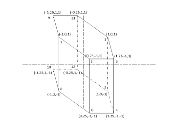
Figure 1: Polytope of problem 4.5.

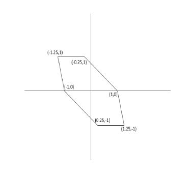
Figure 2: The projected figure of the polytope of Problem 4.5 in two dimensional space.

The projected figure of the polytope in x-y plane is depicted in Figure 2 which may help us to verify the result to be presented. First, let’s consider the $\{1,2\}$ edge. Given $i=1$ and $j=2$, i.e., ${\bf u}_{1}=[1,0,1]$ and ${\bf u}_{2}=[1,0,-1]$, it is not difficult (but tedious) to verify that the corresponding linear programming problem (16) can be written as

$$\begin{array}[]{cl}\min_{{\bf y},f}&f\\ s.t.&\left[\begin{array}[]{rrr}0.25&-1&1\\ 0.25&-1&-1\\ -0.75&-1&1\\ -0.75&-1&-1\\ -2&0&1\\ -2&0&-1\\ -2.25&1&1\\ -2.25&1&-1\\ -1.25&1&1\\ -1.25&1&-1\end{array}\right]\left[\begin{array}[]{c}y_{1}-1\\ y_{2}\\ y_{3}\end{array}\right]\leq\left[\begin{array}[]{c}f\\ f\\ f\\ f\\ f\\ f\\ f\\ f\end{array}\right],\\ &[0,~{}0,~{}-2][y_{1},~{}y_{2},~{}y_{3}]^{{\rm T}}=0,\\ &\left[\begin{array}[]{c}0\\ -1\\ -1\end{array}\right]\leq\left[\begin{array}[]{c}y_{1}\\ y_{2}\\ y_{3}\end{array}\right]\leq\left[\begin{array}[]{c}2\\ 1\\ 1\end{array}\right]\end{array}$$ (24)

which has the optimal solution ${\bf y}^{*}=[2,~{}0.75,~{}0]$ and $f^{*}=-0.5$. In addition, $c={\bf h}^{{\rm T}}[1,~{}0,~{}0]^{{\rm T}}=[1,~{}0.75,~{}0][1,~{}0,~{}0]^{{\rm T}}=1$. According to Theorem 2.2.(a), the line segment $\{1,2\}$ is an edge. Using the same strategy, we can determine that $\{5,6\}$, $\{7,8\}$, and $\{11,12\}$ are also edges. Algorithm 2.1 finds the H-representation as

$${\bf H}=\left[\begin{array}[]{rrrr}0&0&1\\ 1&0.25&0\\ 0&-1&0\\ -1&-1.25&0\\ -1&-0.25&0\\ 0&1&0\\ 1&1.25&0\\ 0&0&-1\end{array}\right]\hskip 7.22743pt{\bf b}=\left[\begin{array}[]{c}1\\ 1\\ 1\\ 1\\ 1\\ 1\\ 1\\ 1\end{array}\right]\hskip 7.22743pt$$

In summary, for all tested convex polytopes with known H-representations and V-representation, the algorithm is verified to be successful.

5 Conclusion

In this paper, an intuitive and novel facet enumeration algorithm is proposed. The idea is purely based on geometric observation, therefore, it is easy to understand. The out loop of algorithm is based on breadth-first search which eventually covers all the vertices of the polytope. The inner loop of the algorithm is based on depth-first search which will find the facets associated with the vertex under the consideration. The algorithm is implemented in Matlab and numerical test shows the efficiency and effectiveness of the algorithm. Due to the duality between the vertex enumeration problem and facet enumeration problem, we expect that this method can also be used to solve the vertex enumeration problem with some minor tweaks.

6 Acknowledgment

The author thanks an anonymous reviewer for pointing out a critical error in the previous version of this paper and for many of his comments, that are very helpful for the revision of this paper.

References

- [1] D. Avis, http://cgm.cs.mcgill.ca/ avis/C/lrs.html
- [2] D. Avis and K. Fukuda, (1992), A pivoting algorithm for convex hull and vertex enumeration of arrangements and polyhedra, Discrete Comput. Geom, 8(3):295 – 313.
- [3] D. Avis and C. Jordan, (2018), mplrs: A scalable parallel vertex/facet enumeration code, Mathematical Programming Computation, 10(2): 267–302.
- [4] R. G. Bland, (1977) New Finite Pivoting Rules for the Simplex Method, Mathematics Operations Research, 2: 103-107.
- [5] D. Bremner, K. Fukuda,and A. Marzetta, (1998), Primal-dual methods for vertex and facet enumeration. Discrete Comput. Geom., 20(3):333 – 357.
- [6] D. R. Chand and S. S. Kapur, (1970), An algorithm for convex polytopes, J. Assoc. Comput. Mach., 17(78):78 – 86.
- [7] G. Ceder, G. Garbulsky, D. Avis, K. Fukuda, (1994) Ground states of a ternary fcc lattice model with nearest- and next-nearest-neighbor interactions. Phys Rev B Condens Matter 49(1), 1–7.
- [8] G.B. Dantzig, Linear programming and extension, Princeton University Press, New Jersey, 1963.
- [9] M.M. Deza, M. Laurent, Geometry of cuts and metrics, Springer, New York, 1997.
- [10] M.E. Dyer, The complexity of vertex enumeration methods, Mathematics of Operations Research, 8: 381-402, 1983.
- [11] K. Fukuda and V. Rosta, (1994), Combinatorial face enumeration in convex polytopes, Computational Geometry: Theory and Applications, 4: 191-198.
- [12] T.S. Motzkin, H. Raiffa, G.L. Thompson, and R. M. Thrall, The Double Description Method, Annals of Math. Studies 8, pp. 51-73, Princeton University Press, 1953.
- [13] G. F. Swart, (1985), Finding the convex hull facet by facet, J. Algorithms, 6:17 – 48.
- [14] S. Wright, Primal-dual interior-point methods, SIAM, Philadelphia, 1997.
- [15] Y. Yang, Arc-search techniques for interior-point method, CRC Press, Florida, 2020.
- [16] G.M. Ziegler, Lectures on polytopes, Springer, New York, 1995.