Efficient Large-Scale Multi-Drone Delivery Using Transit Networks
Abstract
We consider the problem of controlling a large fleet of drones to deliver packages simultaneously across broad urban areas. To conserve energy, drones hop between public transit vehicles (e.g., buses and trams). We design a comprehensive algorithmic framework that strives to minimize the maximum time to complete any delivery. We address the multifaceted complexity of the problem through a two-layer approach. First, the upper layer assigns drones to package delivery sequences with a near-optimal polynomial-time task allocation algorithm. Then, the lower layer executes the allocation by periodically routing the fleet over the transit network while employing efficient bounded-suboptimal multi-agent pathfinding techniques tailored to our setting. Experiments demonstrate the efficiency of our approach on settings with up to drones, packages, and transit networks with up to stops in San Francisco and Washington DC. Our results show that the framework computes solutions typically within a few seconds on commodity hardware, and that drones travel up to of their flight range with public transit.
I Introduction
Rapidly growing e-commerce demands have greatly strained dense urban communities by increasing delivery truck traffic and slowing operations and impacting travel times for public and private vehicles [26, 24]. Further congestion is being induced by newer services relying on ride-sharing vehicles. There is a clear need to redesign the current method of package distribution in cities [29]. The agility and aerial reach of drones, the flexibility and ease of establishing drone networks, and recent advances in drone capabilities make them highly promising for logistics networks [28]. However, drones have limited travel range and carrying capacity [45, 14]. On the other hand, ground-based transit networks have less flexibility but greater coverage and throughput. By combining the strengths of both, we can achieve significant commercial benefits and social impact (e.g., reducing ground congestion and delivering essentials).

We address the problem of operating a large number of drones to deliver multiple packages simultaneously in an area. The drones can use one or more vehicles in a public-transit network as modes of transportation, thereby saving their limited battery energy stored onboard and increasing their effective travel range. We are required to decide which deliveries each drone should make and in what order, which modes of transit to use, and for what duration (Figure 1).
Our approach must contend with the multiple significant challenges of our problem. It must plan over large time-dependent transit networks, while accounting for energy constraints that limit the drones’ flight ranges. It must avoid inter-drone conflicts, such as where more than one drone attempts to board the same vehicle at the same time, or when the maximum carrying capacity of a vehicle is exceeded. We seek not just feasible multi-agent plans but high-quality solutions in terms of a cumulative objective over all drones, the makespan, i.e., the maximum individual delivery time for any drone. Additionally, our approach must also solve the task allocation problem of determining which drones deliver which packages, and from which distribution centers.
I-A Related work
Some individual aspects of our problem have already been studied. Choudhury et al. [10] investigated the single-agent setting of controlling a drone to use multiple modes of transit en route to its destination. Recent work has considered pairing a drone with a delivery truck, which does not exploit public transit [36, 2, 18]. The multi-agent issues of task allocation and inter-agent conflicts were not addressed either. Our problem is closely related to routing a fleet of autonomous vehicles providing mobility-on-demand services [44, 27, 47]. Specifically, the task is to compute routes for the vehicles (both customer-carrying and empty) so that travel demand is fulfilled and operational cost is minimized. In particular, recent works study the combination of such service with public transit, where passengers can use several modes of transportation in the same trip [40, 50]. However, such works abstract away inter-agent constraints or dynamics and are not suited for autonomous pathfinding. The task-allocation setting we consider in our problem can be viewed as an instance of the vehicle routing problem [8, 37, 46], variants of which are typically solved by mixed integer linear programming (MILP) formulations that scale poorly, or by heuristics without optimality guarantees.
We must contend with the challenges of planning for multiple agents. Accordingly, the second layer of our approach is a multi-agent path finding (MAPF) problem [16, 48]. Since the drones are on the same team, we have a centralized or cooperative pathfinding setting [42]. The MAPF problem is NP-hard to solve optimally [49]. A number of efficient solvers have been developed that work well in practice [17]. The MAPF formulation and algorithms have been extended to several relevant scenarios such as lifelong pickup-and-delivery [33] and joint task assignment and pathfinding [25, 32], though for different task settings and constraints than ours. Also, a MAPF formulation was applied for UAV traffic management in cities [23]. However, none of the approaches considered pathfinding over large time-dependent transit networks. We use models, algorithms and techniques from transportation planning [39, 13, 6].
I-B Statement of contributions
We present a comprehensive algorithmic framework for large-scale multi-drone delivery in synergy with a ground transit network. Our approach strives to minimize the maximum time to complete any delivery. We decompose the highly challenging problem and solve it stage-wise with a two-layer approach. First, the upper layer assigns drones to package-delivery sequences with a task allocation algorithm. Then, the lower layer executes the allocation by periodically routing the fleet over the transit network.
Algorithmically, we develop a new delivery sequence allocation method for the upper layer that obtains a near-optimal solution in polynomial runtime. For the lower layer, we extend techniques for multi-agent path finding that account for time-dependent transit networks and agent energy constraints to perform multi-drone routing. Experimentally, we present results supporting the efficiency of our approach on settings with up to drones, packages, and transit networks of up to stops in San Francisco and the Washington DC area. Our framework can compute solutions within a few seconds (up to minutes for the largest settings) on commodity hardware, and in our problem scenarios, drones can travel up to of their flight range using transit.
The following is the paper structure. We present an overall description of the two-layer approach in Section II, and then elaborate on each layer in Sections III and IV. We present experimental results on simulations in Section V, and conclude the paper with Section VI.
II Methodology
We provide a high-level description of our formulation and approach to illustrate the various interacting components.
II-A Problem Formulation
We are operating a centralized homogeneous fleet of drones within a city-scale domain. There are product depots with known geographic locations, denoted by . The depots are both product dispatch centers and drone-charging stations. At the start of a large time interval (e.g., a day), a batch of delivery request locations for different packages, denoted , is received (we assume that ). We assume that any package can be dispatched from any depot; our framework exploits this property to optimize the solution quality in terms of makespan, i.e., the maximum execution time for any delivery. In Section III, we mention how our approach can accommodate dispatch constraints.
The drones carry packages from depots to delivery locations. They can extend their effective travel range by using public transit vehicles in the area, which remain unaffected by the drones’ actions. Our problem is to route drones to deliver all packages while minimizing makespan. A drone route consists of its current location and the sequence of depot and package locations to visit with a combination of flying and riding on transit. We characterize the drones’ limited energy as a maximum flight distance constraint. A feasible solution must satisfy inter-drone constraints such as collision avoidance and transit vehicle capacity limits.
Finally, we make some assumptions for our setting: a drone carries one package at a time, which is reasonable given state-of-the-art drone payloads [14]; drones are recharged upon visiting a depot in negligible time (e.g., a battery replacement); depots have unlimited drone capacity; the transit network is deterministic with respect to locations and vehicle travel times (we mention uncertainty in Section VI). We do account for the time-varying nature of the transit.
II-B Approach overview
In principle, we could frame the entire problem as a mixed integer linear program (MILP). However, for real-world problems (hundreds of drones; thousands of packages; large transit networks), even state-of-the-art MILP approaches are unlikely to scale. Moreover, even a simpler problem that ignores the interaction constraints is an instance of the notoriously challenging multi-depot vehicle routing problem [37]. Thus, we decouple the problem into two distinct subproblems that we solve stage-wise in layers.
The upper layer performs task allocation to determine which packages are delivered by which drone and in what order. It takes as input the known depot and package locations, and an estimate of the drone travel time between every pair of locations. It then solves a threefold allocation to minimize delivery makespan and assigns to each package (i) the dispatch depot and (ii) the delivery drone, and to each drone (iii) the order of package deliveries. To this end, we develop an efficient polynomial-time task-allocation algorithm that achieves a near-optimal makespan.
The lower layer performs route planning for the drone fleet to execute the allocated delivery tasks. It generates detailed routes of drone locations in time and space and the transit vehicles used, while accounting for the time-varying transit network. It also ensures that (i) simultaneous transit boarding by multiple drones is avoided, (ii) no transit vehicle exceeds its drone-carrying capacity, and (iii) drone (battery) energy constraints are respected. We efficiently handle individual and inter-drone constraints by framing the routing problem as an extension of multi-agent path finding (MAPF) to transit networks. We adapt a scalable, bounded sub-optimal variant of a highly effective MAPF solver called Conflict-Based Search (CBS) [41] to solve the one-delivery-per-drone problem. Finally, we obtain routes for the sequence of deliveries in a receding-horizon fashion by replanning for the next task once a drone completes its current one.
Decomposition-based stage-wise optimization approaches typically have an approximation gap compared to the optimal solution of the full problem. For us, this gap manifests in the surrogate cost estimate we use for the drone’s travel time in the task-allocation layer (instead of jointly solving for allocation and multi-agent routing over transit networks, which is not feasible at scale). The better the surrogate, the more coupled the layers are, i.e., the better is the solution of the first stage for the second one. Such surrogates have a tradeoff between efficiency and approximation quality. An easy-to-compute travel time surrogate, for instance, is the drone’s direct flight time between two locations (ignoring transit). However, that can be poor-quality when the drone requires transit for an out-of-range target. We use a surrogate that actually accounts for the transit network, at the expense of some modest preprocessing. We defer details to Appendix C, but the idea is to precompute the pairwise shortest travel times between locations spread around the city, over a representative snapshot of the transit network.
III Task Assignment and Package Allocation
We leverage our problem’s structure to design a new algorithm called MergeSplitTours for the task-allocation layer, which guarantees a near-optimal solution in polynomial time. The goal of this layer is to (i) distribute the set of packages among agents, (ii) assign each package destination to a depot , and (iii) assign drones to a sequence of depot pickups and package deliveries. The objective is to minimize the maximum travel time among all agents over all three of the above components.
Our problem can be cast as a special version of the traveling salesman problem [7], which we call the minimal visiting paths problem (-MVP). We seek a set of paths such that the makespan, i.e., the maximum travel time for any path, is minimized. We only need paths that start and end at (the same or different) depots, not tours. Our formulation is a special case of the the asymmetric variant, for a directed underlying graph, which is NP-hard even for on general graphs [4] (although it is not known whether the specific instance of our problem is NP-hard as well). Moreover, the current best polynomial-time approximation [4] yields the fairly large approximation factor , for a graph with vertices. An additional challenge is the inability to assume the triangle inequality on our objective of travel times.
A key element of -MVP is the allocation graph , with vertex set . Each directed edge is weighted according to an estimated travel time from the location of to that of in the city. For every we exclude the edge from if it is impossible to reach from while using at most of the flight range allowed (similarly for edges). As we flagged in Section II-B, any dispatch constraints are modeled by excluding edges from the corresponding depot. We are now ready for the full definition of -MVP:
Given allocation graph , with , (1) subject to (2) (3) (4) (5) where denote the in and out going neighbors of .
Definition 1.
Given allocation graph , the minimal visiting paths problem (-MVP) consists of finding paths on , such that (1) each path starts at some depot and terminates at the same or different , (2) exactly one path visits each package , and (3) the maximum travel time of any of the paths is minimized.
Let opt be the optimal makespan, i.e., , where denotes the total travel time along a given path or tour. We make three observations. First, if a path contains the sub-path , for some , then should be dispatched from depot and the drone delivering will return to after delivery. Second, a package being found in indicates that drone should deliver it. Third, fully characterizes the order of packages delivered by drone .

III-A Algorithm Overview
We present our MergeSplitTours algorithm for solving -MVP (Algorithm 1); see a detailed description in Appendix A. A key step is generating an initial set of tours by solving the minimal-connecting tours (MCT) problem (see Table I), which attempts to connect packages to depots within tours to minimize the total edge weight in eq. 1. The constraint in eq. 4 is that each package is connected to precisely one incoming and one outgoing edge from and to depots respectively. The final constraint in eq. 5 enforces inflow and outflow equality for every depot. Edges connecting packages can be used at most once, whereas edges connecting depots can be used multiple times. The solution to MCT is the assignment , i.e., which edges of are used and how many times. This assignment implicitly represents the desired collection of the tours ; see Appendix A.
III-B Theoretical Guarantees
All proofs from this secion are in Appendix A. The following theorem states that MergeSplitTours is correct and that its makespan is close to optimal.
Theorem 1.
Suppose is strongly connected and the subgraph induced by the vertices is a directed clique. Let be the output of MergeSplitTours. Then, every package is contained in exactly one path , and every starts and ends at a depot. Moreover, holds,
The key idea is that the total cost of the tours induced by the solution to MCT cannot exceed the total length of . The MCT solution is then adapted to paths with an additional overhead of per path. When (typically the case), are small compared to opt, making the bound tight. For instance, in our randomly-generated scenarios in Section V-A, for , the approximation ratio , and for , the factor is .
The computational bottleneck of the algorithm is MCT, while the other components can clearly be implemented polynomially in the input size. However, it suffices to solve a relaxed version of MCT to obtain the same integral solution.
Lemma 1.
The optimal solution to the fractional relaxation of MCT, in which for all , and otherwise, yields the integer optimal solution.
The lemma follows from casting MCT as the minimum-cost circulation problem, for which the constraint matrix is totally unimodular [3]. Therefore, MergeSplitTours can be implemented in polynomial time.
IV Multi-Agent Path Finding
For each drone , the allocation layer yields a sequence of delivery tasks . Each delivery sequence has one or more subsequences of . The route-planning layer treats each subsequence as an individual drone task, i.e., leaving with the package from depot , carrying it to package location and returning to the (same or different) depot , without exceeding the energy capacity. We seek an efficient and scalable method to obtain high-quality (with respect to travel time) feasible paths, while using transit options to extend range, for different drone tasks simultaneously. The full set of delivery sequences can be satisfied by replanning when a drone finishes its current task and begins a new one; we discuss and compare two replanning strategies in Appendix D. Thus, we formulate the problem of multi-drone routing to satisfy a set of delivery sequences as receding-horizon multi-agent path finding (MAPF) over transit networks. In this section, we describe the graph representation of our problem and present an efficient bounded sub-optimal algorithm.
IV-A MAPF with Transit Networks (MAPF-TN)
The problem of Multi-Agent Path Finding with Transit Networks (MAPF-TN) is the extension of standard MAPF to where agents can use one or more modes of transit in addition to moving. The incorporation of transit networks introduces additional challenges and underlying structure. The input to MAPF-TN is the set of tasks and the directed operation graph . In Section III, the allocation graph only considered depots and packages, and edges between them. Here, also includes transit vertices, , where is the set of trips, and each trip is a sequence of time-stamped stop locations (a given stop location may appear as several different nodes with distinct time-stamps). Similarly, we also use time-expanded versions of and [39].
The edges are defined as follows: An edge is a transit edge if and are consecutive stops on the same trip . Any other edge is a flight edge. An edge is time-constrained if and time-unconstrained otherwise. Every edge has three attributes: traversal time , energy expended , and capacity . Since each vertex is associated with a location, denotes the distance between them for a suitable metric. MAPF typically abstracts away agent dynamics; we have a simple model where drones move at constant speed , and distance flown represents energy expended. Due to high graph density (drones can fly point-to-point between many stops), we do not explicitly enumerate edges but generate them on-the-fly during search.
We now define the three attributes for . For time-constrained edges, is the difference between corresponding time-stamps (if , is the chosen departure time), and for time-unconstrained edges, is the time of direct flight. For flight edges, (flight distance), and for transit edges, . For transit edges, is bounded by the capacity of the vehicle, while for flight edges, . Here, we assume that time-unconstrained flight in open space can be accommodated (thorougly examined in [23]).
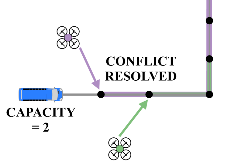
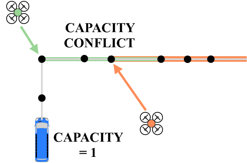
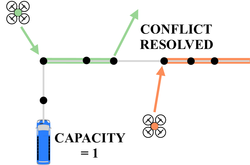
We now describe the remaining relevant MAPF-TN details. An individual path for drone from through to is feasible if the energy constraint is satisfied, where is the drone’s maximum flight distance. In addition, the drone should be able to traverse the distance of a time-constrained flight edge in time, i.e., . For simplicity, we abstract away energy expenditure due to hovering in place by flying the drone at reduced speed to reach the transit just in time. Thus, the constraint is only on the traversed distance. The cost of an individual path is the total traversal time, . A feasible solution is a set of individually feasible paths that does not violate any of the following two shared constraints (see Figure 2): (i) Boarding constraint, i.e., no two drones may board the same vehicle at the same stop; (ii) Capacity constraint, i.e., a transit edge may not be used by more than drones. As with the allocation layer, the global objective for MAPF-TN is to minimize the solution makespan, , i.e., minimize the worst individual completion time.
IV-B Conflict-Based Search for MAPF-TN
To tackle MAPF-TN, we modify the Conflict-Based Search (CBS) algorithm [41]. The multi-agent level of CBS identifies shared constraints and imposes corresponding path constraints on the single-agent level. The single-agent level computes optimal individual paths that respect all constraints. If individual paths conflict (i.e., violate a shared constraint), the multi-agent level adds further constraints to resolve the conflict, and invokes the single-agent level again, for the conflicting agents. In MAPF-TN, conflicts arise from boarding and capacity constraints. CBS obtains optimal multi-agent solutions without having to run (potentially significantly expensive) multi-agent searches. However, its performance can degrade heavily with many conflicts in which constraints are violated. Figure 2 illustrates the generation and resolution of conflicts in our MAPF-TN problem.
For scalability, we use a bounded sub-optimal variant of CBS called Enhanced CBS (ECBS), which achieves orders of magnitude speedups over CBS [5]. ECBS uses bounded sub-optimal Focal Search [38] at both levels, instead of best-first A* [22]. Focal search allows using an inadmissible heuristic that prioritizes efficiency. We now describe a crucial modification to ECBS required for MAPF-TN.
Focal Weight-constrained Search: Unlike typical MAPF, the low-level graph search in MAPF-TN has a path-wide constraint (traversal distance) in addition to the objective function of traversal time. For the shortest path problems on graphs, adding a path-wide constraint makes it NP-hard [20]. Several algorithms for constrained search require an explicit enumeration of the edges [15, 9]. We extend the A* for MultiConstraint Shortest Path (A*-MCSP) algorithm [31] (suitable for our implicit graph) to focal search (called Focal-MCSP). Focal-MCSP uses admissible heuristics on both objective and constraint and maintains only non-dominated paths to intermediate nodes. This extensive book-keeping requires a careful implementation for efficiency.
Focal-MCSP inherits the properties of A*-MCSP and Focal Search; therefore, it yields a bounded-suboptimal feasible path to the target. Accordingly, ECBS with Focal-MCSP yields a bounded sub-optimal solution to MAPF-TN. The result follows from the analysis of ECBS [5]. Also, note that a path requires a bounded sub-optimal path from to and another from to , such that their concatenation is feasible. Since this is even more complicated, in practice, we run Focal-MCSP twice (from to and to ) with half the energy constraint each time and concatenate the paths, guaranteeing feasibility. In Appendix B-B we discuss other required modifications to standard MAPF and important speedup techniques that nonetheless retain the bounded sub-optimality of Enhanced CBS for our MAPF-TN formulation.
| San Francisco | Washington DC | ||||||||
| Depots, Agents | Median, Avg | Avg Soln. | Median, Avg | Avg Soln. | |||||
| Plan Time | Range Ext. | Transit Used | Makespan | Plan Time | Range Ext. | Transit Used | Makespan | ||
V Experiments and Results
We implemented our approach using the Julia language and tested it on a machine with a -core RAM CPU.111The code for our work is available at https://github.com/sisl/MultiAgentAllocationTransit.jl. For very large combinatorial optimization problems, solution quality and algorithm efficiency are of interest. We have already shown that the upper and lower layers are near-optimal and bounded-suboptimal respectively in terms of solution quality, i.e., makespan. Therefore, for evaluation we focus on their efficiency and scalability to large real-world settings. We do not attempt to baseline against a MILP approach for the full problem; we estimate that a typical setting of interest will have on the order of variables in a MILP formulation, besides exponential constraints.
We ran simulations with two large-scale public transit networks in San Francisco (SFMTA) and the Washington Metropolitan Area (WMATA). We used the open-source General Transit Feed Specification data [1] for each network. We considered only the bus network (by far the most extensive), but our formulation can accommodate multiple modes. We defined a geographical bounding box in each case, of area for SFMTA and for WMATA (illustrated in Appendix D), within which depots and package locations were randomly generated. For the transit network, we considered all bus trips that operate within the bounding box. The size of the time-expanded network, , is the total number of stops made by all trips; for SFMTA and for WMATA (recall that edges are implicit, so varies between queries, but the full graph can be dense). The drone’s flight range constraint is set (conservatively) to and average speed to , based on the DJI Mavic 2 specifications [14]. In this section, we evaluate the two main components — the task allocation and multi-agent path finding layers. In Appendix D we compare the performance of two replanning strategies for when a drone finishes its current delivery, and two surrogate travel time estimates for coupling the layers.
V-A Task Allocation
The scale of the allocation problem is determined by the number of depots and packages, i.e., . The runtimes for MergeSplitTours with varying over SFMTA are displayed in Table II. The roughly quadratic increase in runtimes along a specific row or column demonstrate that our provably near-optimal MergeSplitTours algorithm is indeed polynomial in the size of the input. Even for up to deliveries, the absolute runtimes are quite reasonable. We do not compare with naive MILP even for allocation, as the number of variables would exceed , in addition to the expensive subtour elimination constraints [34].
V-B MAPF with Transit Networks (MAPF-TN)
Solving multi-agent path finding optimally is NP-hard [49]. Previous research has benchmarked CBS variants and shown that Enhanced CBS is most effective [5, 11]. Therefore, we focus on extensively evaluating our own approach rather than redundant baselining. Table III quantifies several aspects of the MAPF-TN layer with varying numbers of depots and agents , the two most tunable parameters. Before each trial, we run the allocation layer and collect tasks, one for each agent. We then run the MAPF-TN solver on this set of tasks to compute a solution.
We discuss broad observations here and provide a detailed analysis in Appendix D. The results are very promising; our approach scales to large numbers of agents () and large transit networks (nearly vertices); the highest average makespan for the true delivery time is less than an hour () for SFMTA and 2 hours () for WMATA; drones are using up to transit options per route to extend their range by up to x. As we anticipated, conflict resolution is a major bottleneck of MAPF-TN. A higher ratio of agents to depots increases conflicts due to shared transit, thereby increasing plan time (compare to ). A higher number of depots puts more deliveries within flight range of a depot, reducing conflicts, makespan, and the need for transit usage and range extension (compare to ). Plan times are much higher for WMATA due to a larger area and a larger and less uniformly distributed bus network, leading to higher single-agent search times and more multi-agent conflicts. Trials taking more than minutes were discarded; two pathological cases with SFMATA and WMATA (each with ) took nearly and minutes, due to and conflicts respectively. In any case, a deployed system would have better compute and parallelized implementations. Finally, note that the running times reported here are actually pessimistic, because we consider cases where drones are released simultaneously from the depots, which increases conflicts. However, a gradual release by executing the MAPF solver over a longer horizon (as we discuss in Appendix D-B) results in fewer conflicts, allowing us to cope with an even larger drone fleet.
VI Conclusion and Future Work
We designed a comprehensive algorithmic framework for solving the highly challenging problem of multi-drone package delivery with routing over transit networks. Our two-layer approach is efficient and highly scalable to large problem settings and obtains high-quality solutions that satisfy the many system constraints. We ran extensive simulations with two real-world transit networks that demonstrated the widespread applicability of our framework and how using ground transit judiciously allows drones to significantly extend their effective range.
A key future direction is to perform case studies that estimate the operational cost of our framework, evaluate its impact on road congestion, and consider potential externalities like noise pollution and disparate impact on urban communities. Another direction is to extend our model to overcome its limitations: delays and uncertainty in the travel pattern of transit vehicles [35] and delivery time windows [43]; jointly routing ground vehicles and drones; optimizing for the placements of depots, whose locations are currently randomly generated and given as input.
Acknowledgments
This work was supported in part by NSF, Award Number: 1830554, the Toyota Research Institute (TRI), and the Ford Motor Company. The authors thank Sarah Laaminach, Nicolas Lanzetti, Mauro Salazar, and Gioele Zardini for fruitful discussions on transit networks.
References
- [1] General Transit Feed Specification. URL https://developers.google.com/transit/gtfs/. Accessed: August 30, 2019.
- Agatz et al. [2018] Niels Agatz, Paul Bouman, and Marie Schmidt. Optimization Approaches for the Traveling Salesman Problem with Drone. Transportation Science, 52(4):965–981, 2018.
- Ahuja et al. [1993] Ravindra K. Ahuja, Thomas L. Magnanti, and James B. Orlin. Network Flows: Theory, Algorithms, and Applications. Pearson, 1993.
- Asadpour et al. [2017] Arash Asadpour, Michel X. Goemans, Aleksander Madry, Shayan Oveis Gharan, and Amin Saberi. An -Approximation Algorithm for the Asymmetric Traveling Salesman Problem. Operations Research, 65(4):1043–1061, 2017.
- Barer et al. [2014] Max Barer, Guni Sharon, Roni Stern, and Ariel Felner. Suboptimal Variants of the Conflict-based Search Algorithm for the Multi-agent Pathfinding Problem. In Symposium on Combinatorial Search, 2014.
- Bast et al. [2016] Hannah Bast, Daniel Delling, Andrew Goldberg, Matthias Müller-Hannemann, Thomas Pajor, Peter Sanders, Dorothea Wagner, and Renato F Werneck. Route Planning in Transportation Networks. In Algorithm Engineering, pages 19–80. Springer, 2016.
- Bektas [2006] Tolga Bektas. The Multiple Traveling Salesman Problem: an Overview of Formulations and Solution Procedures. Omega, 34(3):209–219, 2006.
- Caceres-Cruz et al. [2014] Jose Caceres-Cruz, Pol Arias, Daniel Guimarans, Daniel Riera, and Angel A. Juan. Rich Vehicle Routing Problem: Survey. ACM Comput. Surv., 47(2):32:1–32:28, 2014.
- Carlyle et al. [2008] W Matthew Carlyle, Johannes O Royset, and R Kevin Wood. Lagrangian Relaxation and Enumeration for Solving Constrained Shortest-Path Problems. Networks, 52(4):256–270, 2008.
- Choudhury et al. [2019] Shushman Choudhury, Jacob P. Knickerbocker, and Mykel J. Kochenderfer. Dynamic Real-time Multimodal Routing with Hierarchical Hybrid Planning. In IEEE Intelligent Vehicles Symposium (IV), pages 2397–2404, 2019.
- Cohen et al. [2016] Liron Cohen, Tansel Uras, TK Satish Kumar, Hong Xu, Nora Ayanian, and Sven Koenig. Improved Solvers for Bounded-Suboptimal Multi-Agent Path Finding. In International Joint Conference on Artificial Intelligence (IJCAI), pages 3067–3074, 2016.
- Cormen et al. [2009] Thomas H. Cormen, Charles E. Leiserson, Ronald L. Rivest, and Clifford Stein. Introduction to Algorithms. MIT Press, 2009.
- Delling et al. [2009] Daniel Delling, Peter Sanders, Dominik Schultes, and Dorothea Wagner. Engineering Route Planning Algorithms. In Algorithmics of Large and Complex Networks, pages 117–139. Springer-Verlag, 2009.
- [14] DJI. DJI Mavic 2 Specifications Sheet. URL http://bit.ly/2mfCAvz.
- Dumitrescu and Boland [2003] Irina Dumitrescu and Natashia Boland. Improved Preprocessing, Labeling and Scaling Algorithms for the Weight-Constrained Shortest Path Problem. Networks: An International Journal, 42(3):135–153, 2003.
- Erdmann and Lozano-Perez [1987] Michael Erdmann and Tomas Lozano-Perez. On Multiple Moving Objects. Algorithmica, 2(1-4):477, 1987.
- Felner et al. [2017] Ariel Felner, Roni Stern, Solomon Eyal Shimony, Eli Boyarski, Meir Goldenberg, Guni Sharon, Nathan Sturtevant, Glenn Wagner, and Pavel Surynek. Search-based Optimal Solvers for the Multi-Agent Pathfinding Problem: Summary and Challenges. In Symposium on Combinatorial Search, 2017.
- Ferrandez et al. [2016] Sergio Mourelo Ferrandez, Timothy Harbison, Troy Weber, Robert Sturges, and Robert Rich. Optimization of a Truck-Drone in Tandem Delivery Network using k-means and Genetic Algorithm. Journal of Industrial Engineering and Management, 9(2):374–388, 2016.
- Frederickson et al. [1976] Greg N. Frederickson, Matthew S. Hecht, and Chul E. Kim. Approximation Algorithms for some Routing Problems. In 17th Annual Symposium on Foundations of Computer Science, Houston, Texas, USA, 25-27 October 1976, pages 216–227, 1976.
- Garey and Johnson [1990] Michael R Garey and David S Johnson. Computers and Intractability; A Guide to the Theory of NP-Completeness. WH Freeman & Co., 1990.
- Halton [1960] John H Halton. On the Efficiency of certain Quasi-Random Sequences of Points in Evaluating Multi-Dimensional Integrals. Numerische Mathematik, 2(1):84–90, 1960.
- Hart et al. [1968] Peter Hart, Nils Nilsson, and Bertram Raphael. A Formal Basis for the Heuristic Determination of Minimum Cost Paths. IEEE Transactions on Systems Science and Cybernetics, 2(4):100–107, 1968.
- Ho et al. [2019] Florence Ho, Ana Salta, Ruben Geraldes, Artur Goncalves, Marc Cavazza, and Helmut Prendinger. Multi-agent Path Finding for UAV Traffic Management. In International Conference on Autonomous Agents and Multiagent Systems (AAMAS), pages 131–139, 2019.
- Holguin-Veras et al. [2018] Jose Holguin-Veras, Johanna Amaya Leal, Ivan Sanchez-Diaz, Michael Browne, and Jeffrey Wojtowicz. State of the art and Practice of Urban Freight Management: Part I: Infrastructure, Vehicle-Related, and Traffic Operations. Transportation Research Part A: Policy and Practice, 2018.
- Hönig et al. [2018] Wolfgang Hönig, Scott Kiesel, Andrew Tinka, Joseph W Durham, and Nora Ayanian. Conflict-based Search with Optimal Task Assignment. In International Conference on Autonomous Agents and Multiagent Systems (AAMAS), pages 757–765, 2018.
- Humes [2018] Edward Humes. Online Shopping Was Supposed to Keep People Out of Traffic. It Only Made Things Worse, 2018. URL http://bit.ly/2HCkAmQ. Accessed: August 30, 2019.
- Iglesias et al. [2019] Ramón Iglesias, Federico Rossi, Rick Zhang, and Marco Pavone. A BCMP network approach to modeling and controlling autonomous mobility-on-demand systems. I. J. Robotics Res., 38(2-3), 2019.
- Joerss et al. [2016] Martin Joerss, Florian Neuhaus, and Jurgen Schroder. How Customer Demands are Reshaping Last-Mile Delivery, 2016. URL https://mck.co/2NIRdmE. Accessed: August 30, 2019.
- Kafle et al. [2017] Nabin Kafle, Bo Zou, and Jane Lin. Design and Modeling of a Crowdsource-Enabled System for Urban Parcel Relay and Delivery. Transportation Research Part B: Methodological, 99:62 – 82, 2017. ISSN 0191-2615.
- Kung et al. [1975] Hsiang-Tsung Kung, Fabrizio Luccio, and Franco P Preparata. On Finding the Maxima of a Set of Vectors. Journal of the ACM (JACM), 22(4):469–476, 1975.
- Li et al. [2007] Yuxi Li, Janelee Harms, and Robert Holte. Fast Exact Multiconstraint Shortest Path Algorithms. In IEEE International Conference on Communications, pages 123–130, 2007.
- Liu et al. [2019] Minghua Liu, Hang Ma, Jiaoyang Li, and Sven Koenig. Task and Path Planning for Multi-Agent Pickup and Delivery. In International Conference on Autonomous Agents and Multiagent Systems (AAMAS), pages 1152–1160, 2019.
- Ma et al. [2017] Hang Ma, Jiaoyang Li, TK Kumar, and Sven Koenig. Lifelong Multi-agent Path Finding for Online Pickup and Delivery Tasks. In International Conference on Autonomous Agents and Multiagent Systems (AAMAS), pages 837–845, 2017.
- Miller et al. [1960] Clair E Miller, Albert W Tucker, and Richard A Zemlin. Integer Programming Formulation of Traveling Salesman Problems. Journal of the ACM (JACM), 7(4):326–329, 1960.
- Müller-Hannemann et al. [2007] Matthias Müller-Hannemann, Frank Schulz, Dorothea Wagner, and Christos Zaroliagis. Timetable Information: Models and Algorithms. In Algorithmic Methods for Railway Optimization, pages 67–90. Springer, 2007.
- Murray and Chu [2015] Chase C. Murray and Amanda G. Chu. The Flying Sidekick Traveling Salesman Problem: Optimization of Drone-Assisted Parcel Delivery. Transportation Research Part C: Emerging Technologies, 54:86 – 109, 2015.
- Otto et al. [2018] Alena Otto, Niels Agatz, James Campbell, Bruce Golden, and Erwin Pesch. Optimization Approaches for Civil Applications of Unmanned Aerial Vehicles (uavs) or Aerial Drones: A Survey. Networks, 72(4):411–458, 2018.
- Pearl and Kim [1982] Judea Pearl and Jin H Kim. Studies in Semi-Admissible Heuristics. IEEE Transactions on Pattern Analysis and Machine Intelligence, (4):392–399, 1982.
- Pyrga et al. [2008] Evangelia Pyrga, Frank Schulz, Dorothea Wagner, and Christos Zaroliagis. Efficient Models for Timetable Information in Public Transportation Systems. Journal of Experimental Algorithmics (JEA), 12:2–4, 2008.
- Salazar et al. [2018] Mauro Salazar, Federico Rossi, Maximilian Schiffer, Christopher H. Onder, and Marco Pavone. On the interaction between autonomous mobility-on-demand and public transportation systems. In International Conference on Intelligent Transportation Systems, pages 2262–2269, 2018.
- Sharon et al. [2012] Guni Sharon, Roni Stern, Ariel Felner, and Nathan Sturtevant. Conflict-based Search for Optimal Multi-Agent Path Finding. In AAAI Conference on Artificial Intelligence (AAAI), 2012.
- Silver [2005] David Silver. Cooperative Pathfinding. In AAAI Conference on Artificial Intelligence (AAAI), pages 117–122, 2005.
- Solomon [1987] Marius M Solomon. Algorithms for the Vehicle Routing and Scheduling Problems with Time Window Constraints. Operations Research, 35(2):254–265, 1987.
- Solovey et al. [2019] Kiril Solovey, Mauro Salazar, and Marco Pavone. Scalable and Congestion-Aware Routing for Autonomous Mobility-On-Demand via Frank-Wolfe Optimization. In Proceedings of Robotics: Science and Systems, 2019.
- Sudbury and Hutchinson [2016] Adrienne Welch Sudbury and E Bruce Hutchinson. A Cost Analysis of Amazon Prime Air (Drone Delivery). Journal for Economic Educators, 16(1):1–12, 2016.
- Toth and Vigo [2014] P. Toth and D. Vigo. Vehicle Routing – Problems, Methods, and Applications. SIAM, 2 edition, 2014.
- Wallar et al. [2018] Alex Wallar, Menno Van Der Zee, Javier Alonso-Mora, and Daniela Rus. Vehicle rebalancing for mobility-on-demand systems with ride-sharing. In IEEE/RSJ International Conference on Intelligent Robots and Systems, pages 4539–4546, 2018.
- Yu and LaValle [2016] J. Yu and S. M. LaValle. Optimal Multirobot Path Planning on Graphs: Complete Algorithms and Effective Heuristics. IEEE Transactions on Robotics, 32(5):1163–1177, 2016.
- Yu and LaValle [2013] Jingjin Yu and Steven M LaValle. Structure and Intractability of Optimal Multi-robot Path Planning on Graphs. In AAAI Conference on Artificial Intelligence (AAAI), 2013.
- Zgraggen et al. [2019] J. Zgraggen, M. Tsao, M. Salazar, M. Schiffer, and M. Pavone. A Model Predictive Control Scheme for Intermodal Autonomous Mobility-on-Demand. In IEEE International Conference on Intelligent Transportation Systems, 2019.
Appendix A Task Allocation: Additional Details and Proofs
We present a full and extended version of the MergeSplitTours algorithm (Algorithm 2) for the task allocation layer. Figure 3 illustrates the behaviour of MCT, which provides an approximate solution for the -MVP problem (Definition 1). The algorithm consists of three main steps:

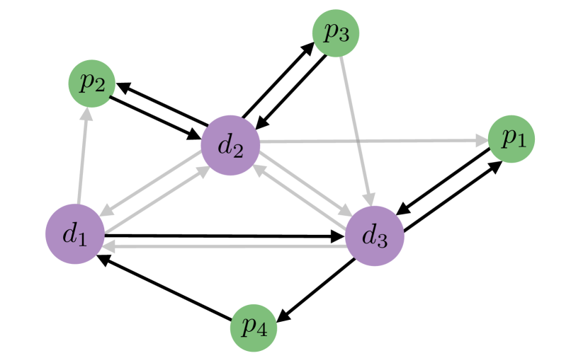

Step 1 (lines 1): Generate a collection of tours , for some , such that every package is covered by exactly one tour, and the total distance of the tours is minimized. This step is achieved by solving the minimal-connecting tours (MCT) problem (see Table I). The solution to MCT is given by an assignment , which indicates which edges of are used and for how many times. This assignment implicitly represents the desired collection of tours , as described above. The reason behind why such an assignment breaks into a collection of tours is discussed in Lemma 2 below.
Step 2 (lines 2-10): The tours are merged in an iterative fashion, until a single tour is generated. We first identify connected depot sets , which are induced by the MCT solution (line 2). That is, every consists of all the depots that belong to one specific tour encoded by . We then perform a merging routine which merges the tours and consequently merges the connected depot sets. This routing iterates over all combinations of (lines 5-8), and chooses , such that is minimized. Then and are updated accordingly (lines 9, 10). For a given and , the notation represents the depot component that belongs to.
Step 3 (lines 6-14): The tour is partitioned into paths such that the length of every path is proportional to the length of divided by . Additionally, every path starts and ends in a depot, but not necessarily the same one. This step is reminiscent to an algorithm presented in [19] for -TSP in undirected graphs.
A-A Completeness and optimality
In preparation to the proof Theorem 1, we have the following lemma, which states that MCT produces a collection of pairwise-disjoint tours. Henceforth we assume that that is strongly connected and that is a directed clique.
Lemma 2.
Let be the output of . Then there exists a collection of vertex-disjoint tours , such that for every such that , there exists in which appears exactly times.
Proof.
By definition of MCT, for every there exists precisely one incoming edge and one outgoing edge such that . Also, note that by Equation 5, the in-degree and out-degree of every are equal to each other. Thus, an Eulerian tour can be formed, which traverses every edge exactly times. ∎
We are ready for the main proof.
Proof of Theorem 1.
First, note that after every iteration of the “while” loop, the updated assignment still represents a collection of tours. Second, this loop is repeated at most times; , which represents the initial number of connected depots (line 2), is at most , since every tour induced by MCT must contain at least one depot.
Next, let opt be the optimal solution to -MVP. That is, there exists paths which represent the solution to -MVP, and for every , . Observe that
where is the result of MergeSplitTours. Next, by definition of , we have that . Lastly, by definition of we have that
A-B Computational complexity
We conclude this section with an analysis of the computational complexity of MergeSplitTours. Recall that we identified the main bottleneck of MergeSplitTours to be the solution computation for MCT. We proceed to prove Lemma 1, which states such a solution to MCT can be obtained via a linear relaxation.
Proof.
The main observation to make is that can be transformed into a minimum-cost circulation (MCC) problem. If all edge capacities are integral, the linear relaxation of MCC enjoys a totally unimodular constraint matrix form [3]. Hence, the linear relaxation will necessarily have an integer optimal solution, which will be a fortiori an optimal solution to the original MCF problem.
In the current representation of MCT, eq. 4 does not correspond to a circulation problem. However, we can introduce a small modification to which would allow us to recast it as circulation. Consider the graph such that
and we require that for every such , . ∎
Appendix B MAPF-TN: Additional Details
We now elaborate on two aspects of multi-agent pathfinding with transit networks (MAPF-TN) that we alluded to in Section IV. First, we discuss how we extend the notion of conflict handling in Conflict-Based Search to the capacity conflicts of MAPF-TN, where more than one agent can use a transit edge. Second, we discuss two important speedup techniques that improve the empirical performance of our MAPF-TN solver, without sacrificing bounded suboptimality.
B-A Capacity Conflicts in (E)CBS
In the classical MAPF formulation, at most one agent can occupy a particular vertex or traverse a particular edge at a given time. Therefore, conflicts between agents yield new nodes in the multi-agent level search tree of Conflict-Based Search (CBS) and any of its modified variants. In MAPF-TN, however, transit edges in general have capacity . Consider a solution generated during a run of Enhanced CBS that has assigned to some transit edge drones. In order to guarantee bounded sub-optimality of the solution, we must generate all sets of constraints, where . Each such set of constraints represents one subset of agents being restricted from using the transit edge in question.
As we pointed out in Section V-B, conflict resolution is a significant bottleneck for solving large MAPF-TN instances. In our experiments, we generated all constraint subsets of a capacity conflict, however, pathological scenarios may arise where this significantly degrades performance in practice (our ultimate yardstick). Whether there exists a principled way to analyse constraint set enumeration and suboptimality and how this can be efficiently implemented in practice are both important questions for future research.
B-B Speedup Techniques
The NP-hardness of multi-agent path finding [49] and the additional computational challenges of MAPF-TN (path energy constraint; large and dense graphs) make empirical performance paramount, given our real-world scenarios and emphasis on scalability. We now discuss some speedup techniques that improve the efficiency of the low-level search while maintaining its bounded sub-optimality (which in turn ensures bounded sub-optimality of the overall solution, as per Enhanced CBS). Certainly, these techniques are not exhaustive; there is an entire body of work in transportation planning devoted to speeding up algorithm running times [13]. We devised and implemented two simple methods.
B-B1 Preprocessing Public Transit Networks
Focal-MCSP can become a bottleneck when it has to be run multiple times (at least twice for each agent’s current task and more in case of conflicts). Its performance depends significantly on the availability and quality of admissible heuristics, i.e., heuristics that underestimate the cost to the goal, for the objective (elapsed time) and constraint (distance traversed, a surrogate for the energy expended). The public-transit network for a given area is usually known in advance and follows a pre-determined timetable. We can analyze and preprocess such a network to obtain admissible heuristics. These can then be used for multiple instances of MAPF-TN throughout the day, while searching for paths to a specific package delivery location.
For the objective function, i.e., the elapsed time, a lower bound is typically the time to fly directly to the goal, without deviating and waiting to board public transit (of course, taking such a route in practice is usually infeasible due to the distance constraint). Therefore, we define the heuristic simply as:
| (6) |
where is the average drone speed, is the goal node and is the node being expanded. The above heuristic will be admissible, i.e., be a lower bound on elapsed time if the average drone speed is higher than average transit speed. This assumption is typically true for the transit vehicles we consider, given that they are required to wait at stops for people to get on. A more data-driven estimate can be obtained by analyzing actual flight times, but that is out of the scope of this work.
For the constraint function, i.e., the distance traversed, we use a heuristic based on extensive network preprocessing. For a given transit network in the area of operation, we consider the minimal time window such that every instance of a transit vehicle trip in that network can start and finish (as per the timetable). We then create the so-called trip metagraph, whose set of vertices is , where, from our earlier notation, and are the sets of depot and package vertices respectively. Each vertex represents a single transit vehicle trip , and encodes its sequence of time-stamped stops (we will discuss what this means in practice shortly). The trip metagraph is complete, i.e., there is an edge between every pair of vertices.
We now define the cost of energy expenditure, i.e., distance traversed for each edge , hereafter denoted as , in the trip metagraph. If correspond to trips and respectively,
where, as before, refers to the time-stamp of the stop for that particular trip. The edge cost here is thus the shortest distance between stops that can be traversed by the drone in the difference between time stamps. If , we simply set , the direct flight distance between the locations. For all other edges, i.e., where one of or corresponds to a trip and the other to a depot or package location (in either direction), we set
and in such cases, the cost for edge is equal to that of . This concludes the assignment of edge costs.
Given the complete specification of the edge cost function, we now run Floyd-Warshall’s algorithm [12] on the trip metagraph to get a cost matrix , where is the cost of the shortest-path from to on the trip metagraph. Intuitively, this cost matrix encodes the least flight distance required to switch from one trip to another, from a trip to a depot/package and vice versa, and between two depots/package locations, either using the transit network or flying directly, whichever is shorter.
We can now define the goal-directed heuristic function for the distance traversed. Let the goal node for a query to Focal-MCSP be . We want the heuristic value for the operation graph node that is expanded during Focal-MCSP. If is a depot or package, we set . Otherwise, is a transit vertex. Recall that each transit vertex is a stop that is associated with a corresponding transit trip. Let the trip associated with be . We then set , where is the trip metagraph vertex corresponding to the trip . The heuristic as defined above is admissible, i.e. is a lower bound on the drone’s flight distance from the expanded operation graph node to the target depot/package location.
In practice, we will solve several instances of MAPF-TN throughout a day, with traffic delays and other disruptions to the timetable. However, the handling of dynamic networks and timetable delays is a separate subfield of research in transportation planning [13, 6] and out of the scope of this work. We make the reasonable assumption (made often in transit planning work) that travel times between locations do not vary greatly throughout the day, and we ignore the effect of delays and disruptions to the pre-determined timetable while using our heuristics.


B-B2 Pruning Focal-MCSP search space
As we mentioned in Section IV-A, the edges of the operation graph are not explicitly enumerated but rather implicitly encoded and generated just-in-time during the node expansion stage of Focal-MCSP. An implicit edge set makes the Focal-MCSP search highly memory-efficient by only having to store the vertices of the operation graph. This memory-efficiency comes at the cost of computation time as the outgoing edges of a vertex must be computed during the search. A careful observation of the transit vertices allows us to prune the set of out-neighbors of a vertex expanded during Focal-MCSP, while still guaranteeing bounded sub-optimality.
Let be an operation graph vertex that is expanded during Focal-MCSP. Consider all the transit vertices of a transit trip (if is itself a transit vertex, then consider a trip different from the trip that lies on). Those transit vertices are candidate out-neighbors for the expanded node (candidate target vertices of a time-constrained flight edge emanating from and making a connection to the trip ). It may appear that all trip stops in that the drone can reach in time, i.e., for which (a required condition, as we mentioned in Section IV-A) should be added as out-neighbors.
However, while considering connections to a trip , we actually need to only add the transit vertices on that are non-dominated in terms of the tuple of time difference and flight distance . Doing so will continue to ensure bounded sub-optimality of Focal-MCSP. We formalize this observation through a lemma.
Lemma 3.
Let be an operation graph vertex expanded during Focal-MCSP. While considering time-constrained flight connections to trip , let and be two consecutive transit vertices on trip such that . Then, pruning as an out-neighbor has no effect on the solution of Focal-MCSP.
The following proof relies heavily on the analysis of A*-MCSP (see, e.g., [31, Section V]), upon which Focal-MCSP is based.
Proof.
We assume that both and are physically reachable by the drone, i.e., for (otherwise they would be discarded anyway).
Note that is a transit edge, so the flight distance by definition. The Focal-MCSP algorithm tracks the objective (traversal time) and constraint (flight distance) values of partial paths to nodes. It discards a partial path that is dominated by another on both metrics. Consider the only two possible partial paths to from , and .
Let the weight constraint accumulated on the path thus far to the expanded node be . The traversal time cost at for both partial paths is (since is time-stamped). The accumulated traversal distance weight at for is . On the other hand, for , the corresponding accumulated weight at node is , by the original assumption. Focal-MCSP will always discard the partial path and instead prefer the alternative, . Therefore, pruning as an out-neighbor will have no effect on the solution of Focal-MCSP, which thus continues to be bounded sub-optimal. ∎
The intuition is that if a transit connection is useful to make, then a stop that is both earlier and closer in distance than another will always be preferred. The above result was for consecutive vertices on a transit trip; we can extend it to the full sequence of vertices on the trip by induction.
We use Kung’s algorithm [30] to find the non-dominated elements of the set of transit trip vertices. For two criteria functions, as in our case, Kung’s algorithm yields a solution in time, where is the size of the set and the bottleneck is due to sorting the set as per one of the criteria. In our specific case, since the transit trip vertices are already sorted in increasing order of the traversal time criterion, we can add out-neighbors for a transit trip in time, which is as fast as we could have done anyway.
Appendix C Surrogate Travel Time Estimate
At the end of Section II, we mentioned the role of the surrogate estimate for travel time between two depots/packages used by MergeSplitTours for the task allocation. We also briefly discussed the actual surrogate estimate we use in our approach. We now provide some more details about how the estimate is actually computed in a preprocessing step and then used during runtime. In Appendix D, we quantitatively compare the surrogate estimate that we use to the direct flight time between two locations, in terms of the computation time and solution quality of the MAPF-TN layer.
Consider the given geographical area of operation, encoded as a bounding box of coordinates (Figure 4 illustrates both areas). During preprocessing, we generate a representative set of locations across the area. To ensure good coverage, we use a quasi-random low dispersion sampling scheme [21] to compute the locations. This set of locations induces a Voronoi decomposition [12] of the geographical area where the locations are the sites. Every point in the bounding box is associated with the nearest element (by the appropriate distance metric) in the set of locations. We then choose a representative time window of transit for the area. Between every pair of locations in the set, we compute and store the travel time using the transit network (with the same Focal-MCSP parameters we use for MAPF-TN).
During runtime, at the task allocation layer, we need the estimated travel time between two depot/package locations . Each of and has a corresponding nearest representative location (the site of its Voronoi cell). We then look up the precomputed travel time estimate between the corresponding sites and use that value in MergeSplitTours. The implicit assumption is that the travel time between the representative sites is the dominating factor compared to the last-mile travel between each site and its corresponding depot/package. If and are in the same cell, i.e., their nearest representative location is the same, we use the direct flight time between and , i.e., . The assumption here is that and are more likely to share a cell if they are close together, and in that case, the drone is more likely to be able to fly directly between them anyway.
The number of representative locations for a given area is an engineering parameter. For our results, we use points in San Francisco and points in Washington DC. For the quasi-random sampling scheme we use, the higher the number of sampled points, the lower the dispersion, i.e., the better the coverage of the area, and typically, the better is the quality of the surrogate estimate. Domain knowledge about the transit network and travel time distribution in a given urban area may yield a higher quality surrogate than our domain-agnostic approach.
Appendix D Further Results
We now elaborate on three additional aspects of our results, as we alluded to in Section V. First, we provide a more extensive analysis of the behavior of our layer for multi-agent path finding with transit networks (MAPF-TN). Second, we compare two different replanning strategies to solve for a sequence of drone delivery tasks. Third, we quantitatively compare the effect of two different surrogate travel time estimates.
D-A Further Insights of MAPF-TN Results
We will now supplement our discussion in Section V-B on prominent observations of the behavior of the MAPF-TN layer, based on the numbers in Table III. With regards to scalability, recall that each low-level search is actually two Focal-MCSP searches (from and ) that are concatenated, so the effective number of agents (from a typical MAPF perspective) is actually and not . This observation only serves to strengthen our scalability claim. Since our MAPF-TN solver is built upon Conflict-Based Search, the key factor affecting plan time is the generation and resolution of conflicts, which we have discussed in detail already. We also discussed how the number of depots and the ratio of depots to agents affects the likelihood of conflicts. Depots or warehouses are highly expensive to construct in practice. Thus, in a given area, the placement of depots (that we generate randomly for our benchmarks) can have a significant impact on computation time and scalability; indeed, that is a key question for future work.
| Replan- | Replan- | ||||
| Replan | Soln. | Replan | Soln. | ||
| Time | Mksp. | Time | Mksp. | ||
The order of magnitude higher runtimes for Washington DC is worth commenting on a bit more. Note that we are using the same drone parameters and transit capacity settings for Washington DC, which has an area nearly three times that of SF, and a transit network nearly twice as big. Consequently, the need for using transit to satisfy deliveries is greatly increased (notice how the average transit usage is reliably higher than for SF). Additionally, the bus network for Washington DC is more sparse in the outskirts and suburban areas. Thus, the bus network becomes more of a bottleneck than for San Francisco, leading to more conflicts. Even when there are no conflicts, the average Focal-MCSP search times increase because more of the larger transit graph is being explored by the search algorithm.
With regards to solution quality (makespan), we briefly commented on the real-world significance that even for a large metropolitan area of , the longest delivery in a set of tasks is under hours. We used a representative transit window that is largely replicated throughout the rest of the day; therefore, for a given business day of, say, hours, we can expect any drone to make at least deliveries (and typically many more).
| Preprocessed | Direct Flight | ||||
| Plan | Soln. | Plan | Soln. | ||
| Time | Mksp. | Time | Mksp. | ||
| Preprocessed | Direct Flight | ||||
| Plan | Soln. | Plan | Soln. | ||
| Time | Mksp. | Time | Mksp. | ||
D-B Replanning Strategies
We have previously discussed how our MAPF-TN solver based on Enhanced Conflict-Based Search (ECBS) computes paths for a single task for each drone. However, drones will typically be assigned to a sequence of deliveries by the task allocation layer. Rather than computing paths for the entire sequence for each drone ahead of time, we use a receding horizon approach where we replan for a drone after it completes its current task. Our computation time is negligible compared to the actual solution execution time (compare the ‘Plan Time’ and ‘Makespan’ columns in Table II); therefore, a receding horizon strategy appears to be quite reasonable.
Two natural replanning strategies emerge in such a context: replanning only for the finished drone, while maintaining the paths of all the other drones, which we call , and replanning for all drones, from each of their current states, which we call . In terms of the tradeoff between computation time and solution quality, these two approaches are at the opposite ends of a spectrum. The strategy will be optimal among replanning strategies, while being the most computationally expensive as it recomputes paths; on the other hand, requires only the computation of a single path with the remaining paths imposing boarding and capacity constraints.
To evaluate the two replanning strategies, we use the same setup that we did for evaluating MAPF-TN in Section V. For each MAPF-TN solution (one path for each drone), we consider the drone that finishes first among the drones (since we use a continuous time representation, ties are highly unlikely in practice). In the case of , we run Focal-MCSP for the drone with the various constraints induced by the remaining paths of the other agents. We update the (-agent) solution with the new path (updating makespan if need be). In the case of , we run Enhanced CBS for the agents with their current states (at that time) as their initial state; this yields another (-agent) solution.
In Table IV, we compare the average makespan and computation times of the -agent solutions resulting from the two strategies. We use a representative subset of the scenarios that we used in Table III; few depots with a lower agent/depot ratio ; few depots with a higher ratio ; and similarly for many depots . It is clear that achieves similar quality solutions as does, at fairly lower computational cost. This motivates our decision to use in practice.
In principle, we can design scenarios where has a much greater solution quality gap against than what we see in Table IV. However, the strategy is sub-optimal only when (i) the unfinished drone paths actually conflict with the new Focal-MCSP path of drone , that has just finished, and (ii) resolving the conflict(s) would have prioritized the path of drone over the others. In practice, it is not very likely that both of these conditions will hold together, especially when there are many depots and some drones can fly directly to their next target; in our trials for , the sub-optimality condition for never holds, which is why the makespans for those two rows are exactly the same for both strategies.
D-C Comparison of Surrogate Estimates
We now compare the effect of two different surrogate travel time estimates — the approximate travel time between representative locations in the city using the transit (as described in Appendix C) and the direct flight time between two locations, ignoring the transit. For the results in Table III, recall that we ran MAPF-TN on the first task for each drone obtained from the result of MergeSplitTours; for those results, MergeSplitTours used the preprocessed surrogate for the allocation graph edge costs. As a comparison, we rerun the exact same scenarios as in Table III, but this time, we use the direct flight time (ignoring the transit) as the edge cost for MergeSplitTours. We compare the two primary performance factors, plan time and solution makespan, for both surrogates in Table V.
We expect the direct flight time surrogate to be a poor estimate in scenarios where transit is used frequently, because the allocation step does not account for it. Accordingly, we do observe a difference in plan time and solution quality between Preprocessed and Direct Flight for the settings with fewer depots and higher agent-to-depot ratios. For the settings with depots in San Francisco, and for almost all settings in Washington (except the first), both computation time and the makespan are lower for Preprocessed, i.e., it is strictly better than Direct Flight. However, for the settings in San Francisco with or more depots, in most cases the drones are close enough to their deliveries to fly directly (recall the lower average transit usage of those cases from Table III). Here the Direct flight surrogate is more accurate, leading to lower makespan solutions. The key takeaway is how the choice of surrogate plays a role on real-world settings for our two-stage approach.