Ramanujan Graphs and the Spectral Gap of Supercomputing Topologies

Abstract

Graph eigenvalues play a fundamental role in controlling structural properties which are critical considerations in the design of supercomputing interconnection networks, such as bisection bandwidth, diameter, and fault tolerance. This motivates considering graphs with optimal spectral expansion, called Ramanujan graphs, as potential candidates for interconnection networks. In this work, we explore this possibility by comparing Ramanujan graph properties against those of a wide swath of current and proposed supercomputing topologies. We derive analytic expressions for the spectral gap, bisection bandwidth, and diameter of these topologies, some of which were previously unknown. We find the spectral gap of existing topologies are well-separated from the optimal achievable by Ramanujan topologies, suggesting the potential utility of adopting Ramanujan graphs as interconnection networks.

1 Introduction

One of the significant challenges in the use of modern cluster-based supercomputers is efficiently, robustly, and quickly handling the necessary communication between nodes in the cluster. Both the current and next-generation supercomputer designs use highly structured network topologies, such as the low-dimensional torus, the flattened butterfly, or the dragonfly topology in order to have a straightforward routing scheme while attempting to mitigate the traffic congestion in high communication applications. However, “preliminary experiments on Edison, a Cray XC30 at NERSC, have shown that for communications-heavy applications, inter-job interference and thus network congestion remains an important factor” Bhatele:Dragonfly . Indeed, recent research Prieto-Castrillo2014 further attests to the impact of network structure on performance metrics. In fact, even with a relatively low utilization (40-50%), communication patterns can cause an exponential explosion in latency Kim2008 . As a consequence of the interaction between the structure of internode communication in various classes of algorithms and the underlying network topologies, certain supercomputers gain a reputation for being more or less suited to a certain class of problems.

In this regard, the evolution of supercomputing interconnection topologies stands in contrast to the surprising success of the “evolved” topology of the Internet. Specifically, despite having no global design, the Internet structure has unexpectedly InternetCollapse ended up as a robust, general purpose, and relatively low-latency system for its size. In the last few decades, a consensus has developed that the primary explanation for the good performance of the internet topology is that the internet topology belongs to a class of graphs known as expanders. That is, if a graph is a sufficiently high-quality expander then there exists efficient, distributed, online, local, and low-congestion algorithms to route information among the vertices of the graph Chung:RoutingPermutations ; Chung:spectral ; Frieze:DisjointExpander ; Mihail:congestion ; Kleinberg:ShortExpander ; Vazirani:approx .

This view point leads naturally to considering optimal expanders, known as Ramanujan graphs, as potential supercomputing topologies. In this work, we explore the potential benefits of adopting Ramanujan graphs by conducting an analysis of current and proposed supercomputing topologies. The paper is organized as follows. In Section 2, we provide the necessary preliminaries on spectral graph theory, as well as survey results showing eigenvalues control a number of critical properties pertinent to interconnection design, such as bisection bandwidth, diameter, and fault tolerance. Second, in Section 3 we define the Ramanujan property of graphs, and review explicit constructions of Ramanujan graphs. In Section 4, we survey variety of supercomputing topologies and derive analytic expressions for their spectral expansion, bisection bandwidth, and diameter. Across the topologies surveyed, we find some or all of these properties are well separated from those of Ramanujan topologies. Consequently, our results suggest transition to Ramanujan topologies may have the potential to significantly improve metrics for facility of communication.

2 Preliminaries

Before proceeding with our discussion of expanders and Ramanujan graphs, we first recall some relevant terminology and results from graph theory. A graph $G=(V,E)$ is a set of vertices $V$ edges $E$, where each edge is an unordered pair of vertices. The number of edges incident to a vertex is called its degree; if every vertex has degree $k$, the graph is called $k$-regular. Spectral graph theory is the study of eigenvalues and eigenvectors of matrices associated with graphs. The adjacency matrix $A$ of an $n$-vertex graph is an $n\times n$ matrix where

$$A_{ij}=\begin{cases}1&\mbox{ if }\{i,j\}\in E\\ 0&\mbox{ otherwise}\end{cases}.$$

As $A$ is symmetric, its eigenvalues are real, which we denote

$$\lambda_{1}\geq\lambda_{2}\geq\dots\geq\lambda_{n}.$$

For a connected graph, the largest eigenvalue $\lambda_{1}=k$ if and only if the graph is $k$-regular; furthermore, if $G$ is connected, $\lambda_{1}-\lambda_{2}>0$, and the quantity $\lambda_{1}-\lambda_{2}$ is referred to as the spectral gap of $G$.

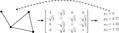
Figure 1: How eigenvalues are obtained from a graph, represented by the solid lines. Spectral graph theory analyzes eigenvalues to deduce properties of the graph, represented by the dashed line.

Two other graph matrices that whose spectra is often studied are the Laplacian matrix $L=D-A$ and normalized Laplacian matrix $\mathcal{L}=D^{-1/2}LD^{-1/2}$, where $D$ denotes the diagonal matrix with the vertex degrees on the diagonal. Unlike the adjacency matrix, both of these matrices are necessarily positive semi-definite, and their spectra characterizes a number of properties which are not captured by adjacency eigenvalues. Due to its intimate connection to random walks and stochastic processes on graphs, the normalized Laplacian matrix is perhaps the most appropriate matrix for characterizing expansion properties of graphs, particularly for irregular graphs. However, we note that if a graph $G$ is $k$-regular (as is the case for a number of supercomputing topologies), then $\mathcal{L}=I-\tfrac{1}{k}A$, from which it is clear that the spectra of all three matrices are related by trivial shifts and scalings by $k$ (and hence functionally the same). We denote the spectrum of the Laplacian matrix $L$ by

$$0=\rho_{1}\leq\rho_{2}\leq\dots\leq\rho_{n},$$

and that of the normalized Laplacian $\mathcal{L}$ by

$$0=\mu_{1}\leq\mu_{2}\leq\dots\leq\mu_{n}\leq 2.$$

We give an example of a graph, its normalized Laplacian, and associated eigenvalues in Figure 1. As we will later see, the eigenvalues $\lambda_{2},\rho_{2}$, and $\mu_{2}$ play a critical role in controlling expansion properties and defining Ramanujan graphs. In particular, the eigenvalue $\rho_{2}$ is called the algebraic connectivity of a graph. Due to its prevalence in the literature (see for instance Brouwer:SpectraGraphs ; Biggs:AGT ; Godsil:AGT ), we will choose to present our results in terms of this spectrum, keeping in mind that if $G$ is $k$-regular, then

$$\rho_{2}=k\cdot\mu_{2}=k-\lambda_{2}.$$

Before proceeding, we describe the spectra of two graphs: the path and the cycle graph. We highlight these graphs as they are frequently elemental to the design of fundamental topologies (e.g. the torus, mesh, and hypercube are all obtained via graph products of cycles or paths). Unsurprisingly, their spectra is highly structured.

• The path of length $n-1$, denoted $P_{n}$, has $n-1$ edges and $n$ vertices, and adjacency spectrum

  $$2\cos\left(\frac{\pi j}{n+1}\right)\mbox{ for }j\in\left\{1,\dots,n\right\}.$$

• If the path of length $n-1$ is modified to add self-loops at each of the endpoints, denoted $P^{\prime}_{n}$, the adjacency spectrum becomes

  $$2\cos\left(\frac{\pi j}{n}\right)\mbox{ for }j\in\left\{0,\dots,n-1\right\}.$$

• The cycle of length $n$, denoted $C_{n}$, has $n$ edges and vertices, and adjacency spectrum

  $$2\cos\left(\frac{2\pi j}{n}\right)\mbox{ for }j\in\left\{0,\dots,n-1\right\}.$$

Finally, we use standard asymptotic notation: a function $f(n)=O(g(n))$ if for all sufficiently large values of $n$ there exists a positive constant $c$ such that $|f(n)|\leq c\cdot|g(n)|$; similarly, we write $f(n)=\Omega(g(n))$ if $g(n)=O(f(n))$, and $f(n)=\Theta(g(n))$ if both $f(n)=O(g(n))$ and $f(n)=\Omega(g(n))$. Lastly, $f(n)=o(g(n))$ if $\lim_{n\to\infty}\frac{f(n)}{g(n)}=0$.

2.1 Network Properties

Graph eigenvalues are deeply related to a number of fundamental network properties. In the case of supercomputing topologies, two such properties linked to communications performance are graph diameter and bisection bandwidth. Diameter (the maximum distance between vertices) is critical for latency, while bisection bandwidth (the minimum number of edges crossing a balanced bipartition of the vertices) measures the networks “bottleneckedness”, impacting all-to-all communication performance.

A plethora of work has shown both of these core network properties to be bounded and thus controlled by graph eigenvalues Chung1989 . In particular, the eigenvalues of interest are the spectral gap, the difference in the largest two adjacency eigenvalues, or the algebraic connectivity, the second smallest Laplacian eigenvalue. For example, Alon and Milman Alon1985 showed that the diameter is at most roughly $C\cdot\log{n}$, where $C$ depends on algebraic connectivity and the maximum degree. More precisely:

Theorem 2.1 (Alon, Milman 1985)

Let $G$ be an $n$-vertex graph with algebraic connectivity $\rho_{2}$ and maximum degree $\Delta$. Then

$$\operatorname{diam}(G)\leq 2\left\lceil\sqrt{\frac{2\Delta}{\rho_{2}}}\log_{2}{n}\right\rceil$$

A lower bound on graph diameter in terms of algebraic connectivity may also be obtained. For example, McKay Mohar:Eigenvalues showed $\mbox{diam}(G)\geq\tfrac{4}{n\rho_{2}}$. In addition to these bounds on the maximum distance between vertices, average distance is upper and lower bounded in terms of algebraic connectivity as well; see Mohar:Eigenvalues . Next, algebraic connectivity provides guarantees on minimum bisection bandwidth, as shown by Fiedler fiedler1973algebraic .

Theorem 2.2 (Fiedler 1975)

Let $G$ be an $n$-vertex graph with algebraic connectivity $\rho_{2}$ and bisection bandwidth $\mbox{BW}(G)$. Then

$$\operatorname{BW}(G)\geq\frac{\rho_{2}n}{4}.$$

By considering Cheeger’s inequality Sokal:gap ; Jerrum:gap one can also obtain upper bounds on the bisection bandwidth in terms of $\rho_{2}$ for regular graphs.

Theorem 2.3

For a connected $k$-regular, $n$-vertex graph $G$ with algebraic connectivity $\rho_{2}$, the bisection bandwidth satisfies

$$\operatorname{BW}(G)\leq\frac{\sqrt{2k\rho_{2}}\cdot kn}{2}.$$

We note that when $\rho_{2}$ is large this upper bound is quite loose. In fact, if $G$ has $m$ edges, an easy application of the first moment method Alon:prob_meth shows the bisection bandwidth is at most $\frac{m}{2}$. Note that if $G$ is $k$-regular and $\rho_{2}$ is asymptotically $k$, then this first moment calculation shows that Theorem 2.2 is essentially tight and the bisection bandwidth is $\frac{kn}{4}\left(1+\it{o}\!\left(1\right)\right)$. Consequently, it can be shown that Ramanujan graphs (defined in Section 3) have nearly optimal bisection bandwidth among all $k$-regular graphs.

Lastly, we note that algebraic connectivity provides bounds on edge and vertex connectivity, the minimum number of edges and vertices that must be deleted in order to disconnect the graph, respectively. In the context of computer interconnection networks, vertex connectivity is often referred to as fault tolerance (e.g., Akers1987a ); more precisely, fault tolerance is defined as one less than vertex connectivity. Denoting vertex and edge connectivity as $\kappa(G),\kappa^{\prime}(G)$ respectively, it is obvious that $\kappa(G)\leq\kappa^{\prime}(G)\leq\Delta(G)$. Fiedler fiedler1973algebraic proved

$$\kappa(G)\geq\rho_{2},$$

hence, larger algebraic connectivity guarantee more robust fault tolerance. For more spectral bounds on vertex and edge connectivity, the reader is referred to Abiad2018 and for further a more complete survey of the relationship between algebraic connectivity and numerous graph invariants, see mohar1991laplacian . Such spectral bounds have practical utility: for a number of graph topologies, exact diameter, bisection bandwidth, etc, may be unknown or difficult to compute and hence eigenvalues may serve as a proxy. In summary, the bounds we’ve reviewed motivate algebraic connectivity as a key parameter of interest intimately related to a plethora of structural properties important to interconnection network design. In the next section, we define graphs with optimal spectral gap, known as Ramanujan graphs, and discuss their expansion properties.

3 Ramanujan Graphs

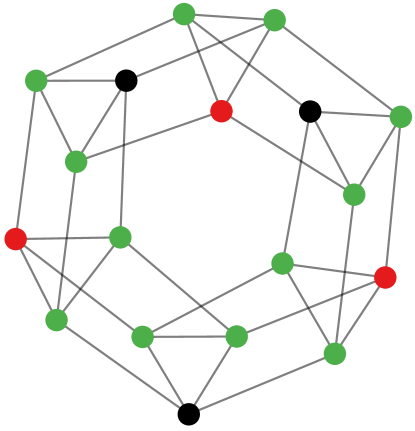
figure*(a)

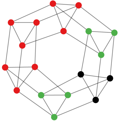
figure*(b)

Figure 2: Examples of a vertex set $X$, in red, with vertex boundary $\partial X$, in green. For (a), the set has vertex isoperimetric ratio 4. For (b), this ratio is $\nicefrac{{2}}{{3}}$, which is the minimum over all subsets whose size doesn’t exceed half the vertices, and thus is the graph’s vertex isoperimetric number.

Ramanujan graphs are regular graphs with nearly optimal expansion properties. Loosely speaking, expansion means that every “not too large” set of vertices has a “not to small” set of neighbors. One way of measuring such expansion is the vertex isoperimetric number of a graph, given by

$$h(G)=\min_{\begin{subarray}{c}X\subseteq V(G)\\ 2|X|\leq|V(G)|\end{subarray}}\frac{|\partial X|}{|X|},$$

where $\partial X$ denotes the neighbors of vertices in $X$ that are not in $X$. We illustrate examples of vertex isoperimetric ratios of sets in Figure 2. This notion of expansion, as well as others such as the edge isoperimetric constant, have been shown to be intimately related to the second largest adjacency eigenvalue of a graph. For example, Tanner Tanner1984 proved a lower bound on $h(G)$ in terms of this eigenvalue $\lambda_{2}$, for a $k$-regular graph; namely,

$$h(G)\geq 1-\frac{k}{2k-2\lambda_{2}}.$$

Conversely, Alon and Milman Alon1985 proved an upper bound on $\lambda_{2}$ in terms of $h(G)$:

$$k-\lambda_{2}\geq\frac{h(G)^{2}}{4+2\cdot h(G)^{2}}.$$

Putting these two bounds together, it is clear that smaller values of $\lambda_{2}$ yield larger values of $h(G)$ and hence better expansion. Other bounds, such as Cheeger’s inequality and Buser’s inequality Buser1982 , similarly tie eigenvalues to other notions of expansion, like the Cheeger constant. Given the breadth of expansion properties reflected through eigenvalues, it is natural to measure expansion directly in terms of the spectra itself. Accordingly, researchers have sought spectral expanders, families of graphs with small $\lambda_{2}$. The most well-known such family are called Ramanujan graphs.

Definition 1

A $k$-regular graph $G$ is called Ramanujan if

$$\lambda(G)\leq 2\sqrt{k-1},$$

where $\lambda(G)$ denotes the largest magnitude adjacency eigenvalue of $G$ not equal to $\pm k$.

Ramanujan graphs are, in a sense, optimal spectral expanders since they achieve the asymptotic theoretical minimum given by Alon-Boppana theorems. The Alon-Boppana theorem Alon:EigenvaluesExpanders ; Nilli:AlonBoppana states that for a $k$-regular graph with second largest (in magnitude) adjacency eigenvalue $\lambda$ and diameter $D$, we have

$$\lambda\geq 2\sqrt{k-1}\left(1-\frac{2}{D}\right)-\frac{2}{D}.$$

As an immediate corollary, if $(G_{i})_{i=1}^{\infty}$ is a family of connected, $k$-regular, $n$-vertex graphs with $n\to\infty$ as $i\to\infty$, then,

$$\liminf_{i\to\infty}\lambda(G_{i})\geq 2\sqrt{k-1}.$$

Hence, we see that Ramanujan graphs attain the theoretical asymptotic optimum spectral expansion. While the Alon-Boppana theorem pertains to regular graphs, variants of the theorem have been proposed for the case of irregular graphs, see chung2016generalized ; Hoory:AlonBoppana ; Young:AlonBoppana .

As a consequence of their optimal spectral expansion, Ramanujan graphs possess beneficial structural properties via the bounds mentioned in Section 2. In particular, not only does the Ramanujan property guarantee at least nearly optimal bisection bandwidth, but also controls the number of edges between any collection of vertices, not just bisections. This stronger property is known as the discrepancy property Chung:spectral . Specifically, using tools of spectral graph theory, if $G$ is an $n$-vertex $k$-regular Ramanujan graph we have that for any two sets of vertices $X$ and $Y$,

$$\left|e(X,Y)-\frac{k}{n}\left|X\right|\left|Y\right|\right|\leq\frac{2\sqrt{k-1}}{n}\sqrt{\left|X\right|(n-\left|X\right|)\left|Y\right|(n-\left|Y\right|)},$$

where $e(X,Y)$ is the number of edges between the sets $X$ and $Y$. Roughly speaking, this says that in any Ramanujan topology the number of edges between two sets scales roughly like the expected number of edges between two sets in a similarly dense random graph. In particular, if a process is active on $\alpha n$ fraction of the nodes of the supercomputing topology, then bisection bandwidth on the active nodes is at least

$$\frac{\alpha kn}{2}\left(\frac{\alpha}{2}-\frac{2\sqrt{k-1}}{k}\left(1-\frac{\alpha}{2}\right)\right)$$

independently of which $\alpha n$ nodes are chosen.

3.1 Ramanujan Constructions

Providing explicit constructions of Ramanujan graphs is challenging. The first explicit constructions of Ramanujan graphs were given by Lubotzky, Phillips, and Sarnak Lubotzky1988 , as well as independently by Margulis margulis1988explicit . Both constructions are Cayley graphs that rely heavily on number-theoretic methods; indeed, the name “Ramanujan graph” was derived due to the application of the Ramanujan–Petersson conjecture from number theory in the aforementioned construction Lubotzky1988 . Below, we briefly describe and compare some of these constructions.

3.1.1 Lubotzky, Phillips, Sarnak Construction

Definition 2 (LPS Graphs)

The LPS graph $X^{p,q}$ is a $(q+1)$-regular Cayley graph, defined for distinct primes $p$ and $q$ such that $p,q\equiv 1\pmod{4}$. Letting $i$ be any integer such that $i^{2}\equiv-1\pmod{p}$, the generating set $S$ of $X^{p,q}$ is given by

$$S=\left\{\begin{bmatrix}\alpha_{0}+i\alpha_{1}&\alpha_{2}+i\alpha_{3}\\ -\alpha_{2}+i\alpha_{3}&\alpha_{0}-i\alpha_{1}\end{bmatrix}\ \middle|\begin{array}[]{l}(\alpha_{0},\alpha_{1},\alpha_{2},\alpha_{3})\mbox{ is a solution of }\alpha_{0}^{2}+\alpha_{1}^{2}+\alpha_{2}^{2}+\alpha_{3}^{2}=q,\\ \alpha_{0}>1\mbox{ is odd, and }\alpha_{1},\alpha_{2},\alpha_{3}\mbox{ are even.}\end{array}\right\},$$

and the group $G$ of $X^{p,q}$ is

$$G=\begin{cases}\mathrm{PSL}(2,\mathbb{F}_{p})&\mbox{ if }\left(\frac{q}{p}\right)=1\vspace{1mm}\\ \mathrm{PGL}(2,\mathbb{F}_{p})&\mbox{ if }\left(\frac{q}{p}\right)=-1\end{cases},$$

where $(\tfrac{q}{p})$ is the Legendre symbol.

We note that in the former case, the Cayley graph of $\mathrm{PSL}(2,\mathbb{F}_{p})$ with generating $S$ has $\tfrac{p(p^{2}-1)}{2}$ vertices and is non-bipartite, while in the latter case, the Cayley graph of $\mathrm{PGL}(2,\mathbb{F}_{p})$ with generating set $S$ is bipartite with $p(p^{2}-1)$ vertices.

Using advanced number-theoretic techniques, Lubotzky, Phillips, Sarnak showed their construction has largest nontrivial adjacency eigenvalue at most $2\sqrt{q}$ and hence is Ramanujan. Additionally, they also showed their construction has other extremal combinatorial properties, such as having girth (i.e. the length of the shortest cycle) of $\Omega(\log_{q}{n})$. From a computational standpoint, the LPS construction allows for explicit querying of vertex-neighborhoods, which is a desirable property for analyzing exponentially large graphs.

The LPS construction may be used to generate infinite families of $(q+1)$-regular Ramanujan graphs; however, only for $q$ prime with $q\equiv 1\pmod{4}$ and $n$ as function of $p$ as given above. That is, despite having outstanding properties, the LPS construction is limited to Ramanujan graphs only of a certain degree – and for each such particular degree, only to a certain number of vertices $n$. In 1994, Morgenstern Morgenstern1994 partially ameliorated this restriction by extending the LPS construction to accommodate any prime power $q$, while showing this extended construction is still Ramanujan and satisfies all other combinatorial properties of the LPS graphs. Nonetheless, this still left open the general case of a given degree $k$ and size $n$.

3.1.2 Marcus, Spielman, Snivrasta construction

In 2013 and 2015, Marcus, Spielman, Snivrasta gave new constructions of Ramanujan graphs using a new technique called the method of interlacing polynomials. Unlike the LPS construction, Marcus, Spielman, and Snivrasta’s first construction Marcus2013 is valid for any given degree $k$, and second construction Marcus2015 is valid both for any $k$ and number of vertices $n$. In both cases, their constructions can only be used to generate bipartite Ramanujan graphs.

While their interlacing family method implicitly suggests an algorithm to find an MSS graph, such an algorithm would require computing partially specified expected characteristic polynomials, for which no known polynomial time algorithms are known Cohen2016 . However, in Cohen2016 , Cohen provided a polynomial time algorithm for computing such polynomials, thereby giving a deterministic algorithm that, for given degree $k$ and even positive integer $n$, returns a bipartite Ramanujan graph, according to the construction given in Marcus2015 , in polynomial time.

3.2 Related work in high-performance computing

Due to the aforementioned relationships between graph expansion and other properties important in network design, many proposed HPC network topologies consider graph expansion implicitly, making a comprehensive review of related work difficult. Before proceeding, we briefly survey related work that explicitly considers Ramanujan graphs or related expanders as network topologies in contexts pertinent to supercomputing. Perhaps most notably, in the context of datacenter architecture design, Valadarsky et al. Valadarsky2016 propose “Xpander”, which utilizes LPS graphs and the theory of graph lifts Bilu2006 . They evaluate Xpander theoretically, via simulation, and using a network emulator, finding that Xpander outperformed traditional data-center designs; see xpanderProjectPage for more. In the early 1990s, Upfal Upfal1992 applied the theory of $(\alpha,\beta,n,d)$-expander graphs to construct so-called “multibutterfly” networks. Later, Brewer, Chong, and Leighton Brewer1994 proposed a hierarchical expander construction, as a means to mitigate wiring complexity; they analyzed the fault tolerance of their so-called “metabutterfly” topology through simulation against the aforementioned multibutterfly. In optical network design, Paturi et al. Paturi1991 proposed using expander graphs to interconnect processors, and subsequently analyze parallel algorithms for sorting, routing, associative memory, and fault-tolerance. Lastly, in the context of sensor networks, Kar and Moura kar2006ramanujan propose using Ramanujan LPS graphs as communication networks supporting distributed decision making, and test their performance on the convergence speed of distributed consensus.

4 Spectral Gap in Supercomputing Topologies

Here, we survey a variety of supercomputing topologies. In addition to giving formal, and in some cases new or generalized, descriptions of the underlying graphs, we focus on analyzing their spectral gap, bisection bandwidth, and diameter. We first consider grid-like and grid variant topologies: the hypercube, generalized grid, torus, butterfly, cube connected cycles and Data Vortex. Then, we consider several miscellaneous topologies: the CLEX, DragonFly, $G$-connected-$H$, and SlimFly topologies. Our results on algebraic connectivity and bisection bandwidth are summarized in Table LABEL:T:boundsBW.

Before proceeding, we first establish a key algebraic tool that we utilize frequently, allowing us to compute subsets of a given graphs spectra through that of a simpler, “reduced” graph.

Lemma 1 (Reduction Lemma)

Let $G$ be a graph and let $\Gamma$ be a subgroup of $\operatorname{Aut}(G)$, the automorphism group of $G$. Let $H$ be a weighted, directed, looped graph with vertex set given by the orbits of $\Gamma$ over $G$ and where the weight of edge from orbit $\sigma$ to orbit $\tau$ is the total weight of an arbitrary vertex $v$ in the orbit $\sigma$ to the orbit $\tau$. The spectrum of $H$ is a subset of the spectrum of $G$. Furthermore, any eigenpair $(\lambda,v)$ of $G$ such that $\lambda$ is not an eigenvalue of $H$ has the property that $v$ sums to zero along orbits of $\Gamma$.

Proof

Let $(\lambda,w)$ be a right eigenpair of $H$. We define the vector $w^{\Gamma}$ as follows; for any vertex $v$ in $G$, define $e_{v}^{T}w^{\Gamma}=e_{\sigma}^{T}w$ where $\sigma$ is the orbit containing $v$. Now let $S$ be the collection of orbits and suppose $v$ is in orbit $\tau$. We then have that

$$e_{v}^{T}A_{G}w^{\Gamma} =\sum_{j}e_{v}^{T}A_{G}e_{j}e_{j}^{T}w^{\Gamma}$$

$$=\sum_{\sigma\in S}\sum_{j\in\sigma}e_{v}^{T}A_{G}e_{j}e_{j}^{T}w^{\Gamma}$$

$$=\sum_{\sigma\in S}\sum_{j\in\sigma}e_{v}^{T}A_{G}e_{j}e_{\sigma}^{T}w$$

$$=\sum_{\sigma\in S}e_{\tau}^{T}A_{H}e_{\sigma}e_{\sigma}^{T}w$$

$$=\lambda e_{\tau}^{T}w$$

$$=\lambda e_{v}^{T}w^{\Gamma}.$$

As $v$ is arbitrary we have that $\lambda$ is also an eigenvalue of $G$.

Now suppose that $(\lambda,v)$ is an eigenpair for $G$ and consider $v^{\Gamma}=\sum_{\sigma\in\Gamma}v_{\sigma}$. Since each $\sigma$ is an automorphism of $G$, $v_{\sigma}$ is also an eigenvector with eigenvalue $\lambda$. Thus $v^{\Gamma}$ is either an eigenvector with eigenvalue $\lambda$ or it is the zero vector. Since $v^{\Gamma}$ is constant over orbits of $\Gamma$, we can form $v^{\Gamma}_{H}$ as the vector of values over orbits. It is clear that $A_{H}v^{\Gamma}_{H}=\lambda v_{H}^{\Gamma}$ and so either $\lambda$ is in the spectrum of $H$ or $v_{H}^{\Gamma}$ is zero and $v$ sums to zero over orbits of $\Gamma$. ∎

We illustrate an application of the Reduction Lemma to a fat tree topology in Figure 3. We note that the Reduction Lemma is almost certainly not new. In fact, it can be viewed as a special case of several other results on describing the interlacing of spectra of a matrix with a quotient matrix, see for instance (Brualdi:GraphsandMatrices, , Chapter 1) and (Brouwer:SpectraGraphs, , Chapter 2).

Figure 3: An application of the Reduction Lemma to the fat tree.

It is worth noting that several of the topologies we will consider have implementations which have minor irregularities in the node radixes. These deviations from regularity have little effect on the true performance of the network and so we will add self-loops as needed to eliminate irregularity and simplify the analysis. This will not change the nature of any of our results as the bisection bandwidth and diameter both are unaffected by arbitrary self-loops.

4.1 Product (Grid-Like) Topologies

For a number of high-dimensional supercomputing topologies, their underlying graphs can be obtained via repeated graph products. Product graphs are highly structured and possess properties which can sometimes be tightly controlled by those of their factor graphs. Below, we briefly describe three such topologies: the hypercube, torus, and generalized grid. These graphs are obtained via a particular graph product called the Cartesian product, denoted $G\mathbin{\text{\scalebox{0.84}{$\square$}}}H$. The graph $G\mathbin{\text{\scalebox{0.84}{$\square$}}}H$ is on vertex set $V(G)\times V(H)$ and is defined by the edge condition: $(u,u^{\prime})$ and $(v,v^{\prime})$ are adjacent if and only if either

• $u=v$ and $\{u^{\prime},v^{\prime}\}\in H$, or

• $u^{\prime}=v^{\prime}$ and $\{u,v\}\in G$.

We note that the adjacency matrix of $G\mathbin{\text{\scalebox{0.84}{$\square$}}}H$, can be written succinctly in terms of those of $G$ and $H$,

$$A_{G\mathbin{\text{\scalebox{0.84}{$\square$}}}H}=A_{G}\otimes I+I\otimes A_{H},$$

where $I$ denotes the identity matrix and $\otimes$ denotes Kronecker product. Using the above characterization, it is easy to show that the adjacency (or Laplacian) eigenvalues of $A_{G\mathbin{\text{\scalebox{0.84}{$\square$}}}H}$ consists of $\lambda(G)_{i}+\lambda(H)_{j}$ over all $1\leq i\leq|V(G)|$ and $1\leq j\leq|V(H)|$; hence the $d$-fold Cartesian product eigenvalues consists of all possible $d$-sums of the factor graph eigenvalues. In particular, the algebraic connectivity of $G\mathbin{\text{\scalebox{0.84}{$\square$}}}H$ is the minimum of the algebraic connectivity of $G$ and the algebraic connectivity of $H$.

Definition 3 (Hypercube, $Q_{d}$)

The $d$-dimensional hypercube, $Q_{d}$, is on $n=2^{d}$ vertices, defined by the $d$-fold Cartesian product $P_{2}\mathbin{\text{\scalebox{0.84}{$\square$}}}\dots\mathbin{\text{\scalebox{0.84}{$\square$}}}P_{2}$, where $P_{2}$ is the path with 1 edge.

It is well-known that $Q_{d}$ has algebraic connectivity of $2$ and bisection bandwidth $2^{d-1}=n/2$. The hypercube is a special case of the generalized grid graph, defined below.

Definition 4 (Generalized Grid, $G_{k_{1},\dots,k_{d}}$)

The $d$-dimensional, generalized grid the $d$-fold Cartesian product $P_{k_{1}}\mathbin{\text{\scalebox{0.84}{$\square$}}}\cdots\mathbin{\text{\scalebox{0.84}{$\square$}}}P_{k_{d}}$, where $P_{k_{i}}$ is the path of length ${k_{i}-1}$.

We note that taking $d=2$, $k_{1}=m$, and $k_{2}=n$ yields what is sometimes simply referred to as a grid graph, or $m\times n$ lattice, while taking $k_{1}=\dots=k_{d}=2$ yields $Q_{d}$. Using the aforementioned fact relating the Cartesian product eigenvalues to those of the factor graphs, it is easy to see the algebraic connectivity of $G_{k_{1},\dots,k_{d}}$ is $2-2\cos(\pi/\max\{k_{1},\dots,k_{d}\})$. Finally, we define the discrete torus topology, which is given by the cartesian product of cycles.

Definition 5 (Torus, $C^{d}_{k}$)

The discrete torus $C^{d}_{k}$ is the $d$-fold graph box product of a $k$-cycle, i.e. $C_{k}\mathbin{\text{\scalebox{0.84}{$\square$}}}\dots\mathbin{\text{\scalebox{0.84}{$\square$}}}C_{k}$. This graph is regular on $n=k^{d}$ vertices, and has degree $2d$.

It is not difficult to show the algebraic connectivity of the torus $C^{d}_{k}$ is $2(1-\cos(\nicefrac{{2\pi}}{{k}}))$.

4.2 Grid Variants

The collection of topologies we consider in this section are closely related to topologies formed from the product operation, but with minor twists or modifications. Oftentimes these toplogies start from some grid-like layout and permute the connections or add small substructures to achieve desired properties.

4.2.1 Butterfly

One of the more well known grid variants is the Butterfly topology Leighton:Intro . In its most simple form the Butterfly topology consists of a sereis of shuffling layers based on the binary representation of the node names. More concretely, there are $p\log_{2}(p)$ switches arranged in a $\log_{2}(p)$-by-$p$ array of $p$ switches in one of $\log_{2}(p)$ ranks. For each rank, each of the $p$ switches is connected to two switches in the previous rank and two switches in the next rank. The nodes in rank $i$ and position $j$ are connected to the switch $j$ and switch $m$ in rank $i-1$, where $m$ is formed by flipping the $i^{\textrm{th}}$ bit in binary representation of $j$. It is also connected to switch $j$ and $m^{\prime}$ in rank $i+1$, where $m^{\prime}$ is formed by switching the $(i+1)^{\textrm{st}}$ bit in $j$. The Butterfly topology has diameter $\log_{2}(p)$ and bisection width $\nicefrac{{p}}{{2}}$

Definition 6 (Butterfly, $\operatorname{Butterfly}(k,s)$)

The $k$-ary, $s$-fly butterfly network where there are $s$-layers of switches, and each switch has $k$ “forward” connections. More concretely, the switches can be indexed by elements of $[s]\times[k]^{s}$. The “forward” connections from $(i,(a_{1},\ldots,a_{s}))$ to $(i+1,(a_{1}^{\prime},\ldots,a_{s}^{\prime}))$ are formed by keeping all but the $i^{\textrm{th}}$ component of $a$ fixed, i.e. $a_{j}=a_{j}^{\prime}$ if $j\neq i$. Depending on the application, the $s$ layers can either be connected linearly (no connection from layer $s$ to layer $1$), or cyclically (connection from layer $s$ to layer $1$). For convenience, we will restrict ourselves to the cyclic arrangement.

It is straightforward to see that these networks have a diameter of $s$ by considering two elements in the same layer, $(i,\mathbf{a})$ and $(i,\mathbf{b})$, where no coordinate of $\mathbf{a}$ and $\mathbf{b}$ agree.

Proposition 1

Let $G$ be a $k$-ary, $s$-fly Butterfly network. The bisection bandwidth of $G$ is at most $\frac{(k+1)k^{s}}{2}$ and the algebraic connectivity is at most $2k-2k\cos\left(\frac{2\pi}{s}\right)$.

Proof

To upper bound the bisection bandwidth we first consider the case where $k$ is even and define $X=\left[\frac{k}{2}\right]\times[k]^{s-1}$. The bipartition we consider is then $([s]\times X,[s]\times\overline{X})$. In order for $(s,x)\in[s]\times X$ and $(s,x^{\prime})\in[s]\times\overline{X}$ to be adjacent, it must be the case that $\left\{s,s^{\prime}\right\}=\left\{1,2\right\}$ and $x$ and $x^{\prime}$ differ only in the first coordinate. This gives that $e([s]\times X,[s]\times\overline{X})=2\left(\frac{k}{2}\right)^{2}k^{s-1}=\frac{k^{s+1}}{2}$.

When $k$ is odd the we construct a slightly more complicated partition. In particular, for $0\leq i\leq s-1$ define $X_{i}=\left\{\frac{k+1}{2}\right\}^{i}\times\left[\frac{k-1}{2}\right]\times[k]^{s-1-i}$ and let $X=\bigcup_{i}X_{i}$. Note that

$$\left|X\right|=\sum_{i=0}^{s-1}\left|X_{i}\right|=\frac{k-1}{2}\sum_{i=0}^{s-1}k^{s-1-i}=\frac{k-1}{2}\frac{k^{s}-1}{k-1}=\frac{k^{s}-1}{2}.$$

In particular $([s]\times X,[s]\times\overline{X})$ is a bipartition of the vertex set of the $k$-ary, $s$-fly Butterfly network. Now to evaluate the bisection bandwidth we wish to count pairs $(u,v)\in X_{i}\times\overline{X}$ such that $u$ and $v$ differ in precisely one component. If we fix some $x_{i}\in X_{i}$, then for all $1\leq j\leq i+1$, modifying the $j^{\textrm{th}}$ component to be in $\frac{k+3}{2},\ldots,k$ yields such a pair. We note that modifying any entry $j>i+1$ will preserve membership in $X_{i}$. Thus the only remaining case to consider is when index $(i+1)$ is modified to have value $\frac{k+1}{2}$. This takes us outside the set $X$ if and only if $x_{i}\not\in\left\{\frac{k+1}{2}\right\}^{i}\times\left[\frac{k-1}{2}\right]\times\left\{\frac{k+1}{2}\right\}^{j}\times\left[\frac{k-1}{2}\right]\times[k]^{s-2-i-j}$ for some $0\leq j\leq s-2-i$. As there are $\frac{k-1}{2}\frac{k^{s-i-1}+1}{2}$ such terms $x_{i}$, this gives that the total number of pairs $(u,v)\in X_{i}\times\overline{X}$ which differ by exactly one component is given by

$$\left(\frac{k-1}{2}\right)k^{s-i-1}(i+1)\left(\frac{k-1}{2}\right)+\left(\frac{k-1}{2}\right)\left(\frac{k^{s-i-1}+1}{2}\right)=\frac{\left(k-1\right)\left((i+1)k^{s-i}-ik^{s-i-1}+1\right)}{4}.$$

Thus the bisection bandwidth is at most

$$\sum_{i=0}^{s-1}2\frac{\left(k-1\right)\left((i+1)k^{s-i}-ik^{s-i-1}+1\right)}{4} =\frac{s(k-1)}{2}+\frac{k-1}{2}\sum_{i=0}^{s-1}(i+1)k^{s-i}-ik^{s-i-1}$$

$$=\frac{s(k-1)}{2}+\frac{k-1}{2}\left(k^{s}+2\frac{k^{s}-k}{k-1}-(s-1)\right)$$

$$=\frac{k-1}{2}+\frac{k^{s+1}-k^{s}}{2}+k^{s}-k$$

$$=\frac{k^{s+1}+k^{s}-k-1}{2}.$$

To upper bound the algebraic connectivity, we note that there is an automorphism group of the Butterfly topology in which the orbits are given by the layers. Thus, by applying the reduction lemma to this automorphism group we get an $s$-cycle with edge multiplicity $k$. The bound on the algebraic connectivity then follows immediately. ∎

4.2.2 Data Vortex

The Data Vortex topology was designed as a “streaming” topology with the idea that all of the data is constantly in motion (i.e., it is never buffered) and the data swirls from processors in the outer ring of the vortex towards the processors on the inside of the topology Hawkins2007 ; Shacham2005 . This streaming methodology has allowed the Data Vortex topology to handle the transmission of high-volumes of data without suffering from signficant congestion related performance degradation (see Gioiosa2017 ; Gioiosa2016 ; Iliadis2007 ; Yang2002 for a more in-depth discussion of the performance benefits of the Data Vortex topology.). Formally, the topology is defined a series concentric cylinders with “angular” transitions between them. Within the cylinders there is a switching topology reminiscent of the layers of the 2-ary Butterfly topology. More concretely, we have:

Definition 7 (Data Vortex, $\operatorname{DataVortex}(A,C)$)

The Data Vortex topology with parameters $A,C$ is a graph with vertex set $\mathbb{Z}_{A}\times\mathbb{Z}_{C}\times\mathbb{Z}_{2}^{C-1}$, and edge set given by:

1. for all $(a,c,h)\in\mathbb{Z}_{A}\times\mathbb{Z}_{C}\times\mathbb{Z}_{2}^{C-1}$ there is an edge to $(a+1,c+1,h)$,

2. for all $(a,c,h)\in\mathbb{Z}_{A}\times\left(\mathbb{Z}_{C}-\left\{0\right\}\right)\times\mathbb{Z}_{2}^{C-1}$ there is an edge to $(a+1,c,h+e_{c})$ where $e_{c}$ denotes the unit vector for the $c^{\textrm{th}}$ component of $\mathbb{Z}_{2}^{C-1}$, and

3. for all $(a,c,h)\in\mathbb{Z}_{A}\times\left\{0\right\}\times\mathbb{Z}_{2}^{C-1}$ there is an edge to $(a+1,c,h)=(a+1,0,h)$.

Although the Data Vortex is designed as a streaming topology (and is in particular, indirect), we will consider it as a direct topology in which each node denotes a compute node.

Proposition 2

The algebraic connectivity of the Data Vortex topology with $A$ angles and height $H$ is at most $\min\left\{2-2\cos\left(\frac{\pi}{C}\right),2-2\cos\left(\frac{2\pi}{A}\right)\right\}=\mathcal{O}\!\left(\frac{1}{\max\left\{A^{2},(C-1)^{2}\right\}}\right)$. Furthermore, the bisection bandwidth is at most $A2^{C-2}$.

Proof

We begin by first noting that the vertices in the outer and inner ring of the Data Vortex have degree 3, so we will consider the topology formed by adding a self loop to each of these vertices. Alternatively, we could add an edge between corresponding vertices in the inner and outer ring by observing that in typical use cases these vertices are connected to a common system, forming the “input” and “output” ports of the system. However, this modification results in essentially the same asymptotic behavior, so we choose the self-loop modification as it is requires no assumptions about how the Data Vortex interacts with the processing layer of the overall system.

We first consider the bisection bandwidth by separating the vertices based on height, specifically partitioning into vertices of height $1,\ldots,2^{C-2}$, and those of height $2^{C-2}+1,\ldots,2^{C-1}$. Clearly this is a bisection. As no edge between concentric rings changes height, it suffices to consider only those edges internal to a ring. However, as only one ring flips the leading bit of the height vector, this gives that the bisection bandwidth is at most $A2^{C-2}$.

In order to bound the algebraic connectivity, we will apply the reduction lemma. Specifically we consider the automorphism group generated by the bit-flip operations on the height. As these act uniformly on the height the edges between successive rings are clearly preserved. Further, as the bit-wise differences are preserved by the bit-flip operations, this preserves edges on each ring. Under this automorphism group, the Data Vortex topology reduces to $C_{A}\mathbin{\text{\scalebox{0.84}{$\square$}}}P^{\prime}_{C}$ where $P^{\prime}_{k}$ is the $k$-vertex path with loops at each end. The result bounding the algebraic connectivity follows immediately. ∎

4.2.3 Cube Connected Cycles

Loosely speaking, the Cube Connected Cycles (CCC) graph consists of a hypercube in which each vertex has been replaced by a cycle. Preparata and Vuillemin Preparata1981 proposed the Cube-Connected Cycles as a versatile network topology for connecting processors in a parallel computer, which emulates the the robust connectivity properties of the hypercube, but (due to the cycle modification) only requires three connections per processor. They conclude that “by combining the principles of parallelism and pipelining, the CCC can emulate the cube connected machine and shuffle-exchange network with no significant degradation in performance.”

As suggested in Riess2012 , CCC graph is a special case of a more general graph construction in which an arbitrary graph is connected in a hypercube structure. More precisely:

Definition 8 (Cube Connected Cycles, $\operatorname{CCC}(d)$)

The $d$-dimensional cube-connected graph of a given graph $G$, denoted $\mathrm{CC}(G,d)$, has vertex set $V(G)\times\{0,1\}^{d}$ and edge condition $(v_{i},x)\sim(v_{j},y)$ if and only if

• $v_{i}\sim v_{j}$ in $G$, or

• $v_{i}=v_{j}$ and the hamming distance between $x$ and $y$ is 1.

Taking $G=C_{d}$ yields the well-known Cube-Connected Cycles graph. Riess, Strehl, and Wanka proved the following result, which relates the characteristic polynomial of $\mathrm{CC}(G)$ to those of loop-weighted variants of $G$:

Theorem 4.1 (Riess, Strehl, Wanka Riess2012 )

Let $G$ be an $d$-vertex graph. For $\mathbf{s}=(s_{1},\dots,s_{d})\in\{-1,1\}^{d}$, let $G[\mathbf{s}]$ denote the graph obtained from $G$ by adding a loop of weight $s_{i}$ to each vertex $i$. Then

$$\chi(\mathrm{CC}(G,d))=\prod_{\mathbf{s}\in\{-1,1\}^{d}}\chi(G[\mathbf{s}]),$$

where $\chi(G)$ denotes the characteristic polynomial of the adjacency matrix of $G$.

As an immediate consequence, we have that the spectral set of $\mathrm{CC}(G,d)$ is the union of the spectral sets of $G[\mathbf{s}]$ over all $\mathbf{s}\in\{-1,1\}^{d}$. Using their result, we can derive good estimates of the spectral expansion of the CCC. To do so, we first prove the following lemma.

Lemma 2

Let $G$ be a connected, $n$-vertex graph. The second largest adjacency eigenvalue of $\mathrm{CC}(G,d)$ is the maximum eigenvalue of $G[\mathbf{s}^{*}]$, where $\mathbf{s}^{*}=(s_{1},\dots,s_{d})\in\{-1,1\}^{d}$ is such that for some fixed $j\in[n]$, $s_{j}=-1$ and for all other $i\not=j$, $s_{i}=1$.

In the proof of Lemma 2, we will use the following basic fact:

Fact 1

Let $G$ be a connected, $n$-vertex graph. Let $\mathbf{r},\mathbf{t}\in\{-1,1\}^{d}$, $\mathbf{r}\not=\mathbf{t}$, be such that $\mathbf{r}$ agrees with $\mathbf{t}$ on any $i\in[n]$ where $t_{i}=1$, and let $i_{1},\dots,i_{k}\in[n]$ denote indices on which they differ, i.e. where $t_{i_{j}}=-1$ and $r_{i_{j}}=1$ for $j\in[k]$. Then the largest adjacency eigenvalue of $G[\mathbf{r}]$ is strictly greater than that of $G[\mathbf{t}]$.

Proof

Let $A$ and $A^{\prime}$ denote the adjacency matrices of $G[\mathbf{r}]$ and $G[\mathbf{t}]$, respectively, and let $\mathbf{x}=(x_{1},\dots,x_{n})$ denote the normalized, dominant eigenvector of $A^{\prime}+I$, whose entries are all positive by the Perron-Frobenius theorem. By definition, we have $\mathbf{x}^{T}(A+I)\mathbf{x}\ -\ \mathbf{x}^{T}(A^{\prime}+I)\mathbf{x}=2\sum_{j=1}^{k}x_{i_{j}}^{2}>0.$ ∎

Proof (Proof of Claim 2)

From Theorem 4.1 and Fact 1, we have that the largest adjacency eigenvalue of $\mathrm{CC}(G,d)$ is that of $G[\mathbf{1}_{d}]$, and furthermore that if $\mathbf{1}_{d}\not=\mathbf{t}\in\{-1,1\}^{d}$ does not satisfy the property in the claim, then there exists some $\mathbf{s}$ that does, which we denote $\mathbf{s}^{*}$, such that $\lambda_{1}(G[\mathbf{t}])<\lambda_{1}(G[\mathbf{s}^{*}])$. So, let $G$ and $G^{\prime}$ denote $G[\mathbf{1}_{d}]$ and $G[\mathbf{s}^{*}]$, respectively, on vertex set $\{v_{1},\dots,v_{n}\}$, where $v_{j}$ denotes the vertex in $G[\mathbf{s^{*}}]$ with a loop of weight $-1$. Labeling the adjacency eigenvalues $\lambda_{1}\geq\dots\geq\lambda_{n}$, all that remains to show is that

$$\lambda_{2}(G)<\lambda_{1}(G^{\prime}).$$ (1)

By Cauchy’s interlacing theorem, if we delete $v_{j}$ from $G$ and $G^{\prime}$, we have

$$\lambda_{2}(G) \leq\lambda_{1}(G\setminus v_{j})\leq\lambda_{1}(G),$$

$$\lambda_{2}(G^{\prime}) \leq\lambda_{1}(G^{\prime}\setminus v_{j})\leq\lambda_{1}(G^{\prime}).$$

But since $G\setminus v_{j}=G^{\prime}\setminus v_{j}$, combining the above inequalities yields

$$\lambda_{2}(G)\leq\lambda_{\max}(G\setminus v_{j})\leq\lambda_{1}(G^{\prime}).$$

To see the inequality in $(\ref{eqn:strictInq})$ is strict, assume for contradiction that $\lambda_{1}(G^{\prime}\setminus v_{j})=\lambda_{1}(G^{\prime})$. Then if $\mathbf{x}=(x_{1},\dots,x_{j},\dots,x_{n})$ denotes the dominant eigenvector of $A^{\prime}$ associated with $\lambda_{1}$, this implies if we set $x_{j}=0$, the vector $(x_{1},\dots,0,\dots,x_{n})$ is still an eigenvector of $G^{\prime}$ associated with $\lambda_{1}$. But applying the Perron-Frobenius theorem to $A^{\prime}+I$ yields that the dominant eigenvector of $A^{\prime}+I$ (and hence that of $A^{\prime}$) is unique and has all entries positive, which is a contradiction. ∎

Using Lemma 2, we have:

Proposition 3

The algebraic connectivity of the $d$-dimensional, cube-connected cycles is at most on the order of $2\left(1-\cos\left(\frac{\pi}{d+2}\right)\right)$.

Proof

By Lemma 2, it suffices to consider the largest adjacency eigenvalue $\lambda_{1}$ of the $d$-cycle with one loop of weight $-1$ on one vertex, and loops of weight 1 on other vertices. Letting $A^{\prime}$ denote this graphs adjacency matrix, a routine calculation shows that for ${\bf x}=(x_{1},\dots,x_{n})$ defined by $x_{i}=\sin\left(\frac{\pi i}{d+2}\right)$,

$$\lambda_{1}(A^{\prime})\geq\frac{\langle\mathbf{x},A^{\prime}\mathbf{x}\rangle}{\langle\mathbf{x},\mathbf{x}\rangle} =2\cos\left(\frac{\pi}{d+2}\right)+1+\frac{\sin^{2}(\tfrac{\pi}{d+2})\left(2\cos(\tfrac{\pi}{d+2})-2\right)}{\tfrac{d+1}{2}+\cos(\tfrac{2\pi}{d+2})}.$$

We note that above expression is strictly larger than the second largest adjacency eigenvalue of the d-cycle with all loops of weight 1, for $d\geq 2$.

∎

It is worth mentioning that the Cube Connected Graphs are really a specific instance of a more general technique of constructing supercomputing topologies, which we refer to as $G$-connected-$H$. As the generic $G$-connected-$H$ topologies are not grid-like topologies we will defer their discussion to Section 4.3.2.

4.3 Miscellaneous

In this section we consider a few topologies that do not (necessarily) have a strong grid structure. Typically these topologies have some sort of recursive or multi-layer structure in order to attempt to combine “good” properties of several types of graphs.

4.3.1 CLEX

“Clique-Expander” (CLEX) is a new supercomputing topology recently introduced by Lenzen and Wattenhofer Lenzen2016 . The CLEX construction is recursive, starting with a specified number of cliques that are sparsely interconnected. According to the authors, the CLEX design is motivated by a desire to “localize the issue of an efficient communication network to much smaller systems which may reside on a single multi-core board”. CLEX is touted to have superior point-to-point communication properties, particularly when compared with toroidal topologies; nonetheless, the Lenzen and Wattenhofer acknowledge “the price we pay for these properties are [high] node degrees”.

In this section, we will define the CLEX topology, and prove new bounds on the diameter, algebraic connectivity, and bisection bandwidth. As the authors of CLEX note that that “the high connectivity of a CLEX system could be considered an abstraction that can be replaced by any efficient local communication scheme within the cliques”, we generalize our spectral analysis of CLEX accordingly. In particular, our analysis allows one to replace the cliques of the CLEX construction with other graphs. We first begin by defining the CLEX graph, as given in Lenzen2016 .

Definition 9 (CLEX, $C(k,\ell)$)

For given positive integers $k$ and $\ell$, a CLEX digraph, denoted $C(k,\ell)$, is on $n=k^{\ell}$ vertices with $\ell$ “levels”, and is defined recursively. The base case is $C(k,1)=K_{k}$, the complete graph on $k$ vertices. The vertex set of $C(k,\ell+1)$ is the $(\ell+1)$-fold cartesian product of $V(K_{k})$. The edge set of $C(k,\ell+1)$ consists of all edges from $k$ copies of $C(k,\ell)$, with additional directed edges between these copies. Note the last entry in each vertex identifies which “copy” of $C(k,\ell)$ that vertex belongs to. The additional edges between these copies of $C(k,\ell)$ are given by the set:

$$\{((v_{1},\ldots,v_{l},i),\hskip 2.84526pt(v_{1},\ldots,v_{\ell-1},j,v_{\ell})):i,j\in[k]\}.$$

With regard to the diameter of CLEX, the authors in Lenzen2016 give an upper bound of $C(k,\ell)$ as $2^{\ell}-1$. We claim that the diameter is bounded by $\ell$.

Proposition 4

The diameter of the CLEX graph $C(k,\ell)$ is at most $\ell$. Furthermore, this bound is tight.

Proof

We construct a walk of length $\ell$ between two arbitrary vertices of $C(k,l)$, $(v_{1},\ldots,v_{l})$ and $(w_{1},\ldots,w_{\ell})$ as follows:

$$(v_{1},\ldots,v_{\ell}),(w_{\ell},v_{2},\ldots,v_{\ell}),(w_{1},w_{l},v_{3},\ldots,v_{\ell}),(w_{1},w_{2},w_{l},v_{4},\dots,v_{\ell}),\dots,(w_{1},\ldots,w_{\ell-1},w_{\ell}).$$

Furthermore, this bound can seen to be tight by considering the path between $(i,i,\ldots,i)$ and $(j,j,\ldots,j)$ for any $i\neq j$. Specifically, although each edge can modify up to two positions in the vector describing the vertex, it can change the count of any particular symbol in the string by at most one. ∎

The rest of our analysis will consider the CLEX digraph as an undirected multi-graph (potentially with loops). Specifically, for every directed edge $(i,j)$ in the CLEX digraph we will have an undirected edge $\left\{i,j\right\}$ and thus the total degree of any vertex does not change. As our analysis only relies minimally on the structure of $K_{k}$, we will consider a generalized version of CLEX, denoted $C(G,\ell)$ where $G$ is a $t$-regular, connected graph on $k$ vertices. We note that both the regularity and connectivity conditions can be relaxed at various points in the following analysis, however we make both assumptions for simplicity of presentation.

We first note that even when $G\neq K_{k}$, the arguments regarding the diameter follow exactly after accounting for the diameter of $G$ and potentially directed nature of $G$.

Lemma 3

Let $G$ be a $k$-vertex graph, then

$$C(G,\ell)=G\otimes I_{k^{\ell-1}}+\sum_{j=0}^{\ell-2}I_{k^{j}}\otimes M\otimes I_{k^{\ell-2-j}},$$

where $M\in\mathbb{Z}^{k^{2}\times k^{2}}$ is given by

$$M_{(i,j),(a,b)}=\begin{cases}2&i=b,j=a\\ 1&i=b,j\neq a\\ 1&i\neq b,j=a\\ 0&\textrm{otherwise}.\end{cases}$$

Proof

The generic formula will follow immediately from the inductive characterization of the CLEX graphs. We note that the edges of $C(G,\ell+1)$ can be partitioned in two sets, those that come from $C(G,\ell)$ and the cross edges “between” copies of $C(G,\ell)$. Letting $C^{G}_{\ell}$ be the adjacency matrix for $C(G,\ell)$, the edge coming from the copies of $C(G,\ell)$ can be described by $C_{\ell}^{G}\otimes I_{k}$. Now note that an edge is added between $(v_{1},\ldots,v_{\ell-1},v_{\ell},v_{\ell+1})$ and $(w_{1},\ldots,w_{\ell-1},w_{\ell},w_{\ell+1})$ precisely when $v_{i}=w_{i}$ for $1\leq i\leq\ell_{i}$ and $v_{\ell+1}=w_{\ell}$ or $w_{\ell+1}=v_{\ell}$. Thus the cross edges are given by $I_{k^{\ell-1}}\otimes M$ and we have that

$$C^{G}_{\ell+1}=C^{G}_{\ell}\otimes I_{k}+I_{k^{\ell-1}}\otimes M.$$

The non-inductive formula follows immediately from this relationship. ∎

Lemma 4

Let $M\in\mathbb{Z}^{k^{2}\times k^{2}}$ be defined by

$$M_{(i,j),(a,b)}=\begin{cases}2&i=b,j=a\\ 1&i=b,j\neq a\\ 1&i\neq b,j=a\\ 0&\textrm{otherwise}.\end{cases}$$

We then have that $\operatorname{spec}\!\left(M\right)$ is the multiset $\left\{2k,k^{(k-1)},(-k)^{(k-1)},0^{(k-1)^{2}}\right\}$.

Proof

Let $\left\{e_{i}\right\}$ be the standard basis vectors for $\mathbb{R}^{k}$ and let $\mathbbm{1}$ be the all ones vector in $\mathbb{R}^{k}$. We first note that

$$M=\sum_{i=1}^{k}\left(\mathbbm{1}\otimes e_{i}\right)\left(e_{i}\otimes\mathbbm{1}\right)^{T}+\left(e_{i}\otimes\mathbbm{1}\right)\left(\mathbbm{1}\otimes e_{i}\right)^{T}.$$

It is easy to see at this point that $\mathbbm{1}\otimes\mathbbm{1}$ is an eigenvector of $M$ with eigenvalue $2k$. Furthermore, we can see that the non-trivial eigenvectors must lie in $\operatorname{span}\!\left\{\left\{\mathbbm{1}\otimes e_{i}\right\}_{i}\cup\left\{e_{i}\otimes\mathbbm{1}\right\}_{i}\right\}$, as a $2k-1$ dimensional subspace of $\mathbb{R}^{k^{2}}$.

Now consider

$$M\left(e_{j}\otimes\mathbbm{1}\right) =\sum_{i=1}^{k}\left(\left(\mathbbm{1}\otimes e_{i}\right)\left(e_{i}\otimes\mathbbm{1}\right)^{T}+\left(e_{i}\otimes\mathbbm{1}\right)\left(\mathbbm{1}\otimes e_{i}\right)^{T}\right)\left(e_{j}\otimes\mathbbm{1}\right)$$

$$=\sum_{i=1}^{k}\left(\mathbbm{1}\otimes e_{i}\right)\left(e_{i}\otimes\mathbbm{1}\right)^{T}\left(e_{j}\otimes\mathbbm{1}\right)+\left(e_{i}\otimes\mathbbm{1}\right)\left(\mathbbm{1}\otimes e_{i}\right)^{T}\left(e_{j}\otimes\mathbbm{1}\right)$$

$$=k\left(\mathbbm{1}\otimes e_{j}\right)+\sum_{i=1}^{k}e_{i}\otimes\mathbbm{1}$$

$$=k\left(\mathbbm{1}\otimes e_{j}\right)+\mathbbm{1}\otimes\mathbbm{1}.$$

Similarly, we have that $M\left(\mathbbm{1}\otimes e_{j}\right)=k\left(e_{j}\otimes\mathbbm{1}\right)+\mathbbm{1}\otimes\mathbbm{1}$. From this it easy to see that

$$M\left(e_{j}\otimes\mathbbm{1}-\mathbbm{1}\otimes e_{j}\right)=-k\left(e_{j}\otimes\mathbbm{1}-\mathbbm{1}\otimes e_{j}\right),$$

for all $j$. Noting that $\sum_{j}\left(e_{j}\otimes\mathbbm{1}-\mathbbm{1}\otimes e_{j}\right)=0$, we have that this yields a $k-1$-dimensional eigenspace associated with the eigenvalue $-k$. Finally, we note that $M\left(e_{j}\otimes\mathbbm{1}+\mathbbm{1}\otimes e_{j}-\frac{2}{k}\mathbbm{1}\otimes\mathbbm{1}\right)=k\left(e_{j}\otimes\mathbbm{1}+\mathbbm{1}\times e_{j}-\frac{2}{k}\mathbbm{1}\otimes\mathbbm{1}\right)$, we similarly observe a $k-1$ dimensional eigenspace associated with the eigenvalue $k$. As the dimension of the non-trivial eigenspaces is at most $2k-1$, this provides a complete characterization of the spectrum. ∎

Proposition 5

Let $G$ be a $t$-regular, connected graph on $k$ vertices. The algebraic connectivity of $C(G,\ell)$ is at most $t+3k-1$.

Proof

First we note that since $G$ is $t$-regular, $C(G,\ell)$ is $t+2k\left(\ell-1\right)$ regular. Now let $(\lambda,v)$ be the eigenpair associated with the second largest eigenspace of $G$ such that $\left\|v\right\|=1$ and let $w=v\otimes\left(\frac{1}{\sqrt{k}}\mathbbm{1}\right)^{\otimes\ell-1}$. Since $G$ is $t$-regular, we have that $\left<v,\mathbbm{1}\right>=0$ and thus $\left<w,\mathbbm{1}^{\otimes\ell}\right>=0$. Furthermore, since $\left\|v\right\|=1$ and $\left\|\frac{1}{\sqrt{k}}\mathbbm{1}\right\|=1$, we have that $\left\|w\right\|=1$. Thus $w^{T}Mw$ is a lower bound on the second largest eigenvalue of $C(G,\ell)$. We now note that

$$w^{T}Mw =w^{T}G\otimes I_{k^{\ell-1}}w+\sum_{i=0}^{\ell-2}w^{T}I_{i}\otimes M\otimes I_{\ell-2-i}w$$

$$=\lambda+(v\otimes\mathbbm{1})^{T}M(v\otimes M)+\sum_{i=1}^{\ell-2}2k$$

$$\geq\lambda-k+2k(\ell-2)$$

$$=-1-k+2k(\ell-2).$$

Thus the spectral gap is at most $t+2k(\ell-1)-\left(-1-k+2k(\ell-2)\right)=t+3k+1$. ∎

Proposition 6

Let $G$ be a $t$-regular connected graph. If $\ell\geq 3$, the bisection bandwidth of $C(G,\ell)$ is at most $k^{\ell+1}$.

Proof

We may assume without loss of generality that the vertices of $G$ are given by $[k]=\left\{1,\ldots,k\right\}$ and thus the vertex set of $C(G,\ell)$ is given by $[k]^{\ell}$. In order to upper bound the bisection bandwidth we will provide two explicit partitions of the vertex set, one for the case when $k$ is even and a modification construction for when $k$ is odd. To that end, define $A$ to be the set of odd integers in $[k]$ if $k$ is even, and in $[k-1]$ if $k$ is even. Similarly define $A^{\prime}$ to be the set of even integers in $[k]$. We note that if $k$ is even then $[k]$ is a disjoint union of $A$ and $A^{\prime}$, while if $k$ is odd $[k]$ is a disjoint union of $A$, $A^{\prime}$, and $\left\{k\right\}$.

We first consider the case where $k$ is even and define the sets $X=[k]^{\ell-2}\times\left(A\times A^{\prime}\cup A^{\prime}\times A\right)$ and $\overline{X}=[k]^{\ell-2}\times\left(A\times A\cup A^{\prime}\times A^{\prime}\right)$. Since $\left|A\right|=\left|A^{\prime}\right|$ and $[k]$ is a disjoint union of $A$ and $A^{\prime}$, it is clear that $(X,\overline{X})$ is a bisection of the $C(G,\ell)$.

Now let $A_{\ell}$ be the adjacency matrix of $C(G,\ell)$ and let $\mathbbm{1}_{X}$ (respectively $\mathbbm{1}_{\overline{X}}$) be the indicator vector for the set $X$ (respectively $\overline{X}$). By definition

$$\operatorname{BW}\left(C(G,\ell)\right)=\mathbbm{1}_{X}^{T}A_{\ell}\mathbbm{1}_{\overline{X}}=\mathbbm{1}^{T}_{X}\left(G\otimes I_{k^{\ell-1}}+\sum_{j=0}^{\ell-2}I_{k^{j}}\otimes M\otimes I_{k^{\ell-2-j}}\right)\mathbbm{1}_{\overline{X}}.$$

Noting that for any set $S$, we have that$\mathbbm{1}_{S}^{T}I_{\left|S\right|}\mathbbm{1}_{\overline{S}}=0$ as $S$ and $\overline{S}$ are disjoint, this can be simplified to

$$\operatorname{BW}\left(C(G,\ell)\right) =\mathbbm{1}_{X}^{T}\left(I_{k^{\ell-3}}\otimes M\otimes I_{k}+I_{k^{\ell-2}}\otimes M\right)\mathbbm{1}_{\overline{X}}$$

$$=k^{\ell-3}\left(\mathbbm{1}_{[k]\times A\times A^{\prime}}+\mathbbm{1}_{[k]\times A^{\prime}\times A}\right)^{T}\left(M\otimes I_{k}+I_{k}\otimes M\right)\left(\mathbbm{1}_{[k]\times A\times A}+\mathbbm{1}_{[k]\times A^{\prime}\times A^{\prime}}\right)$$

$$=k^{\ell-3}\left(2\frac{k}{2}\mathbbm{1}_{[k]\times A}^{T}M\mathbbm{1}_{[k]\times A^{\prime}}+4k\mathbbm{1}_{A\times A^{\prime}}M\mathbbm{1}_{A\times A}\right),$$

where the last line comes from the symmetry of $A$ and $A^{\prime}$ and the symmetry of $M$ in terms of the Kronecker product. Substituting in the defintion for $M$ we get

$$\left(\mathbbm{1}\otimes\mathbbm{1}_{A}\right)^{T}M\left(\mathbbm{1}\otimes\mathbbm{1}_{A^{\prime}}\right) =\sum_{i=1}^{k}\left(\mathbbm{1}\otimes\mathbbm{1}_{A}\right)^{T}\left((e_{i}\otimes\mathbbm{1})(\mathbbm{1}\otimes e_{i})^{T}+(\mathbbm{1}\otimes e_{i})(e_{i}\otimes\mathbbm{1})^{T}\right)\left(\mathbbm{1}\otimes\mathbbm{1}_{A^{\prime}}\right)$$

$$=\sum_{i=1}^{k}\left|A\right|k\left(e_{i}^{T}\mathbbm{1}_{A^{\prime}}\right)+k\left(e_{i}^{T}\mathbbm{1}_{A}\right)\left|A^{\prime}\right|$$

$$=2k\left|A\right|\left|A^{\prime}\right|$$

$$=\frac{k^{3}}{2}$$

and

$$\left(\mathbbm{1}_{A}\otimes\mathbbm{1}_{A^{\prime}}\right)^{T}M\left(\mathbbm{1}_{A}\otimes\mathbbm{1}_{A}\right) =\sum_{i=1}^{k}\left(\mathbbm{1}_{A}\otimes\mathbbm{1}_{A^{\prime}}\right)\left((e_{i}\otimes\mathbbm{1})(\mathbbm{1}\otimes e_{i})^{T}+(\mathbbm{1}\otimes e_{i})(e_{i}\otimes\mathbbm{1})^{T}\right)\left(\mathbbm{1}_{A}\otimes\mathbbm{1}_{A}\right)$$

$$=\sum_{i=1}^{k}\left(\mathbbm{1}_{A}^{T}e_{i}\right)\frac{k}{2}\frac{k}{2}\left(e_{i}^{T}\mathbbm{1}_{A}\right)+\frac{k}{2}\left(\mathbbm{1}_{A^{\prime}}^{T}e_{i}\right)\left(e_{i}^{T}\mathbbm{1}_{A}\right)\frac{k}{2}$$

$$=\frac{k^{3}}{8}.$$

Thus we have that if $k$ is even, the bisection bandwidth is $k^{\ell+1}$.

We now turn to the case where $k$ is odd. Because of the parity issues in this case, it will be convient to define the bipartition inductively. To that end, let $(B,\overline{B})$ be a bipartition of $C(G,\ell-2)$ which witnesses the bandwidth such that $\left|B\right|+1=\left|\overline{B}\right|$. Now define the sets

$$Y =[k]^{\ell-2}\times\left((A\times A^{\prime})\cup(A^{\prime}\times A)\cup(\left\{k\right\}\times[k-1])\right)\cup\left(B\times\left\{k\right\}\times\left\{k\right\}\right)$$

$$\overline{Y} =[k]^{\ell-2}\times\left((A\times A)\cup(A^{\prime}\times A^{\prime})\cup([k-1]\times\left\{k\right\})\right)\cup\left(\overline{B}\times\left\{k\right\}\times\left\{k\right\}\right).$$

It is clear that since $\left|A\right|=\left|A^{\prime}\right|$ and $\left|\left|B\right|-\left|B^{\prime}\right|\right|=1$, that $(Y,\overline{Y})$ is a bipartition of $[k]^{\ell}$. Abusing notation slightly, and we denote the set $[k]^{\ell-2}\times\left((A\times A^{\prime})\cup(A^{\prime}\times A)\right)$ by $X$ and the set $[k]^{\ell-2}\times\left((A\times A)\cup(A^{\prime}\times A^{\prime})\right)$ as $\overline{X}$. If we again let $A_{\ell}$ denote the adjacency matrix of $C(G,\ell)$, we have that

$$\mathbbm{1}_{X}^{T}A_{\ell}\mathbbm{1}_{\overline{X}}=(k-1)^{3}k^{\ell-2}$$

by similar arguments as above. Additionally, we note that we have that

$$\left(\mathbbm{1}\otimes\mathbbm{1}_{A}\right)^{T}M\left(\mathbbm{1}\otimes\mathbbm{1}_{[k-1]}\right) =k(k-1)^{2}$$

$$\left(\mathbbm{1}\otimes\mathbbm{1}_{A}\right)^{T}M\left(\mathbbm{1}\otimes e_{k}\right) =k(k-1)$$

$$\left(\mathbbm{1}\otimes\mathbbm{1}_{[k-1]}\right)^{T}M\left(\mathbbm{1}\otimes e_{k}\right) =2k(k-1)$$

$$\left(\mathbbm{1}_{A}\otimes\mathbbm{1}_{A^{\prime}}\right)^{T}M\left(e_{k}\otimes\mathbbm{1}_{[k-1]}\right) =\frac{(k-1)^{2}}{4}$$

$$\left(\mathbbm{1}_{A}\otimes\mathbbm{1}_{A^{\prime}}\right)^{T}M\left(e_{k}\otimes e_{k}\right) =0$$

$$\left(\mathbbm{1}_{[k-1]}\otimes e_{k}\right)^{T}M\left(e_{k}\otimes e_{k}\right) =k-1.$$

$$\left(\mathbbm{1}_{[k-1]}\otimes e_{k}\right)^{T}M\left(e_{k}\otimes\mathbbm{1}_{[k-1]}\right) =k(k-1)$$

Putting these calculations together, we get that the bandwidth of the partition $(Y,\overline{Y})$ is

$$(k-1)k^{\ell}+\mathbbm{1}_{[k]^{\ell-2}\times[k-1]}^{T}\left(I_{k^{\ell-3}}\otimes M\right)\mathbbm{1}_{B\times\left\{k\right\}}+\mathbbm{1}_{B\times\left\{k\right\}\times\left\{k\right\}}^{T}A_{\ell}\mathbbm{1}_{B\times\left\{k\right\}\times\left\{k\right\}}.$$

Observing that $A_{\ell}=A_{\ell-2}\otimes I_{k^{2}}+I_{k^{\ell-3}}\otimes M\otimes I_{k}+I_{k^{\ell-2}}\otimes M$, it is easy to see that

$$\mathbbm{1}_{B\times\left\{k\right\}\times\left\{k\right\}}^{T}A_{\ell}\mathbbm{1}_{\overline{B}\times\left\{k\right\}\times\left\{k\right\}}=\operatorname{BW}(C(G,\ell-2))+\mathbbm{1}_{B\times\left\{k\right\}}^{T}\left(I_{k^{\ell-3}}\otimes M\right)\mathbbm{1}_{\overline{B}\times\left\{k\right\}}$$

Now we note that terms involving $\mathbbm{1}_{B\times\left\{k\right\}}$ sum to

$$\left(\mathbbm{1}_{[k]^{\ell-1}}-\mathbbm{1}_{B\times\left\{k\right\}}\right)^{T}\left(I_{k^{\ell-3}}\otimes M\right)\mathbbm{1}_{B\times\left\{k\right\}} =\mathbbm{1}_{[k]^{\ell-1}}\left(I_{k^{\ell-3}}\otimes M\right)\mathbbm{1}_{B\times\left\{k\right\}}-\mathbbm{1}_{B\times\left\{k\right\}}^{T}\left(I_{k^{\ell-3}}\otimes M\right)\mathbbm{1}_{B\times\left\{k\right\}}$$

$$=2k\left|B\right|-\mathbbm{1}_{B\times\left\{k\right\}}^{T}\left(I_{k^{\ell-3}}\otimes M\right)\mathbbm{1}_{B\times\left\{k\right\}}$$

$$\leq k\left(k^{\ell-2}-1\right)$$

Thus we have that

$$\operatorname{BW}\left(C(G,\ell)\right) \leq(k-1)k^{\ell}+k^{\ell-1}-k+\operatorname{BW}\left(C(G,\ell-2)\right)$$

$$=k^{\ell+1}-k^{\ell}+k^{\ell-1}-k+BW\left(C(G,\ell-2)\right).$$

Now, as $\operatorname{BW}\left(C(G,1)\right)\leq k^{2}$ and $\operatorname{BW}\left(C(G,2)\right)\leq k^{3}$, it is easy to see that by induction $\operatorname{BW}\left(C(G,\ell)\right)\leq k^{\ell+1}$. ∎

4.3.2 $G$-connected-$H$

The $G$-connected-$H$ construction generalizes several different constructions, such as the Peterson Torus and Dragonfly topologies discussed in this section as well as the Cube Connected Cycle topology discussed in Section 4.2.3. To see this, we first formally define what we mean by a $G$-connected-$H$ topology.

Definition 10 ($k$-fold $G$-connected-$H$, $G\textrm{\reflectbox{$\rightsquigarrow$}}_{k}H$)

A $k$-fold $G$-connected-$H$ topology, $\mathcal{G}=G\textrm{\reflectbox{$\rightsquigarrow$}}_{k}H$, is constructed from a $d$-regular $G$ and a $r$-regular $td$-vertex graph $H$. The vertex set of $\mathcal{G}$ is $V_{G}\times V_{H}$ and $G[\left\{g\right\}\times V_{H}]$ is isomorphic to $H$ for all vertices $g\in V_{G}$. The remaining edges form a $k$-regular graph on $V_{G}\times V_{H}$ satisfying that

$$e\!\left(\left\{v\right\}\times V_{H},\left\{v^{\prime}\right\}\times V_{H}\right)=\begin{cases}kt&\left\{v,v^{\prime}\right\}\in E_{G}\\ 0&\textrm{otherwise}\end{cases}.$$

When $k=1$ will surpress the subscript and simply write $G\textrm{\reflectbox{$\rightsquigarrow$}}H$.

Oftentimes, $G$ is a Cayley graph and so the $k$-regular graph on $V_{G}\times V_{H}$ can be defined by a mapping from the generators of $G$ to ordered pairs in $V_{H}^{2}$. For example, we denote by $Q_{k}$ the $k$-dimensional hypercube, we can view the Cube Connecte Cycle topology of Section 4.2.3 as a $1$-fold $Q_{k}$-connected-$C_{k}$. More concretely, we note that $Q_{k}$ can be represented as the Cayley graph on $\mathbb{Z}_{2}^{k}$ generated by the standard basis vectors, $\left\{e_{1},\ldots,e_{k}\right\}$. Since the generators of $Q_{k}$ have order two, the matching edges can be formed by associating each generator with a fixed vertex of $C_{k}$.

This viewpoint can be extend to more complicated topologies, such as the Peterson Torus JungHyun2008 .

Definition 11 (Peterson Torus, $\operatorname{PT}(a,b)$)

Let $a,b\geq 2$ such that at least one of $a$ or $b$ is odd. Define the vertex set of the Peterson Torus Topology, $\operatorname{PT}(a,b)$, as the set of ordered triples $(x,y,p)$ where $0\leq x<a$, $0\leq y<b$, and $0\leq p<10$. Fixing the labels of the Peterson graph as given in Figure 4a the edge relationship is defined as:

• internal edge $\left(x,y,p\right)$ is adjacent to $\left(x,y,q\right)$ if $p$ and $q$ are adjacent in the Petersen graph.

• longitudinal edge $\left(x,y,6\right)$ is adjacent to $\left(x,y+1,9\right)$.

• latitudinal edge $\left(x,y,1\right)$ is adjacent to $\left(x+1,y,4\right)$.

• diagonal edge $\left(x,y,2\right)$ is adjacent to $\left(x+1,y+1,3\right)$.

• reverse diagonal edge $\left(x,y,7\right)$ is adjacent to $\left(x-1,y+1,8\right)$.

• diameter edge $\left(x,y,0\right)$ is adjacent to $\left(x+\left\lfloor\nicefrac{{a}}{{2}}\right\rfloor,y+\left\lfloor\nicefrac{{b}}{{2}}\right\rfloor,5\right)$.

This can be seen as a $1$-fold $G$-connected-$H$ graph where $G$ being the Cayley graph on $Z_{a}\times\mathbb{Z}_{b}$ with generator set $\left\{\pm(0,1),\pm(1,0),\pm(1,1),\pm(-1,1),\pm(\left\lfloor\nicefrac{{a}}{{2}}\right\rfloor,\left\lfloor\nicefrac{{b}}{{2}}\right\rfloor)\right\}$ and $H$ being the Peterson graph. We note that the condition that one of $a$ or $b$ is odd, is simply to ensure that the generator $(\left\lfloor\nicefrac{{a}}{{2}}\right\rfloor,\left\lfloor\nicefrac{{b}}{{2}}\right\rfloor)$ is not it’s own inverse and so $G$ has degree 10. By allowing multiple edges in $G$, this restriction can be eliminated.

(a) Peterson Graph

(b) Reduced $\operatorname{PT}(a,b)$

Figure 4: Peterson Graph and the Peterson Graph with the Symmetric Function induced by the Peterson Torus

We first consider the bisection bandwidth of $G\textrm{\reflectbox{$\rightsquigarrow$}}_{k}H$. As this will depend explicitly on the number of nodes and edges in $H$, it is helpful to recall some standard notation first. Following the notation of West West:GraphTheory , the number of nodes in a network $G$ will be denoted by $\left|G\right|$ and the number of edges will be denoted $\left\|G\right\|$.

Proposition 7

Let $\mathcal{G}=G\textrm{\reflectbox{$\rightsquigarrow$}}_{k}H$, then the bisection bandwidth of $\mathcal{G}$ is at most $\frac{\left|G\right|\left|H\right|}{2\left\|G\right\|}k\operatorname{BW}(G)+\operatorname{BW}(H)$.

Proof

We note that if $\left|G\right|$ is even, then the bipartition of $G$ yielding $\operatorname{BW}(G)$, lifts naturally to a bipartition of $G\textrm{\reflectbox{$\rightsquigarrow$}}_{k}H$. As each edge in $G$ is represented by $\frac{\left|G\right|\left|H\right|}{2\left\|G\right\|}k$ edges in $G\textrm{\reflectbox{$\rightsquigarrow$}}_{k}H$, this gives an upper bound of $\frac{\left|G\right|\left|H\right|}{2\left\|G\right\|}k\operatorname{BW}(G)$. If instead, $\left|G\right|$ is odd, the natural lift of the minimal bipartition doesn’t yield a bipartition of $G\textrm{\reflectbox{$\rightsquigarrow$}}_{k}H$. However, this can be corrected by splitting one of the copies of $H$, yielding the extra $\operatorname{BW}(H)$ term. ∎

We now turn the algebraic connectivity of $G\textrm{\reflectbox{$\rightsquigarrow$}}_{k}H$. Because of the general structure of the matching edges and the potentially unstructured nature of $G$ and $H$, the reduction lemma can not be applied in general to $G$-connected-$H$ graphs. However, there is still a natural symmetry formed by the $G$-connected-$H$ structure, specifically the identification of vertices by common $G$ labels or common $H$ labels. However, because of the lack of automorphism structure we must turn to eigenvalue interlacing results such as the following by Haemmers.

Lemma 5

(Brualdi:GraphsandMatrices, , Corollary 1.8) Let $A$ be an $n\times n$ real-symmetric matrix with eigenvalues $\lambda_{1}\geq\lambda_{2}\geq\cdots\geq\lambda_{n}$. Let $\alpha_{1},\ldots,\alpha_{m}$ be a partition of the integers $\left\{1,2,\ldots,n\right\}$ into $m$ nonempty consecutive sets of integers, where $\left|\alpha_{i}\right|=n_{i}$. Let $A_{ij}$ be the submatrix of $A$ defined by the entries whose row is in $\alpha_{i}$ and column is in $\alpha_{j}$. Define $B$ as the $m\times m$ real symmetric matrix with

$$b_{ij}=\frac{\mathbbm{1}_{n_{i}}^{T}A_{ij}\mathbbm{1}_{n_{j}}}{n_{i}}.$$

The eigenvalues of $B$ interlace the eigenvalues of $A$, in particular, $\lambda_{2}(B)\leq\lambda_{2}$.

Proposition 8

Let $G$ be a connected $d$-regular graph and let $H$ be a connected $r$-regular, $td$-vertex graph, and let $\mathcal{G}=G\textrm{\reflectbox{$\rightsquigarrow$}}_{k}H$ be a $k$-fold $G$-connected-$H$ graph. Let $\lambda_{2}$ be the second largest eigenvalue of $G$, then the algebraic connectivity of $\mathcal{G}$ is at most $k-\frac{k\lambda_{2}}{d}$.

Proof

Let $A$ be the adjacency matrix of $\mathcal{G}=G\textrm{\reflectbox{$\rightsquigarrow$}}_{k}H$. We will proceed to show that $\lambda_{2}(\mathcal{G})\geq\frac{1}{d}\lambda_{2}+r$ and then the desired result follows immediately from the $(r+k)$-regularity of $\mathcal{G}$. To this end we will apply Lemma 5 to the partion of the vertices given by $\left\{\left\{v\right\}\times V_{H}\right\}_{v\in V_{G}}$. Abusing notation, for any $v,v^{\prime}\in V_{G}$ we will denote by $A_{vv^{\prime}}$ the submatrix induced by the rows $\left\{v\right\}\times V_{H}$ and columns $\left\{v^{\prime}\right\}\times V_{H}$. Noting that $\left|\left\{v\right\}\times V_{H}\right|=td$ for all $v\in V_{G}$, we have that

$$\mathbbm{1}_{td}^{T}A_{vv^{\prime}}\mathbbm{1}_{td}=\begin{cases}rtd&v=v^{\prime}\\ tk&\left\{v,v^{\prime}\right\}\in E_{G}\\ 0&\left\{v,v^{\prime}\right\}\not\in E_{G}\end{cases}$$

and thus $B=rI+\frac{k}{d}A_{G}$ where $A_{G}$ is the adjacency matrix of the graph $G$. The interlacing of the eigenvalues of $B$ and $\mathcal{G}$ provides the result immediately. ∎

The strong dependence on the spectrum of $G$ is unsurprising as the $G$-connected-$H$ graphs implicitly inherent the connectivity structure of $G$, while increasing the relative degrees in a way that doesn’t improve the spectral behavior of $G$. In particular, we note that another way of deriving Lemma 8 is to apply the Raleigh-Ritz formulation of $\lambda_{2}(\mathcal{G})$ and use the vector $\frac{1}{\sqrt{td}}\mathbbm{1}\otimes w_{2}$ where $(\lambda_{2},w_{2})$ is the second largest eigenpair of $A_{G}$.

It is natural to consider the implications of Lemma 5 when partitioning on the $H$-coordinate instead of the $G$-coordinate. Unfortunately, because of the unstructured nature of the $k$-regular graph relatively little can be said. However, if the graph $G$ is Cayley graph and the matching edges are tied to the generator set then the automorphisms of $G$ (specifically, those that follow from vertex transitivity of Cayley graphs) imply that there is an automorphism of $G\textrm{\reflectbox{$\rightsquigarrow$}}H$ such that the orbits are given by $V_{G}\times\left\{h\right\}$ for $h\in V_{H}$. Then the Reduction Lemma yields that there is multi-graph whose spectrum is a subset of the spectrum of $G\textrm{\reflectbox{$\rightsquigarrow$}}_{k}H$. Specifically, taking the graph $H$ plus a $k$-regular graph (allowing self-loops) coming from the structure of the $k$-regular graph in $G\textrm{\reflectbox{$\rightsquigarrow$}}_{k}H$. As an example, the Peterson Torus can be reduced with the reduction lemma to the graph illustrated with in Figure 4b with the red edges corresponding to the matching edges. Computing the algebraic connectivity of the reduced graph yields that the $\rho_{2}$ for the Peterson torus is at most 2. While this is small, it can be reduced further by applying Proposition 8.

Corollary 1

Let $a\geq b\geq 2$ such that at least one of $a$ or $b$ is odd. The algebraic connectivity of $\operatorname{PT}(a,b)$ is at most $\frac{4-3\cos\left(\frac{4\pi}{a}\right)-\cos\left(\frac{2\pi}{a}\right)}{5}$ and the bisection bandwidth is at most $6b+ab+5$.

Proof

By Proposition 8 to bound the algebraic connectivity it suffices to find the second largest eigenvalue of the Cayley graph $G$ on the group $\Gamma=\mathbb{Z}_{a}\times\mathbb{Z}_{b}$ generated by

$$S=\left\{\pm(1,0),\pm(0,1),\pm(1,1),\pm(1,-1),\pm\left(\left\lfloor\nicefrac{{a}}{{2}}\right\rfloor,\left\lfloor\nicefrac{{b}}{{2}}\right\rfloor\right)\right\}.$$

Let $\chi\colon\Gamma\rightarrow\mathbb{C}^{\left|\Gamma\right|}$ be the character table for $\Gamma$. We recall that the spectrum of $G$ is explicitly given by the multiset

$$\left\{\sum_{s\in S}\chi_{g}(s)\mid g\in\Gamma\right\},$$

see for instance Brouwer:SpectraGraphs . As $\Gamma$ is the product of two cyclic groups, it is straightforward to explicitly determine the character table and get that the spectrum is given by the multiset

$$\left\{\sum_{(s,t)\in S}e^{\frac{2\pi ix}{a}s}e^{\frac{2\pi iy}{b}t}\mid(x,y)\in\mathbb{Z}_{a}\times Z_{b}\right\}.$$

In particular, this gives that $\lambda_{2}$ for $G$ is given by

$$2\max_{(x,y)\not\equiv(0,0)}\cos\!\left(\frac{2\pi x}{a}\right)+\cos\!\left(\frac{2\pi y}{b}\right)+2\cos\left(\frac{2\pi x}{a}\right)\cos\!\left(\frac{2\pi y}{b}\right)+\cos\left(\frac{2\pi\left\lfloor\nicefrac{{a}}{{2}}\right\rfloor x}{a}+\frac{2\pi\left\lfloor\nicefrac{{b}}{{2}}\right\rfloor y}{b}\right).$$

It is relatively straightforward to see that the maximum is achieved when $(x,y)=(2,0)$, yielding that $\lambda_{2}$ is at least

$$2+6\cos\left(\frac{4\pi}{a}\right)+2\cos\left(\frac{4\pi\left\lfloor\frac{a}{2}\right\rfloor}{a}\right)\geq 2+6\cos\left(\frac{4\pi}{a}\right)+2\cos\left(\frac{2\pi}{a}\right).$$

The upper bound on the bisection bandwidth will follow from Lemma 7. Specifically, as the Peterson torus is a $G\textrm{\reflectbox{$\rightsquigarrow$}}H$ with $G$ being the Cayley graph on $\mathbb{Z}_{a}\times\mathbb{Z}_{b}$ with generators $S$ and $H$ the Peterson graph, the bisection bandwidth is upper bounded by $\operatorname{BW}(G)+\operatorname{BW}(H)$. As the girth of the Peterson graph is 5, any collection of 5 vertices induces at most 5 edges. Thus there are at least 5 edges crossing the cut, and this lower bound is achieved exactly by taking any of the 5-cycles in the Peterson graph.

For the bisection bandwidth of the graph on $\mathbb{Z}_{a}\times\mathbb{Z}_{b}$, we will denote the vertices by $[a]\times[b]$. If $a$ is even, then the set $T=[\frac{a}{2}]\times[b]$ induces a bipartition with $6b+ab$ edges crossing the cut, that is, the edges corresponding to elements $\left\{\frac{a}{2}\right\}\times[b]$ and the generators $\left\{(1,-1),(1,0),(11)\right\}$, the edges corresponding to the elements $\left\{1\right\}\times[b]$ and the generators $\left\{(-1,-1),(-1,0),(-1,1)\right\}$, and the edges corresponding to an arbitrary vertex of $T$ and the generators $\left\{\left(\left\lfloor\frac{a}{2}\right\rfloor,\left\lfloor\frac{b}{2}\right\rfloor\right),\left(-\left\lfloor\frac{a}{2}\right\rfloor,-\left\lfloor\frac{b}{2}\right\rfloor\right)\right\}$. In the case that $a$ is odd, we consider the set $[\left\lfloor\frac{a}{2}\right\rfloor]\times[b]\cup\left\{\left\lceil\frac{a}{2}\right\rceil\right\}\times[\left\lfloor\frac{b}{2}\right\rfloor]$ and in a similar manner get that there are $6b+2\left\lfloor\frac{ab}{2}\right\rfloor$ edges crossing the cut, completing the proof. ∎

4.3.3 DragonFly

As we will see, the DragonFly topology will end up being a specific class of $G$-connected-$H$ topologies and can be understood in terms of the results of Section 4.3.2, however, due to their recent importance in “readily” available supercomputing topologies Cray:Slingshot ; Cray:XC we address them separately in this section. The motivating idea behind the DragonFly topology is to maximize the performance of a supercomputing topology while minimizing the overall cost of the system. To that end, Kim, Dally, Scott, and Abts designed the DragonFly topology around a two-level hierarchy Kim2008 . The top level network employs an optical network to communicate over long distances (i.e. across the physical layout of the supercomputer), while the second layer employs an electrical network to communicate short distances (i.e. intrarack communication) and reduce the overall cost. While the specifications of Kim, et al. allow for arbitrary topologies for both the optical and electrical portions of the topology, the typically implementation uses a fully-connected optical network combined with some other network for the electrical network, oftentimes either fully-connected or a Butterfly variant. For example, the Cray Slingshot interconnect (which is being used for NSERC’s Perlmutter system) uses 64 port switches to build a DragonFly topology based on all-to-all connections for both the optical and electrical networks.

Definition 12 (DragonFly, $\operatorname{DragonFly}(H)$)

If $H$ is an $n$-vertex, $r$-regular graph, then the DragonFly topology with parameter $H$ consists of $n+1$ copies of $H$ together with a matching such that each edge goes between distinct copies of $H$. Alternatively, $\operatorname{DragonFly}(H)$ may be thought of as a $1$-fold $K_{n}\textrm{\reflectbox{$\rightsquigarrow$}}H$.

We note that since the DragonFly topology can be represented as $G\textrm{\reflectbox{$\rightsquigarrow$}}H$ topology we immediately have bounds on the algebraic connectivity and bisection bandwidth.

Corollary 2

Let $H$ be a connected graph and let $D$ be the DragonFly topology generated by $H$. The algebraic connectivity of $D$ is at most $1+\frac{\left|H\right|}{2\left\|H\right\|}$ and the bisection bandwidth is at most

$$\left(\frac{\left|H\right|+1}{2}\right)^{2}+\operatorname{BW}(H).$$

Proof

Noting that $D=K_{\left|H\right|+1}\textrm{\reflectbox{$\rightsquigarrow$}}H$ and the second largest adjacency eigenvalue of the complete graph is $-1$, the bound on the algebraic connectivity follows immediately from Proposition 8. To provide the upper bound on the bisection bandwidth, consider a equipartition of the $\left|H\right|+1$ copies of $H$. If $\left|H\right|$ is odd, then the only edges crossing the partition are “matching” or “optical” edges and there are $\left(\frac{\left|H\right|+1}{2}\right)^{2}$ of them. However, if $\left|H\right|$ is even, then one of the copies of $H$ must also be partitioned yielding

$$\left(\frac{\left|H\right|}{2}\right)^{2}+\frac{\left|H\right|}{2}+\operatorname{BW}(H)\leq\left(\frac{\left|H\right|+1}{2}\right)^{2}+\operatorname{BW}(H)$$

edges crossing the partition. ∎

4.3.4 SlimFly

In Besta:SlimFly , Besta and Hoefler suggested that it would be advantageous to consider topologies that have close to the maximum number of nodes for a given radix and diameter. The upper bound on the number of nodes of a $k$-regular graph of diameter $d$ is given by $1+k\sum_{i=0}^{d-1}(k-1)^{i}$ and is referred to as the Moore bound. The class of graphs exactly achieving this bound, known as Moore graphs, has been extensively studied and shown to have significant limitation on both the radix and size, see Miller:MooreSurvey .

In this context, Besta and Hoefler propose the SlimFly topology based on the construction of McKay, Miller, and Širán McKay:MMS which is close to achieving the Moore bound. These SlimFly topologies have a single parameter $q$, which is a prime power such that $q\equiv 1\pmod{4}$ and results in a topology on $2q^{2}$ nodes with degree $\frac{3q-1}{2}$.

Definition 13 (SlimFly, $\operatorname{SlimFly}(q)$)

Let $\zeta$ be a primitive $q^{\textrm{th}}$-root of unity over the Galois field $\mathbb{F}_{q}$. The vertices are then elements of $\left\{0,1\right\}\times\mathbb{F}_{q}\times\mathbb{F}_{q}$. The edge set is broken into three sets:

1. $\left\{(0,x,y),(0,x,y^{\prime})\right\}$ where $y-y^{\prime}=\zeta^{i}$ and $i\equiv 0\pmod{2}$,

2. $\left\{(1,m,c),(1,m,c^{\prime})\right\}$ where $c-c^{\prime}=\zeta^{j}$ and $j\equiv 1\pmod{2}$, and

3. $\left\{(0,x,y),(1,m,c)\right\}$ where $y=mx+c$.

Proposition 9

Let $q$ be a prime-power such that $q\equiv 1\pmod{4}$. The algebraic connectivity of the SlimFly topology with parameter $q$ is $q$.

Proof

In order to bound the algebraic connectivity, we will use the Reduction Lemma. To that end, let $\zeta$ be a primitive root of the Galois field $\mathbb{F}_{q}$ and define $\gamma_{\zeta}$ by $(0,x,y)\mapsto(0,x,y+\zeta)$ and $(1,m,c)\mapsto(1,m,c+\zeta)$. It is easy to see that this is an automorphism of the SlimFly topology and that the orbits of the group generated by this automorphism are given by $\left\{0\right\}\times\left\{x\right\}\times\mathbb{F}_{q}$ and $\left\{1\right\}\times\left\{m\right\}\times\mathbb{F}_{q}$ for $x,m\in\mathbb{F}_{q}$. As an arbitrary element $(0,x,y)\in\left\{0\right\}\times\mathbb{F}_{q}\times\mathbb{F}_{q}$, has precisely one neighbor in the orbit $\left\{1\right\}\times\left\{m\right\}\times\mathbb{F}_{q}$ for any $m\in\mathbb{F}_{q}$, namely $(1,m,y-mx)$, we have that the reduction graph $H$ is a complete bipartite graph $K_{q,q}$ with $\frac{q-1}{2}$ self-loops at every vertex. As the algebraic connectivity of this graph is $q$, by the Reduction Lemma we have that the algebraic connectivity of the is at most $q$.

Now we will show that the algebraic connectivity is exactly $q$. To this end, recall that the eigenspace associated to any eigenvalue that is not present in the spectrum of the reduced graph has the property that the entries sum to zeros over all of the orbits. That is, if $v$ is such an eigenvector and $\mathbbm{1}_{\sigma}$ is the indicator function for the orbit $\sigma$, then $v^{T}\mathbbm{1}_{\sigma}=0$. Furthermore, since the orbits of the automorphism are Cayley graphs on $\mathbb{F}_{q}$, the eigenvectors can be expressed in terms of the characters of $\left(\mathbb{F}_{q},+\right)$. Additionally, the eigenvalues associated to $\chi_{f}$ are given by the character sums over the generators. Specifically, the eigenvalue associated to the non-trivial character $\chi$ on the Cayley graph generated by $\zeta^{2j}$ is $\mu=\sum_{j=1}^{\nicefrac{{q-1}}{{2}}}\chi(\zeta^{2j})$, while the eigenvalue associated to $\chi$ on the Cayley graph generated by $\zeta^{2j-1}$ is $\sum_{j=1}^{\nicefrac{{q-1}}{{2}}}\chi(\zeta^{2j-1})=-1-\mu$. Thus let $\left\{\chi_{f}\right\}_{f=1}^{q-1}$ be the set of non-trivial characters of $\left(\mathbb{F}_{q},+\right)$. The eigenvector $v$ can then be expressed as

$$\sum_{i\in\left\{0,1\right\}}\sum_{x\in\mathbb{F}_{q}}\sum_{f\in[q-1]}\frac{a_{i,x,f}}{\sqrt{q}}e_{i}\otimes e_{x}\otimes\chi_{f}$$

where $\sum_{i,x,f}\alpha_{i,x,f}^{2}=1$

Now letting $A$ be the adjacency matrix of the SlimFly topology, we consider the quadratic form $\overline{v}^{T}Av$ in three parts. The portion corresponding to edges induced by $\left\{0\right\}\times\mathbb{F}_{q}\times\mathbb{F}_{q}$, the portion corresponding to edges induced by $\left\{1\right\}\times\mathbb{F}_{q}\times\mathbb{F}_{q}$, and the portion corresponding to edges between these two sets. It is easy to see that the contribution of the edges internal to these two sets are given by $\sum_{f=1}^{q-1}\sum_{x\in\mathbb{F}_{q}}\overline{\alpha_{0,x,f}}\alpha_{0,f,x}\mu_{f}$ and $\sum_{f=1}^{q-1}\sum_{m\in\mathbb{F}_{q}}\overline{\alpha_{0,m,f}}\alpha_{1,m,f}(-1-\mu_{f})$, respectively. Recalling the edges between the two sets are governed by the relationship $y=mx+c$ for $(x,y),(m,c)\in\mathbb{F}_{q}^{2}$, we have that the contribution of those edges to the quadratic form is

$$\sum_{f,g=1}^{q-1}\sum_{(x,y)\in\mathbb{F}_{q}^{2}}\sum_{(m,c)\in\mathbb{F}_{q}^{2}}\frac{\overline{\alpha_{0,x,f}}\alpha_{1,m,g}}{q}\overline{\chi_{f}(y)}\chi_{g}(c)\mathbbm{1}_{y=mx+c}+\frac{\alpha_{0,x,f}\overline{\alpha_{1,m,g}}}{q}\chi_{f}(y)\overline{\chi_{g}(c)}\mathbbm{1}_{y=mx+c}.$$

Now we note that the non-zero entries in the sum occur when $c=y-mx$. Furthermore, $\chi_{g}$ is a homomorphism into $(\mathbb{C},\times)$ so $\chi_{g}(y-mx)=\chi_{g}(y)\chi_{g}(-mx)$. By additionally recalling that $\left\{\chi_{f}\right\}_{f=1}^{q-1}$ is an orthogonal basis, this sum simplifies to

$$\sum_{f=1}^{q-1}\sum_{x\in\mathbb{F}_{q}}\sum_{y\in\mathbb{F}_{q}}\sum_{m\in\mathbb{F}_{q}}\overline{\alpha_{0,x,f}\vphantom{()}}\alpha_{1,m,f}\chi_{f}(-mx)+\overline{\alpha_{1,m,f}\vphantom{()}}\alpha_{0,x,f}\overline{\chi_{f}(-mx)}.$$

Thus, letting $M$ be the diagonal matrix formed from $\left\{\mu_{f}\right\}_{f=1}^{q-1}$, we have that the norm of the quadratic form is bounded above by the largest eigenvalue of

$$\mathcal{M}=\left[\begin{matrix}M&I\\ I&-M-I\end{matrix}\right].$$

Motivated by this formulation we consider the auxiliary problem

$$\max_{x^{2}+y^{2}=1}\mu x^{2}+2xy-(\mu+1)y^{2}.$$

Noting that we may assume that $x,y\geq 0$, this can be reparameterized as

$$\max_{\delta\in[-1,1]}\mu\left(\frac{1}{2}+\frac{1}{2}\delta\right)+2\sqrt{\frac{1}{2}+\frac{1}{2}\delta}\sqrt{\frac{1}{2}-\frac{1}{2}\delta}-\left(\mu+1\right)\left(\frac{1}{2}-\frac{1}{2}\delta\right).$$

The derivative of the objective function is $\frac{2\mu+1}{2}-\frac{\delta}{\sqrt{1-\delta^{2}}}$ with roots $\pm\frac{2\mu+1}{\sqrt{\left(2\mu+1\right)^{2}+4}}$. Thus the largest eigenvalue of $\mathcal{M}$ is

$$\max_{f\in[q-1]}\max\left\{\mu_{f},-\mu_{f}-1,-\frac{1}{2}+\frac{1}{2}\sqrt{\left(2\mu_{f}+1\right)^{2}+4},-\frac{1}{2}-\frac{1}{2}\frac{\left(2\mu_{f}+1\right)^{2}-4}{\sqrt{\left(2\mu_{f}+1\right)^{2}+4}}\right\}.$$

Using the fact that the Cayley graph generated by the odd powers of $\zeta$ and the Cayley graph generated by the even powers of $\zeta$ are isomorphic (via $x\mapsto\zeta x$), this reduces to $-\frac{1}{2}+\frac{1}{2}\sqrt{\left(2\mu+1\right)^{2}+4}$ where $\mu$ is the second largest eigenvalue of the Cayley graph generated by the even powers of $\zeta$. Using the fact that this Cayley graph is edge transitive and has diameter 2, we get that $\mu\leq\frac{q-1}{2}-\frac{1}{4}\frac{q-1}{2}$ (see (Chung:spectral, , Section 7.3)). Combining these results we have that the largest eigenvalue not represented in the reduced graph is at most

$$-\frac{1}{2}+\frac{1}{2}\sqrt{\left(\frac{3}{4}q+\frac{1}{4}\right)^{2}+4}<\frac{q-1}{2}$$

for $q\geq 5$. ∎

Proposition 10

Let $q$ be a prime-power such that $q\equiv 1\pmod{4}$. The bisection bandwidth of the SlimFly topology with parameter $q$ is at most $\frac{q(q^{2}+1)}{2}$ and at least $\frac{q^{3}}{2}$.

Proof

Let $X\subset\mathbb{F}_{q}$ such that $\left|X\right|=\frac{q-1}{2}$ and let $\overline{X}$ be the complement of $X$. We consider the bipartition $\left\{0\right\}\times X\times\mathbb{F}_{q}\cup\left\{1\right\}\times\overline{X}\times\mathbb{F}_{q}$. We note that there are no edges between $\left\{0\right\}\times X\times\mathbb{F}_{q}$ and $\left\{0\right\}\times\overline{X}\times\mathbb{F}_{q}$ and similarly there are no edges between $\left\{1\right\}\times X\times\mathbb{F}_{q}$ and $\left\{1\right\}\times\overline{X}\times\mathbb{F}_{q}$. Now, as $\left\{0\right\}\times\left\{x\right\}\times\mathbb{F}_{q}$ has exactly one edge to $\left\{0\right\}\times\left\{m\right\}\times\mathbb{F}_{q}$ for every $x,m\in\mathbb{F}_{q}$. Thus the bisection bandwidth of the SlimFly topology is at most $q\left(\frac{q-1}{2}\right)^{2}+q\left(\frac{q+1}{2}\right)^{2}=\frac{q(q^{2}+1)}{2}$.

The lower bound follows from Lemma 9 and the lower bound on the bandwidth based on the algebraic connectivity. ∎

It is worth mentioning that the gap between the bisection bandwidth achieved by a $\frac{3q-1}{2}$ regular graph on $2q^{2}$ vertices and the bisection bandwidth of the SlimFly topology could be attributed to fact that the SlimFly topology is not a Moore graph. In fact, it is straightforward to construct a bisection of a Moore graph whose bisection bandwidth asymptotically matches the known lower bounds on the bisection bandwidth of a similar Ramanujan graph.

Proposition 11

Let $G$ be a Moore graph with regularity $q$ and girth $2d+1$. The bisection bandwidth of $G$ is at most $\frac{q}{2}+\frac{q^{2}}{4}\left(q-1\right)^{d-1}$ if $q$ is even and $q+\frac{q^{2}-1}{4}\left(q-1\right)^{d-1}$ if $q$ is odd.

Proof

Fix an arbitrary vertex $v$ in $G$ and let its neighbors be $w_{1},\ldots,w_{q}$. Since the girth of Moore graph is $2d+1$, the diameter is $d$. For $i\in[q]$ define $W_{i}$ as the set of vertices whose shortest path to $v$ goes through $w_{i}$ and define $S_{i}\subset W_{i}$ as the vertices are at distance precisely $d$ from $v$. Note that since $G$ is a Moore graph, for any vertex $s\in S_{i}$ all the neighbors of $s$ must be in distinct sets $S_{j}$ where $j\neq i$.

Suppose first that $q$ is even and consider the bipartition $\left(\left(\cup_{i=1}^{\frac{q}{2}W_{i}}\right)\cup\left\{v\right\},\cup_{i=\frac{q}{2}+1}^{q}W_{i}\right)$. Now clearly each edge in each of the $W_{i}^{\prime}$’s does not cross the bipartition, and so the only edges we need concern ourselves with are those adjacent to $v$ and those adjacent to vertices of $S_{i}$. Now as each vertex in $S_{i}$ is adjacent to a vertex in each of the $S_{j}$’s except $S_{i}$, this implies that there are $\frac{q}{2}+\frac{q}{2}\sum_{i=1}^{\frac{q}{2}}\left|S_{i}\right|=\frac{q}{2}\left(1+\frac{q}{2}\left(q-1\right)^{d-1}\right)$ edges crossing the bisection.

The construction for $q$ odd is similar to the one for $q$ even, except rather than placing all of $W_{\frac{q+1}{2}}$ on one side of the partition, the partitioning procedures is done of the trees rooted at the vertices of distance 2 from $v$ in $W_{\frac{q+1}{2}}$. ∎

5 Conclusion

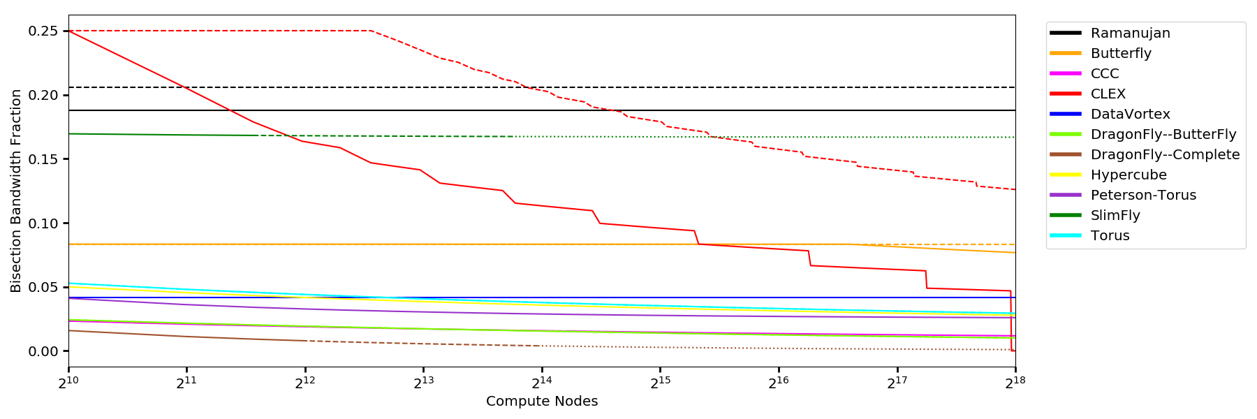
Figure 5: Proportional Bisection Bandwidth for supercomputing topologies by number of compute nodes.

We provide in Table LABEL:T:boundsBW a summary of the results on the bisection bandwidth and algebraic connectivity of the topologies considered in this work. Additionally, for comparison we provide bounds on the bisection bandwidth and algebraic connectivity for a similarly sized Ramanujan topology. We focus on bisection bandwidth in our comparison, although we remind the reader the spectral results summarized in Table LABEL:T:boundsBW also provide bounds on a plethora of other salient interconnection network properties (such as diameter, average distance, and fault tolerance) via the theorems mentioned in Section 2. As closer inspection of the table makes clear, for each of these topologies there is a significant gap between the achieved value and the minimum guaranteed to be achievable in an equivalent Ramanujan topology. However, assessing these results across families is more challenging due to different input parameters and parameter multiplicities for each topology. To better enable such a comparison, in Figure 5 we plot the proportional bisection bandwidth by number of compute nodes for each topology, as well as the minimum guaranteed by a Ramanujan topology. In general the solid lines represent those topologies with switches comparable to current topologies (that is, having radix at most 64 as in the Cray Slingshot Topology Cray:Slingshot ; Cray:XC while the dashed lines represent the proportional bisection bandwidth achievable with next generation switches (radix at most 128), and the dotted line represents those topologies that would require even higher radix switches. We note that even the limitations on the radix are not sufficient to uniquely determine the highest bisection bandwidth proportion for some topologies. Thus we will also impose following additional assumptions on the topologies with an aim of avoiding trivial instantiations of the topology:

• Butterfly: for the Butterfly topology we assume that there are at least 3 ranks of switches, i.e. $s\geq 3$,

• CLEX: for the CLEX topology we assume that there are at least two layers $\ell\geq 2$ and that the initial generating graph is the complete graph on at least 3 vertices,

• Data Vortex: for the Data Vortex we assume that there are at least 3 “cylinders”, i.e. $C\geq 3$,

• DragonFly – Butterfly: similarly to the Butterfly topology, for the DragonFly topology where the electrical network is given by a Butterfly network, we assume that $s\geq 3$, and

• Torus: for the torus topology we assume that all the cycles are non-degnerate, i.e. that $k\geq 3$.

Even as we compare these upper bounds on the best-possible bisection bandwidth for each topology against the worst-possible in a Ramanujan topology, we still observe a sizable gap, with the 128 radix SlimFly and CLEX topologies the closest to the Ramanujan lower bound. We suspect the region where CLEX outperforms Ramanujan graphs is an artifact of the looseness of the analysis of CLEX for small parameter settings, rather than a true reflection of the relative sizes of the bisection bandwidths.

In light of the beneficial structural properties of random graphs, it is natural to ask whether any potential utility of Ramanujan supercomputing topologies is already offered by randomized constructions, such as the well-known Jellyfish topology. Indeed, such topologies are touted for their low diameter, short average path lengths, and high bisection bandwidth singla2012jellyfish . Although random regular graphs are not quite Ramanujan, it is true that random $d$-regular graphs have good spectral expansion. Notably, Friedman’s celebrated proof Friedman2003 of Alon’s second eigenvalue conjecture Alon:EigenvaluesExpanders showed that if $G$ is a random $k$-regular graph on $n$ vertices then with probability going to 1 as $n\to\infty$, we have $\lambda(G)\leq 2\sqrt{k-1}+o(1)$. Thus, in the limiting sense, random regular graphs are “almost Ramanujan.” Nonetheless, randomized constructions are also limited as interconnection topologies in that they pose serious challenges for routing, physical layout, and wiring singla2012jellyfish . In these regards, structured topologies offer advantages.

Consequently, one may ask whether more structured families, such as Cayley graphs, might serve as a more amenable alternative to random constructions. Since many of the popular topologies can be phrased as Cayley graphs (e.g. the torus and hypercube topologies) or have a strong connections to Cayley graphs (e.g. the SlimFly and Peterson torus topologies) it is natural to speculate that a Cayley graph could serve as the basis of a strong supercomputing topology. Indeed, work Akers1987a investigating Cayley graphs as interconnection networks dates back to at least the 1980’s, see Heydemann1997 for a survey. In particular, abelian Cayley graphs may seem particularly promising because the classification of abelian groups gives a natural means of easily performing efficient routing. However, abelian Cayley graphs do not offer the spectral expansion of Ramanujan graphs: as a consequence of a result of Cioabă Cioaba:CayleySpectra there is a constant $C(k,\epsilon)$ such that if the group has more elements than $C(k,\epsilon)$, then any Cayley graph generated by a $k$-element set has algebraic connectivity at most $\epsilon$. Thus, for any fixed radix $k$, there does not exist an infinite family of radix $k$ abelian Cayley graphs which are Ramanujan.

Given these tradeoffs between randomized designs and highly structured Cayley graph designs, we believe the explicit Ramanujan construction by Lubotsky, Phillips, and Sarnak warrants further investigation as a candidate for supercomputing interconnection networks. By virtue of their optimal spectral expansion, LPS graphs offer many of the same (if not better) structural properties exhibited by random regular graphs. Yet, as highly structured Cayley graphs, LPS graphs may be more amenable to practical considerations and easier to develop efficient routing schemes for than random constructions. Indeed, recent work by Sardari Sardari2017 , as well as Pinto and Petit Pinto2018 investigating short paths in LPS graphs shows that, while sometimes challenging to analyze, the local structure of these topologies may be exploited for the purposes of routing. While the work we’ve done here attests to the structural benefits of LPS graphs over other supercomputing topologies, additional work is needed to better assess the benefits of utilizing LPS graphs as interconnection networks in practice.

- (1) Xpander project page. https://husant.github.io/Xpander/.
- (2) Bob Metcalfe eats his words, Internet Computing Online, 1 (1997).
- (3) Slingshot: The interconnect for the exascale era, tech. rep., Cray Inc., Febuary 2019.
- (4) A. Abiad, B. Brimkov, X. Martinez-Rivera, S. O, and J. Zhang, Spectral bounds for the connectivity of regular graphs with given order, Electronic Journal of Linear Algebra, 34 (2018), pp. 428–443.
- (5) Akers and Krishnamurthy, On group graphs and their fault tolerance, IEEE Transactions on Computers, C-36 (1987), pp. 885–888.
- (6) N. Alon, Eigenvalues and expanders, Combinatorica, 6 (1986), pp. 83–96. Theory of computing (Singer Island, Fla., 1984).
- (7) N. Alon, F. R. K. Chung, and R. L. Graham, Routing permutations on graphs via matchings, SIAM J. Discrete Math., 7 (1994), pp. 513–530.
- (8) N. Alon and V. Milman, , isoperimetric inequalities for graphs, and superconcentrators, Journal of Combinatorial Theory, Series B, 38 (1985), pp. 73–88.
- (9) N. Alon and J. H. Spencer, The probabilistic method, Wiley-Interscience Series in Discrete Mathematics and Optimization, Wiley-Interscience [John Wiley & Sons], New York, second ed., 2000. With an appendix on the life and work of Paul Erdős.
- (10) B. Alverson, E. Froese, L. Kaplay, and D. Roweth, Cray® XCTM Series Network.
- (11) M. Besta and T. Hoefler, Slim fly: A cost effective low-diameter network topology, in Proceedings of the International Conference for High Performance Computing, Networking, Storage and Analysis, IEEE Press, 2014, pp. 348–359.
- (12) A. Bhatele, N. Jain, Y. Livnat, V. Pascucci, and P. Bremer, Analyzing network health and congestion in dragonfly-based supercomputers, in 2016 IEEE International Parallel and Distributed Processing Symposium, IPDPS 2016, Chicago, IL, USA, May 23-27, 2016, 2016, pp. 93–102.
- (13) N. Biggs, Algebraic graph theory, Cambridge Mathematical Library, Cambridge University Press, Cambridge, second ed., 1993.
- (14) Y. Bilu and N. Linial, Lifts, discrepancy and nearly optimal spectral gap, Combinatorica, 26 (2006), pp. 495–519.
- (15) E. A. Brewer, F. T. Chong, and T. Leighton, Scalable expanders, in Proceedings of the twenty-sixth annual ACM symposium on Theory of computing - STOC ’94, ACM Press, 1994.
- (16) A. E. Brouwer and W. H. Haemers, Spectra of graphs, Universitext, Springer, New York, 2012.
- (17) R. A. Brualdi, The mutually beneficial relationship of graphs and matrices, vol. 115, American Mathematical Soc., 2011.
- (18) P. Buser, A note on the isoperimetric constant, Annales scientifiques de École normale supérieure, 15 (1982), pp. 213–230.
- (19) F. Chung, A generalized alon-boppana bound and weak ramanujan graphs, The Electronic Journal of Combinatorics, 23 (2016), pp. 3–4.
- (20) F. R. K. Chung, Diameters and eigenvalues, Journal of the American Mathematical Society, 2 (1989), pp. 187–187.
- (21) F. R. K. Chung, Spectral graph theory, vol. 92 of CBMS Regional Conference Series in Mathematics, Published for the Conference Board of the Mathematical Sciences, Washington, DC, 1997.
- (22) S. M. Cioabă, Closed walks and eigenvalues of abelian cayley graphs, Comptes Rendus Mathematique, 342 (2006), pp. 635 – 638.
- (23) M. B. Cohen, Ramanujan graphs in polynomial time, in 2016 IEEE 57th Annual Symposium on Foundations of Computer Science (FOCS), IEEE, oct 2016.
- (24) M. Fiedler, Algebraic connectivity of graphs, Czechoslovak mathematical journal, 23 (1973), pp. 298–305.
- (25) J. Friedman, A proof of alon’s second eigenvalue conjecture, in Proceedings of the thirty-fifth ACM symposium on Theory of computing - STOC ’03, ACM Press, 2003.
- (26) A. M. Frieze, Edge-disjoint paths in expander graphs, SIAM J. Comput., 30 (2001), pp. 1790–1801 (electronic).
- (27) R. Gioiosa, A. Tumeo, J. Yin, T. Warfel, D. Haglin, and S. Betelu, Exploring DataVortex systems for irregular applications, in 2017 IEEE International Parallel and Distributed Processing Symposium (IPDPS), IEEE, may 2017.
- (28) R. Gioiosa, T. Warfel, J. Yin, A. Tumeo, and D. Haglin, Exploring data vortex network architectures, in 2016 IEEE 24th Annual Symposium on High-Performance Interconnects (HOTI), IEEE, aug 2016.
- (29) C. Gkantsidis, M. Mihail, and A. Saberi, Conductance and congestion in power law graphs, SIGMETRICS Perform. Eval. Rev., 31 (2003), pp. 148–159.
- (30) C. Godsil and G. Royle, Algebraic graph theory, vol. 207 of Graduate Texts in Mathematics, Springer-Verlag, New York, 2001.
- (31) C. Hawkins, B. A. Small, D. S. Wills, and K. Bergman, The data vortex, an all optical path multicomputer interconnection network, IEEE Transactions on Parallel and Distributed Systems, 18 (2007), pp. 409–420.
- (32) M.-C. Heydemann, Cayley graphs and interconnection networks, in Graph Symmetry, Springer Netherlands, 1997, pp. 167–224.
- (33) S. Hoory, A lower bound on the spectral radius of the universal cover of a graph, J. Combin. Theory Ser. B, 93 (2005), pp. 33–43.
- (34) I. Iliadis, N. Chrysos, and C. Minkenberg, Performance evaluation of the data vortex photonic switch, IEEE Journal on Selected Areas in Communications, 25 (2007), pp. 20–35.
- (35) S. Jung-hyun, L. HyeongOk, and J. Moon-suk, Optimal routing and hamiltonian cycle in petersen-torus networks, Busan, South Korea, November 2008, IEEE.
- (36) S. Kar and J. M. Moura, Ramanujan topologies for decision making in sensor networks, in 44th Allerton Conference on Communication, Control, and Computing, Citeseer, 2006.
- (37) J. Kim, W. J. Dally, S. Scott, and D. Abts, Technology-driven, highly-scalable dragonfly topology, in 2008 International Symposium on Computer Architecture, IEEE, jun 2008.
- (38) J. Kleinberg and R. Rubinfeld, Short paths in expander graphs, in 37th Annual Symposium on Foundations of Computer Science (Burlington, VT, 1996), IEEE Comput. Soc. Press, Los Alamitos, CA, 1996, pp. 86–95.
- (39) G. F. Lawler and A. D. Sokal, Bounds on the spectrum for Markov chains and Markov processes: a generalization of Cheeger’s inequality, Trans. Amer. Math. Soc., 309 (1988), pp. 557–580.
- (40) F. T. Leighton, Introduction to parallel algorithms and architectures: Arrays· trees· hypercubes, Elsevier, 2014.
- (41) C. Lenzen and R. Wattenhofer, Clex: Yet another supercomputer architecture? arXiv 1607.00298v1, 2016.
- (42) A. Lubotzky, R. Phillips, and P. Sarnak, Ramanujan graphs, Combinatorica, 8 (1988), pp. 261–277.
- (43) A. Marcus, D. A. Spielman, and N. Srivastava, Interlacing families i: Bipartite ramanujan graphs of all degrees, in 2013 IEEE 54th Annual Symposium on Foundations of Computer Science, IEEE, oct 2013.
- (44) A. W. Marcus, D. A. Spielman, and N. Srivastava, Interlacing families IV: Bipartite ramanujan graphs of all sizes, in 2015 IEEE 56th Annual Symposium on Foundations of Computer Science, IEEE, oct 2015.
- (45) G. A. Margulis, Explicit group-theoretical constructions of combinatorial schemes and their application to the design of expanders and concentrators, Problemy peredachi informatsii, 24 (1988), pp. 51–60.
- (46) B. D. McKay, M. Miller, and J. Širáň, A note on large graphs of diameter two and given maximum degree, Journal of Combinatorial Theory, Series B, 74 (1998), pp. 110–118.
- (47) M. Miller and J. Sirán, Moore graphs and beyond: A survey of the degree/diameter problem, The electronic journal of combinatorics, 1000 (2005), pp. DS14–Dec.
- (48) B. Mohar, Eigenvalues, diameter, and mean distance in graphs, Graphs and combinatorics, 7 (1991), pp. 53–64.
- (49) B. Mohar, Y. Alavi, G. Chartrand, and O. Oellermann, The laplacian spectrum of graphs, Graph theory, combinatorics, and applications, 2 (1991), p. 12.
- (50) M. Morgenstern, Existence and explicit constructions of regular ramanujan graphs for every prime power , Journal of Combinatorial Theory, Series B, 62 (1994), pp. 44–62.
- (51) A. Nilli, On the second eigenvalue of a graph, Discrete Math., 91 (1991), pp. 207–210.
- (52) R. Paturi, D.-T. Lu, J. E. Ford, S. C. Esener, and S. H. Lee, Parallel algorithms based on expander graphs for optical computing, Applied Optics, 30 (1991), p. 917.
- (53) E. C. Pinto and C. Petit, Better path-finding algorithms in LPS ramanujan graphs, Journal of Mathematical Cryptology, 12 (2018), pp. 191–202.
- (54) F. P. Preparata and J. Vuillemin, The cube-connected cycles: a versatile network for parallel computation, Communications of the ACM, 24 (1981), pp. 300–309.
- (55) F. Prieto-Castrillo, A. Astillero, and M. Botón-Fernández, A stochastic process approach to model distributed computing on complex networks, Journal of Grid Computing, 13 (2014), pp. 215–232.
- (56) C. Riess, V. Strehl, and R. Wanka, The spectral relation between the cube-connected cycles and the shuffle-exchange network, PARS: Parallel-Algorithmen, -Rechnerstrukturen und -Systemsoftware, 29 (2012), pp. 15–26.
- (57) N. T. Sardari, Complexity of strong approximation on the sphere, arXiv:1703.02709.
- (58) A. Shacham, B. Small, O. Liboiron-Ladouceur, and K. Bergman, A fully implemented 12 12 data vortex optical packet switching interconnection network, Journal of Lightwave Technology, 23 (2005), pp. 3066–3075.
- (59) A. Sinclair and M. Jerrum, Approximate counting, uniform generation and rapidly mixing Markov chains, Inform. and Comput., 82 (1989), pp. 93–133.
- (60) A. Singla, C.-Y. Hong, L. Popa, and P. B. Godfrey, Jellyfish: Networking data centers randomly, in Presented as part of the 9th USENIX Symposium on Networked Systems Design and Implementation (NSDI 12), 2012, pp. 225–238.
- (61) R. M. Tanner, Explicit concentrators from generalized n-gons, SIAM Journal on Algebraic Discrete Methods, 5 (1984), pp. 287–293.
- (62) E. Upfal, An o(log n) deterministic packet-routing scheme, Journal of the ACM, 39 (1992), pp. 55–70.
- (63) A. Valadarsky, G. Shahaf, M. Dinitz, and M. Schapira, Xpander: Towards optimal-performance datacenters, in Proceedings of the 12th International on Conference on emerging Networking Experiments and Technologies - CoNEXT ’16, ACM Press, 2016.
- (64) V. V. Vazirani, Approximation algorithms, Springer-Verlag, Berlin, 2001.
- (65) D. B. West et al., Introduction to graph theory, vol. 2, Prentice hall Upper Saddle River, NJ, 1996.
- (66) Q. Yang and K. Bergman, Performances of the data vortex switch architecture under nonuniform and bursty traffic, Journal of Lightwave Technology, 20 (2002), pp. 1242–1247.
- (67) S. J. Young, The weighted spectrum of the universal cover and an Alon-Boppana result for the normalized Laplacian. preprint.