Axion scales and couplings with Stückelberg mixing

Abstract

We study the axion field range and low energy couplings in models with Stückelberg mixing between axions and $U(1)$ gauge bosons. It is noted that the gauge-invariant axion combination $\xi$ in the model is periodic modulo an appropriate shift of gauge-variant axions eaten by the massive $U(1)$ gauge bosons, which in some cases makes the connection between the field range and the low energy couplings less transparent. We derive the field range of $\xi$ for generic forms of the axion kinetic metric and $U(1)$ charges, and identify the field basis for which all non-derivative couplings of $\xi$ are quantized in a manner manifestly consistent with the periodicity of $\xi$. Generically Stückelberg mixing reduces the axion field range. In particular, the mixings between $N$ axions and $(N-1)$ $U(1)$ gauge bosons typically result in an exponentially reduced field range $M_{\xi}={\cal O}\left({k^{-(N-1)}f}/{\sqrt{N!}}\right)$ for the residual gauge-invariant axion $\xi$ in the limit $N\gg 1$ , where $f$ and $k$ denote the typical decay constant and the root mean square of the $U(1)$ gauge charges of the original $N$ axions. Using simple examples, we study also the reparameterization-invariant physical quantities such as the axion effective potential and 1PI couplings to gauge bosons, which are determined by the reparameterization-dependent axion couplings in the model.

1 Introduction

Axions (or axion-like particles) are considered to be one of the most compelling candidates for physics beyond the Standard Model of particle physics Kim:2008hd . Axions are periodic scalar fields and much of their low energy physics are determined by the mass scale $M_{a}$ called the axion decay constant which defines the field range of the canonically normalized axion as

$$a\equiv a+2\pi M_{a}.$$ (1)

There have been a variety of different axions introduced so far in particle physics and cosmology, and the favoured range of the decay constant of those axions differ by many orders of magnitudes. In most cases, $M_{a}$ is considered to be well below the Planck scale $M_{\rm Pl}$ Kim:2008hd , however in some cases it needs to be comparable to or even bigger than $M_{\rm Pl}$ Freese:1990rb ; Choi:1999xn ; Graham:2015cka . In theoretical side, it has been known for many years that potentially realistic string compactifications provide multiple axions whose decay constants are often of the order of ${g^{2}M_{\rm Pl}}/{8\pi^{2}}$, where $g$ is the gauge coupling in the model Witten:1984dg ; Choi:1985je ; Svrcek:2006yi ; Arvanitaki:2009fg . There has been also an argument called the weak gravity conjecture on axions ArkaniHamed:2006dz , implying that $M_{a}\lesssim{\cal O}({g^{2}M_{\rm Pl}}/{8\pi^{2}})$ within a theory defined at the scale of quantum gravity. Motivated by these, various mechanisms have been proposed to widen the possible range of $M_{a}$ in the low energy effective theory starting from a UV theory whose axion scales are limited to be within certain range ArkaniHamed:2003wu ; Kim:2004rp ; Bachlechner:2014gfa ; Dimopoulos:2005ac ; Junghans:2015hba ; Silverstein:2008sg ; Kaloper:2008fb ; Marchesano:2014mla ; Choi:2014rja ; Higaki:2014pja ; Bachlechner:2014hsa ; Ben-Dayan:2014zsa ; delaFuente:2014aca ; Shiu:2015uva ; Shiu:2015xda ; Brown:2015iha ; Hebecker:2015rya ; Choi:2015fiu ; Kaplan:2015fuy ; Giudice:2016yja ; Heidenreich:2015wga ; Shiu:2018unx ; Fonseca:2019aux ; Montero:2015ofa ; Bachlechner:2017zpb ; Bachlechner:2017hsj ; Rudelius:2014wla

In this paper, we wish to revisit one of such mechanisms, utilizing the Stückelberg mixing between axions and $U(1)$ gauge bosons Shiu:2015xda ; Shiu:2015uva ; Fonseca:2019aux . It has been noticed in Shiu:2015xda ; Shiu:2015uva that in some parameter limit of the Stückelberg mixing, the coupling $1/f_{\xi}$ of the canonically normalized gauge-invariant axion combination $\xi$ to non-Abelian gauge fields, i.e. $\frac{1}{32\pi^{2}}\frac{\xi}{f_{\xi}}G^{a\mu\nu}\tilde{G}^{a}_{\mu\nu}$, can be significantly smaller than the inverse of the mass scales introduced in the UV theory. Then, based on the expectation that $f_{\xi}$ is comparable to the axion decay constant $M_{\xi}$ which is defined by the axion periodicity $\xi\equiv\xi+2\pi M_{\xi}$, such suppression of $1/f_{\xi}$ was interpreted as an indication of the enhanced axion field range in the corresponding parameter limit. Recently the possibility of enhanced axion field range has been explored again with a simple model yielding an exponentially suppressed $1/f_{\xi}$ in a natural manner Fonseca:2019aux . On the other hand, in the presence of gauge-charged fermions, the axion coupling $1/f_{\xi}$ varies under the $\xi$-dependent phase rotation of fermion fields, while the axion field range $M_{\xi}$ is invariant under such field redefinition. In such case, the connection between the coupling $1/f_{\xi}$ and the axion decay constant $M_{\xi}$ depends on the choice of field basis, so deserves more careful analysis.

Recently the authors of Bonnefoy:2018ibr examined a model with clockwork-type Stückelberg mixings between $N$ axions and $(N-1)$ $U(1)$ gauge bosons, and noticed that $\xi$ is so well protected by the $(N-1)$ $U(1)$ gauge symmetries from getting a mass in the limit $N\gg 1$. As we will see, such protection of $\xi$ from being massive is deeply connected with the exponential reduction of the axion field range $M_{\xi}$ by the Stückelberg mixing in the limit $N\gg 1$. Therefore the previous studies suggest that Stückelberg mixing between axions and $U(1)$ gauge bosons can result in rich consequences in low energy axion physics. We wish to examine those consequences in a general framework which can cover all of the previous studies, while clarifying some confusions made in the previous works.

The organization of this paper is as follows. In the next section, we discuss the axion field range and low energy couplings in generic axion models with Stückelberg mixing. We first note that in such models the gauge-invariant axion combination $\xi$ is periodic modulo a shift of the gauge-variant axion combinations eaten by the massive $U(1)$ gauge bosons, which is determined by the kinetic metric and $U(1)$ gauge charges of the original axions. This often makes the connection between the field range and low energy couplings of $\xi$ less transparent. We then derive the field range of $\xi$ for generic forms of the axion kinetic metric and $U(1)$ charges, and discuss the axion couplings to matter and gauge fields, which depend on the choice of the matter field basis. We also identify the field basis for which all non-derivative couplings of $\xi$ are quantized in a manner manifestly consistent with the axion periodicity $\xi\equiv\xi+2\pi M_{\xi}$. It is noted also that Stückelberg mixing typically reduces the axion field range to a value smaller than the mass scales in the UV theory. In particular, for the case of Stückelberg mixing between $N$ axions and $(N-1)$ $U(1)$ gauge bosons, the axion field range is reduced as $M_{\xi}={\cal O}(k^{-(N-1)}f/\sqrt{N!})$ in the limit $N\gg 1$, where $f$ and $k$ denote the typical decay constant and the root mean square of the $U(1)$ gauge charges of the original $N$ axions.

In Sec. 3, we apply the results of Sec. 2 to specific examples to see the implications of our results. We first consider an illustrative simple model of Stückelberg mixing between two axions and a single $U(1)$ gauge boson. For this model, we study the reparameterization-invariant physical quantities such as the axion field range, axion 1PI amplitude to gauge bosons, and the axion effective potential induced by non-perturbative gauge dynamics, which are determined by the reparameterization-dependent axion couplings in the model. Another example is the model studied in Bonnefoy:2018ibr , involving $N$ axions which have a clockwork-type Stückelberg mixing with $(N-1)$ $U(1)$ gauge bosons. For this model, we examine the field range and low energy couplings of the gauge-invariant axion combination $\xi$, and discuss how much non-trivial it is to generate an effective potential of $\xi$ in the limit $N\gg 1$. Sec. 4 is the conclusion.

2 Axion field range and couplings with Stückelberg mixing

2.1 Stückelberg mixing between two axions and single $U(1)$ gauge boson

In this section, we examine the axion field range and low energy couplings in generic axion models with the Stückelberg mixing. For simplicity, we start with the case of two axions which have a Stückelberg mixing with single $U(1)_{A}$ gauge boson. In addition to $U(1)_{A}$, the model involves also a non-Abelian gauge symmetry which will be chosen to be $SU(N_{c})$ in the following discussion. At high scales above the Stückelberg mass, the lagrangian density is given by

$${\cal L} = \frac{1}{2}\sum_{ij}G_{ij}\left(\partial_{\mu}\theta^{i}-k^{i}A_{\mu}\right)\left(\partial^{\mu}\theta^{j}-k^{j}A^{\mu}\right)-\frac{1}{4g^{2}}F_{\mu\nu}F^{\mu\nu}-\frac{1}{4g_{a}^{2}}G^{a}_{\mu\nu}G^{a\mu\nu}$$ (2)

$$+\,\frac{1}{32\pi^{2}}\Big{(}\sum_{i}r_{i}\theta^{i}\Big{)}G^{a}_{\mu\nu}\tilde{G}^{a\mu\nu}+\frac{1}{32\pi^{2}}\Big{(}\sum_{i}s_{i}\theta^{i}\Big{)}F_{\mu\nu}\tilde{F}^{\mu\nu}$$

$$+\,\sum_{P}|D_{\mu}\phi_{P}|^{2}+\sum_{I}\bar{\psi}_{I}i\bar{\sigma}^{\mu}D_{\mu}\psi_{I}-\left(\mu_{IJ}e^{i\sum_{i}n^{IJ}_{i}\theta^{i}}\psi_{I}\psi_{J}+{\rm h.c.}\right)$$

$$-\,\left(\lambda_{IJP}e^{i\sum_{i}n^{IJP}_{i}\theta^{i}}\phi_{P}\psi_{I}\psi_{J}+{\rm h.c.}\right)+\sum_{i}(\partial_{\mu}\theta^{i}-k^{i}A_{\mu})J^{\mu}_{i}+\cdots,$$

where $\theta^{i}$ ($i=1,2$) are dimensionless axion fields normalized to have the $2\pi$ periodicity:

$$\theta^{i}\equiv\theta^{i}+2\pi,$$ (3)

$A_{\mu}$ and $G_{\mu}^{a}$ denote the $U(1)_{A}\times SU(N_{c})$ gauge fields, $\psi_{I}$ and $\phi_{P}$ are chiral fermions and complex scalar fields in the model, $J^{\mu}_{i}$ are gauge-invariant currents made of matter fields $\Phi=(\phi_{P},\psi_{I})$, and the ellipsis stands for possible additional terms including the gauge-invariant potential of $\theta^{i}$ and $\phi_{P}$. We assume that the (approximate) continuous shift symmetries $\theta^{i}\rightarrow\theta^{i}+{\rm constant}$ are good enough, so that the axion kinetic metric $G_{ij}$ is independent of $\theta^{i}$. Under $U(1)_{A}$, the fields transform as

$$U(1)_{A}:\ A_{\mu}\to A_{\mu}+\partial_{\mu}\Lambda,\quad\theta^{i}\to\theta^{i}+k^{i}\Lambda,\quad\Phi\to e^{-iq_{\Phi}\Lambda}\,\Phi\,\,\,\left(\Phi=\psi_{I},\phi_{P}\right),$$ (4)

where the $U(1)_{A}$ gauge transformation function $\Lambda(x)$ obeys the periodicity condition

$$\Lambda(x)\equiv\Lambda(x)+2\pi,$$ (5)

which ensures that the $U(1)_{A}$ charges $k^{i}$ and $q_{\Phi}$ have integer values. The axion $\theta^{i}$ can have a variety of non-derivative couplings to the gauge and matter fields, some of which are explicitly given and parametrized by $r_{i},s_{i},n^{IJ}_{i}$ and $n^{IJP}_{i}$ in (2), as well as the derivative couplings to the currents $J_{i}^{\mu}$. Here we choose the field basis for which the $2\pi$ periodicity of $\theta^{i}$ is manifest, i.e. the model is invariant under the discrete gauge symmetries

$$\mathbb{Z}_{i}:\,\,\,\theta^{i}\,\to\,\,\theta^{i}+2\pi\quad(i=1,2),$$ (6)

under which only $\theta^{i}$ transforms, while all other fields are invariant. In such field basis, the non-derivative coupling parameters $r_{i},s_{i},n^{IJ}_{i}$ and $n^{IJP}_{i}$ have integer values, which ensures that the model (2) is manifestly invariant under $\prod_{i}\mathbb{Z}_{i}$. Obviously the fermion mass parameter $\mu_{IJ}$ and the Yukawa coupling $\lambda_{IJP}$ can be nonzero only when the corresponding operators are invariant under $SU(N_{c})$, and also satisfy the following $U(1)_{A}$ invariance conditions:

$$q_{I}+q_{J}=\sum_{i}n^{IJ}_{i}k^{i},\quad q_{I}+q_{J}+q_{P}=\sum_{i}n^{IJP}_{i}k^{i}.$$ (7)

We consider the case that the fermions $\{\psi_{I}\}$ form a vector-like representation of $SU(N_{c})$, but can be chiral under $U(1)_{A}$. Then there can be nonzero $[U(1)_{A}]^{3}$ and $U(1)_{A}\times[SU(N_{c})]^{2}$ gauge anomalies, which should be cancelled by the $U(1)_{A}$ variation of the axion couplings $\theta^{i}F\tilde{F}$ and $\theta^{i}G\tilde{G}$. This requires

$$\sum_{I}q_{I}^{3}+\sum_{i}s_{i}k^{i}=2\sum_{I}q_{I}{\rm Tr}(T_{a}^{2}(\psi_{I}))+\sum_{i}r_{i}k^{i}=0,$$ (8)

where $T_{a}(\psi_{I})$ denotes the $SU(N_{c})$ generator for the fermion field $\psi_{I}$.

For our subsequent discussion, it is useful to define a complete set of integer-valued vectors and dual vectors in $\theta$-space, for which the integer-valued components of each vector are relatively prime. One such vector is provided by the $U(1)_{A}$ charges of $\theta^{i}$ as

$$\vec{k}_{r}=\left(k_{r}^{1},k_{r}^{2}\right)\equiv\frac{\left(k^{1},k^{2}\right)}{{\rm gcd}(\vec{k})},$$ (9)

where ${\rm gcd}(\vec{k})$ is the greatest common divisor of $k^{1}$ and $k^{2}$. We can construct the other linearly independent vector $\vec{\ell}=(\ell^{1},\ell^{2})$ and also the dual vectors $\vec{\tilde{k}}=(\tilde{k}_{1},\tilde{k}_{2})$ and $\vec{\tilde{\ell}}=(\tilde{\ell}_{1},\tilde{\ell}_{2})$ from the conditions:

$$\vec{\tilde{k}}\cdot\vec{k}_{r}=0,\quad\vec{\tilde{k}}\cdot\vec{\ell}=1,\quad\vec{\tilde{\ell}}\cdot\vec{\ell}=0,\quad\vec{\tilde{\ell}}\cdot\vec{k}_{r}=1.$$ (10)

For a given $\vec{k}$, the above conditions uniquely (up to sign) fix $\vec{\tilde{k}}$ as

$$\vec{\tilde{k}}=\pm(k_{r}^{2},-k_{r}^{1})=\pm\frac{(k^{2},-k^{1})}{{\rm gcd}(\vec{k})},$$ (11)

while $\vec{\ell}$ and $\vec{\tilde{\ell}}$ have additional degeneracy. For $\vec{\ell}$ and $\vec{\tilde{\ell}}$ satisfying (10), one easily finds

$$\vec{\ell}^{\prime}=\vec{\ell}+q\vec{k}_{r},\quad\vec{\tilde{\ell}}^{\prime}=\vec{\tilde{\ell}}-q\vec{\tilde{k}}$$ (12)

are also a solution, where $q$ is an arbitrary integer. At any rate, all solutions of (10) satisfy the identity

$$k_{r}^{i}\tilde{\ell}_{j}+\ell^{i}\tilde{k}_{j}=\delta^{i}_{j}$$ (13)

which turns out to be quite useful for our subsequent discussions. As we will see in the later part of this section, the above construction of the integer-valued vectors ($\vec{k}_{r},\vec{\ell}$) and dual vectors ($\vec{\tilde{k}},\vec{\tilde{\ell}})$ can be easily generalized to the more general case of $N(>2)$ axions which have the Stückelberg mixings with $(N-1)$ $U(1)$ gauge bosons.

In the above model, the $U(1)_{A}$ gauge boson gets a nonzero mass $gM_{A}$ through the Stückelberg mechanism, where

$$M_{A}^{2}(G,\vec{k})=\sum_{ij}G_{ij}k^{i}k^{j}.$$ (14)

It is then straightforward to rewrite the axion kinetic terms in terms of the gauge-invariant physical axion $\xi$ and the gauge-variant $\zeta$ eaten by the massive $U(1)_{A}$ gauge boson:

$$\frac{1}{2}\sum_{ij}G_{ij}(\partial_{\mu}\theta^{i}-k^{i}A_{\mu})(\partial^{\mu}\theta^{j}-k^{j}A^{\mu})=\frac{1}{2}(\partial_{\mu}\xi)^{2}+\frac{1}{2}M_{A}^{2}\left(A_{\mu}-{\partial_{\mu}\zeta}\right)^{2},$$ (15)

where

$$\xi=M_{\xi}\sum_{i}\tilde{k}_{i}\theta^{i},\quad\zeta=M_{A}^{-2}\sum_{ij}G_{ij}k^{i}\theta^{j}$$ (16)

for

$$M_{\xi}(G,\vec{k})=\frac{1}{\sqrt{\sum_{ij}(G^{-1})^{ij}\tilde{k}_{i}\tilde{k}_{j}}}.$$ (17)

Note that we use the convention that the gauge-variant $\zeta$ is dimensionless, while the gauge-invariant $\xi$ is a canonically normalized field with mass dimension one.

Using (16), the original field variable $\theta^{i}$ can be expressed in terms of $\zeta$ and $\xi$ as

$$\theta^{i}=k^{i}{\zeta}+\frac{\sum_{j}(G^{-1})^{ij}\tilde{k}_{j}}{\sum_{ij}(G^{-1})^{ij}\tilde{k}_{i}\tilde{k}_{j}}\,\frac{\xi}{M_{\xi}}.$$ (18)

To identify the periodicities of $\xi$ and $\zeta$, let us consider how $\xi$ and $\zeta$ transform under

$$\theta^{i}\to\theta^{i}+2\pi n^{i}$$ (19)

for generic integers $n^{i}$, which correspond to the discrete gauge transformations generated by (6). With the identity (13), one can make the decomposition

$$\frac{\sum_{j}(G^{-1})^{ij}\tilde{k}_{j}}{\sum_{i,j}(G^{-1})^{ij}\tilde{k}_{i}\tilde{k}_{j}}=\ell^{i}+\Gamma(G,\vec{k})k^{i},$$ (20)

where

$$\Gamma(G,\vec{k})=\frac{1}{{\rm gcd}(\vec{k})}\,\frac{\sum_{ij}(G^{-1})^{ij}\tilde{\ell}_{i}\tilde{k}_{j}}{\sum_{ij}(G^{-1})^{ij}\tilde{k}_{i}\tilde{k}_{j}},$$ (21)

and rewrite (18) as

$$\theta^{i}=k^{i}\zeta+\Big{(}\ell^{i}+\Gamma(G,\vec{k})k^{i}\Big{)}\frac{\xi}{M_{\xi}}.$$ (22)

Note that if one chooses different solutions of (10), e.g. $\vec{\ell}^{\prime}$ and $\vec{\tilde{\ell}}^{\prime}$ in (12), the corresponding $\Gamma$ is shifted as

$$\Gamma(G,\vec{k})\,\,\rightarrow\,\,\Gamma^{\prime}(G,\vec{k})=\Gamma(G,\vec{k})-\frac{q}{{\rm gcd}(\vec{k})}.$$ (23)

It is now straightforward to see that the discrete transformation (19) results in

$$\zeta \to \,\zeta+\frac{2\pi}{{\rm gcd}(\vec{k})}\sum_{i}\tilde{\ell}_{i}n^{i}-2\pi\Gamma(G,\vec{k})\sum_{i}\tilde{k}_{i}n^{i},$$

$$\xi \to \,\xi+2\pi M_{\xi}\sum_{i}\tilde{k}_{i}n^{i},$$ (24)

which are generated by

$$\mathbb{Z}_{\zeta}:\,\,\,\zeta\to\,\zeta+\frac{2\pi}{{\rm gcd}(\vec{k})},\quad\xi\to\,\xi,$$

$$\mathbb{Z}_{\xi}:\,\,\,\xi\to\,\xi+2\pi M_{\xi}(G,\vec{k}),\quad\zeta\to\,\zeta-2\pi\Gamma(G,\vec{k}).$$ (25)

In Fig.1, we depict $\mathbb{Z}_{\zeta}$ and $\mathbb{Z}_{\xi}$ in the axion moduli space of $\theta^{i}$. The discrete symmetry $\mathbb{Z}_{\zeta}$ involves only a shift of $\zeta$, so $\zeta$ is by itself a periodic field with the field range

$$\Delta\zeta=\frac{2\pi}{{\rm gcd}(\vec{k})}.$$ (26)

On the other hand, both $\xi$ and $\zeta$ are shifted under $\mathbb{Z}_{\xi}$, so $\xi$ is periodic with the field range

$$\Delta\xi=2\pi M_{\xi}(G,\vec{k})$$ (27)

only when the accompanying shift $\zeta\to\,\zeta-2\pi\Gamma(G,\vec{k})$ is taken into account. Note that $\Delta\zeta$ corresponds to the volume (length) of the $U(1)_{A}$ gauge orbit in the axion moduli space and the coordinate direction $\partial/\partial\xi$ is normal to the $U(1)_{A}$ gauge orbit w.r.t the metric $G_{ij}$ (See Fig. 1), so that

$$M_{A}\Delta\zeta\Delta\xi={\rm Vol}(\vec{\theta})=(2\pi)^{2}\sqrt{{\rm det}(G_{ij})},$$ (28)

where ${\rm Vol}(\vec{\theta})$ is the volume of the full axion moduli space.

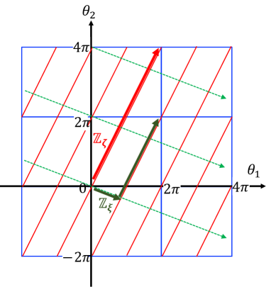
Figure 1: Illustration of the discrete gauge transformations $\mathbb{Z}_{\zeta}$ (thick red arrow) and $\mathbb{Z}_{\xi}$ (thick black arrow) in the moduli space of $\theta^{i}$. As an example, here we take $k_{1}=1$ and $k_{2}=2$. The red lines are the coordinate axis of $\zeta$, while the green lines are the coordinate axis of $\xi$. Note that $\partial\theta^{i}/\partial\zeta=k^{i}$ are integers, while $\partial\theta^{i}/\partial\xi$ are kinetic-metric-dependent continuous numbers, so the two coordinate axes are not orthogonal to each other.

In the original description using $\theta^{i}$, all non-derivative couplings of $\theta^{i}$ are quantized to be manifestly invariant under the $2\pi$ shifts of $\theta^{i}$. However, in the description using $\xi$ and $\zeta$, which is more convenient for describing low energy physics below the Stückelberg mass $M_{A}$, the connection between the periodicity and the non-derivative couplings of $\xi$ is less transparent as one needs to include the consequences of the accompanying shift $\zeta\to\,\zeta-2\pi\Gamma(G,\vec{k})$. This calls for a care when one attempts to deduce the field range $\Delta\xi$ from the couplings such as $\xi\,G^{a}_{\mu\nu}\tilde{G}^{a\mu\nu}$ Shiu:2015uva ; Fonseca:2019aux . In fact, the discrete symmetries $\mathbb{Z}_{\zeta}$ and $\mathbb{Z}_{\xi}$ have different realizations which are applicable even in the low energy limit where the massive $A_{\mu}-\partial_{\mu}\zeta$ is integrated out. Combining them with the $U(1)_{A}$ transformations (4) for $\Lambda=-2\pi/{\rm gcd}(\vec{k})$ (for $\mathbb{Z}_{\zeta}$) and $\Lambda=2\pi\Gamma(G,\vec{k})$ (for $\mathbb{Z}_{\xi}$), one finds the equivalent discrete symmetries under which only the light fields transform:

$$\mathbb{Z}_{\zeta}^{\prime}:\quad\xi\to\,\xi,\quad\Phi\to\,e^{i2\pi q_{\Phi}/{\rm gcd}(\vec{k})}\Phi,$$

$$\mathbb{Z}_{\xi}^{\prime}:\quad\xi\to\,\xi+2\pi M_{\xi},\quad\Phi\to\,e^{-i2\pi q_{\Phi}\Gamma}\Phi,$$ (29)

where $\Phi$ denotes the generic matter fields in the model. Obviously $\mathbb{Z}_{\zeta}^{\prime}$ corresponds to the discrete subgroup of $U(1)_{A}$ unbroken by the Stückelberg mechanism. As for $\mathbb{Z}_{\xi}^{\prime}$ which is associated with the periodicity of $\xi$, one can make the following $\xi$-dependent field redefinition:

$$\Phi\,\,\to\,\,\,\exp\left(-iq_{\Phi}\Gamma(G,\vec{k})\frac{\xi}{M_{\xi}}\right)\Phi,$$ (30)

after which the redefined $\Phi$ does not transform anymore. Then the discrete gauge symmetry for the periodicity of $\xi$ involves only a shift of $\xi$:

$$\mathbb{Z}_{\xi}^{\prime\prime}:\quad\xi\to\,\xi+2\pi M_{\xi}.$$ (31)

As it should be, the field redefinition (30) modifies the non-derivative couplings of $\xi$ in such a way that in the new field basis all non-derivative couplings are integer-multiples of $1/M_{\xi}$, so manifestly consistent with the axion periodicity $\xi\equiv\xi+2\pi M_{\xi}$. It modifies also the derivative couplings of $\xi$ by generating

$$\Delta{\cal L}_{\rm derivative}=\frac{\Gamma(G,\vec{k})}{M_{\xi}}\partial_{\mu}\xi(x)\sum_{\Phi}J^{\mu}_{\Phi},$$ (32)

where $J^{\mu}_{\Phi}$ is the $U(1)_{A}$ current of the matter field $\Phi$.

Let us see the connection between the axion periodicity and the axion couplings to matter and gauge fields more explicitly. We first consider the coupling to $SU(N_{c})$ gauge fields. Using (22), the couplings in the original field basis can be decomposed as

$$\frac{1}{32\pi^{2}}\Big{(}\sum_{i}r_{i}\theta^{i}\Big{)}G^{a}_{\mu\nu}\tilde{G}^{a\mu\nu}=\frac{1}{32\pi^{2}}\Big{(}\Big{(}\sum_{i}r_{i}k^{i}\Big{)}\zeta+\frac{\xi}{f_{\xi}}\Big{)}G^{a}_{\mu\nu}\tilde{G}^{a\mu\nu},$$ (33)

where

$$\frac{1}{f_{\xi}} = \frac{1}{M_{\xi}}\Big{(}\sum_{i}r_{i}\ell^{i}+\Gamma(G,\vec{k})\sum_{i}r_{i}k^{i}\Big{)}.$$ (34)

As we have anticipated, the coupling of $\zeta$ is manifestly consistent with the periodicity $\zeta\equiv\zeta+2\pi/{\rm gcd}(\vec{k})$. On the other hand, the coupling of $\xi$, i.e. $1/f_{\xi}$, contains a $G_{ij}$-dependent continuous piece in the unit of $1/M_{\xi}$, and therefore is not manifestly consistent with the periodicity $\xi\equiv\xi+2\pi M_{\xi}$. This is not surprising since we don’t include yet the effect of the discrete shift of $\zeta$ in $\mathbb{Z}_{\xi}$, or of the phase rotation of $\Phi$ in $\mathbb{Z}^{\prime}_{\xi}$, or of the field redefinition (30) for $\mathbb{Z}_{\xi}^{\prime\prime}$. As a specific choice, let us make the field redefinition (30). One of its consequences is the following change of lagrangian density through the anomalous variation of the path integral measure of $\psi_{I}$:

$$\Delta{\cal L}_{\rm anomaly} = \frac{1}{32\pi^{2}}\frac{\Gamma(G,\vec{k})}{M_{\xi}}\Big{(}2\sum_{I}q_{I}{\rm Tr}(T^{2}_{a}(\psi_{I}))\Big{)}\xi\,G^{a\mu\nu}\tilde{G}^{a}_{\mu\nu}$$ (35)

$$= -\frac{1}{32\pi^{2}}\frac{\Gamma(G,\vec{k})}{M_{\xi}}\Big{(}\sum_{i}r_{i}k^{i}\Big{)}\xi\,G^{a\mu\nu}\tilde{G}^{a}_{\mu\nu},$$

where we used the anomaly cancellation condition (8) for the latter expression. Including this change, the continuous piece of $1/f_{\xi}$ is cancelled and the coupling is modified to a quantized value which is manifestly consistent with the periodicity $\xi\equiv\xi+2\pi M_{\xi}$:

$$\frac{1}{f_{\xi}}\,\,\to\,\,\,\frac{1}{M_{\xi}}\sum_{i}r_{i}\ell^{i}.$$ (36)

The underlying $U(1)_{A}$ gauge symmetry assures that such modification applies for all non-derivative couplings of $\xi$. To see this, let us consider the coupling of $\xi$ to an operator ${\cal O}(\Phi)$ $({\cal O}(\Phi)=\psi_{I}\psi_{J},\,\phi_{P}\psi_{I}\psi_{J},...)$ whose $U(1)_{A}$ charge is $q_{\cal O}$, which would originate from

$$\exp\Big{(}i\sum_{i}n^{\cal O}_{i}\theta^{i}\Big{)}{\cal O}(\Phi),$$ (37)

where the $U(1)_{A}$ invariance requires that the integer-valued coefficients $n_{i}^{\cal O}$ satisfy

$$\sum_{i}n_{i}^{\cal O}k^{i}=q_{\cal O}.$$ (38)

As in the case of the coupling to $SU(N_{c})$ gauge fields, $\sum_{i}n_{i}^{\cal O}\theta^{i}$ can be expressed in terms of $\zeta$ and $\xi$ as

$$\sum_{i}n_{i}^{\cal O}\theta^{i}=\Big{(}\sum_{i}n_{i}^{\cal O}k^{i}\Big{)}\zeta+\Big{(}\sum_{i}n_{i}^{\cal O}\ell^{i}+\Gamma(G,\vec{k})\sum_{i}n_{i}^{\cal O}k^{i}\Big{)}\frac{\xi}{M_{\xi}}.$$ (39)

Again, under the field redefinition (30), ${\cal O}(\Phi)$ transforms as

$${\cal O}(\Phi)\,\,\rightarrow\,\,\exp\left(-iq_{\cal O}\Gamma(G,\vec{k})\frac{\xi}{M_{\xi}}\right){\cal O}(\Phi),$$ (40)

which results in the quantized non-derivative couplings of $\xi$ as

$$\exp\Big{(}i\sum_{i}n_{i}^{\cal O}\theta^{i}\Big{)}{\cal O}(\Phi)\,\,\rightarrow\,\,\exp\Big{(}i\sum_{i}n_{i}^{\cal O}\ell^{i}\frac{\xi}{M_{\xi}}\Big{)}{\cal O}(\Phi).$$ (41)

So, in the new field basis after the field redefinition (30), all non-derivative couplings of $\xi$ are given by inter-multiples of $1/M_{\xi}$, and therefore manifestly consistent with the axion periodicity $\xi\equiv\xi+2\pi M_{\xi}$, while the derivative couplings are shifted by the additional terms in (32).

Let us summarize the above discussions with a low energy effective theory obtained by integrating out the massive $U(1)_{A}$ gauge boson. The $U(1)_{A}$ gauge invariance admits to choose the unitary gauge $\zeta=0$ and integrate out $A_{\mu}$ using its equation of motion. For the model of (2), this results in the effective lagrangian density of the light axion $\xi$, gauge fields $G^{a}_{\mu}$ and matter fields $\Phi=(\phi_{P},\psi_{I})$, which is given by

$${\cal L}_{I} = \frac{1}{2}\partial_{\mu}\xi\partial^{\mu}\xi-\frac{1}{4g_{a}^{2}}G^{a}_{\mu\nu}G^{a\mu\nu}+\frac{1}{32\pi^{2}}\sum_{i}r_{i}(\ell^{i}+\Gamma(G,\vec{k})k^{i})\frac{\xi}{M_{\xi}}G^{a}_{\mu\nu}\tilde{G}^{a\mu\nu}$$ (42)

$$+\,\sum_{P}|D_{\mu}\phi_{P}|^{2}+\sum_{I}\bar{\psi}_{I}i\bar{\sigma}^{\mu}D_{\mu}\psi_{I}-\left(\mu_{IJ}e^{i\sum_{i}n^{IJ}_{i}(\ell^{i}+\Gamma(G,\vec{k})k^{i})\xi/M_{\xi}}\psi_{I}\psi_{J}+{\rm h.c.}\right)$$

$$-\,\left(\lambda_{IJP}e^{i\sum_{i}n^{IJP}_{i}(\ell^{i}+\Gamma(G,\vec{k})k^{i})\xi/M_{\xi}}\phi_{P}\psi_{I}\psi_{J}+{\rm h.c.}\right)$$

$$+\,\frac{\partial_{\mu}\xi}{M_{\xi}}\sum_{i}(\ell^{i}+\Gamma(G,\vec{k})k^{i})J^{\mu}_{i}+{\cal O}\left(\frac{1}{M_{A}^{2}}\right),$$

where ${\cal O}(1/M_{A}^{2})$ stands for the higher-dimensional effective interactions generated by the exchange of the massive $U(1)_{A}$ gauge field, and the ellipsis denotes the other possible terms including the potential of $\xi$ and $\phi_{P}$. Here we are using the same matter field basis as in the original model and the periodicity of $\xi$ is ensured by the discrete gauge symmetry (2.1):

$$\mathbb{Z}_{\xi}^{\prime}:\quad\xi\to\,\xi+2\pi M_{\xi},\quad\Phi\to\,e^{-i2\pi q_{\Phi}\Gamma}\Phi,$$ (43)

where $M_{\xi}$, $\Gamma(G,\vec{k})$ and $\vec{\ell},\vec{\tilde{k}},\vec{\tilde{\ell}}$ are defined in (17), (21) and (10), respectively. In the above, all non-derivative axion couplings are decomposed into two pieces, a piece quantized in the unit of $1/M_{\xi}$ and the other continuous piece proportional to $\Gamma(G,\vec{k})$. Obviously such decomposition is not unique, but has an ambiguity parametrized by integer as (12) and (23). The axion couplings in (42) assures that the continuous parts of all non-derivative couplings of $\xi$ can be rotated away by the field redefinition

$$\Phi\,\,\to\,\,\,e^{-iq_{\Phi}\Gamma\xi/M_{\xi}}\Phi,$$ (44)

after which the effective lagrangian density takes the form

$${\cal L}_{II} = \frac{1}{2}\partial_{\mu}\xi\partial^{\mu}\xi-\frac{1}{4g_{a}^{2}}G^{a}_{\mu\nu}G^{a\mu\nu}+\frac{1}{32\pi^{2}}\Big{(}\sum_{i}r_{i}\ell^{i}\Big{)}\frac{\xi}{M_{\xi}}G^{a}_{\mu\nu}\tilde{G}^{a\mu\nu}$$ (45)

$$+\,\sum_{P}D_{\mu}\phi_{P}^{*}D^{\mu}\phi_{P}+\sum_{I}\bar{\psi}_{I}i\bar{\sigma}^{\mu}D_{\mu}\psi_{I}-\left(\mu_{IJ}e^{i(\sum_{i}n^{IJ}_{i}\ell^{i})\xi/M_{\xi}}\psi_{I}\psi_{J}+{\rm h.c}\right)$$

$$-\,\left(\lambda_{IJP}e^{i(\sum_{i}n^{IJP}_{i}\ell^{i})\xi/M_{\xi}}\phi_{P}\psi_{I}\psi_{J}+{\rm h.c.}\right)$$

$$+\,\frac{\partial_{\mu}\xi}{M_{\xi}}\Big{(}\sum_{i}(\ell^{i}+\Gamma(G,\vec{k})k^{i})J^{\mu}_{i}+\Gamma(G,\vec{k})\sum_{\Phi}J^{\mu}_{\Phi}\Big{)}+{\cal O}\left(\frac{1}{M_{A}^{2}}\right),$$

so all non-derivative couplings of $\xi$ are quantized to be manifestly consistent with the axion periodicity $\xi\equiv\xi+2\pi M_{\xi}$.

In the above, we presented the low energy effective theory of the model (2) in two different field basis. It should be stressed that axion couplings to matter and/or gauge fields are basis-dependent, e.g. vary under axion-dependent phase rotation of matter fields, while their physical consequences should be basis-independent. In the next section, we will discuss this issue with a simple example.

2.2 Generalization to multiple ($N>2$) axions

It is in fact straightforward to generalize the discussion to more general cases, for instance models with $N(>2)$ axions having the Stückelberg mixings with $(N-1)$ $U(1)$ gauge bosons. In such models, the gauge invariant kinetic terms of axions can be written as

$${\cal L}_{\rm kin}=\frac{1}{2}\sum_{ij=1}^{N}G_{ij}\Big{(}\partial_{\mu}\theta^{i}-\sum_{\alpha=1}^{N-1}k^{i}_{\alpha}A^{\alpha}_{\mu}\Big{)}\Big{(}\partial^{\mu}\theta^{j}-\sum_{\beta=1}^{N-1}k^{j}_{\beta}A^{\beta\mu}\Big{)}$$ (46)

and the $U(1)$ gauge transformations of the fields are given by

$$U(1)_{\alpha}:\quad A^{\alpha}_{\mu}\to A^{\alpha}_{\mu}+\partial_{\mu}\Lambda^{\alpha},\quad\theta^{i}\to\theta^{i}+\sum_{\alpha}k^{i}_{\alpha}\Lambda^{\alpha},\quad\Phi\to e^{-i\sum_{\alpha}q_{\Phi\alpha}\Lambda^{\alpha}}\Phi,$$ (47)

where $\Phi$ denotes the gauge-charged matter fields in the model. Again $\theta^{i}$ and $\Lambda^{\alpha}$ are normalized to have the $2\pi$ periodicity, and then all $U(1)$ charges $k^{i}_{\alpha}$ and $q_{\Phi\alpha}$ have integer values. Constructing a complete set of the integer-valued vectors and dual vectors in the $\theta$-space is also useful here. For $N-1$ linearly independent vectors,

$$\vec{k}_{r\alpha}=(k_{r\alpha}^{1},\cdots,k^{N}_{r\alpha})\equiv\frac{(k^{1}_{\alpha},\cdots,k^{N}_{\alpha})}{{\rm gcd}(\vec{k}_{\alpha})}\quad{\rm for}\quad\alpha=1,2,\cdots,N-1,$$ (48)

we can find the remaining vector $\vec{\ell}$ and the $N$ dual vectors $\vec{\tilde{k}},\vec{\tilde{\ell}}^{\alpha}$ from

$$\vec{\tilde{k}}\cdot\vec{k}_{r\alpha}=0,\quad\vec{\tilde{k}}\cdot\vec{\ell}=1,\quad\vec{\tilde{\ell}}^{\alpha}\cdot\vec{k}_{r\beta}=\delta^{\alpha}_{\beta},\quad\vec{\tilde{\ell}}^{\alpha}\cdot\vec{\ell}=0\quad{\rm for}\quad\alpha,\beta=1,2,\cdots,N-1.$$ (49)

As in the case of two axion model, $\vec{\tilde{k}}$ is determined uniquely (up to sign) by the $U(1)_{A}$ charge vectors $\vec{k}_{r\alpha}$ as

$$\tilde{k}_{i}=\pm\det\left[\begin{array}[]{cccc}\delta^{1}_{i}&\delta^{2}_{i}&\cdots&\delta^{N}_{i}\\ k^{1}_{r1}&k^{2}_{r1}&\cdots&k^{N}_{r1}\\ k^{1}_{r2}&k^{2}_{r2}&\cdots&k^{N}_{r2}\\ \vdots&\vdots&\ddots&\vdots\\ k^{1}_{rN-1}&k^{2}_{rN-1}&\cdots&k^{N}_{rN-1}\end{array}\right].$$ (55)

For given $\vec{k}_{r\alpha}$ and $\vec{\tilde{k}}$, the corresponding $\vec{\ell}$ and $\vec{\tilde{\ell}}^{\alpha}$ are not unique as the conditions in (49) are invariant under the reparameterization

$$\vec{\ell}\,\,\to\,\,\vec{\ell}^{\prime}=\vec{\ell}+\sum_{\alpha}q^{\alpha}\vec{k}_{r\alpha},\quad\vec{\tilde{\ell}}^{\alpha}\,\,\to\,\,\vec{\tilde{\ell}}^{\alpha\prime}=\vec{\tilde{\ell}}^{\alpha}-q^{\alpha}\vec{\tilde{k}},$$ (56)

where $q^{\alpha}$ ($\alpha=1,2,\cdots,N-1$) are arbitrary independent integers. However such degeneracy of $\vec{\ell}$ and $\vec{\tilde{\ell}}^{\alpha}$ does not matter to us as all solutions satisfy the common completeness relation

$$\sum_{\alpha}k^{i}_{r\alpha}\tilde{\ell}^{\alpha}_{j}+\ell^{i}\tilde{k}_{j}=\delta^{i}_{j}.$$ (57)

Again, one can express the original axion fields $\theta^{i}$ in terms of the canonically normalized gauge-invariant $\xi$ and the gauge-variant $\zeta^{\alpha}$ eaten by $A_{\mu}^{\alpha}$:

$$\theta^{i}=\sum_{\alpha=1}^{N-1}k^{i}_{\alpha}\zeta^{\alpha}+\frac{\sum_{j=1}^{N}(G^{-1})^{ij}\tilde{k}_{j}}{\sum_{ij}(G^{-1})^{ij}\tilde{k}_{i}\tilde{k}_{j}}\frac{\xi}{M_{\xi}}$$ (58)

for which the axion kinetic terms (46) take the familiar form

$${\cal L}_{\rm kin}=\frac{1}{2}(\partial^{\mu}\xi)^{2}+\frac{1}{2}\sum_{\alpha\beta}(M_{A}^{2})_{\alpha\beta}(A_{\mu}^{\alpha}-\partial_{\mu}\zeta^{\alpha})(A^{\mu\beta}-\partial^{\mu}\zeta^{\beta}),$$ (59)

where

$$(M_{A}^{2})_{\alpha\beta}=\sum_{ij}G_{ij}k^{i}_{\alpha}k^{j}_{\beta},\quad M^{2}_{\xi}=\frac{1}{\sum_{ij}(G^{-1})^{ij}\tilde{k}_{i}\tilde{k}_{j}}.$$ (60)

Obviously $(M_{A}^{2})_{\alpha\beta}$ is the mass matrix of the $(N-1)$ massive $U(1)$ gauge bosons. As in the case of two axion model, we will see that $M_{\xi}$ corresponds to the decay constant of $\xi$, i.e. the field range of $\xi$ is given by $\Delta\xi=2\pi M_{\xi}$. From (58), we find also

$$\frac{\xi}{M_{\xi}}=\sum_{i}\tilde{k}_{i}\theta^{i},\quad\zeta^{\alpha}=\sum_{ij\beta}\left(M^{-2}_{A}\right)^{\alpha\beta}G_{ij}k^{i}_{\beta}\theta^{j},$$ (61)

Using the identity (57), one can rewrite (58) as

$$\theta^{i}=\sum_{\alpha=1}^{N-1}k^{i}_{\alpha}\zeta^{\alpha}+\Big{(}\ell^{i}+\sum_{\alpha=1}^{N-1}\Gamma^{\alpha}(G,\vec{k}_{\alpha})k^{i}_{\alpha}\Big{)}\frac{\xi}{M_{\xi}},$$ (62)

where

$$\Gamma^{\alpha}(G,\vec{k}_{\alpha})=\frac{1}{{\rm gcd}(\vec{k}_{\alpha})}\frac{\sum_{ij}(G^{-1})^{ij}\tilde{\ell}_{i}^{\alpha}\tilde{k}_{j}}{\sum_{ij}(G^{-1})^{ij}\tilde{k}_{i}\tilde{k}_{j}}.$$ (63)

With the above expression, one can see that the discrete gauge symmetries for the $2\pi$ periodicities of $\theta^{i}$, i.e.

$$\mathbb{Z}_{i}:\,\,\,\theta^{i}\,\,\to\,\theta^{i}+2\pi\quad(i=1,\cdots,N),$$ (64)

are generated by

$$\mathbb{Z}_{\zeta^{\alpha}}: \zeta^{\alpha}\,\,\to\,\zeta^{\alpha}+\frac{2\pi}{{\rm gcd}(\vec{k}_{\alpha})}\quad(\alpha=1,\cdots,N-1),$$

$$\mathbb{Z}_{\xi}: \xi\,\,\to\,\xi+2\pi M_{\xi},\quad\zeta^{\alpha}\,\,\to\,\zeta^{\alpha}-2\pi\Gamma^{\alpha}(G,\vec{k}_{\alpha}).$$ (65)

One can consider also the equivalent discrete symmetries which do not involve a transformation of the massive $\zeta^{\alpha}$:

$$\mathbb{Z}_{\zeta^{\alpha}}^{\prime} = \mathbb{Z}_{\zeta^{\alpha}}\times\left.U(1)_{\alpha}\right|_{\Lambda^{\alpha}=\frac{-2\pi}{{\rm gcd}(\vec{k}_{\alpha})}}:\quad\xi\to\xi,\quad\Phi\to e^{i2\pi q_{\Phi_{\alpha}}/{\rm gcd}(\vec{k}_{\alpha})}\Phi,$$

$$\mathbb{Z}_{\xi}^{\prime} = \mathbb{Z}_{\xi}\times\prod_{\alpha}\left.U(1)_{\alpha}\right|_{\Lambda^{\alpha}=2\pi\Gamma^{\alpha}}:\quad\xi\to\,\xi+2\pi M_{\xi},\quad\Phi\to\,e^{-i2\pi\sum_{\alpha}q_{\Phi_{\alpha}}\Gamma^{\alpha}}\Phi.$$ (66)

As for $\mathbb{Z}_{\xi}^{\prime}$ which is associated with the periodicity of $\xi$, one can make the $\xi$-dependent field redefinition

$$\Phi\,\,\to\,\,\,\exp\left(-i\sum_{\alpha}q_{\Phi_{\alpha}}\Gamma^{\alpha}(G,\vec{k}_{\alpha})\frac{\xi}{M_{\xi}}\right)\Phi,$$ (67)

after which the periodicity of $\xi$ is assured by

$$\mathbb{Z}_{\xi}^{\prime\prime}:\quad\xi\to\,\xi+2\pi M_{\xi},\quad\Phi\to\,\Phi.$$ (68)

As in the case of two axion model, the above field redefinition provides a field basis for which all non-derivative couplings of $\xi$ are quantized in the unit of $1/M_{\xi}$ in a manner manifestly consistent with the axion periodicity $\xi\equiv\xi+2\pi M_{\xi}$.

Models of $N(>2)$ axions which have the Stückelberg mixings with $(N-1)$ $U(1)$ gauge bosons exhibit several distinctive features in the limit $N\gg 1$. First of all, in such limit $\xi$ has a field range exponentially suppressed relative to the original axion scales encoded in the axion kinetic metric $G_{ij}$. To see this, let us note that $M_{\xi}$ is bounded as

$$\frac{f_{\rm min}}{||\tilde{k}||}\leq M_{\xi}\leq\frac{f_{\rm max}}{||\tilde{k}||},$$ (69)

where $f^{2}_{\rm max}$ and $f^{2}_{\rm min}$ denote the maximum and minimum eigenvalues of $G_{ij}$, and

$$||\tilde{k}||\equiv\Big{(}\sum_{i}\tilde{k}_{i}\tilde{k}_{i}\Big{)}^{1/2}.$$ (70)

It was shown in Choi:2014rja that $||\tilde{k}||$ determined by (55) grows exponentially in the limit $N\gg 1$:

$$||\tilde{k}||\sim(k^{i}_{r\alpha})_{\rm rms}^{N-1}\sqrt{N!},$$ (71)

where $(k^{i}_{r\alpha})_{\rm rms}$ is the root-mean-square of the normalized $U(1)$ charges:

$$(k^{i}_{r\alpha})_{\rm rms}=\sqrt{\frac{\sum_{i\alpha}(k^{i}_{r\alpha})^{2}}{N(N-1)}}\quad\Big{(}k^{i}_{r\alpha}=\frac{k^{i}_{\alpha}}{{\rm gcd}(\vec{k}_{\alpha})}\Big{)}.$$ (72)

In the clockwork axion models Choi:2014rja ; Choi:2015fiu ; Kaplan:2015fuy ; Giudice:2016yja , a large value of $||\tilde{k}||$ results in an enlarged field range of the light axion combination as $||\tilde{k}||$ can be interpreted as the number of windings along the light axion direction. On the other hand, in the Stückelberg axion models under discussion, a large $||\tilde{k}||$ means an enlarged volume of the gauge orbit of $\prod U(1)_{\alpha}$ in the axion moduli space of $\theta^{i}$. As a consequence, it results in a reduction of the field range of the gauge-invariant axion combination which is normal to the gauge orbit of $\prod U(1)_{\alpha}$. Specifically, for

$$G_{ij}\sim f^{2}\delta_{ij},$$ (73)

the axion field range is reduced as

$$M_{\xi}\sim\frac{1}{(k^{i}_{r\alpha})_{\rm rms}^{N-1}\sqrt{N!}}\,f,$$ (74)

which is exponentially smaller than the original axion scale $f$.

Stückelberg axion models in the limit $N\gg 1$ have an unusual feature which may cause a confusion in some case. In the original field basis without making any $\xi$-dependent field redefinition, all (both derivative and non-derivative) couplings of $\xi$ are determined simply by the couplings of $\theta^{i}$ and the wavefunction mixing between $\theta^{i}$ and $\xi$, which is given by (see(58))

$$\langle\theta^{i}|\xi\rangle=\frac{\sum_{j=1}^{N}(G^{-1})^{ij}\tilde{k}_{j}}{\sum_{ij}(G^{-1})^{ij}\tilde{k}_{i}\tilde{k}_{j}}\frac{1}{M_{\xi}}.$$ (75)

As $\theta^{i}$ are angular fields with $2\pi$ periodicity, their couplings can be described by dimensionless parameters, e.g. the integer coefficients $r_{i},s_{i},n_{i}^{IJ},n_{i}^{IJP}$ for the non-derivative couplings in (2) and also the continuous parameters $\kappa_{\psi_{I}}^{i},\kappa_{\phi_{P}}^{i}$ describing the derivative couplings of the form:

$$D_{\mu}\theta^{i}J^{\mu}_{i}=D_{\mu}\theta^{i}\left(\kappa_{\psi_{I}}^{i}\bar{\psi}_{I}\sigma^{\mu}\psi_{I}+i\kappa_{\phi_{P}}^{i}(\phi_{P}^{*}D_{\mu}\phi_{P}-\phi_{P}D_{\mu}\phi^{*}_{P})+...\right).$$ (76)

If the model does not involve any large dimensionless coupling or large number of fields, which might be required for a sensible UV behavior of the model, those couplings of $\theta^{i}$ are all expected to be of order unity or smaller. On the other hand, for $G_{ij}\sim f^{2}\delta_{ij}$, the wavefunction mixing (75) is bounded as

$$\langle\theta^{i}|\xi\rangle\lesssim\frac{1}{||\tilde{k}||}\frac{1}{M_{\xi}}\sim\frac{1}{f}.$$ (77)

This implies that in the original field basis all (both derivative and non-derivative) couplings of $\xi$ are of the order of $1/f$ or smaller if the couplings of $\theta^{i}$ are of order unity or smaller, which is exponentially weaker than the strength $\sim 1/M_{\xi}$ in the limit $N\gg 1$. On the other hand, we already noticed that after the $\xi$-dependent field redefinition (67), all non-derivative couplings of $\xi$ are quantized in the unit of $1/M_{\xi}$, so either exactly zero or of the order of $1/M_{\xi}$. If any of those quantized non-derivative couplings is nonzero, some derivative couplings should be of the order of $1/M_{\xi}$ in the new field basis due to the pieces induced by the field redefinition (67). This means that in the limit $N\gg 1$ axion couplings to matter and gauge fields have hierarchically different size in the two field bases related by the field redefinition (67). Since all physical consequences of the model should be independent of the choice of field basis, if one uses the new field basis, then there should be a fine cancellation between the contributions from different couplings of ${\cal O}(1/M_{\xi})$ to make the total result to be of the order of $1/f\ll 1/M_{\xi}$ as suggested by the couplings in the original field basis.

As a related feature, in Stückelberg axion models in the limit $N\gg 1$, $\xi$ is so well protected by the $(N-1)$ $U(1)$ gauge symmetries from getting a mass, and therefore can be ultra-light in a natural way. This was noticed before in Bonnefoy:2018ibr for a specific model with clockwork-type $U(1)$ gauge charges of $\theta^{i}$. In fact, this is a consequence of the exponentially large $||\tilde{k}||$, so a generic feature of the Stückelberg axion models in the limit $N\gg 1$. To see this, let us consider the constraint on the axion potential from the $U(1)$ gauge symmetries. In the prescription where the $2\pi$ periodicities of all $\theta^{i}$ are manifest, any non-trivial axion potential should be a periodic function of the gauge-invariant combination of $\theta^{i}$, i.e.

$$V_{\rm eff}=V_{\rm eff}\Big{(}\sum_{i}L_{i}\theta^{i}\Big{)}$$ (78)

for integer coefficients $L_{i}=L\tilde{k}_{i}$ where $L$ is a non-zero integer, for which

$$\sum_{i}L_{i}\theta^{i}=L\frac{\xi}{M_{\xi}}.$$ (79)

As $||\tilde{k}||$ is exponentially large in the limit $N\gg 1$, some $L_{i}$ should be exponentially large also. This means that any mechanism to generate an axion potential should provide those large integer coefficient $L_{i}$. The required large $L_{i}$ might be achieved by introducing many degrees of freedom or operators with very high mass dimensions as discussed in Bonnefoy:2018ibr . In any case, generically the requirement of exponentially large $L_{i}$ provides a strong constraint on the mechanism to generate an axion potential, and usually makes the induced axion potential highly suppressed. In the next section, we will present an explicit model of $N(>2)$ axions $\theta^{i}$ whose gauge charges for $(N-1)$ $U(1)$ symmetries have a clockwork pattern Bonnefoy:2018ibr , and study the behavior of the model in the limit $N\gg 1$.

3 Implications with examples

In the previous section, we derived the field range of the gauge-invariant axion combination $\xi$ and examined the structure of its couplings in generic models with the Stückelberg mixing between axions and $U(1)$ gauge bosons. In this section, we apply our results to the two specific examples to see some implications of our results explicitly.

3.1 An illustrative simple model

Our first example is a simple model involving two axions $\vec{\theta}=(\theta^{1},\theta^{2})$ and single $U(1)_{A}$ gauge boson, which was discussed recently in Fonseca:2019aux . The model has a simple form of kinetic metric:

$$G=\left(\begin{array}[]{cc}\ f_{1}^{2}&\ 0\\ 0&\ f_{2}^{2}\end{array}\right)$$ (82)

and the $U(1)_{A}$ gauge charge of $\vec{\theta}$:

$$\vec{k}=(1,1).$$ (83)

For this model, we will examine the reparameterization-invariant physical quantities such as the axion field range, the axion 1PI amplitude to gauge bosons, and the axion effective potential induced by non-perturbative gauge dynamics, which can be determined by the reparameterization-dependent axion couplings in the model.

For the above $U(1)_{A}$ charge vector $\vec{k}$, the corresponding $\vec{\tilde{k}}$, $\vec{\ell}$ and $\vec{\tilde{\ell}}$ satisfying (10) can be easily found to be

$$\vec{\tilde{k}}=(1,-1),\quad\vec{\ell}=(1,0),\quad\vec{\tilde{\ell}}=(0,1).$$ (84)

We may take different $\vec{\ell}$ and $\vec{\tilde{\ell}}$ given by (12), but all physical consequences should be the same. According to our results in the previous section, the gauge-invariant axion combination $\xi$ and the gauge-variant $\zeta$ eaten by the $U(1)_{A}$ gauge boson are given by

$$\xi = M_{\xi}\sum_{i}\tilde{k}_{i}\theta^{i}=M_{\xi}(\theta^{1}-\theta^{2}),$$

$$\zeta = M_{A}^{-2}\sum_{ij}G_{ij}k^{i}\theta^{j}=\frac{f_{1}^{2}\theta^{1}+f_{2}^{2}\theta^{2}}{f_{1}^{2}+f_{2}^{2}},$$ (85)

where

$$M_{A}^{2} = \sum_{ij}G_{ij}k^{i}k^{j}=f_{1}^{2}+f_{2}^{2},$$

$$M_{\xi}^{2} = \frac{1}{\sum_{ij}(G^{-1})^{ij}\tilde{k}_{i}\tilde{k}_{j}}=\frac{f_{1}^{2}f_{2}^{2}}{f_{1}^{2}+f_{2}^{2}},$$ (86)

and the $U(1)_{A}$ gauge boson mass and the field range of $\xi$ are determined as $gM_{A}$ and $\Delta\xi=2\pi M_{\xi}$, respectively. Equivalently, the original angular axions $\vec{\theta}$ can be decomposed as

$$\vec{\theta}=\vec{k}\,\zeta+\Big{(}\vec{\ell}+\Gamma(G,\vec{k})\,\vec{k}\Big{)}\frac{\xi}{M_{\xi}},$$ (87)

where

$$\Gamma(G,\vec{k})=\frac{\sum_{ij}(G^{-1})^{ij}\tilde{\ell}_{i}\tilde{k}_{j}}{\sum_{ij}(G^{-1})^{ij}\tilde{k}_{i}\tilde{k}_{j}}=-\frac{f_{1}^{2}}{f_{1}^{2}+f_{2}^{2}}.$$ (88)

Let us consider the possible axion couplings to gauge and matter fields in this model. In Fonseca:2019aux , it was noticed that this model can give a highly suppressed coupling of $\xi$ to non-Abelian gauge bosons in the parameter limit

$$f_{1}\gg f_{2}.$$ (89)

This observation is based on the coupling

$$\frac{1}{32\pi^{2}}\vec{r}\cdot\vec{\theta}\,G^{a}_{\mu\nu}\tilde{G}^{a\mu\nu}\quad\mbox{with}\quad\vec{r}=(1,0),$$ (90)

which results in

$$\frac{1}{32\pi^{2}}\frac{\xi}{f_{\xi}}G^{a}_{\mu\nu}\tilde{G}^{a\mu\nu},\$$ (91)

where

$$\frac{1}{f_{\xi}}=\frac{1}{M_{\xi}}\Big{(}\vec{r}\cdot\vec{\ell}+\Gamma(G,\vec{k})\,\vec{r}\cdot\vec{k}\Big{)}=\frac{f_{2}^{2}}{f_{1}^{2}+f_{2}^{2}}\frac{1}{M_{\xi}}.$$ (92)

Then in the limit $f_{1}\gg f_{2}$, the effective coupling $1/f_{\xi}$ is much smaller than the size ($\sim 1/M_{\xi}$) one would naively expect from the axion field range $\Delta\xi=2\pi M_{\xi}$. On the other hand, the above expression of $1/f_{\xi}$ shows that the big suppression of $1/f_{\xi}$ relative to $1/M_{\xi}$ is possible only when the coupling (90) is not gauge-invariant by itself, i.e. only when $\vec{r}\cdot\vec{k}\neq 0$. Note that if $\vec{r}\cdot\vec{k}=0$, then $1/f_{\xi}=(\vec{r}\cdot\vec{\ell})/M_{\xi}$ is an integer multiple of $1/M_{\xi}$ as expected. If $\vec{r}\cdot\vec{k}\neq 0$, the model should include gauge-charged chiral fermions whose mixed $U(1)_{A}\times[SU(N_{c})]^{2}$ anomaly cancels the $U(1)_{A}$ variation of the coupling (90). In the presence of such chiral fermions, the coupling $1/f_{\xi}$ varies under the $\xi$-dependent phase rotation of fermion fields, implying that the suppression of $1/f_{\xi}$ is an artifact of the particular choice of field basis, so needs more careful interpretation.

To see this, let us introduce the required fermions which can cancel the $U(1)_{A}$ variation of (90):

$$\psi=(N_{c},q_{\psi}),\quad\chi=(\bar{N}_{c},q_{\chi}),$$ (93)

where $N_{c}$ and $\bar{N}_{c}$ denote the fundamental and anti-fundamental representation of $SU(N_{c})$, and $q_{\psi,\chi}$ are the $U(1)_{A}$ charges of $\psi,\chi$. Then the generic axion couplings to gauge and matter fields take the form

$${\cal L}_{\rm int} = \frac{1}{32\pi^{2}}\vec{r}\cdot\vec{\theta}\,G^{a}_{\mu\nu}\tilde{G}^{a\mu\nu}-\left(\mu e^{i\vec{n}\cdot\vec{\theta}}\psi\chi+{\rm h.c.}\right)+\sum_{\psi_{I}=\psi,\chi}\vec{\kappa}_{\psi_{I}}\cdot D_{\mu}\vec{\theta}\,\bar{\psi}_{I}\sigma^{\mu}\psi_{I}$$ (94)

$$= \frac{c_{g}}{32\pi^{2}}\frac{\xi}{M_{\xi}}G^{a}_{\mu\nu}\tilde{G}^{a\mu\nu}-\left(\mu e^{ic_{\mu}\xi/M_{\xi}}\psi\chi+{\rm h.c}\right)+\frac{\partial_{\mu}\xi}{M_{\xi}}\sum_{\psi_{I}=\psi,\chi}c_{\psi_{I}}\bar{\psi}_{I}\sigma^{\mu}\psi_{I},$$

where the gauge-variant $\zeta$ is integrated out in the latter expression. The $U(1)_{A}$ invariance of the model requires

$$q_{\psi}+q_{\chi}=\vec{r}\cdot\vec{k}=1,\qquad\vec{n}\cdot\vec{k}=n_{1}+n_{2}=q_{\psi}+q_{\chi}=1,$$ (95)

where the first condition is for the cancellation of the $U(1)_{A}\times[SU(N_{c})]^{2}$ anomaly. Then the four axion couplings $c_{g},c_{\mu}$ and $c_{\psi_{I}}$ ($\psi_{I}=\psi,\chi$) are given by

$$c_{g} = \vec{r}\cdot\vec{\ell}+\Gamma(G,\vec{k})\,\vec{r}\cdot\vec{k}=\frac{f_{2}^{2}}{f_{1}^{2}+f_{2}^{2}},$$

$$c_{\mu} = \vec{n}\cdot\vec{\ell}+\Gamma(G,\vec{k})\,\vec{n}\cdot\vec{k}=\frac{n_{1}f_{2}^{2}-(1-n_{1})f_{1}^{2}}{f_{1}^{2}+f_{2}^{2}},$$

$$c_{\psi_{I}} = \vec{\kappa}_{\psi_{I}}\cdot\vec{\ell}+\Gamma(G,\vec{k})\,\vec{\kappa}_{\psi_{I}}\cdot\vec{k}=\frac{\kappa_{\psi_{I}1}f_{2}^{2}-\kappa_{\psi_{I}2}f_{1}^{2}}{f_{1}^{2}+f_{2}^{2}}.$$ (96)

We can now consider the two parameter family of $\xi$-dependent field redefinition:

$$\psi\,\to\,e^{ix_{\psi}\xi/M_{\xi}}\psi,\quad\chi\,\to\,e^{ix_{\chi}\xi/M_{\xi}}\chi,$$ (97)

under which the axion couplings vary as

$$c_{g}\,\to\,c_{g}+x_{\psi}+x_{\chi},\quad c_{\mu}\,\to\,c_{\mu}+x_{\psi}+x_{\chi},\quad c_{\psi_{I}}\,\to\,c_{\psi_{I}}-x_{\psi_{I}}\,\,\,(\psi_{I}=\psi,\chi).$$ (98)

Here the change of $c_{g}$ is due to the anomalous variation of the path integral measure of $\psi_{I}$, while the change of the derivative couplings $c_{\psi_{I}}$ originates from the kinetic terms of $\psi_{I}$. In the previous section, we considered a particular field redefinition with

$$x_{\psi_{I}}=-q_{\psi_{I}}\Gamma(G,\vec{k})\quad(\psi_{I}=\psi,\chi),$$ (99)

after which all non-derivative couplings of $\xi$ are quantized to be manifestly consistent with the axion periodicity $\xi\equiv\xi+2\pi M_{\xi}$. Indeed, we find that the corresponding $c_{g}$ and $c_{\mu}$ have integer values as

$$c_{g}=\vec{r}\cdot\vec{\ell}=1,\quad c_{\mu}=\vec{n}\cdot\vec{\ell}=n_{1},$$ (100)

while the derivative couplings are shifted as

$$c_{\psi_{I}}=\vec{\kappa}_{\psi_{I}}\cdot\vec{\ell}+\Gamma(G,\vec{k})(\vec{\kappa}_{\psi_{I}}\cdot\vec{k}+q_{\psi_{I}}).$$ (101)

At any rate, all physical consequences of the axion coupling (94) should be invariant under the field redefinition (97), and therefore determined by the following two reparameterization-invariant coupling combinations:

$$c_{g}-c_{\mu} = (\vec{r}-\vec{n})\cdot\vec{\ell}\,=\,1-n_{1},$$

$$c_{\psi}+c_{\chi}+c_{\mu} = (\vec{\kappa}_{\psi}+\vec{\kappa}_{\chi}+\vec{n})\cdot\Big{(}\vec{\ell}+\Gamma(G,\vec{k})\vec{k}\Big{)}$$ (102)

$$\hskip-71.13188pt=\,\frac{f_{2}^{2}}{f_{1}^{2}+f_{2}^{2}}\Big{(}(\vec{\kappa}_{\psi})_{1}+(\vec{\kappa}_{\chi})_{1}+n_{1}\Big{)}-\frac{f_{1}^{2}}{f_{1}^{2}+f_{2}^{2}}\Big{(}(\vec{\kappa}_{\psi})_{2}+(\vec{\kappa}_{\chi})_{2}+(1-n_{1})\Big{)}.$$

For the specific model under discussion, $c_{g}=M_{\xi}/f_{\xi}\simeq f_{2}^{2}/f_{1}^{2}\ll 1$ in the limit $f_{2}\ll f_{1}$. However the associated reparameterization-invariant combination $c_{g}-c_{\mu}$, which is relevant for the generation of the axion effective potential, has an integer value which is independent of $f_{1,2}$. In regard to this, one may make an analogy with the QCD. The combination $c_{g}-c_{\mu}$ is an analogue of the reparameterization-invariant QCD angle $\bar{\theta}=\theta_{\rm QCD}+\arg\det(M_{q})$, where $M_{q}$ is the light quark mass matrix, while the basis-dependent $c_{g}$ (or $1/f_{\xi}=c_{g}/M_{\xi}$) corresponds to the bare vacuum angle $\theta_{\rm QCD}$ whose physical consequences always appear through the invariant combination $\bar{\theta}$. In the following, we evaluate the axion effective potential and the axion 1PI amplitude to gauge bosons to confirm that they are indeed determined by the above two reparameterization-invariant parameter combinations.

Let us first consider the 3-point 1PI diagram of axion and $SU(N_{c})$ gauge bosons (Fig. 2) for the external momenta $|p_{i}|\gg\Lambda_{SU(N_{c})}$, where $\Lambda_{SU(N_{c})}$ denotes the confinement scale of the $SU(N_{c})$ gauge interactions. It is straightforward to find that at one-loop approximation the amplitude is given by

$$\hskip-17.07182pt{\cal A}_{\xi GG}=\frac{i\alpha_{s}}{2\pi M_{\xi}}\epsilon^{\mu\nu\rho\sigma}\epsilon_{1\mu}\epsilon_{2\nu}p_{1\rho}p_{2\sigma}\Big{[}(c_{g}-c_{\mu})+(c_{\psi}+c_{\chi}+c_{\mu})F(p_{1},p_{2};\mu)\Big{]},$$ (103)

where $p_{i\mu}$ and $\epsilon_{i}^{\mu}$ are the 4-momenta and polarization vectors of the two external gauge bosons. The loop function $F$ is given by

$$F(p_{1},p_{2};\mu)=1-\int_{0}^{1}dx\int_{0}^{1-x}dy\frac{2\mu^{2}}{\mu^{2}-(p_{1}^{2}\,x(1-x)+p_{2}^{2}\,y(1-y)+2p_{1}\cdot p_{2}\,xy)},$$ (104)

which has the limiting behaviour

$$F(p_{1},p_{2}:\mu)=\left\{\begin{array}[]{ll}-\frac{p_{1}^{2}+p_{2}^{2}+p^{2}}{12\mu^{2}}+{\cal O}\left(\frac{p^{4}}{\mu^{4}}\right)&\quad{\rm for}\ \,\,p_{1}^{2}\sim p_{2}^{2}\sim p^{2}\ll\mu^{2}\\ 1+{\cal O}\left(\frac{\mu^{2}}{p^{2}}\right)&\quad{\rm for}\ \,\,p_{1}^{2}\sim p_{2}^{2}\sim p^{2}\gg\mu^{2},\end{array}\right.$$ (107)

where $p^{\mu}=-(p_{1}^{\mu}+p_{2}^{\mu})$ is the axion 4-momentum. The above result shows that the 1PI amplitude ${\cal A}_{\xi GG}$ is determined indeed by the two reparameterization-invariant combinations of (3.1). One can see also that in high energy limit with $p^{2}\gg\mu^{2}$, we have $F\simeq 1$ and therefore ${\cal A}_{\xi GG}$ is determined mostly by the reparameterization-invariant parameter combination $c_{g}+c_{\psi}+c_{\chi}$. On the other hand, in the heavy fermion limit with $\mu^{2}\gg p^{2}$, $F={\cal O}(p^{2}/\mu^{2})\ll 1$ and then ${\cal A}_{\xi GG}$ is determined mostly by the other reparameterization-invariant combination $c_{g}-c_{\mu}$.

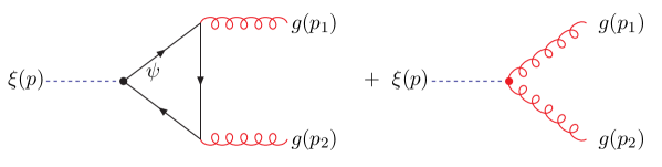
Figure 2: Feynman diagrams for the 3-point 1PI amplitude of axion ($\xi$) and $SU(N_{c})$ gauge bosons ($g$). The fermion loop involves either the derivative couplings $c_{\psi_{i}}$ or the non-derivative coupling $c_{\mu}$.

Although we literally call $c_{g}$ and $c_{\mu}$ non-derivative couplings, they can be regarded as derivative couplings in perturbation theory since $G^{a}_{\mu\nu}\tilde{G}^{a\mu\nu}$ is a total divergence and $c_{\mu}$ can be rotated away into $c_{g}$ and $c_{\psi,\chi}$ by an appropriate $\xi$-dependent field redefinition (97). As a result, all perturbative amplitudes induced by the axion couplings $c_{g},c_{\mu}$ and $c_{\psi,\chi}$ are vanishing in the limit when the external axion momentum $p$ becomes zero. This can be easily understood by the continuous PQ symmetry

$$U(1)_{PQ}:\quad\xi\rightarrow\xi+c\,M_{\xi},\quad\psi\chi\rightarrow e^{-icc_{\mu}}\psi\chi\quad(c=\mbox{constant}),$$ (108)

which is an exact symmetry in perturbation theory in our case.

Of course, the above PQ symmetry can be explicitly broken by the $U(1)_{PQ}\times[SU(N_{c})]^{2}$ anomaly through non-perturbative effects such as the $SU(N_{c})$ instantons with

$$\int d^{4}x\,G^{a}_{\mu\nu}\tilde{G}^{a\mu\nu}\neq 0,$$ (109)

and also possibly by non-perturbative quantum gravity effects. Including such nonperturbative $SU(N_{c})$ dynamics, $c_{g}$ and $c_{\mu}$, more precisely the reparameterization-invariant combination $c_{g}-c_{\mu}$, can be regarded as genuine non-derivative coupling which can generate a non-trivial axion potential. To have a small parameter which allows a systematic expansion of the generated axion potential, let us assume that $\mu/\Lambda_{SU(N_{c})}\ll 1$. Then, at scales around $\Lambda_{SU(N_{c})}$, the light fermions $\psi,\chi$ form a bilinear condensation which can be parametrized as

$$\langle\psi\chi\rangle=\Lambda_{\psi}^{3}e^{i\eta/f_{\eta}},$$ (110)

where $\eta$ is a composite meson and $\Lambda_{\psi}\sim f_{\eta}\sim\Lambda_{SU(N_{c})}$. The behavior (98) of axion couplings under the fermion field redefinition (97) implies that the meson potential should be invariant under the following spurion transformation of the field and parameters:

$$\hskip 28.45274pt\frac{\eta}{f_{\eta}}\,\to\,\frac{\eta}{f_{\eta}}+(x_{\psi}+x_{\chi})\frac{\xi}{M_{\xi}},$$

$$c_{g}\,\to\,c_{g}+x_{\psi}+x_{\chi},\quad c_{\mu}\,\to\,c_{\mu}+x_{\psi}+x_{\chi}.$$ (111)

This suggests that

$$V(\xi,\eta)=U\Big{(}\frac{\eta}{f_{\eta}}+c_{g}\frac{\xi}{M_{\xi}}\Big{)}-\mu\Lambda_{\psi}^{3}\cos\Big{(}\frac{\eta}{f_{\eta}}-c_{\mu}\frac{\xi}{M_{\xi}}\Big{)}+{\cal O}(\mu^{2}\Lambda_{SU(N_{c})}^{2}),$$ (112)

where $U(\theta)={\cal O}(\Lambda_{SU(N_{c})}^{4})$ is a periodic function of $\theta$ which has a global minimum at $\theta=0$. Note that the precise form of $U(\theta)$ depends on the details of non-perturbative $SU(N_{c})$ dynamics, while the next term is unambiguously determined to be a simple cosine function. Without knowing the detailed form of $U(\theta)$, we can integrate out $\eta$ by minimizing $U(\theta)$ ($\theta\approx 0$), which results in

$$\frac{\eta}{f_{\eta}}=-c_{g}\frac{\xi}{M_{\xi}}+{\cal O}\Big{(}\frac{\mu}{\Lambda_{SU(N_{c})}}\Big{)}.$$ (113)

Inserting this solution to the potential (112), one finds the axion effective potential is given by

$$V_{\rm eff}(\xi)=-\mu\Lambda_{SU(N_{c})}^{3}\cos\Big{(}(c_{g}-c_{\mu})\frac{\xi}{M_{\xi}}\Big{)}+{\cal O}(\mu^{2}\Lambda_{SU(N_{c})}^{2}).$$ (114)

Since the basis-independent $c_{g}-c_{\mu}$ has an integer value, this axion potential is manifestly consistent with the axion periodicity $\xi\equiv\xi+2\pi M_{\xi}$ regardless of the value of $c_{g}$ which can be highly suppressed in some particular field basis.

3.2 Models of multiple axions with clockwork-type $U(1)$ gauge charges

Our next example is a model of $N$ axions $\vec{\theta}=(\theta^{1},\theta^{2},\cdots,\theta^{N})$ which have the Stückelberg mixing with $(N-1)$ $U(1)$ gauge bosons $A_{\mu}^{\alpha}$ ($\alpha=1,2,...,N-1$). The $U(1)$ gauge charges of $\vec{\theta}$ take the clockwork form Bonnefoy:2018ibr :

$$\vec{k}_{1}=(1,-q,0,0,\cdots,0),\ \vec{k}_{2}=(0,1,-q,\cdots,0),\ \cdots,\ \vec{k}_{N-1}=(0,0,\cdots,1,-q)$$ (115)

for an integer $q>1$. Then the corresponding $\vec{\tilde{k}}$, $\vec{\ell}$ and $\vec{\tilde{\ell}}^{\alpha}$ are found to be

$$\hskip 56.9055pt\vec{\tilde{k}}=(q^{N-1},q^{N-2},\cdots,q,1),\quad\vec{\ell}=(0,0,\cdots,0,1),$$

$$\vec{\tilde{\ell}}^{1}=(1,0,\cdots,0,0),\quad\vec{\tilde{\ell}}^{2}=(q,1,\cdots,0,0),\quad\cdots,\quad\vec{\tilde{\ell}}^{N-1}=(q^{N-2},q^{N-3},\cdots,1,0).$$

For simplicity, we assume all $U(1)_{\alpha}$ gauge couplings are universal, $g_{\alpha}=g$, and take the most simple form of the axion kinetic metric:

$$G_{ij}=\delta_{ij}f^{2}.$$ (116)

Then the gauge boson mass matrix is given by

$$g^{2}M_{A}^{2}=g^{2}\sum_{ij}G_{ij}k^{i}k^{j}=g^{2}f^{2}\left(\begin{array}[]{ccccc}1+q^{2}&-q&0&\cdots&0\\ -q&1+q^{2}&-q&\cdots&0\\ \vdots&\vdots&\ddots&\vdots&-q\\ 0&0&\cdots&-q&1+q^{2}\end{array}\right),$$ (121)

which results in the mass eigenvalues

$$\left(M_{A}^{(n)}\right)^{2}=g^{2}f^{2}\left(1+q^{2}-2q\cos\frac{n\pi}{N}\right)\quad(n=1,2,\cdots,N-1).$$ (122)

As anticipated in the previous section, the axion decay constant of $\xi$, which is defined by the periodicity $\xi\equiv\xi+2\pi M_{\xi}$, is exponentially reduced as

$$M_{\xi}=\frac{1}{\sqrt{\sum_{ij}(G^{-1})^{ij}\tilde{k}_{i}\tilde{k}_{j}}}=\frac{f}{{||\tilde{k}||}}=\sqrt{\frac{q^{2}-1}{q^{2N}-1}}f\,\sim\,\frac{f}{q^{N-1}},$$ (123)

which is consistent with the behavior (74) in the limit $N\gg 1$ as the root mean square of the $U(1)$ charges is estimated as $(k^{i}_{r\alpha})_{\rm rms}\sim q/\sqrt{N}$.

However, having the field range $M_{\xi}\ll f$ does not mean that the couplings of $\xi$ are of the order of $1/M_{\xi}\gg 1/f$. The gauge-invariant axion $\xi$ interacts with other fields through the wavefunction mixing between $\xi$ and the original angular axions $\theta^{i}$. Then from the decomposition

$$\theta^{i}=\sum_{\alpha=1}^{N-1}k^{i}_{\alpha}\zeta^{\alpha}+\frac{q^{2}-1}{(q^{N}-q^{-N})q^{i}}\frac{\xi}{M_{\xi}}=\sum_{\alpha=1}^{N-1}k^{i}_{\alpha}\zeta^{\alpha}+\Big{(}\ell^{i}+\sum_{\alpha=1}^{N-1}\Gamma^{\alpha}\,k^{i}_{\alpha}\Big{)}\frac{\xi}{M_{\xi}},$$ (124)

where

$$\Gamma^{\alpha}=\frac{q^{\alpha}-q^{-\alpha}}{q^{N}-q^{-N}},$$ (125)

one immediately finds that the wavefunction mixing is given by

$$\langle\theta^{i}|\xi\rangle\,\sim\,\frac{1}{q^{i-1}}\,\frac{1}{f}.$$ (126)

As a consequence, unless one makes a $\xi$-dependent field redefinition which may change the characteristics of axion couplings, all couplings of $\xi$ are of the order of $1/f$ or smaller if the couplings of $\theta^{i}$ are of order unity or smaller.

To examine the axion couplings more explicitly, let us introduce $SU(N_{c})$ gauge fields $G^{a}_{\mu}$ and $N_{f}$ pairs of chiral fermions ($\psi_{I},\chi_{I}$) ($I=1,2,..,N_{f})$ whose $SU(N_{c})\times\prod_{\alpha}U(1)_{\alpha}$ gauge charges are given by

$$\psi_{I}=(N_{c},q_{\psi_{I}\alpha}),\quad\chi_{I}=(\bar{N}_{c},q_{\chi_{I}\alpha}).$$ (127)

Those gauge and matter fields can couple to $\theta^{i}$ as

$$\frac{1}{32\pi^{2}}\Big{(}\sum_{i}r_{i}\theta^{i}\Big{)}G^{a}_{\mu\nu}\tilde{G}^{a\mu\nu}-\Big{(}\sum_{I}\mu_{I}e^{i\sum_{i}n^{I}_{i}\theta^{i}}\psi_{I}\chi_{I}+{\rm h.c.}\Big{)}$$

$$\hskip 28.45274pt+\,\sum_{I,i}D_{\mu}\theta^{i}\Big{(}\kappa^{I}_{\psi i}\bar{\psi}_{I}\sigma^{\mu}\psi_{I}+\kappa^{I}_{\chi i}\bar{\chi}_{I}\sigma^{\mu}\chi_{I}\Big{)},$$ (128)

where the invariance under $\prod_{\alpha}U(1)_{\alpha}$ requires

$$\sum_{i}r_{i}k^{i}_{\alpha}=\sum_{I}(q_{\psi_{I}\alpha}+q_{\chi_{I}\alpha}),\quad\sum_{i}n^{I}_{i}k^{i}_{\alpha}=q_{\psi_{I}\alpha}+q_{\chi_{I}\alpha}.$$ (129)

Here for simplicity we consider only the flavour-diagonal axion couplings. After integrating out the massive $U(1)_{\alpha}$ gauge fields $A^{\alpha}_{\mu}-\partial_{\mu}\zeta^{\alpha}$, one finds the low energy couplings of $\xi$ given by

$$\frac{c_{g}}{32\pi^{2}}\frac{\xi}{M_{\xi}}G^{a\mu\nu}\tilde{G}^{a}_{\mu\nu}-\Big{(}\sum_{I}\mu_{I}e^{ic^{I}_{\mu}\xi/M_{\xi}}\psi_{I}\chi_{I}+{\rm h.c.}\Big{)}$$

$$\hskip 28.45274pt+\,\frac{\partial_{\mu}\xi}{M_{\xi}}\sum_{I}\left(c_{\psi}^{I}\bar{\psi}_{I}\sigma^{\mu}\psi_{I}+c_{\chi}^{I}\bar{\chi}_{I}\sigma^{\mu}\chi_{I}\right),$$ (130)

where

$$c_{g}=\frac{q^{2}-1}{q^{N}-q^{-N}}\sum_{i}\frac{r_{i}}{q^{i}},\qquad c_{\mu}^{I}=\frac{q^{2}-1}{q^{N}-q^{-N}}\sum_{i}\frac{n_{i}^{I}}{q^{i}},$$

$$c_{\psi}^{I}=\frac{q^{2}-1}{q^{N}-q^{-N}}\sum_{i}\frac{\kappa_{\psi i}^{I}}{q^{i}},\qquad c_{\chi}^{I}=\frac{q^{2}-1}{q^{N}-q^{-N}}\sum_{i}\frac{\kappa_{\chi i}^{I}}{q^{i}}.$$ (131)

Hence in this prescription, the effective axion couplings $c_{g},c_{\mu}^{I},c_{\psi}^{I}$ and $c_{\chi}^{I}$ are manifestly suppressed by $1/q^{N}\ll 1$ relative to the original axion couplings $r_{i},n_{i}^{I},\kappa_{\psi i}^{I},\kappa_{\chi i}^{I}$, and therefore all couplings of $\xi$ are of the order of $1/f\sim 1/q^{N-1}M_{\xi}$ or smaller as long as the original couplings of $\theta^{i}$ are of order unity or smaller. On the other hand, in the new field basis after the field redefinition (67), one finds

$$\hskip 56.9055ptc_{g}=\sum_{i}r_{i}\ell^{i}=r_{N},\quad c_{\mu}^{I}=\sum_{i}n^{I}_{i}\ell^{i}=n_{N}^{I},$$

$$c_{\psi}^{I}=\kappa_{\psi N}^{I}+\sum_{\alpha}\Gamma^{\alpha}(q_{\psi_{I}\alpha}+\sum_{i}\kappa_{\psi i}^{I}k^{i}_{\alpha}),\quad c_{\chi}^{I}=\kappa_{\chi N}^{I}+\Gamma^{\alpha}(q_{\chi_{I}\alpha}+\sum_{i}\kappa_{\chi i}^{IJ}k^{i}_{\alpha}),$$ (132)

so the couplings do not reveal a suppression by $1/q^{N}$. This means that the characteristic size of axion couplings is so different in the two different field bases. On the other hand, all physical consequences of the model should be independent of the choice of field basis. This indicates that one needs to be careful when examine the physical consequences of the axion couplings in the new field basis after the field redefinition (67) as there can be a fine cancellation among the contributions from different couplings.

To avoid a confusion due to the basis-dependent feature of the couplings, let us consider the basis-independent (reparameterization-invariant) combinations of axion couplings. Although we have introduced $3N_{f}+1$ axion couplings, all of their physical consequences can be described by the $N_{f}+1$ combinations of couplings:

$$\tilde{c}_{g}\equiv c_{g}-\sum_{I}c_{\mu}^{I}=\sum_{i}\Big{(}r_{i}-\sum_{I}n^{I}_{i}\Big{)}\ell^{i}=r_{N}-\sum_{I}n_{N}^{I},$$

$$\tilde{c}_{I}\equiv c^{I}_{\psi}+c^{I}_{\chi}+c_{\mu}^{I}=\frac{q^{2}-1}{q^{N}-q^{-N}}\sum_{i}\frac{\kappa_{\psi i}^{I}+\kappa_{\chi i}^{I}+n_{i}^{I}}{q^{i}},$$ (133)

which are invariant under the field redefinition

$$\psi_{I}\rightarrow e^{ix_{\psi_{I}}\xi/M_{\xi}}\psi_{I},\quad\chi_{I}\rightarrow e^{ix_{\chi_{I}}\xi/M_{\xi}}\chi_{I}.$$ (134)

For instance, the perturbative 3-point 1PI amplitude of $\xi$ to $SU(N_{c})$ gauge fields is given by

$$\hskip-17.07182pt{\cal A}_{\xi GG}=\frac{i\alpha_{s}}{2\pi M_{\xi}}\epsilon^{\mu\nu\rho\sigma}\epsilon_{1\mu}\epsilon_{2\nu}p_{1\rho}p_{2\sigma}\Big{[}\tilde{c}_{g}+\sum_{I}\tilde{c}_{I}F(p_{1},p_{2};\mu_{I})\Big{]},$$ (135)

where $p_{i\mu}$ and $\epsilon_{i}^{\mu}$ are the 4-momenta and polarization vectors of the two external gauge bosons and the loop function $F$ is given by (107), while the axion potential generated by non-perturbative $SU(N_{c})$ dynamics is determined by the integer-valued combination $\tilde{c}_{g}$ as

$$V_{\rm eff}\Big{(}\tilde{c}_{g}\frac{\xi}{M_{\xi}}\Big{)},$$ (136)

where $V_{\rm eff}(x)$ is a $2\pi$ periodic function of $x$, whose form is determined by more details of the model. Note that $\tilde{c}_{I}$ are continuous real numbers, while $\tilde{c}_{g}$ is integer-valued.

One might be puzzled about that the basis-independent combinations $\tilde{c}_{I}$ are suppressed by $1/q^{N}$ relative to the original axion couplings such as $\kappa_{\psi i}^{I},\kappa_{\chi i}^{I},n_{i}^{I}$, while there is no such suppression for $\tilde{c}_{g}$. This suggests that the model should involve a structure yielding an exponentially large number of ${\cal O}(q^{N})$ to have $\tilde{c}_{g}\neq 0$. Indeed the $U(1)_{\alpha}$ ($\alpha=1,2,..,N-1)$ gauge symmetries require such a structure and make it highly non-trivial to achieve $\tilde{c}_{g}\neq 0$. To see this, let us note that the gauge invariance condition (129) implies

$$\sum_{i}\Big{(}r_{i}-\sum_{I}n_{i}^{I}\Big{)}k^{i}_{\alpha}=0\quad\mbox{for all}\,\,\,\alpha=1,2,...,N-1,$$ (137)

and therefore $\vec{r}-\sum_{I}\vec{n}^{I}$ should be proportional to $\vec{\tilde{k}}$. Combined with $\tilde{c}_{g}=r_{N}-\sum_{I}n_{N}^{I}$ from (3.2), this determines $\vec{r}-\sum_{I}\vec{n}^{I}$ as

$$\vec{r}-\sum_{I}\vec{n}^{I}=\tilde{c}_{g}\vec{\tilde{k}}=\tilde{c}_{g}\,(q^{N-1},q^{N-2},\cdots,q,1).$$ (138)

Therefore $\tilde{c}_{g}$ can be non-zero in the limit $N\gg 1$ only when the model parameters $r_{i}$ and/or $\sum_{I}n^{I}_{i}$ are exponentially large as ${\cal O}(q^{N-i})$. In other word, $\xi$ can get a non-trivial potential from non-perturbative $SU(N_{c})$ dynamics only in the extreme case involving exponentially large parameter and/or exponentially many degrees of freedom Bonnefoy:2018ibr . This reflects that in the limit $N\gg 1$ the axion $\xi$ is so well protected by the $U(1)_{\alpha}$ ($\alpha=1,2,..,N-1$) gauge symmetries from getting a mass, so can be ultra-light in a natural manner.

As the above discussion suggests, one needs a non-trivial engineering to generate an effective potential of $\xi$. We close this subsection by providing one example of such engineering. Our example involves $N$ complex scalar fields $\phi_{P}$ with the $U(1)_{\alpha}$ gauge charges

$$q_{\phi_{P}\alpha}=\delta_{P\alpha}\quad(P=1,2,..,N;\,\,\,\alpha=1,2,..,N-1).$$ (139)

Although it is not essential for our discussion, to make the model simpler, we assume the discrete symmetry $\mathbb{Z}_{q+1}$ under which

$$\mathbb{Z}_{q+1}:\quad\theta^{i}\to\theta^{i}+(-1)^{i}\frac{2\pi}{q+1},\quad\phi_{P}\to e^{i(-1)^{P}(P+1)\frac{2\pi}{q+1}}\phi_{P}.$$ (140)

Then the scalar potentials of $\phi_{P}$ takes the form

$$V(\theta^{i},\phi_{I}) = \sum_{P}m_{P}^{2}|\phi_{P}|^{2}+\sum_{PQ}\lambda_{PQ}|\phi_{P}|^{2}|\phi_{Q}|^{2}$$

$$\hskip-56.9055pt-\,\epsilon_{1}e^{i(q+1)\theta^{1}}\phi_{1}^{*q+1}-\epsilon_{2}e^{i\theta^{2}}\phi_{1}^{q}\phi_{2}^{*}-\cdots-\epsilon_{N}e^{i\theta^{N}}\phi_{N-1}^{q}\phi_{N}^{*}-\epsilon_{N+1}\phi_{N}^{q+1}+{\rm h.c.}+...,$$

where the ellipsis denotes the higher-dimensional terms. Here we consider the case with $q=3$ or 2, but pretend that $q$ is a generic integer. After integrating out $\zeta^{\alpha}$ eaten by the $U(1)_{\alpha}$ gauge fields, the second line of the potential becomes

$$\hskip-5.69046pt-\epsilon_{1}e^{ib_{1}\xi/M_{\xi}}\phi_{1}^{*q+1}-\epsilon_{2}e^{ib_{2}\xi/M_{\xi}}\phi_{1}^{q}\phi_{2}^{*}-\cdots-\epsilon_{N}e^{ib_{N}\xi/M_{\xi}}\phi_{N-1}^{q}\phi_{N}^{*}-\epsilon_{N+1}\phi_{N}^{q+1}+{\rm h.c.},\quad$$ (141)

where

$$b_{1}=\frac{(q+1)(q^{2}-1)}{(q^{N}-q^{-N})q},\quad b_{2}=\frac{q^{2}-1}{(q^{N}-q^{-N})q^{2}},\quad\cdots,\quad b_{N}=\frac{q^{2}-1}{(q^{N}-q^{-N})q^{N}}.$$ (142)

One can easily arrange the model to have non-zero vacuum values of $\phi_{P}$, and then $\phi_{P}$ can be decomposed as

$$\phi_{P}(x)=\frac{1}{\sqrt{2}}\Big{(}v_{P}+h_{P}(x)\Big{)}e^{ia_{P}(x)/v_{P}},$$ (143)

where $v_{P}/\sqrt{2}=\langle\phi_{P}\rangle$ and $h_{P}$ denotes the radial fluctuation of $\phi_{P}$. Here we are interested in the limit that $\epsilon_{I}$ are small enough, so that the phase fields $a_{P}$ can be regarded as light pseudo-Goldstone bosons. Then the massive $h_{P}$ can be safely integrated out, while leaving the following effective potential of $a_{P}$ and $\xi$:

$$\hskip-19.91684ptV_{\rm eff}(\xi,a_{I}) = -\Lambda_{1}^{4}\cos\Big{(}(q+1)\frac{a_{1}}{v_{1}}-b_{1}\frac{\xi}{M_{\xi}}\Big{)}-\Lambda_{2}^{4}\cos\Big{(}q\frac{a_{1}}{v_{1}}-\frac{a_{2}}{v_{2}}+b_{2}\frac{\xi}{M_{\xi}}\Big{)}+\cdots$$ (144)

$$\hskip-14.22636pt-\,\Lambda_{N}^{4}\cos\Big{(}q\frac{a_{N-1}}{v_{N-1}}-\frac{a_{N}}{v_{N}}+b_{N}\frac{\xi}{M_{\xi}}\Big{)}-\Lambda_{N+1}^{4}\cos\Big{(}(q+1)\frac{a_{N}}{v_{N+1}}\Big{)},$$

where

$$\Lambda_{1}^{4}=\frac{\epsilon_{1}v_{1}^{q+1}}{2^{(q-1)/2}},~{}\Lambda_{2}^{4}=\frac{\epsilon_{2}v_{1}^{q}v_{2}}{2^{(q-1)/2}},~{}\cdots,~{}\Lambda_{N}^{4}=\frac{\epsilon_{N}v_{N-1}^{q}v_{N}}{2^{(q-1)/2}},~{}\Lambda_{N+1}^{4}=\frac{\epsilon_{N+1}v_{N}^{q+1}}{2^{(q-1)/2}}.$$ (145)

The above potential involves $N+1$ independent terms for the $N+1$ pseudo-Goldstone bosons involving $\xi$ and $a_{P}$, so can provide a non-trivial effective potential of $\xi$ which would be the lightest pseudo-Goldstone boson in the parameter limit $v_{P}\ll M_{\xi}$. In fact, the above potential of $N+1$ pseudo-Goldstone bosons reveal the clockwork structure studied before Choi:2014rja ; Choi:2015fiu ; Kaplan:2015fuy ; Giudice:2016yja . To proceed, let us first minimize the above potential except the first and last terms under the assumption that all $\Lambda_{I}$ ($I=2,3,..,N$) are comparable to each other. This results in the following $\xi$-dependent vacuum values of $a_{I}$ ($I=1,2,..,N-1$):

$$\frac{a_{1}}{v_{1}}=\frac{1}{q}\left(\frac{a_{2}}{v_{2}}-\frac{b_{2}\xi}{M_{\xi}}\right),~{}\frac{a_{2}}{v_{2}}=\frac{1}{q}\left(\frac{a_{3}}{v_{3}}-\frac{b_{3}\xi}{M_{\xi}}\right),~{}\cdots,\quad\frac{a_{N-1}}{v_{N-1}}=\frac{1}{q}\left(\frac{a_{N}}{v_{N}}-\frac{b_{N}\xi}{M_{\xi}}\right).$$ (146)

Inserting these to (144), we get the effective potential of $\xi$ and $a_{N}$, which is given by

$$V_{\rm eff}(\xi,a_{N})=-\Lambda_{1}^{4}\cos\left(\frac{q+1}{q^{N-1}}\Big{(}\frac{a_{N}}{v_{N}}-\frac{\xi}{M_{\xi}}\Big{)}\right)-\Lambda_{N+1}^{4}\cos\Big{(}(q+1)\frac{a_{N}}{v_{N}}\Big{)}.$$ (147)

If $\Lambda_{1}\sim\Lambda_{N+1}$, $a_{N}$ gets a mass dominantly from the second term with a vanishing vacuum value, which would result in

$$V_{\rm eff}(\xi) \simeq -\Lambda_{1}^{4}\cos\Big{(}\frac{q+1}{q^{N-1}}\frac{\xi}{M_{\xi}}\Big{)}.$$ (148)

In this case the scalar potential (141) not only provides a non-trivial effective potential of $\xi$, but also enlarges the axion field range from $M_{\xi}$ to $q^{N-1}M_{\xi}$ through the clockwork mechanism Choi:2014rja ; Choi:2015fiu ; Kaplan:2015fuy ; Giudice:2016yja . Yet there exists a parameter limit where a non-trivial potential of $\xi$ is generated while keeping the axion field range as $M_{\xi}$. If $\Lambda_{N+1}^{2}/\Lambda_{1}^{2}\ll 1/q^{N-1}$, $a_{N}$ gets a mass dominantly from the first term of (147) with the $\xi$-dependent vacuum value

$$\frac{a_{N}}{v_{N}}=\frac{\xi}{M_{\xi}},$$ (149)

yielding the effective potential

$$V_{\rm eff}(\xi) \simeq -\Lambda_{N+1}^{4}\cos\Big{(}(q+1)\frac{\xi}{M_{\xi}}\Big{)}$$ (150)

without changing the field range of $\xi$. At any rate, our example shows again that $\xi$ is so well protected by $\prod_{\alpha}U(1)_{\alpha}$, so it requires a highly non-trivial engineering to generate an effective potential of $\xi$ in the limit $N\gg 1$.

4 Conclusion

Stückelberg mixing between axions and $U(1)$ gauge bosons can result in a variety of interesting consequences in low energy axion physics. In this paper, we studied those consequences in a general framework which can be applied for many different situations. More specifically we derived the field range of the gauge-invariant axion combination $\xi$ for generic form of axion kinetic metric and $U(1)$ gauge charges, and examined the low energy axion couplings to matter and gauge fields in models with Stückelberg mixing, as well as some of their physical consequences. Stückelberg mixing typically reduces the field range of $\xi$ compared to the mass scales introduced in the UV theory. In particular, for the case of Stückelberg mixing between $N$ axions and $(N-1)$ $U(1)$ gauge bosons in the limit $N\gg 1$, the axion field range can be exponentially reduced relative to the mass scales in the UV theory. As is well known, axion couplings in the effective lagrangian vary under the axion-dependent field redefinition of matter fields, so depend on the choice of the matter field basis. It is noted that in some parameter limit of Stückelberg mixing the axion couplings to matter and gauge fields can have hierarchically different size in different field bases, and then one needs to consider the basis-independent (reparameterization-invariant) combination of couplings rather than focusing on a specific basis-dependent coupling to see the physical consequence of the model.

- (1) For reviews on axions, see for instance J. E. Kim and G. Carosi, Rev. Mod. Phys. 82, 557 (2010) [arXiv:0807.3125 [hep-ph]]; M. Kawasaki and K. Nakayama, Ann. Rev. Nucl. Part. Sci. 63, 69 (2013) [arXiv:1301.1123 [hep-ph]]; D. J. E. Marsh, Phys. Rept. 643, 1 (2016) [arXiv:1510.07633 [astro-ph.CO]].
- (2) K. Freese, J. A. Frieman and A. V. Olinto, Phys. Rev. Lett. 65, 3233 (1990).
- (3) K. Choi, Phys. Rev. D 62, 043509 (2000) [hep-ph/9902292].
- (4) P. W. Graham, D. E. Kaplan and S. Rajendran, Phys. Rev. Lett. 115, no. 22, 221801 (2015) [arXiv:1504.07551 [hep-ph]].
- (5) E. Witten, Phys. Lett. 149B, 351 (1984).
- (6) K. Choi and J. E. Kim, Phys. Lett. 154B, 393 (1985) Erratum: [Phys. Lett. 156B, 452 (1985)]; K. Choi and J. E. Kim, Phys. Lett. 165B, 71 (1985).
- (7) P. Svrcek and E. Witten, JHEP 0606, 051 (2006) [hep-th/0605206].
- (8) A. Arvanitaki, S. Dimopoulos, S. Dubovsky, N. Kaloper and J. March-Russell, Phys. Rev. D 81, 123530 (2010) [arXiv:0905.4720 [hep-th]].
- (9) N. Arkani-Hamed, L. Motl, A. Nicolis and C. Vafa, JHEP 0706, 060 (2007) [hep-th/0601001].
- (10) N. Arkani-Hamed, H. C. Cheng, P. Creminelli and L. Randall, Phys. Rev. Lett. 90, 221302 (2003) [hep-th/0301218].
- (11) J. E. Kim, H. P. Nilles and M. Peloso, JCAP 0501, 005 (2005) [hep-ph/0409138].
- (12) S. Dimopoulos, S. Kachru, J. McGreevy and J. G. Wacker, JCAP 0808, 003 (2008) [hep-th/0507205].
- (13) E. Silverstein and A. Westphal, Phys. Rev. D 78, 106003 (2008) [arXiv:0803.3085 [hep-th]].
- (14) N. Kaloper and L. Sorbo, Phys. Rev. Lett. 102, 121301 (2009) [arXiv:0811.1989 [hep-th]].
- (15) F. Marchesano, G. Shiu and A. M. Uranga, JHEP 1409, 184 (2014) [arXiv:1404.3040 [hep-th]].
- (16) K. Choi, H. Kim and S. Yun, Phys. Rev. D 90, 023545 (2014) [arXiv:1404.6209 [hep-th]].
- (17) T. Higaki and F. Takahashi, JHEP 1407, 074 (2014) [arXiv:1404.6923 [hep-th]].
- (18) T. C. Bachlechner, M. Dias, J. Frazer and L. McAllister, Phys. Rev. D 91, no. 2, 023520 (2015) [arXiv:1404.7496 [hep-th]].
- (19) I. Ben-Dayan, F. G. Pedro and A. Westphal, Phys. Rev. Lett. 113, 261301 (2014) [arXiv:1404.7773 [hep-th]].
- (20) T. Rudelius, JCAP 1504, 049 (2015) [arXiv:1409.5793 [hep-th]].
- (21) T. C. Bachlechner, C. Long and L. McAllister, JHEP 1512, 042 (2015) [arXiv:1412.1093 [hep-th]].
- (22) A. de la Fuente, P. Saraswat and R. Sundrum, Phys. Rev. Lett. 114, no. 15, 151303 (2015) [arXiv:1412.3457 [hep-th]].
- (23) G. Shiu, W. Staessens and F. Ye, Phys. Rev. Lett. 115, 181601 (2015) [arXiv:1503.01015 [hep-th]].
- (24) G. Shiu, W. Staessens and F. Ye, JHEP 1506, 026 (2015) [arXiv:1503.02965 [hep-th]].
- (25) M. Montero, A. M. Uranga and I. Valenzuela, JHEP 1508, 032 (2015) [arXiv:1503.03886 [hep-th]].
- (26) J. Brown, W. Cottrell, G. Shiu and P. Soler, JHEP 1510, 023 (2015) [arXiv:1503.04783 [hep-th]].
- (27) A. Hebecker, P. Mangat, F. Rompineve and L. T. Witkowski, Phys. Lett. B 748, 455 (2015) [arXiv:1503.07912 [hep-th]].
- (28) D. Junghans, JHEP 1602, 128 (2016) [arXiv:1504.03566 [hep-th]].
- (29) B. Heidenreich, M. Reece and T. Rudelius, JHEP 1512, 108 (2015) [arXiv:1506.03447 [hep-th]].
- (30) K. Choi and S. H. Im, JHEP 1601, 149 (2016) [arXiv:1511.00132 [hep-ph]].
- (31) D. E. Kaplan and R. Rattazzi, Phys. Rev. D 93, no. 8, 085007 (2016) [arXiv:1511.01827 [hep-ph]].
- (32) G. F. Giudice and M. McCullough, JHEP 1702, 036 (2017) [arXiv:1610.07962 [hep-ph]].
- (33) T. C. Bachlechner, K. Eckerle, O. Janssen and M. Kleban, Phys. Rev. D 98, no. 6, 061301 (2018) [arXiv:1703.00453 [hep-th]].
- (34) T. C. Bachlechner, K. Eckerle, O. Janssen and M. Kleban, JHEP 1711, 036 (2017) [arXiv:1709.01080 [hep-th]].
- (35) G. Shiu and W. Staessens, JHEP 1810, 085 (2018) [arXiv:1807.00888 [hep-th]].
- (36) N. Fonseca, B. von Harling, L. de Lima and C. S. Machado, arXiv:1906.10193 [hep-ph].
- (37) Q. Bonnefoy, E. Dudas and S. Pokorski, Eur. Phys. J. C 79, no. 1, 31 (2019) [arXiv:1804.01112 [hep-ph]].