Quantum exceptional points of non-Hermitian Hamiltonians and Liouvillians:
The effects of quantum jumps

Abstract

Exceptional points (EPs) correspond to degeneracies of open systems. These are attracting much interest in optics, optoelectronics, plasmonics, and condensed matter physics. In the classical and semiclassical approaches, Hamiltonian EPs (HEPs) are usually defined as degeneracies of non-Hermitian Hamiltonians such that at least two eigenfrequencies are identical and the corresponding eigenstates coalesce. HEPs result from continuous, mostly slow, nonunitary evolution without quantum jumps. Clearly, quantum jumps should be included in a fully quantum approach to make it equivalent to, e.g., the Lindblad master-equation approach. Thus, we suggest to define EPs via degeneracies of a Liouvillian superoperator (including the full Lindbladian term, LEPs), and we clarify the relations between HEPs and LEPs. We prove two main theorems: Theorem 1 proves that, in the quantum limit, LEPs and HEPs must have essentially different properties. Theorem 2 dictates a condition under which, in the “semiclassical” limit, LEPs and HEPs recover the same properties. In particular, we show the validity of Theorem 1 studying systems which have (1) an LEP but no HEPs, and (2) both LEPs and HEPs but for shifted parameters. As for Theorem 2, (3) we show that these two types of EPs become essentially equivalent in the semiclassical limit. We introduce a series of mathematical techniques to unveil analogies and differences between the HEPs and LEPs. We analytically compare LEPs and HEPs for some quantum and semiclassical prototype models with loss and gain.

I Introduction

Exceptional points (EPs) are attracting increasing interest, both theoretically and experimentally, in diverse fields including optics, condensed-matter physics, plasmonics, and even electronics. For example, as summarized in very recent reviews Özdemir et al. (2019); Miri and Alù (2019), EPs are considered for novel enhanced sensing apparatus and are relevant to describe dynamical phase transitions and in the characterization of topological phases of matter in open systems. This research in EPs was triggered two decades ago by the introduction of non-Hermitian quantum mechanics Bender and Boettcher (1998) or, more specifically, by the discovery of non-Hermitian Hamiltonians (NHHs) with real eigenvalues for parity-time-symmetric nonconservative systems Christodoulides and Yang (2018). An EP of an NHH (which for short we refer to as a Hamiltonian EP or an HEP) refers to the NHH degeneracies where two (or more) eigenfrequencies coincide and the corresponding eigenstates coalesce. Since an EP corresponds to a nondiagonalizable operator, standard Hermitian Hamiltonians cannot display any EP. It is the nonunitary effect of the environment that induces the emergence of EPs. Such points can be found, e.g., by balancing the attenuation, amplification, gain saturation, as well as various Hamiltonian coupling strengths of an open system (as experimentally shown in, e.g., Refs. Peng et al. (2014a); Gao et al. (2015); Naghiloo et al. (2019)).

The dynamics of an open quantum system is characterized by the presence of dissipative terms describing the progressive loss of energy, coherence, and information into the environment. Under very general hypotheses, the equation of motion can be captured by a Lindblad form consisting of a Hermitian Hamiltonian part, describing the coherent evolution of the system, and a non-Hermitian part, the so-called Lindblad dissipators. These Lindblad dissipators admit a fascinating interpretation in terms of quantum maps and measurement theory Wiseman and Milburn (2010); Haroche and Raimond (2006); Barnett (2009); Paris (2012), and can be divided into two parts: The first one represents a coherent nonunitary dissipation of the system, transforming the Hamiltonian in an NHH. The second one describes quantum jumps, which are the effect of a continuous measurement performed by the environment on the system.

The instantaneous switching between energy levels in quantum systems, caused by quantum jumps, is pivotal to correctly describe microscopic open systems. These quantum jumps lay at the foundation of quantum physics, being necessary to obtain a consistent measurement theory once the environment is taken into account Wiseman and Milburn (2010); Daley (2014); Carmichael (1999, 2007). Quantum jumps have been observed in countless experiments, including ionic Nagourney et al. (1986); Sauter et al. (1986); Bergquist et al. (1986), atomic Peil and Gabrielse (1999); Basché et al. (1995); Gleyzes et al. (2007); Guerlin et al. (2007); Deléglise et al. (2008); Sayrin et al. (2011), solid-state Jelezko et al. (2002); Neumann et al. (2010); Robledo et al. (2011), and superconducting circuit setups Vijay et al. (2011); Hatridge et al. (2013); Sun et al. (2014); Ofek et al. (2016); Minev et al. (2019). Hence, to correctly describe exceptional points of quantum systems, one must consider quantum jumps.

The vast majority of studies on EPs, especially in the context of parity-time-symmetric systems, have been limited to classical or semiclassical models where quantum jumps were ignored (e.g., Jing et al. (2014); Peng et al. (2014a)). Indeed, the standard calculation of EPs (i.e., HEPs) is based on finding degeneracies of non-Hermitian Hamiltonians. Thus, such approaches cannot be completely equivalent to the standard Lindblad master equation, as clearly seen by referring to the quantum trajectory method (also known as the quantum jump method) Haroche and Raimond (2006); Plenio and Knight (1998); Carmichael (1993); Dalibard et al. (1992); Mølmer et al. (1993).

The time evolution of a system obeying a Lindblad master equation is captured by a Liouvillian superoperator. Since the Liouvillian is a non-Hermitian matrix, it too can exhibit EPs Lidar ; Albert and Jiang (2014); Minganti et al. (2018); Macieszczak et al. (2016); Sarandy and Lidar (2005); Hatano (2019); Prosen (2010); van Caspel et al. (2019). Liouvillian EPs (LEPs) are defined via degeneracies of Liouvillians (including the full Lindbladian terms), i.e., when two (or more) eigenfrequencies and the corresponding eigenstates of a given Liouvillian coalesce. The physical meaning of LEPs and its relation to HEPs, however, are crucial to correctly understand HEPs in the quantum case.

The main objective of this paper is to point out the similarities and differences between HEPs and LEPs. To do that, we introduce the Liouvillian without quantum jumps $\mathcal{L}^{\prime}$, as well as the exceptional points resulting from a Liouvillian without quantum jumps (LEP’s). We prove the severe limits of the NHH approach to correctly capture the full quantum regime, and we demonstrate how quantum jumps can also affect the semiclassical dynamics of a system. In this regard, we provide a procedure to generalize the semiclassical HEPs to include quantum jumps. We prove theorems about the general properties of HEPs and LEPs, showing their equivalence in the semiclassical regime and some fundamental differences in the quantum regime. We also compare the basic properties of HEPs and LEPs. By introducing a series of mathematical techniques, we unveil analogies and differences between the HEPs and LEPs. We demonstrate these similarities and discrepancies on three prototype examples.

This paper is organized as follows: In Sec. II, we discuss the semiclassical limit, how in this limit the NHH stems from a Liouvillian and how, vice versa, a Liouvillian is the minimal extension of an NHH to the quantum regime. In Sec. III we provide the main results of this paper, i.e., Theorems 1 and 2, which prove some relations between the spectra of an NHH and the corresponding Liouvillian. In Secs. IV, V, and VI, we demonstrate the validity of the theorems on three examples. Finally, in the Appendix A we recall, for pedagogical reasons, some useful properties of superoperators.

In the main article we will use all the previously introduced abbreviations. In Table 1 we concisely list them to facilitate the reading of the article.

Full Name	Abbreviation
Non-Hermitian Hamiltonian	NHH
Liouvillian	$\mathcal{L}$
Liouvillian without quantum jumps	$\mathcal{L}^{\prime}$
Exceptional point	EP
Hamiltonian exceptional point	HEP
Liouvillian exceptional point	LEP
LEP without quantum jumps	LEP’

Table 1: List of abbreviation used in the main article, and corresponding full names.

II Non-Hermitian Hamiltonians, Liouvillians, and their semiclassical approximation

In this section, we introduce in detail the concept of non-Hermitian Hamiltonian (NHH) and Liouvillian stemming from the Lindblad master equation. In particular, we explain that the semiclassical limit of a Liouvillian is an NHH, and we provide a physical interpretation of the resulting effective Hamiltonian. Vice versa, we demonstrate that the Lindblad master equation is a minimal quantum map that extends the behavior of a non-Hermitian Hamiltonian to its “quantum” limit.

Before proceeding further, let us clarify the usage of the term semiclassical limit to be applied in this paper. In the literature, the “semiclassical approximation” is loosely and widely used with different meanings Arndt (2009). Thus, the semiclassical regime can be defined in various ways depending on its physical context Schlosshauer (2007). These meanings include:
(1) In the traditional interpretation of nonrelativistic quantum mechanics, the semiclassical limit corresponds to assuming $\hbar\to 0$, transforming operators into variables, and replacing the Hilbert space tensor-product structure with the direct sum of classical phase spaces.
(2) One can also refer to the semiclassical regime of a quantum system that can be well approximated by a classical model for high quantum numbers. A classical example can be provided by the coherent-state approximation of the electromagnetic field in quantum optics Walls and Milburn (1994), where the evolution of a state inside a cavity is well captured by the evolution of a complex number. Moreover, this is often the case when discussing room-temperature condensed-matter systems for which quantum characteristics are well captured by phenomenological classical theories (e.g., the Drude scattering theory for electrons or the Johnson-Nyquist noise).
(3) Another meaning of the semiclassical approximation regards composite systems, that is, when the system can be described as a classical subsystem interacting with a quantum one. For example, the standard optical Bloch equations Haroche and Raimond (2006); Carmichael (1999) describe a quantum two-level system coupled to a classical electromagnetic field.
(4) Moreover, one can consider that, during the dissipative evolution of a quantum system, different physical properties evolve at different rates, dictating a passage from the quantum to the semiclassical regime. In particular, one can introduce the pointer states of dissipation as the classical states emerging from a prolonged interaction with a complex environment Zurek (2003).
(5) In the literature about EPs, the effects of quantum noise are neglected by claiming that the model is semiclassical. Similarly, in the present discussion, the semiclassical limit means that we neglect the action of quantum jumps without taking much care of which of the previous four criteria can be applied.

Specifically, we will have a well-defined semiclassical regime (or semiclassical limit) of the Markovian dynamics of a given quantum system if all (or at least some nontrivial) EPs of a non-Hermitian Hamiltonian are effectively the same as those of a corresponding Liouvillian in a Lindblad master equation with quantum jumps terms. We stress that all the EPs of a non-Hermitian Hamiltonian (i.e., HEPs) are exactly the same as the EPs of a Liouvillian without quantum jump terms (LEP’s).

II.1 The Liouvillian and its semiclassical limit

The time evolution of an open quantum system weakly interacting with a Markovian (i.e., memoryless) environment can be expressed using the so-called Lindblad master equation Carmichael (1999); Breuer and Petruccione (2007); Haroche and Raimond (2006); Walls and Milburn (1994); Gardiner and Zoller (2004); Wiseman and Milburn (2010) (hereafter, we set $\hbar=1$):

$$\frac{\partial\hat{\rho}(t)}{\partial t}=\mathcal{L}\hat{\rho}(t)=-i\left[\hat{H},\hat{\rho}(t)\right]+\sum_{\mu}\mathcal{D}[\hat{\Gamma}_{\mu}]\hat{\rho}(t),$$ (1)

where $\hat{\rho}(t)$ is the density matrix of a system at a time $t$ and $\mathcal{D}[\hat{\Gamma}_{\mu}]$ are the dissipators associated with the jump operators $\hat{\Gamma}_{\mu}$, while $\mathcal{L}$ is the so-called Liouvillian superoperator (for a detailed discussion about superoperators, see Appendix A). The density matrix $\hat{\rho}(t)$ can describe both pure states $\ket{\phi}\bra{\phi}$ and probabilistic mixture $\sum_{i}p_{i}\ket{\phi_{i}}\bra{\phi_{i}}$Cohen-Tannoudji et al. (1991); Carmichael (1999); Gardiner and Zoller (2004); Haroche and Raimond (2006); Paris (2012); Rivas and Huelga (2011). Each dissipator is defined by the Lindbladian

$$\mathcal{D}[\hat{\Gamma}_{\mu}]\hat{\rho}(t)=\hat{\Gamma}_{\mu}\hat{\rho}(t)\hat{\Gamma}_{\mu}^{\dagger}-\frac{\hat{\Gamma}_{\mu}^{\dagger}\hat{\Gamma}_{\mu}}{2}\hat{\rho}(t)-\hat{\rho}(t)\frac{\hat{\Gamma}_{\mu}^{\dagger}\hat{\Gamma}_{\mu}}{2}.$$ (2)

The Lindblad master equation admits a very appealing interpretation as the time evolution of a system which is continuously monitored by an environment Haroche and Raimond (2006). In this regard, the effect of $\mathcal{D}[\hat{\Gamma}_{\mu}]$ on the density matrix $\hat{\rho}(t)$ can be split into two parts Wiseman and Milburn (2010): the continuous nonunitary dissipation terms, $\hat{\Gamma}_{\mu}^{\dagger}\hat{\Gamma}_{\mu}\hat{\rho}(t)+\hat{\rho}(t)\hat{\Gamma}_{\mu}^{\dagger}\hat{\Gamma}_{\mu}$, and the quantum jump terms,

$$\mathcal{J}[\hat{\Gamma}_{\mu}]\hat{\rho}(t)=\hat{\Gamma}_{\mu}\hat{\rho}(t)\hat{\Gamma}_{\mu}^{\dagger}.$$ (3)

The dissipation describes the continuous losses of energy, information, and coherence of the system into the environment, while the quantum jumps describe the effect of the measurement on the state of the system Barnett (2009); Wiseman and Milburn (2010); Haroche and Raimond (2006). We label the term $\mathcal{J}[\hat{\Gamma}_{\mu}]$ a quantum jump since in a quantum trajectory approach (i.e., a wave-function Monte Carlo method) Mølmer et al. (1993); Dalibard et al. (1992); Daley (2014); Carmichael (1993), those are the terms responsible for the abrupt stochastic change of the wave function. In this regard, given a Lindblad master equation describing the microscopic physics of a given system, it is easy to obtain the corresponding “semiclassical limit” by neglecting the effect of quantum jumps, and introducing an effective NHH of the form

$$\hat{H}_{\rm eff}=\hat{H}-i\sum\hat{\Gamma}_{\mu}^{\dagger}\hat{\Gamma}_{\mu}/2.$$ (4)

An equation of motion for a generic density matrix $\hat{\rho}(t)$ thus becomes:

$$\frac{\partial\hat{\rho}(t)}{\partial t}=\mathcal{L}^{\prime}\hat{\rho}(t)=-i\left(\hat{H}_{\rm eff}\hat{\rho}(t)-\hat{\rho}(t)\hat{H}_{\rm eff}^{\dagger}\right),$$ (5)

where we have introduced the Liouvillian without quantum jumps $\mathcal{L}^{\prime}$. Indeed, in this evolution, one assumes that the effect of the jump operators $\hat{\Gamma}_{\mu}$ is negligible due to the semiclassical nature of the system state. We stress that this condition requires that not only the steady state but also all the states explored by the Liouvillian dynamics can be well described via a non-Hermitian Hamiltonian. Indeed, as it will be detailed in Sec. III.3, the LEPs capture the dynamical properties of a system relaxing towards its steady state and as such cannot be captured by the properties of the steady state alone.

We note that the master equation in Eq. (1) can be rewritten in terms of $\hat{H}_{\rm eff}$ as follows:

$$\frac{\partial\hat{\rho}(t)}{\partial t}=\mathcal{L}\hat{\rho}(t)=-i\left(\hat{H}_{\rm eff}\hat{\rho}(t)-\hat{\rho}(t)\hat{H}_{\rm eff}^{\dagger}\right)+\sum_{\mu}\hat{\Gamma}_{\mu}\hat{\rho}(t)\hat{\Gamma}_{\mu}^{\dagger}.$$ (6)

Thus, it is clear that given a non-Hermitian Hamiltonian $\hat{H}_{\rm eff}$, together with the quantum jump terms $\hat{\Gamma}_{\mu}\hat{\rho}(t)\hat{\Gamma}_{\mu}^{\dagger}$ in Eq. (6), one can fully describe the quantum dynamics of a dissipative system within the Lindblad formalism. However, a natural way to calculate the EPs of a non-Hermitian Hamiltonian with the quantum jump terms requires the use of a superoperator rather than the operator $\hat{H}_{\rm eff}$ (see also Appendix A). This is because the quantum jump operators are on the left- and right-hand sides of a density matrix $\hat{\rho}(t)$ in the term $\hat{\Gamma}_{\mu}\hat{\rho}(t)\hat{\Gamma}_{\mu}^{\dagger}$. Such a superoperator is actually the Liouvillian $\mathcal{L}$ studied here.

Finally, $\hat{H}_{\rm eff}$ naturally emerges when discussing quantum trajectories and postselection. Quantum trajectories describe a system whose environment is continuously and perfectly probed Mølmer et al. (1993); Haroche and Raimond (2006); Carmichael (2007); Wiseman and Milburn (2010); Daley (2014). In this formalism, the system state is captured by a stochastic wave function $\ket{\psi(t)}$. In a counting trajectory, when no quantum jump happens, $\ket{\psi(t)}$ evolves smoothly according to $\hat{H}_{\rm eff}$. Otherwise, the wave function abruptly changes under the action of a jump operator, $\hat{\Gamma}_{\mu}\ket{\psi(t)}$ Wiseman and Milburn (2010). The Lindblad master equation describes the average over infinite quantum trajectories, i.e., infinitely many experiments. In some of these experiments, a quantum jump took place. If, instead, one considers only those trajectories where no quantum jumps happened, the average over many different trajectories would be described by $\mathcal{L}^{\prime}$. In this regard, to access the NHH in its quantum limit, one can use post-selection techniques, as done in Ref. Naghiloo et al. (2019).

II.2 Making sense of non-Hermitian Hamiltonians
in the quantum limit

We try now to reconcile the concept of NHHs with that of a quantum map.

Let us consider the following NHH:

$$\hat{H}_{\rm eff}=\hat{H}+\hat{A},$$ (7)

where we introduce the Hermitian operator $\hat{H}=(\hat{H}_{\rm eff}+\hat{H}^{\dagger}_{\rm eff})/2$ and the anti-Hermitian one $\hat{A}=(\hat{H}_{\rm eff}-\hat{H}^{\dagger}_{\rm eff})/2$. One can prove that the most general form of a linear, Hermiticity- and trace-preserving, and completely positive quantum map describing the time evolution of the density matrix $\hat{\rho}(t)$ is a superoperator $\mathcal{M}$ Haroche and Raimond (2006); Barnett (2009); Paris (2012), defined by

$$\hat{\rho}(t+\tau)=\mathcal{M}\hat{\rho}(t)=\sum_{\mu}\hat{M}_{\mu}\hat{\rho}(t)\hat{M}_{\mu}^{\dagger}\quad{\rm and}\quad\sum_{\mu}\hat{M}^{\dagger}_{\mu}\hat{M}_{\mu}=\mathds{1},$$ (8)

where $\mathcal{M}$ are the Kraus operators. Since this NHH captures well the dynamics of the system in its semiclassical limit, the time evolution of a generic density matrix $\hat{\rho}(t)$ under such an NHH is

$$\begin{split}\hat{\rho}(t+\tau)&=\hat{\rho}(t)-i\tau\left(\hat{H}_{\rm eff}\hat{\rho}(t)-\hat{\rho}(t)\hat{H}^{\dagger}_{\rm eff}\right)+\mathcal{R}\hat{\rho}(t)\\ &=\hat{\rho}(t)-i\tau\left[\hat{H},\hat{\rho}(t)\right]-\tau\left\{i\hat{A},\hat{\rho}(t)\right\}+\mathcal{R}\hat{\rho}(t),\end{split}$$ (9)

where the superoperator $\mathcal{R}$ is the additional term needed to recover a Kraus map, while $\left[\mathchoice{\mathbin{\vbox{\hbox{\scalebox{0.5}{$\displaystyle\bullet$}}}}}{\mathbin{\vbox{\hbox{\scalebox{0.5}{$\textstyle\bullet$}}}}}{\mathbin{\vbox{\hbox{\scalebox{0.5}{$\scriptstyle\bullet$}}}}}{\mathbin{\vbox{\hbox{\scalebox{0.5}{$\scriptscriptstyle\bullet$}}}}},\mathchoice{\mathbin{\vbox{\hbox{\scalebox{0.5}{$\displaystyle\bullet$}}}}}{\mathbin{\vbox{\hbox{\scalebox{0.5}{$\textstyle\bullet$}}}}}{\mathbin{\vbox{\hbox{\scalebox{0.5}{$\scriptstyle\bullet$}}}}}{\mathbin{\vbox{\hbox{\scalebox{0.5}{$\scriptscriptstyle\bullet$}}}}}\right]$ and $\left\{\mathchoice{\mathbin{\vbox{\hbox{\scalebox{0.5}{$\displaystyle\bullet$}}}}}{\mathbin{\vbox{\hbox{\scalebox{0.5}{$\textstyle\bullet$}}}}}{\mathbin{\vbox{\hbox{\scalebox{0.5}{$\scriptstyle\bullet$}}}}}{\mathbin{\vbox{\hbox{\scalebox{0.5}{$\scriptscriptstyle\bullet$}}}}},\mathchoice{\mathbin{\vbox{\hbox{\scalebox{0.5}{$\displaystyle\bullet$}}}}}{\mathbin{\vbox{\hbox{\scalebox{0.5}{$\textstyle\bullet$}}}}}{\mathbin{\vbox{\hbox{\scalebox{0.5}{$\scriptstyle\bullet$}}}}}{\mathbin{\vbox{\hbox{\scalebox{0.5}{$\scriptscriptstyle\bullet$}}}}}\right\}$ represent the commutator and anticommutator, respectively.

Since semiclassically the density operators evolve smoothly under the action of $\hat{H}_{\rm eff}$, we assume that in the quantum limit $\hat{\rho}(t)$ evolves according to Eq. (8) as

$$\hat{\rho}(t+\tau)=\mathcal{M}\hat{\rho}(t)=\sum_{\mu}\hat{M}_{\mu}^{\dagger}\hat{\rho}(t)\hat{M}_{\mu}=\hat{\rho}(t)+\tau\frac{{\rm d}\hat{\rho}(t)}{{\rm d}t}+\mathcal{O}(\tau^{2}).$$ (10)

To identify the form of $\mathcal{R}$, we note that $\mathcal{R}\hat{\rho}(t)\ll\tau\left\{i\hat{A},\hat{\rho}(t)\right\}$ holds in the semiclassical limit. That is, the terms stemming from $\mathcal{R}$ in a semiclassical picture produce only a constant shift, plus terms which are small compared to the action of the non-Hermitian part of the NHH. Hence, by comparing Eqs. (5), (9), and  (10), we deduce that

$$\hat{M}_{0}=\mathds{1}-i\tau\hat{H}_{\rm eff},$$ (11)

so that

$$\hat{M}_{0}\hat{\rho}(t)\hat{M}_{0}^{\dagger}=\hat{\rho}(t)-i\tau\left(\hat{H}_{\rm eff}\hat{\rho}(t)-\hat{\rho}(t)\hat{H}^{\dagger}_{\rm eff}\right)+\mathcal{O}(\tau^{2}).$$ (12)

Therefore, we conclude that

$$\mathcal{R}\hat{\rho}(t)=\sum_{\mu\neq 0}\hat{M}_{\mu}^{\dagger}\hat{\rho}(t)\hat{M}_{\mu}.$$ (13)

If we assume that there is only another Kraus operator $\hat{M}_{1}$, i.e., $\mathcal{R}=\hat{M}_{1}^{\dagger}\mathchoice{\mathbin{\vbox{\hbox{\scalebox{0.5}{$\displaystyle\bullet$}}}}}{\mathbin{\vbox{\hbox{\scalebox{0.5}{$\textstyle\bullet$}}}}}{\mathbin{\vbox{\hbox{\scalebox{0.5}{$\scriptstyle\bullet$}}}}}{\mathbin{\vbox{\hbox{\scalebox{0.5}{$\scriptscriptstyle\bullet$}}}}}\hat{M}_{1}$, to satisfy Eq. (8) we have

$$\begin{split}\hat{M}_{1}^{\dagger}\hat{M}_{1}&=\mathds{1}-\hat{M}_{0}^{\dagger}\hat{M}_{0}=-i\tau(\hat{H}_{\rm eff}-\hat{H}_{\rm eff}^{\dagger})\\ &-i\tau(\hat{H}_{\rm eff}-\hat{H}_{\rm eff}^{\dagger})=-2i\tau A.\end{split}$$ (14)

From this relation, we define $\hat{M}_{1}=\Gamma=\sqrt{-2iA}$ and obtain

$$\begin{split}\hat{\rho}(t+\tau)&=\hat{\rho}(t)-i\tau\left[\hat{H},\hat{\rho}(t)\right]-\tau\left\{\frac{\hat{\Gamma}^{\dagger}\hat{\Gamma}}{2},\hat{\rho}(t)\right\}+\hat{\Gamma}^{\dagger}\hat{\rho}(t)\hat{\Gamma}\\ &=\hat{\rho}(t)-i\tau\left[\hat{H},\hat{\rho}(t)\right]+\tau\mathcal{D}[\hat{\Gamma}]\hat{\rho}(t),\end{split}$$ (15)

where $\mathcal{D}[\hat{\Gamma}]=\hat{\Gamma}\mathchoice{\mathbin{\vbox{\hbox{\scalebox{0.5}{$\displaystyle\bullet$}}}}}{\mathbin{\vbox{\hbox{\scalebox{0.5}{$\textstyle\bullet$}}}}}{\mathbin{\vbox{\hbox{\scalebox{0.5}{$\scriptstyle\bullet$}}}}}{\mathbin{\vbox{\hbox{\scalebox{0.5}{$\scriptscriptstyle\bullet$}}}}}\hat{\Gamma}^{\dagger}-\frac{1}{2}\left\{\hat{\Gamma}^{\dagger}\hat{\Gamma},\mathchoice{\mathbin{\vbox{\hbox{\scalebox{0.5}{$\displaystyle\bullet$}}}}}{\mathbin{\vbox{\hbox{\scalebox{0.5}{$\textstyle\bullet$}}}}}{\mathbin{\vbox{\hbox{\scalebox{0.5}{$\scriptstyle\bullet$}}}}}{\mathbin{\vbox{\hbox{\scalebox{0.5}{$\scriptscriptstyle\bullet$}}}}}\right\}$ is the standard Lindbladian dissipator of Eq. (2). Indeed, we have proved that the minimal additional term necessary to properly extend an NHH to its quantum regime is the jump superoperator $\mathcal{J}[\hat{\Gamma}]$.

To conclude, we recast Eq. (15) in its differential form, obtaining the Lindblad master equation,

$$\frac{\partial\hat{\rho}(t)}{\partial t}=-i\left[\hat{H},\hat{\rho}(t)\right]+\mathcal{D}[\hat{\Gamma}]\hat{\rho}(t)\equiv\mathcal{L}\hat{\rho}(t).$$ (16)

We stress that, this minimal model (exploiting only two Kraus operators to describe the system) may not be sufficient to fully capture the physics underlying the NHH. However, it is the simplest generalization allowing one to study open quantum systems far from the semiclassical regime.

The properties of $\mathcal{L}$, $\mathcal{L}^{\prime}$, and $\hat{H}_{\rm eff}$ will be the focus of this article.

III Liouvillian spectrum, exceptional points, and their physical meaning in open quantum systems

We introduce the eigenvalues and eigenvectors of $\hat{H}_{\rm eff}$ via the relation

$$\hat{H}_{\rm eff}\ket{\phi_{i}}=h_{i}\ket{\phi_{i}}.$$ (17)

In the same way in which we diagonalize a $\hat{H}_{\rm eff}$, one can obtain much information about an open quantum system by studying the spectrum of a Liouvillian. For a time-independent Liouvillian, there always exists at least one steady state (if the dimension of the Hilbert space is finite Rivas and Huelga (2011); Breuer and Petruccione (2007)), i.e., a matrix which does not evolve under the Lindblad master equation. Such a steady state $\hat{\rho}_{\rm ss}$ is an eigenmatrix of a given Liouvillian, since

$$\mathcal{L}\hat{\rho}_{\rm ss}=0.$$ (18)

In this regard, the steady state plays a similar role to the ground state of a Hamiltonian.

Even if the steady state has a privileged role, its knowledge is not enough to fully determine all the properties of the system. Indeed, many interesting phenomena can occur in the dynamics towards a steady state. Therefore, one has to study the spectrum of the Liouvillian superoperator $\mathcal{L}$, whose eigenmatrices and eigenvalues are defined via the relation

$$\mathcal{L}\hat{\rho}_{i}=\lambda_{i}\hat{\rho}_{i}.$$ (19)

By introducing the Hilbert-Schmidt inner product (see Appendix A), one can normalize the eigenmatrices $|\hat{\rho}_{i}|^{2}=\mathrm{Tr}\!\left[\hat{\rho}_{i}^{\dagger}\hat{\rho}_{i}\right]=1$. Since a Liouvillian does not need to be a Hermitian superoperator, in general different eigenmatrices will not be orthogonal: $\mathrm{Tr}\!\left[\hat{\rho}_{i}^{\dagger}\hat{\rho}_{j}\right]\neq\delta_{i,\,j}$. Moreover, $\mathcal{L}$ admits both left and right eigenmatrices, where the former are defined by

$$\mathcal{L}^{\dagger}\hat{\sigma}_{i}=\lambda_{i}^{*}\hat{\sigma}_{i}.$$ (20)

The left and right eigenmatrices are mutually orthonormal in the sense that one can always normalize them in such a way that $\mathrm{Tr}\!\left[\hat{\sigma}_{i}\hat{\rho}_{j}\right]=\delta_{i,\,j}$. Therefore, if a Liouvillian is diagonalizable (that is, apart from the LEPs Macieszczak et al. (2016)), any density matrix $\hat{\rho}(t)$ can be written as

$$\hat{\rho}(t)=\sum_{i}c_{i}(t)\hat{\rho}_{i},$$ (21)

where $c_{i}(t)=\exp{(\lambda_{i}t)}\mathrm{Tr}\!\left[\hat{\sigma}_{i}\hat{\rho}(0)\right]$ (see Lemma 1 below). It can be proved Breuer and Petruccione (2007); Rivas and Huelga (2011) that $\forall i$, $\mathbb{R}\mathrm{e}\left[\lambda_{i}\right]\leq 0$. Therefore, the real part of the eigenvalues $\lambda_{i}$ are responsible for the relaxation rate of any expectation value towards the steady state. For convenience, we sort the eigenvalues in such a way that $\lvert\mathbb{R}\mathrm{e}\left[\lambda_{0}\right]\rvert<\lvert\mathbb{R}\mathrm{e}\left[\lambda_{1}\right]\rvert<\ldots<\lvert\mathbb{R}\mathrm{e}\left[\lambda_{n}\right]\rvert$. From this definition it follows that $\lambda_{0}=0$ and $\hat{\rho}_{\rm ss}=\hat{\rho}_{0}/\mathrm{Tr}\!\left[\hat{\rho}_{0}\right]$. Equation (21) proves that in absence of LEPs the dynamics of an open system can be understood in terms of a sum of complex-exponential decays towards the steady state.

Moreover, we recall here some useful properties of the eigenmatrices Minganti et al. (2018):

Lemma 1.

Given Eq. (19), $\exp{(\mathcal{L}t)}\hat{\rho}_{i}=\exp{(\lambda_{i}t})\hat{\rho}_{i}$ .

Given Lemma 1, and since the Liouvillian is a trace-preserving map, it follows that

Lemma 2.

If $\lambda_{i}\neq 0$, $\mathrm{Tr}\!\left[\hat{\rho}_{i}\right]=0$. Moreover, if $\mathrm{Tr}\!\left[\hat{\rho}_{i}\right]\neq 0$, then $\lambda_{i}=0$.

Lemma 3.

If $\mathcal{L}\hat{\rho}_{i}=\lambda_{i}\hat{\rho}_{i}$ then $\mathcal{L}\hat{\rho}_{i}^{\dagger}=\lambda_{i}^{*}\hat{\rho}_{i}^{\dagger}$.
Thus, if $\hat{\rho}_{i}$ is Hermitian, then $\lambda_{i}$ has to be real. Conversely, if $\lambda_{i}$ is real and of degeneracy 1, $\hat{\rho}_{i}$ is Hermitian. If $\lambda_{i}$ has geometric multiplicity $n$, it is always possible to construct $n$ Hermitian eigenmatrices of $\mathcal{L}$ with the eigenvalue $\lambda_{i}$ .

III.1 Liouvillian Exceptional Points and time dynamics towards the steady state

In this formalism, a Liouvillian exceptional point (LEP) is the point of the parameter space where two eigenmatrices of the Liouvillian coalesce. Since LEPs are associated with a nondiagonalizable Liouvillian, at the critical point $\mathcal{L}$ can be written in its Jordan canonical form. Consider now a Liouvillian admitting an EP of order 2. The equation $(\mathcal{L}-\lambda_{\rm EP})\hat{\rho}_{{\rm EP}}=0$, $\lambda_{\rm EP}$ being the eigenvalue associated with the LEP, admits only one nontrivial solution $\hat{\rho}_{{\rm EP}}^{(1)}$. There exists, however, a generalized eigenmatrix $\hat{\rho}_{{\rm EP}}^{(2)}$, which, by writing the Liouvillian in its canonical form, is defined by $(\mathcal{L}-\lambda_{\rm EP})\hat{\rho}_{{\rm EP}}^{(2)}=A\hat{\rho}_{{\rm EP}}^{(1)}$. We stress that the coefficient $A$ need not be equal to 1, since we choose $|\hat{\rho}_{{\rm EP}}^{(2)}|^{2}=1$ Wiersig (2016).

The presence of the LEP has consequences on the dynamics towards the steady state. Indeed, at an LEP Eq. (21) becomes

$$\hat{\rho}(t)=\sum\limits_{i}c_{i}(t)\hat{\rho}_{i}+c^{(1)}_{\rm EP}(t)\hat{\rho}^{(1)}_{\rm EP}+c^{(2)}_{\rm EP}(t)\hat{\rho}^{(2)}_{\rm EP},$$ (22)

where

$$c_{\rm EP}^{(1)}(t)=\exp\left(\lambda_{\rm EP}t\right){\rm Tr}[\hat{\sigma}^{(1)}_{\rm EP}\hat{\rho}(0)],$$ (23)

while

$$c^{(2)}_{\rm EP}(t)=t\exp\left(\lambda_{\rm EP}t\right){\rm Tr}[\hat{\sigma}^{(2)}_{\rm EP}\hat{\rho}(0)].$$ (24)

Contrary to Eq. (21), Eq. (22) is not a sum of complex-exponential decays. Thus, the presence of an exceptional point is captured by a polynomial times a decaying complex exponential. In this regard, the study of dynamical quantities can signal the occurrence of an LEP Arkhipov et al. (2019a); Minganti et al. (2018); Sarandy and Lidar (2005). While in this example we considered an LEP of order 2, presenting a behavior $t\exp\left(\lambda_{\rm EP}t\right)$, an LEP of order $n$ will present a $(n-1)$ degree polynomial dependence in the decay towards the steady state.

III.2 Relation between the spectra of $\hat{H}_{\rm eff}$, $\mathcal{L}^{\prime}$, and $\mathcal{L}$

As we previously discussed, we have three possible mechanisms to describe the dynamics of an open system: the NHH $\hat{H}_{\rm eff}$, the Liouvillian without quantum jumps $\mathcal{L}^{\prime}$, and the full Liouvillian $\mathcal{L}$. Since EPs are indicated by the spectra of these three objects, a question arises about the relations between them.

Let us call $\ket{\phi_{j}}$ the right eigenvectors of $\hat{H}_{\rm eff}$, whose eigenvalues are $h_{j}$. We have

$$\begin{split}\hat{H}_{\rm eff}\ket{\phi_{j}}&=h_{j}\ket{\phi_{j}},\\ \bra{\phi_{j}}\hat{H}_{\rm eff}^{\dagger}&=\left(\hat{H}_{\rm eff}\ket{\phi_{j}}\right)^{\dagger}=h_{j}^{*}\bra{\phi_{j}}.\end{split}$$ (25)

First, let us investigate the relation between the spectral properties of $\mathcal{L}^{\prime}$ and of $\hat{H}_{\rm eff}$. Let us assume that ${\hat{\rho}_{j}^{\prime}=\ket{\phi_{l}}\bra{\phi_{m}}}$. From Eq. (25), it follows that

$$\mathcal{L}^{\prime}\hat{\rho}_{j}^{\prime}=-i\left(\hat{H}_{\rm eff}\hat{\rho}_{j}^{\prime}-\hat{\rho}_{j}^{\prime}\hat{H}_{\rm eff}^{\dagger}\right)=-i(h_{l}-h_{m}^{*})\hat{\rho}_{j}^{\prime}=\lambda_{j}^{\prime}\hat{\rho}_{j}^{\prime}.$$ (26)

The set of eigenvectors of $\mathcal{L}^{\prime}$ is thus given by $\hat{\rho}_{j}^{\prime}=\{\ket{\phi_{l}}\bra{\phi_{m}}\}$. Thus, the onset of an HEP is biunivocally determined by that of $\mathcal{L}^{\prime}$. We stress that, to be consistent, one should compare $\mathbb{R}\mathrm{e}\left[\lambda_{i}^{\prime}\right]$ with $\mathbb{I}\mathrm{m}\left[h_{i}\right]$, due to the $(-i)$ factor in Eq. (5). The introduction of $\mathcal{L}^{\prime}$ allows a easier connection between $\hat{H}_{\rm eff}$ and $\mathcal{L}$.

Now, we consider the spectra of $\mathcal{L}^{\prime}$ and $\mathcal{L}$. Consider an eigenmatrix $\hat{\rho}_{j}^{\prime}$ of $\mathcal{L}^{\prime}$. We see that

$$\begin{split}\mathcal{L}\hat{\rho}_{j}^{\prime}&=-i\left(\hat{H}_{\rm eff}\hat{\rho}_{j}^{\prime}-\hat{\rho}_{j}^{\prime}\hat{H}_{\rm eff}^{\dagger}\right)+\sum_{\mu}\hat{\Gamma}_{\mu}\hat{\rho}_{j}^{\prime}\hat{\Gamma}_{\mu}^{\prime}\\ &=-i(h_{l}-h_{m}^{*})\hat{\rho}_{j}^{\prime}+\sum_{\mu}\hat{\Gamma}_{\mu}\hat{\rho}_{j}^{\prime}\hat{\Gamma}_{\mu}^{\dagger}.\end{split}$$ (27)

Therefore, all the eigenmatrices of $\mathcal{L}$ are identical to those of $\mathcal{L}^{\prime}$ if for each $\hat{\Gamma}_{\mu}$ it holds that $\hat{\Gamma}_{\mu}\hat{\rho}_{j}^{\prime}\hat{\Gamma}_{\mu}^{\dagger}\propto\hat{\rho}_{j}^{\prime}$. In other words, this condition is verified if $\hat{\Gamma}_{\mu}\ket{\phi_{l}}\bra{\phi_{m}}\hat{\Gamma}_{\mu}^{\dagger}\propto\ket{\phi_{l}}\bra{\phi_{m}}$. We conclude that if $\ket{\phi_{l}}$ and $\ket{\phi_{m}}$ are right eigenvectors of each $\hat{\Gamma}_{\mu}$ for each $m$ and $l$, the spectrum of $\mathcal{L}^{\prime}$ is biunivocally determined by that of $\mathcal{L}$. The other possibility is that we have two eigenmatrices $\hat{\rho}_{j}^{\prime}$ and $\hat{\rho}_{k}^{\prime}$ such that $\mathcal{L}^{\prime}\hat{\rho}_{j}^{\prime}=\lambda_{j}\mathcal{L}^{\prime}\hat{\rho}_{j}^{\prime}$ and $\mathcal{L}^{\prime}\hat{\rho}_{k}^{\prime}=\lambda_{j}\mathcal{L}^{\prime}\hat{\rho}_{k}^{\prime}$. In this case, the effect produced by each quantum jump term $\mathcal{J}[\hat{\Gamma}_{\mu}]$ must be only to mix the eigenmatrices. But this is equivalent to say that $\hat{\Gamma}_{\mu}$ and $\hat{H}_{\rm eff}$ share an eigenvector basis, and, therefore, can be simultaneously diagonalized. Therefore we have the following Lemma:

Lemma 4.

If $[\hat{\Gamma}_{\mu},\hat{H}_{\rm eff}]=0$, the eigenmatrices $\hat{\rho}_{j}$ of $\mathcal{L}$ are of the form $\ket{\phi_{l}}\bra{\phi_{m}}$, where $\ket{\phi_{l}}$ is an eigenvector of $\hat{H}_{\rm eff}$. The eigenvalues of $\mathcal{L}$ are $\lambda_{i}=-i(h_{l}-h_{m}^{*})+g_{m}g_{l}^{*}$, where $\hat{\Gamma}_{\mu}\ket{\phi_{m}}=g_{m}\ket{\phi_{m}}$.

From now on, with a slight abuse of notation, we will say that $\hat{H}_{\rm eff}$ has the same eigenvectors of $\mathcal{L}$ if $\hat{\rho}_{j}=\ket{\phi_{l}}\bra{\phi_{m}}$.

As an example of Lemma 4, let us consider the bosonic annihilation operator $\hat{a}$, and the following Liouvillian:

$$\left\{\begin{split}\mathcal{L}&=-i[\hat{H},\mathchoice{\mathbin{\vbox{\hbox{\scalebox{0.5}{$\displaystyle\bullet$}}}}}{\mathbin{\vbox{\hbox{\scalebox{0.5}{$\textstyle\bullet$}}}}}{\mathbin{\vbox{\hbox{\scalebox{0.5}{$\scriptstyle\bullet$}}}}}{\mathbin{\vbox{\hbox{\scalebox{0.5}{$\scriptscriptstyle\bullet$}}}}}]+\frac{\gamma}{2}\mathcal{D}[\hat{a}^{\dagger}\hat{a}],\\ \hat{H}&=\omega\hat{a}^{\dagger}\hat{a}.\end{split}\right.$$ (28)

Clearly, $[\hat{H}_{\rm eff},\hat{a}^{\dagger}\hat{a}]=0$, where $\hat{H}_{\rm eff}=\omega\hat{a}^{\dagger}\hat{a}-i\frac{\gamma}{2}\hat{a}^{\dagger}\hat{a}$. The eigenvalues of $\hat{H}_{\rm eff}$ are the number (Fock) states $\ket{n}$, and its eigenvalues are $h_{n}=(\omega-i\frac{\gamma}{2}n)n$. We conclude that the Liouvillian eigenstates are $\hat{\rho}_{j}=\ket{m}\bra{n}$, whose eigenenergies are $-i\omega(m-n)-\frac{\gamma}{2}(m-n)^{2}$.

III.3 Go and no-go theorems for the equivalence of LEPs and HEPs

The question about EPs in the quantum case can now be partially addressed. Indeed, as stated in Lemma 4, there are cases in which the eigenvectors of the Liouvillian are identical to that of the NHH. Given this property, is it possible to observe an HEP whose generalized eigenvectors are identical to those of $\mathcal{L}$?

III.3.1 A no-go theorem in the quantum regime

As we stressed in Sec. III, the steady-state density matrix plays a central role in the description of open quantum systems. Therefore, one may wonder whether it is possible to observe some LEPs associated with the steady state $\hat{\rho}_{\rm ss}$. In Refs. Minganti et al. (2018); Albert and Jiang (2014); Baumgartner and Heide (2008) the following Lemma was demonstrated:

Lemma 5.

If $\lambda_{i}=0$ has degeneracy $n$, then there exists $n$ independent right eigenvectors and $n$ independent left eigenvectors of the Liouvillian (the algebraic multiplicity of $\lambda_{i}$ is identical to the geometrical one).

This proposition has profound consequences on the structure of a Liouvillian spectrum and on the presence of EPs. Indeed, since EPs require a Jordan canonical form, there cannot be any EPs for those eigenmatrices of a Liouvillian whose eigenvalue is zero. Therefore, an EP can exist in the “excited” states of a Liouvillian (that is, $\hat{\rho}_{i}$ whose $\mathbb{R}\mathrm{e}\left[\lambda_{i}\right]<0$ and which represent the dynamical decay of an initial state towards its steady state). For a quantum two-level system (e.g., a spin $\frac{1}{2}$), this means that no NHH exhibiting an EP correctly captures the underlying physics, and quantum jumps must necessarily be taken into account. Indeed, the NHH would have two eigenvectors $\ket{\phi_{1}}$ and $\ket{\phi_{2}}$, which coalesce at the HEP. However, if the spectrum of $\mathcal{L}$ was to coincide with that of $\mathcal{L}^{\prime}$, and $\mathcal{L}$ admit a steady state $\hat{\rho}_{\rm ss}$, we conclude that $\hat{\rho}_{\rm ss}$ would be the exceptional point, proving the contradictory affirmation that there would be a LEP in the steady state (examples in Secs. IV and V).

The previous result can be generalized to systems with more than two levels (but still, of a finite dimension). Let us assume now that there exists an HEP of order 2 (the demonstration is similar for higher-order EPs). Therefore, we have $\hat{H}_{\rm eff}\ket{\phi_{1}}=h_{1}\ket{\phi_{1}}$ and $\hat{H}_{\rm eff}\ket{\phi_{2}}=h_{1}\ket{\phi_{1}}+A\ket{\phi_{2}}$ (where the factor $A$ ensures the correct normalization of $\ket{\phi_{2}}$ Wiersig (2016)). The proof can be outlined as follows:

• In the subspace spanned by $\ket{\phi_{1}}$ and $\ket{\phi_{2}}$, $\mathcal{L}^{\prime}$ is a $4\times 4$ matrix presenting an LEP’, and there is a true eigenvector $\hat{\rho}_{1}=\ket{\phi_{1}}\bra{\phi_{1}}$, such that $\mathcal{L}^{\prime}\hat{\rho}_{1}=-i(h_{1}-h_{1}^{*})\hat{\rho}_{1}$.

• We proceed by contradiction (reductio ad absurdum), and we assume that $\hat{\rho}_{1}$ is an eigenmatrix of $\mathcal{L}$ such that $\mathcal{L}\hat{\rho}_{1}=\lambda_{1}\hat{\rho}_{1}$. Moreover, that $\lambda_{1}$ is associated with a LEP.

• From Lemma 5, since there is a LEP, we deduce that $\lambda_{1}\neq 0$.

• Since $\hat{\rho}_{1}=\ket{\phi_{1}}\bra{\phi_{1}}$, we have that $\mathrm{Tr}\!\left[\hat{\rho}_{1}\right]=1$. From Lemma 2, we conclude that $\lambda_{1}=0$.

Thus, we immediately arrive at a contradiction. This demonstration can be easily generalized to higher-order EPs and to degeneracies in the NHH spectrum. We conclude the following:

Theorem 1.

In the quantum limit, a given NHH exhibiting exceptional points cannot have exactly the same spectral structure (i.e., eigenvalues and eigenmatrices) as the corresponding full Liouvillian.

We notice that Theorem 1 is valid only for $\mathcal{L}$ and not for $\mathcal{L}^{\prime}$. Indeed, for $\mathcal{L}^{\prime}$ it is possible to have $\mathbb{R}\mathrm{e}\left[\lambda_{i}\right]>0$, and $\mathcal{L}^{\prime}$ is not a trace-preserving superoperator. Therefore, Lemma 2 does not hold for $\mathcal{L}^{\prime}$. Moreover, we remark that LEPs and HEPs may become partially equivalent in the semiclassical regime, as we will discuss in the following section.

Finally, there is another intriguing consequence of Theorem 1. Indeed, in the quantum regime, one can have LEPs without any Hamiltonian counterparts. In this case, the effect of $\mathcal{J}$ is not detrimental but necessary to produce EPs. Indeed, one can have an exceptional point describing the decay of the system coherences, which cannot be captured by an NHH approach (an actual example is discussed in Sec. IV).

III.3.2 Equivalence of LEPs and HEPs in the semiclassical limit

Let us summarize the three main results we have obtained in the previous sections:

1. Lemma 4: $\mathcal{L}$ has the same eigenvectors of $\hat{H}_{\rm eff}$ if every jump operator commutes with the effective Hamiltonian.

2. Lemma 5: Any effect of an EP has a dynamical nature and, in a time-independent Lindblad master equation or in a time-independent NHH, some effects can be observed only in the transient dynamics of the system towards its steady state. We stress that this does not mean that the system is undriven or in the ground state of its NHH. No matter the details of the processes present in the Hamiltonian and the dissipators, at the Lindblad master-equation level the effect of EPs cannot be observed in the steady state.

3. Theorem 1: The structure of the spectrum of a Liouvillian EP (LEP) cannot be identical to that of a Hamiltonian EP (HEP).

Do these observations (i)–(iii) mean that there cannot be any correspondence between the Liouvillian and NHH eigenvectors? The answer is no, but only if we consider that the effect of quantum jumps, in some particular subspace, can be such as to combine only certain wave functions obtained via the NHH approach. In this regard, the spectral properties are not exactly identical, but the physics described by the NHH can capture the same phenomena of the Liouvillian. There is, however, an additional caveat regarding the way in which a semiclassical limit should be approached. Indeed, the term $\mathcal{J}\hat{\rho}(t)$ in Eq. (9) is often omitted under the assumption that the steady state is a semiclassical state. However, nothing guarantees that all the eigenmatrices $\hat{\rho}_{j}$ of $\mathcal{L}$ are all compositions of semiclassical states. Indeed, we should verify whether the effect of quantum jumps on the set of matrices $\hat{\rho}_{i}^{\prime}$ is negligible, $\hat{\rho}_{i}^{\prime}$ being the eigenstates of $\mathcal{L}^{\prime}$. It may happen that the overall effect of quantum jumps is either to mix the state trivially, thus retrieving similar features, or to mix them in a nontrivial way, producing different effects.

We can formalize this intuition in a more rigorous way. Since we are interested in capturing only the behavior of a certain “semiclassical” part of the spectrum, let us assume that we want to know if a set of eigenvectors correctly approximates part of the Liouvillian dynamics. In this case, we construct the set eigenmatrices of $\mathcal{L}^{\prime}$, i.e.,

$$\hat{\rho}_{i=l+m}^{\prime}=\ket{\phi_{l}}\bra{\phi_{m}},$$ (29)

and we have

$$\mathcal{L}\hat{\rho}_{i}^{\prime}=\lambda^{\prime}_{i}\hat{\rho}_{i}^{\prime}+\mathcal{J}[\hat{\Gamma}_{\mu}]\hat{\rho}_{i}^{\prime}.$$ (30)

We write the effect of the quantum jumps $\mathcal{J}[\hat{\Gamma}_{\mu}]$ as a component along $\hat{\rho}_{i}^{\prime}$ and a residue $\hat{\sigma}_{i}$, so that ${\mathcal{J}[\hat{\Gamma}_{\mu}]\hat{\rho}_{i}^{\prime}=j_{i}\hat{\rho}_{i}^{\prime}+\hat{\sigma}_{i}}$. In the limit in which ${\left\|\hat{\sigma}_{i}\right\|\ll\left\|(\lambda^{\prime}_{i}+j_{i}^{\prime})\hat{\rho}_{i}^{\prime}\right\|}$ (or $\hat{\sigma}_{i}$ is exactly zero), we can approximate the short-time dynamics of the full Liouvillian with the effective Hamiltonian for any superposition of matrices $\hat{\rho}_{i}$. Therefore, we are requiring that

$$\hat{\Gamma}\ket{\phi_{l}}\bra{\phi_{m}}\hat{\Gamma}^{\dagger}=\left(g_{l}\ket{\phi_{l}}+\epsilon_{l}\ket{\varphi_{l}}\right)\left(g_{m}\bra{\phi_{m}}+\epsilon_{m}\bra{\varphi_{m}}\right),$$ (31)

where $\ket{\varphi_{l}}$ is the action outside of the eigenvector space. In case $|g_{l}\epsilon_{m}|\ll 1$ and $|g_{m}\epsilon_{l}|\ll 1$, the semiclassical condition is satisfied and the dynamics is described by an NHH. There is, however, a case in which Eq. (31) becomes exact. Specifically, if there exist $\ket{\phi_{0}}$ such that $\hat{\Gamma}\ket{\phi_{0}}=0$, Eq. (31) is true for any $\bra{\phi_{m}}$. Therefore, we have the following:

Theorem 2.

Let $\ket{\phi_{0}}$ be a eigenvector of the NHH $\hat{H}_{\rm eff}$ such that $\hat{\Gamma}\ket{\phi_{0}}=0$. In this case, the Liouvillian has a set of eigenmatrices $\ket{\phi_{0}}\bra{\phi_{m}}$ and $\ket{\phi_{m}}\bra{\phi_{0}}$, where $\hat{H}_{\rm eff}\ket{\phi_{m}}=h_{m}\ket{\phi_{m}}$.

One may be surprised by the fact that $\ket{\phi_{0}}\bra{\phi_{m}}$ is, somehow, a semiclassical limit. However, $\ket{\phi_{0}}$ represents the vacuum of the jump operator, and therefore $\ket{\phi_{0}}\bra{\phi_{m}}$ describes the continuous decay of the state towards the vacuum, due to the environment absorbing its energy. If we consider now a semiclassical state $\bra{\phi_{m}}$, according to the semiclassical theory of an NHH, its norm must decay until it becomes zero. This is exactly what is predicted by $\ket{\phi_{0}}\bra{\phi_{m}}$. Indeed, having generalized the NHH to the Liouvillian context by adding the quantum jumps terms makes impossible for an actual density matrix $\ket{\phi_{m}}\bra{\phi_{m}}$ to lose its norm. In this regard, we expect that a model, which satisfies Theorem 2 is a semiclassical model.

We stress that, again, the conditions of Eq. (31) cannot exactly be satisfied for any arbitrary pair of matrices $\ket{\phi_{l}}\bra{\phi_{m}}$, otherwise it would imply the existence of multiple steady states with an EP, disproving Lemma 5 and Theorem 1.

We also notice that Theorem 2 is a sufficient (but not necessary) condition to have the correspondence between the eigenvalues of $\mathcal{L}$ and those of NHH. There may exist NHHs whose eigenvalues and eigenvectors are equal to a subset of those of the corresponding Liouvillians, even without obeying Theorem 2.

Finally, there exists NHHs and Liouvillians which display HEPs and LEPs for the same combination of parameters (e.g., in Arkhipov et al. (2019a)). This does not imply that the eigenvectors stemming from the two procedures must be identical.

III.4 Physical meaning of the Liouvillian eigenmatrices

To address the correspondence between LEPs and HEPs, one has to correctly interpret the physical meaning of the Liouvillian eigenmatrices. Here, we provide a pedagogical discussion, following that of Refs. Minganti et al. (2018); Rivas and Huelga (2011).

III.4.1 The case of a real Liouvillian eigenvalue $\lambda_{i}$

When $\lambda_{i}$ is real, $\hat{\rho}_{i}$ can be constructed to be Hermitian (see Lemma 3). By diagonalizing it, one obtains the spectral decomposition Rivas and Huelga (2011); Minganti et al. (2018):

$$\hat{\rho}_{i}=\sum_{n}p_{n}^{(i)}\ket{\psi_{n}^{(i)}}\bra{\psi_{n}^{(i)}},$$ (32)

where $\braket{\psi_{n}^{(i)}}{\psi_{m}^{(i)}}=\delta_{n,m}$. Since all the coefficients $p_{n}^{(i)}$ must be real and since $\hat{\rho}_{i}$ is traceless (see Lemmas 2 and 5), we can sort $p_{n}$ in such a way to have $p_{n}^{(i)}>0$ for $n\leq\bar{n}$, and $p_{n}^{(i)}<0$ for $n>\bar{n}$. Thus, we have

$$\hat{\rho}_{i}\propto\hat{\rho}_{i}^{+}-\hat{\rho}_{i}^{-},$$ (33)

where

$$\hat{\rho}_{i}^{+} = \sum_{n\leq\bar{n}}p_{n}^{(i)}\ket{\psi_{n}^{(i)}}\bra{\psi_{n}^{(i)}},$$ (34)

$$\hat{\rho}_{i}^{-} = -\sum_{n>\bar{n}}p_{n}^{(i)}\ket{\psi_{n}^{(i)}}\bra{\psi_{n}^{(i)}},$$ (36)

and the coefficients $\{p_{n}\}$ have been normalized to ensure $\mathrm{Tr}\!\left[\hat{\rho}_{i}^{+}\right]=\mathrm{Tr}\!\left[\hat{\rho}_{i}^{-}\right]=1$. With this definition, $\hat{\rho}_{i}^{\pm}$ are density matrices. The wave functions associated to $\hat{\rho}_{i}^{\pm}$ are those that can be compared to the $\ket{\phi_{i}}$ characterizing an NHH.

III.4.2 The case of a complex Liouvillian eigenvalue $\lambda_{i}$

Let us now consider a right eigenmatrix $\hat{\rho}_{i}$ with a complex eigenvalue $\lambda_{i}$. As it stems from Eq. (21), to ensure that $\hat{\rho}(t)$ is an Hermitian eigenmatrix, $\hat{\rho}_{i}$ must always appear in combination with its Hermitian conjugate $\hat{\rho}_{i}^{\dagger}$, which is also an eigenmatrix of $\mathcal{L}$ (Lemma 3). Thus, one can simply consider the Hermitian combinations: symmetric $\hat{\rho}_{i}^{\rm s}=\hat{\rho}_{i}+\hat{\rho}_{i}^{\dagger}$ and antisymmetric $\hat{\rho}_{i}^{\rm a}=i\,(\hat{\rho}_{i}-\hat{\rho}_{i}^{\dagger})$. By performing again an eigendecomposition of those states, we obtain $\hat{\rho}_{i}^{\rm s}=\hat{\rho}_{i}^{\rm s\,+}-\hat{\rho}_{i}^{\rm s\,-}$ and $\hat{\rho}_{i}^{\rm a}=\hat{\rho}_{i}^{\rm a\,+}-\hat{\rho}_{i}^{\rm a\,-}$.

IV Example of Theorem 1: a system with LEPs but without HEPs

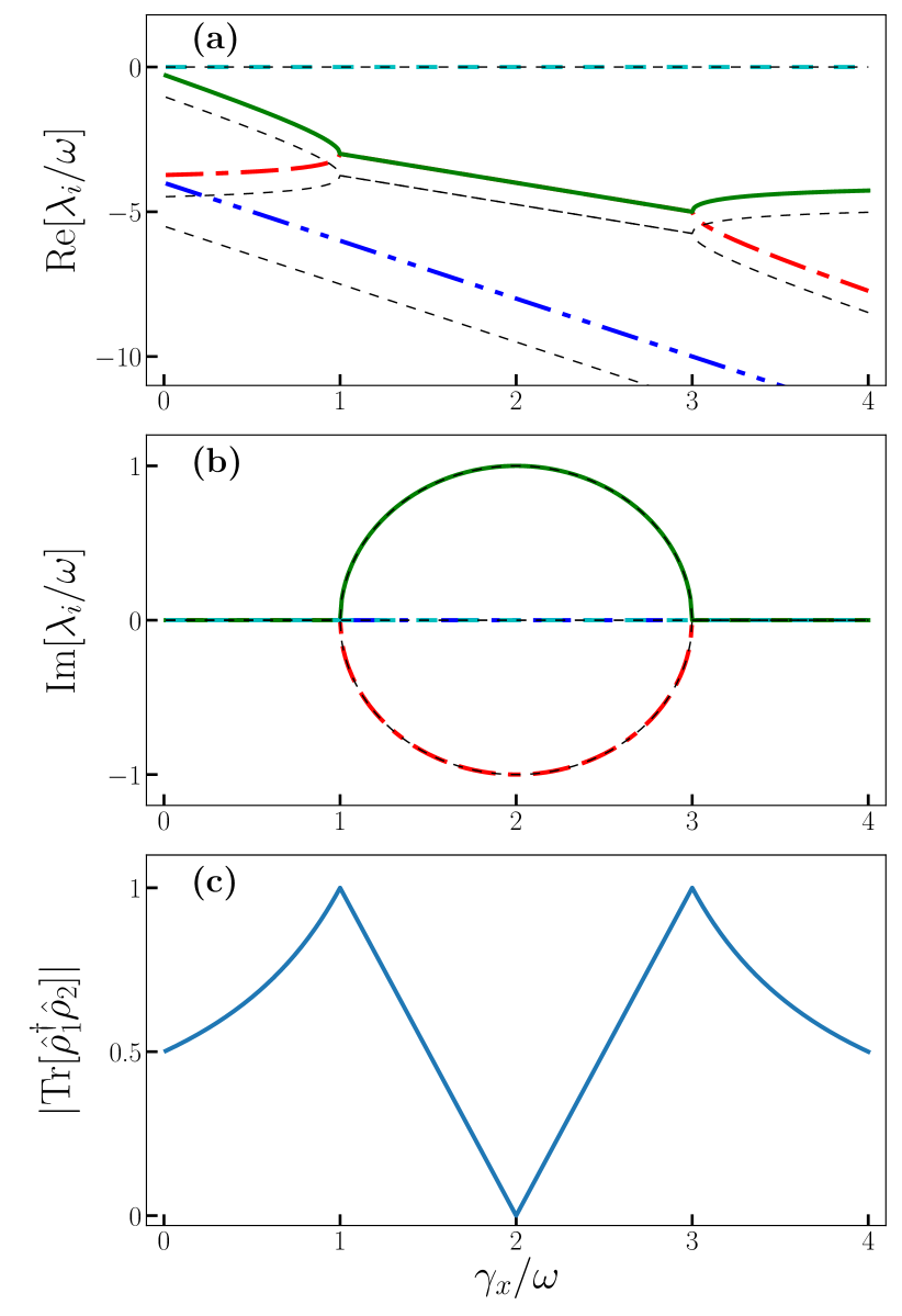
Figure 1: Spectral properties of the Liouvillian in Eq. (38) in the case of $\gamma_{y}=2\omega$. This Liouvillian has a LEP, but the associated NHH has no HEP. The thick curves represent $\gamma_{-}=0$, while the thin dashed ones are for $\gamma_{-}=\omega$. (a) Real and (b) imaginary parts of the Liouvillian eigenvalues in Eq. (40) as a function $\gamma_{x}/\omega$, i.e., the dissipation in the $\hat{\sigma}_{x}$ direction rescaled by the qubit energy $\omega$. (c) Scalar product between the two eigenmatrices $\hat{\rho}_{1}$ and $\hat{\rho}_{2}$ in Eq. (41) as a function of $\gamma_{x}/\omega$.

In this section, we address the question of whether there exists any model exhibiting LEPs but not HEPs, thus confirming Theorem 1. At first, let us consider a rather general model of a spin-$1/2$, with Hamiltonian

$$\hat{H}=\frac{\omega}{2}\hat{\sigma}_{z},$$ (37)

which evolves under the action of the three competing decay channels, ($\hat{\sigma}_{x}$, $\hat{\sigma}_{y}$, and $\hat{\sigma}_{-}$) described by

$$\mathcal{L}\hat{\rho}(t)=-i[\hat{H},\hat{\rho}(t)]+\frac{\gamma_{-}}{2}\mathcal{D}[\hat{\sigma}_{-}]\hat{\rho}(t)+\frac{\gamma_{x}}{2}\mathcal{D}[\hat{\sigma}_{x}]+\frac{\gamma_{y}}{2}\mathcal{D}[\hat{\sigma}_{y}],$$ (38)

$\hat{\sigma}_{x,\,y,\,z}$ being the Pauli matrices, $\hat{\sigma}_{\pm}=(\sigma_{x}\pm i\sigma_{y})/2$ and $\hat{\sigma}_{z}=\hat{I}-2\hat{\sigma}_{+}\hat{\sigma}_{-}$. Since this master equation is invariant under the exchange $\hat{\sigma}_{-}\to-\hat{\sigma}_{-}$, this model explicitly presents a $\mathcal{Z}_{2}$ symmetry Albert and Jiang (2014); Minganti et al. (2018). Moreover, there are several terms which can compete in determining the relaxation rate towards the steady state: (i) the Hamiltonian oscillations; (ii) the dissipation along the $x$ and $y$ axes; and (iii) the spin flips described by $\hat{\sigma}_{-}$.

First, we note that the NHH structure is trivial, since $\hat{H}_{\rm eff}$ is already diagonal in the $\hat{\sigma}_{z}$ basis, and its matrix form reads

$$\hat{H}_{\rm eff}=\frac{1}{2}\left(\begin{array}[]{cc}\omega-i\gamma_{x}-i\gamma_{y}-i\gamma_{-}&0\\ 0&-\omega-i\gamma_{x}-\gamma_{y}\\ \end{array}\right).,$$ (39)

This equation cannot present any EP, since no change in parameters can make the two eigenvalues equal.

Nevertheless, the Liouvillian can present several interesting properties. We have

$$\left\{\begin{split}\lambda_{0}&=0,\\ \lambda_{1,\,2}&=-\frac{\gamma_{-}}{2}-\gamma_{x}-\gamma_{y}\pm\Omega,\\ \lambda_{3}&=\gamma_{-}-2\left(\gamma_{y}+\gamma_{x}\right),\end{split}\right.$$ (40)

and

$$\left\{\begin{split}\hat{\rho}_{0}&\propto\rho^{SS}=\frac{1}{2\gamma_{x}+2\gamma_{y}+\gamma_{-}}\begin{pmatrix}\gamma_{x}+\gamma_{y}&0\\ 0&\gamma_{x}+\gamma_{y}+\gamma_{-}\end{pmatrix},\\ \hat{\rho}_{1,\,2}&\propto\begin{pmatrix}0&-i\omega\pm\Omega\\ \gamma_{x}-\gamma_{y}&0\\ \end{pmatrix},\\ \hat{\rho}_{3}&\propto\begin{pmatrix}-1&0\\ 0&1\\ \end{pmatrix},\end{split}\right.$$ (41)

where $\Omega=\sqrt{\gamma_{x}^{2}+\gamma_{y}^{2}-2\gamma_{x}\gamma_{y}-\omega^{2}}$.

Therefore, in the case $\gamma_{y}>\omega$, this Liouvillian exhibits two EPs, one for $\gamma_{x}=\gamma_{y}-\omega$, and one for $\gamma_{x}=\gamma_{y}+\omega$. We study this configuration for $\gamma_{-}=0$ in Fig 1. Here, the key parameter is $\Gamma$ in $\lambda_{1,\,2}$ and $\hat{\rho}_{1,\,2}$. Therefore, we can identify three regimes [cf. Figs. 1(a) and 1(b)]:

1. The case of $\gamma_{x}<\gamma_{y}-\omega$, where the dynamics is dominated by the dissipation channel $\mathcal{D}[\hat{\sigma}_{y}]$, and the decay towards the steady state is purely exponential.

2. The case of $\gamma_{y}-\omega<\gamma_{x}<\gamma_{y}+\omega$, where the competition between the dissipation along the $\hat{\sigma}_{x}$ and $\hat{\sigma}_{x}$ directions allows for Hamiltonian oscillations towards the steady state.

3. The case of $\gamma_{x}>\gamma_{y}+\omega$, when the dissipative dynamics is dominated by the damping in the $\hat{\sigma}_{x}$ direction.

This change in the spectral properties of the Liouvillian is signaled by a coalescence of the eigenvectors, as shown in Fig. 1(c). The case of $\gamma_{-}\neq 0$ is also plotted in Fig. 1 with dotted curves and shows similar spectral features, with a remarkable difference: an overall shift of $\gamma_{-}/2$ in $\lambda_{1,\,2}$, and of $\gamma_{-}$ in $\lambda_{3}$.

IV.0.1 Purely quantum exceptional points

The study of the Liouvillian in Eq. (38) naturally raises the question of the meaning of the Liouvillian EPs which are induced by quantum jumps and thus are not observed in the corresponding NHH dynamics. Indeed, the term determining the EP is $\hat{\sigma}_{x}\hat{\rho}(t)\hat{\sigma}_{x}$. According to measurement theory, this process can be interpreted as the backaction of a measurement apparatus on a system Barnett (2009). In the present case, such “reading apparatus” is the environment itself Haroche and Raimond (2006); Wiseman and Milburn (2010), which projects the system on the eigenspace of its pointer states. In this regard, this exceptional point is induced by a purely quantum effect, and is really due to the measurement and not to the “semiclassical” dissipation caused by the environment. That is, the bare presence of the measurement apparatus and the reading of it induces quantum jumps. Finally, $\hat{\rho}_{1,\,2}$ represent the loss of coherence of the density matrix into the environment. As such, these LEPs are due to this purely quantum effect, and cannot be explained by the semiclassical approximation in Eq. (39).

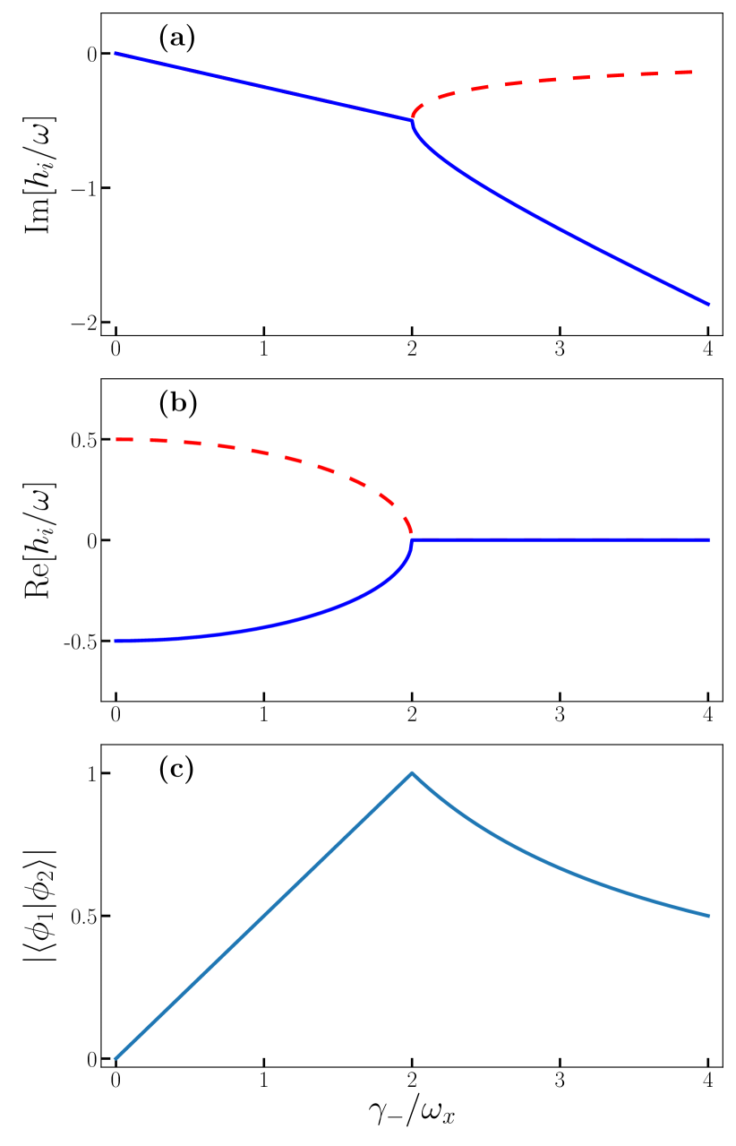
Figure 2: Spectral properties of the NHH in Eq. (44) showing an HEP. (a) Imaginary and (b) real parts of the eigenvalues in Eq. (45) as a function of $\gamma_{-}/\omega_{x}$: the ratio between the spin-flip rate and the drive. (c) Scalar product between $\ket{\phi_{1}}$ and $\ket{\phi_{2}}$, given in Eq. (46), as a function of $\gamma_{-}/\omega_{x}$.

Figure 3: Spectral properties of the Liouvillian in Eq. (43), exhibiting a LEP, but for the same parameters as the NHH studied in Fig. 2. (a) Real part and (b) imaginary parts of the Liouvillian eigenvalues in Eq. (47) as a function of $\gamma_{-}/\omega_{x}$. Note that according to Eq. (5), one should compare $\mathbb{R}\mathrm{e}\left[\lambda_{i}\right]$ with $\mathbb{I}\mathrm{m}\left[h_{i}\right]$ in Fig. 2(a), and $\mathbb{I}\mathrm{m}\left[\lambda_{i}\right]$ with $\mathbb{R}\mathrm{e}\left[h_{i}\right]$ in Fig. 2(b). (c) Scalar product between the two eigenmatrices $\hat{\rho}_{2}$ and $\hat{\rho}_{3}$, given in Eq. (48), as a function of $\gamma_{-}/\omega_{x}$.

V Example 2 of Theorem 1: a system with nonequivalent LEPs and HEPs

Here we study a model of a single dissipative driven spin exhibiting both LEPs and HEPs. This is another example obeying the condition of Theorem 1. This time, both the NHH and $\mathcal{L}$ present EPs. However, by comparing them we find several discrepancies.

This model is described by

$$\hat{H}=\frac{\omega_{x}}{2}\hat{\sigma}_{x},$$ (42)

which evolves under the action of the following Liouvillian decaying channel

$$\mathcal{L}\hat{\rho}(t)=-i[\hat{H},\hat{\rho}(t)]+\frac{\gamma_{-}}{2}\mathcal{D}[\hat{\sigma}_{-}]\hat{\rho}(t).$$ (43)

We stress that an experimental study of this system using postselection techniques has been presented in Ref. Naghiloo et al. (2019).

V.1 The non-Hermitian Hamiltonian spectrum

We begin our study by considering the following NHH

$$\hat{H}_{\rm eff}=\frac{\omega_{x}}{2}\hat{\sigma}_{x}-i\frac{\gamma_{-}}{2}\hat{\sigma}_{+}\hat{\sigma}_{-},$$ (44)

which results from Eq. (43) if we ignore the quantum jump term in $\mathcal{D}[\hat{\sigma}_{-}]$. We remark that, by the addition of a constant term $(-i\gamma_{-}\mathds{1})$, this model becomes the celebrated two-level system showing a parity-time ($\mathcal{PT}$)-symmetry breaking, extensively discussed in, e.g., Refs. El-Ganainy et al. (2018); Miri and Alù (2019). Indeed, this Hamiltonian has eigenvalues

$$h_{1,\,2}=\frac{1}{4}\left(-i\gamma_{-}\mp\zeta\right),$$ (45)

and eigenvectors

$$\ket{\phi_{1,\,2}}\propto\left[i\gamma_{-}\mp\zeta\,,\quad 2\omega_{x}\right],$$ (46)

where $\zeta=\sqrt{4\omega_{x}^{2}-\gamma_{-}^{2}}$. The imaginary and real parts of the eigenvalues $h_{i}$ are plotted in Figs. 2(a) and Figs. 2(b), respectively. Notice that panel (a) represents the imaginary part of $h_{i}$, while panel (b) focuses on the real part. In this way, one can directly compare the results for $\mathbb{I}\mathrm{m}\left[h_{i}\right]$ with those $\mathbb{R}\mathrm{e}\left[\lambda_{i}\right]$ in Figs. 2(a) and 3(a), taking into account the $(-i)$ factor in Eq. (5).

For $\gamma_{-}/\omega_{x}=2$, the eigenvalues of $\hat{H}_{\rm eff}$ are degenerate, $h_{1}=h_{2}$, and the corresponding eigenvectors $\ket{\phi_{1}}$ and $\ket{\phi_{2}}$ of $\hat{H}_{\rm eff}$ coalesce (see also Fig. 2). Since this model exhibits some “semiclassical” EPs, the natural question arises, what happens to these EPs once the quantum jump term is taken into account? Since $[\hat{\sigma}_{-},\hat{\sigma}_{x}]\neq 0$ and $\hat{\sigma}_{-}\ket{\phi_{1,\,2}}\neq 0$, we expect that the spectral structure of these two models can be remarkably different (cf. Lemma 4 and Theorem 1).

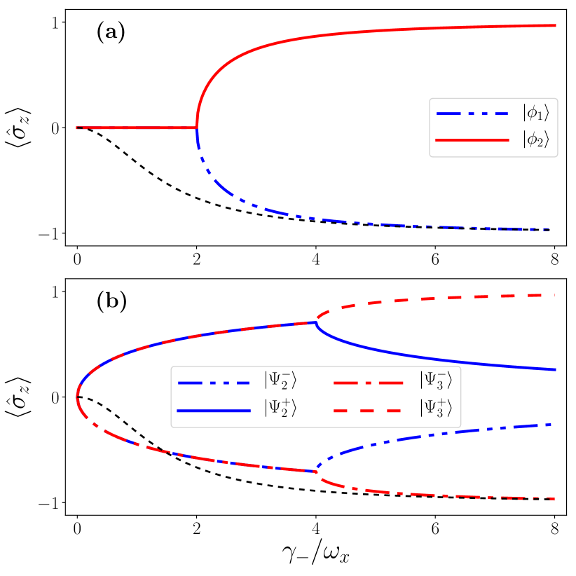
Figure 4: Expectation value of $\braket{\hat{\sigma}_{z}}$ as a function of $\gamma_{-}/\omega_{x}$. In both panels the dashed black curves represent the mean value of photons in the steady state. (a) NHH eigenvectors [Eq. (46)]. (b) Eigenvectors obtained via the spectral decomposition of $\hat{\rho}_{3,\,4}$ [cf. Eq. (50)].

V.2 The Liouvillian spectrum

We now consider the complete master equation in Eq. (43). The Liouvillian eigenvalues are

$$\begin{split}\lambda_{0}&=0,\\ \lambda_{1}&=-\frac{\gamma_{-}}{2},\\ \lambda_{2,\,3}&=-\frac{3}{4}\gamma_{-}\pm\eta/4,\\ \end{split}$$ (47)

while the eigenmatrices are

$$\begin{split}\hat{\rho}_{0}&\propto\hat{\rho}_{\rm ss}=\frac{1}{\gamma_{-}^{2}+2\omega_{x}^{2}}\begin{pmatrix}\gamma_{-}^{2}+\omega_{x}^{2}&i\gamma_{-}\omega_{x}\\ -i\gamma_{-}\omega_{x}&\omega_{x}^{2}\end{pmatrix},\\ \hat{\rho}_{1}&\propto\begin{pmatrix}0&1\\ 1&0\\ \end{pmatrix},\\ \hat{\rho}_{2,\,3}&\propto\begin{pmatrix}-\gamma_{-}\pm\eta&4i\omega_{x}\\ -4i\omega_{x}&\gamma_{-}\mp\eta\end{pmatrix},\end{split}$$ (48)

where $\eta=\sqrt{\gamma_{-}^{2}-16\omega_{x}^{2}}$. Hence, we expect a LEP for $\gamma_{-}=4\omega_{x}$.

In Figs. 3(a) and 3(b) we plot the real and imaginary parts of the eigenvalues $\lambda_{i}$ obtained in Eq. (47). Indeed, we note that, for $\gamma_{-}=4\omega_{x}$, $\lambda_{2,\,3}$ coalesce. As expected, this EP is signaled by the coalescence of the two associated right eigenmatrices [Fig. 3(c) and Eq. (48)]. We note that the decay along the $\hat{\sigma}_{x}$ channel is dominated by $\lambda_{1}$ and therefore to see interesting phenomena one should study either $\hat{\sigma}_{y}$ or $\hat{\sigma}_{z}$.

V.3 Comparison of HEPs and LEPs

The question naturally arises: what is the link between the NHH EPs and Liouvillian EPs? To answer this question we analyze the spectra of $\hat{\rho}_{2}$ and $\hat{\rho}_{3}$ using the spectral decomposition introduced in Sec. III.4. We obtain

$$\begin{split}\hat{\rho}_{2,\,3}\propto\ket{\Psi_{2,\,3}^{+}}\bra{\Psi_{2,\,3}^{+}}-\ket{\Psi_{2,\,3}^{-}}\bra{\Psi_{2,\,3}^{-}},\end{split}$$ (49)

where

$$\begin{split}\ket{\Psi_{2}^{\pm}}&\propto\left[i\left(-\gamma_{-}+\eta\pm\sqrt{2\gamma_{-}\left(\gamma_{-}-\eta\right)}\right),\quad 4\omega_{x}\right],\\ \ket{\Psi_{3}^{\pm}}&\propto\left[-i\left(\gamma_{-}+\eta\pm\sqrt{2\gamma_{-}\left(\gamma_{-}+\eta\right)}\right),\quad 4\omega_{x}\right].\end{split}$$ (50)

By comparing these with $\ket{\phi_{1}}$ and $\ket{\phi_{1}}$ in Eq. (46), we note that their structures present several similarities when substituting $\omega_{x}\to 2\omega_{x}$. To better capture similarity between the LEPs and HEPs, in Fig. (4) we plot the expectation value $\braket{\hat{\sigma}_{z}}$ taken over the states $\ket{\Psi_{1,\,2}}$ [panel (a)] and $\ket{\Psi_{3,\,4}^{\pm}}$ [panel (b)]. We observe that, surprisingly, the NHH captures the behavior of $\hat{\rho}_{3}$, but not of $\hat{\rho}_{2}$, even if $|\mathbb{R}\mathrm{e}\left[\lambda_{3}\right]|<|\mathbb{R}\mathrm{e}\left[\lambda_{4}\right]|$. Finally, we remark that the addition of the quantum jumps produces a double bifurcation, and thus we conclude that the NHH approximation is not able to capture the dynamics of $\hat{\sigma}_{x,y}$ towards the steady state.

Therefore, we may argue that the effect of quantum jumps in this model is twofold: On the one hand, as a consequence of Theorem 1, quantum jumps modify the structure of the eigenstates of the NHH. On the other hand, $\{\ket{\Psi_{2}^{\pm}},\,\ket{\Psi_{3}^{\pm}}\}$ maintain some similarities to $\{\ket{\phi_{1}},\,\ket{\phi_{2}}\}$. In this regard, in the next section we will see that when this two-level system is the effective description of a bigger bosonic system in a semiclassical limit, the effect of quantum jumps will be to introduce a mixing of the “eigenstates” of the corresponding NHH, according to Theorem 2.

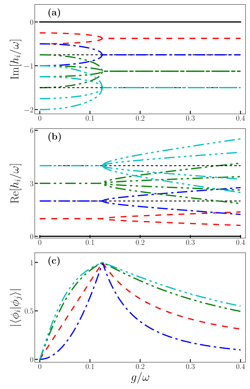
Figure 5: Spectral properties of the NHH in Eq. (53). (a) Imaginary and (b) real parts of the eigenvalues as a function of $g/\omega$, i.e., the coupling between the cavities rescaled by the frequency of each cavity. (c) Scalar product between the eigenvectors associated with the EPs, as a function of $g/\omega$. Here, the parameters used are $\gamma_{a}=\omega$, $\gamma_{b}=\omega/2$.

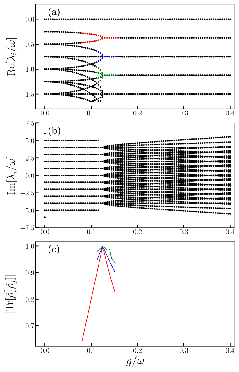
Figure 6: (Colors online) Spectral properties of the full Liouvillian in Eq. (52). (a) Real and (b) imaginary parts of the eigenvalues as a function of $g/\omega$. Note that according to Eq. (5), one should compare $\mathbb{R}\mathrm{e}\left[\lambda_{i}\right]$ with $\mathbb{I}\mathrm{m}\left[h_{i}\right]$ in Fig. 5(a), $\mathbb{I}\mathrm{m}\left[\lambda_{i}\right]$ with $\mathbb{R}\mathrm{e}\left[h_{i}\right]$ in Fig. 5(b). (c) Scalar product between the eigenvectors associated with the EP as a function of $g/\omega$. We were not able to extract this quantity for all the values of $g/\omega$ due to numerical problems in correctly sorting the eigenvectors. Indeed, the eigenmatrices of $\mathcal{L}$ no longer obey the total-excitation conservation law valid for the NHH. Here the parameters used are $\gamma_{a}=\omega$, $\gamma_{b}=\omega/2$.

VI Example of theorem 2:
A semiclassical model with equivalent HEPs and LEPs

The two previous examples proved that in the “fully quantum” limit, the NHH fails to completely capture the underlying physics. In this section, we consider, instead, a model whose semiclassical limit correctly predicts the features of the EPs as an example of Theorem 2.

Let us consider two coupled bosonic modes, characterized by

$$\hat{H}=\omega\left(\hat{a}^{\dagger}\hat{a}+\hat{b}^{\dagger}\hat{b}\right)+g\left(\hat{a}^{\dagger}\hat{b}+\hat{b}^{\dagger}\hat{a}\right).$$ (51)

and

$$\mathcal{L}=-i[\hat{H},\mathchoice{\mathbin{\vbox{\hbox{\scalebox{0.5}{$\displaystyle\bullet$}}}}}{\mathbin{\vbox{\hbox{\scalebox{0.5}{$\textstyle\bullet$}}}}}{\mathbin{\vbox{\hbox{\scalebox{0.5}{$\scriptstyle\bullet$}}}}}{\mathbin{\vbox{\hbox{\scalebox{0.5}{$\scriptscriptstyle\bullet$}}}}}]+\frac{\gamma_{a}}{2}\mathcal{D}[\hat{a}]+\frac{\gamma_{b}}{2}\mathcal{D}[\hat{b}].$$ (52)

The key element in this model is the imbalance of the dissipation rates $\gamma_{a}\neq\gamma_{b}$, resulting in one of the two modes to be dissipated more quickly than the other.

Physically, this model can be interpreted as photons hopping between two cavities, one of which has a smaller quality factor than the other. For small coupling $g$, this dissipation imbalance tends to localize bosons in the less dissipative cavity before eventually the system loses all the particles to the environment. For large coupling $g$, the two modes are hybridized, and the localization effect of dissipation cannot take place anymore. The transition from local-to-nonlocal long-time dynamics can be signaled by the presence of an EP.

As already shown in Ref. Glauber (1966), the dynamics of these two linearly coupled quantum oscillators is (nearly) classical in nature. Note that this prototype model of a linear coupler is mathematically equivalent to the models of a parametric frequency converter and a beam splitter. These models are of fundamental importance in quantum optics. In the dissipation-free case, various two-mode phase-space quasiprobability distributions (like the Husimi, Wigner, and Glauber-Sudarshan functions) remain constant along purely semiclassical trajectories. Within this model, an initially semiclassical state remains semiclassical during its evolution. In a dissipation-free model, the degree of nonclassicality (or classicality) of an initially quantum state remains unchanged. This property has been used to define an operational measure of nonclassicality Asbóth et al. (2005); Miranowicz et al. (2015a, b). So, it is convenient for us to use this model to compare the two types of EPs in the semiclassical limit.

VI.1 Hamiltonian EPs

The NHH associated with Eq. (52) reads

$$\hat{H}_{\rm eff}=\left(\omega-i\frac{\gamma_{a}}{2}\right)\hat{a}^{\dagger}\hat{a}+\left(\omega-i\frac{\gamma_{b}}{2}\right)\hat{b}^{\dagger}\hat{b}+g\left(\hat{a}^{\dagger}\hat{b}+\hat{b}^{\dagger}\hat{a}\right).$$ (53)

This matrix couples subspaces with a constant number of particles, resulting in a block-diagonal NHH.

In Figs. 5(a) and 5(b) we plot the imaginary and real part of the eigenvalues $h_{i}$ of $\hat{H}_{\rm eff}$, proving that the system admits a set of EPs, each one characterized by a different number of excitations [cf. panel (c), where the scalar product of the eigenvectors associated with the EPs become 1]. Most importantly, the system exhibits all the EPs for the same value of $g/\omega$.

VI.2 Liouvillian EPs

We perform the same spectral analysis on the Liouvillian in Eq. (52) in Fig. 6. Similarly to Fig. 5, we observe a ladder of EPs, characterized by really similar spectral features. We notice that, however, in accordance to Theorem 1, no EPs occur in the steady state, even if the NHH correctly captures the parameter $g/\omega$ for which the system has an EP. Moreover, we notice in panel (b) that many eigenvectors have an EP with imaginary part zero, in contrast to Fig. 5(a). Finally, in panel (c) we demonstrate that the appropriate eigenmatrices, i.e., those coalescing at the EP, have a scalar product equal to 1 for $g=0.125\omega$, proving that indeed the bifurcation is produced by an EP.

VI.3 Comparison of HEPs and LEPs

Let us begin our discussion by considering the time evolution of the expectation value of $\braket{\hat{a}}$ and $\braket{\hat{b}}$. For the NHH, we have $\partial_{t}\braket{\hat{a}}=-i\braket{\left[\hat{a},\hat{H}_{\rm eff}\right]}$, while for the Liouvillian,

$$\partial_{t}\braket{\hat{a}}=-i\braket{\left[\hat{a},\hat{H}\right]}+\frac{\gamma}{2}\mathrm{Tr}\!\left[\hat{a}\mathcal{D}[\hat{a}\hat{\rho}(t)\right].$$ (54)

Remarkably, both equations lead to the same result,

$$\partial_{t}\begin{bmatrix}\braket{\hat{a}}\\ \braket{\hat{b}}\end{bmatrix}=-i\begin{pmatrix}\omega-i\frac{\gamma_{a}}{2}&g\\ g&\omega-i\frac{\gamma_{b}}{2}\end{pmatrix}\begin{bmatrix}\braket{\hat{a}}\\ \braket{\hat{b}}\end{bmatrix}.$$ (55)

The previous equation confirms that the some of the HEP and LEP must be similar (i.e., same eigenvalues and eigenvectors) in order to reproduce the same dynamics of these expectation values. However, this does not mean that the whole spectral structure is identical.

As for the similarity, we note that Theorem 2 can be applied. Indeed, let us consider the subspace with no excitation, where $\hat{H}_{\rm eff}\ket{0,0}=0\ket{0,0}$. It follows that ${\ket{\phi_{0}}=\ket{0,0}}$, since $\hat{a}\ket{0,0}=\hat{b}\ket{0,0}=0$.

We can easily verify the validity of Theorem 2 by considering $\hat{H}_{\rm eff}$ in the subspace with one excitation (i.e., $\ket{1,0}$ and $\ket{0,1}$), where

$$\hat{H}_{\rm eff}=\left(\omega-\frac{i\bar{\gamma}}{2}\right)\mathds{1}+\begin{pmatrix}-i\frac{\gamma}{2}&g\\ g&i\frac{\gamma}{2}\end{pmatrix},$$ (56)

for $\bar{\gamma}=(\gamma_{a}+\gamma_{b})/2$, and $\gamma=(\gamma_{a}-\gamma_{b})/2$. The eigenvalues are

$$h_{i}=\omega-\frac{i\bar{\gamma}}{2}\pm\theta,$$ (57)

and the eigenfunctions of $\hat{H}_{\rm eff}$ are

$$\ket{\phi_{1,2}}=\left(-i\frac{\gamma}{2}\pm\theta\right)\ket{0,1}+g\ket{1,0},$$ (58)

where $\theta^{2}=g^{2}-\gamma^{2}/4$. We remark that this equation is identical to Eq. (44) by the addition of a constant term $(-i\gamma_{-}\mathds{1})$. Clearly, the model exhibits an EP for $g=\gamma/2$, where $\ket{\phi_{1}}$ and $\ket{\phi_{2}}$ coalesce.

If we consider now $\hat{\rho}_{1}=\ket{\phi_{1,2}}\bra{0,0}$, since we have $\mathcal{D}[\hat{a}]\hat{\rho}_{1}=\mathcal{D}[\hat{b}]\hat{\rho}_{1}=0$, then

$$\mathcal{L}\hat{\rho}_{1}=-i\left(\hat{H}_{\rm eff}\hat{\rho}_{1}-\hat{\rho}_{1}\hat{H}_{\rm eff}^{\dagger}\right)=-ih_{i}\ket{\phi_{1,2}}\bra{0,0}.$$ (59)

We have numerically confirmed this behavior for the whole spectrum of the Liouvillian and the NHH up to a cutoff of nine excitations per site.

Finally, to correctly interpret $\hat{\rho}_{1}$, we consider the eigendecomposition of $\hat{\rho}_{1}+\hat{\rho}_{2}$ (which, by construction, is Hermitian), obtaining $\hat{\rho}_{1}+\hat{\rho}_{2}=\ket{\Psi_{1}}\bra{\Psi_{1}}-\ket{\Psi_{2}}\bra{\Psi_{2}}$, where

$$\begin{split}\ket{\Psi_{1,\,2}}&=\frac{\ket{0,0}}{\sqrt{2}}\pm\frac{(-1+i)\ket{0,1}+(1+i)\ket{1,0}}{2\sqrt{2}}.\\ \end{split}$$ (60)

All the other eigenstates $\hat{\rho}_{i}$ which are not of the form $\ket{0,0}\bra{\phi_{l}}$ or $\ket{\phi_{l}}\bra{0,0}$, instead, have different characteristics and cannot be easily recast in terms of simple combinations of $\ket{\phi_{l}}\bra{\phi_{m}}$.

Again, we have confirmed the results of Theorem 1 in an example satisfying Theorem 2, showing that, indeed, even if the EP position and some of the LEPs can be captured by the NHH, that is not the case for all the eigenvectors.

VII Conclusions and discussion

In this paper, we addressed the question of how to define EPs in the fully quantum regime, i.e., by including quantum jumps. Standard EPs (i.e., HEPs) correspond to the spectra of NHHs, and thus quantum jumps do not have any effect on these. Of course, HEPs can be formally applied also for system far from the semiclassical limit, but the question arises whether they properly grasp the quantum nature of nonconservative systems.

Our proposal of defining EPs for the quantum regime is based on analyzing the eigenfrequency and eigenstate degeneracies of the spectra of Liouvillians. Thus, these EPs are referred to as Liouvillian EPs or LEPs.

Our approach was motivated by the standard Lindblad master equation and its quantum trajectory interpretation, which includes both the continuous and the nonunitary dissipation terms, $\hat{\Gamma}_{\mu}^{\dagger}\hat{\Gamma}_{\mu}\hat{\rho}(t)+\hat{\rho}(t)\hat{\Gamma}_{\mu}^{\dagger}\hat{\Gamma}_{\mu}$, and the quantum jump terms, $\hat{\Gamma}_{\mu}\hat{\rho}(t)\hat{\Gamma}_{\mu}^{\dagger}$. We note that the calculation of an EP based on NHHs includes the same continuous nonunitary dissipation term but not the quantum jump term.

The core results of this paper concern the comparison of Liouvillian and Hamiltonian EPs. We proved two main theorems: Theorem 1 showing that LEPs and HEPs have essentially different properties in the quantum regime, and Theorem 2 specifying some conditions under which LEPs and HEPs exhibit the same properties in the semiclassical limit. We compared explicitly LEPs and HEPs for some quantum and semiclassical prototype models:

1. A dissipative two-level system presenting LEPs but no HEPs, i.e., a quantum model without a semiclassical analog;

2. A dissipative two-level system presenting differences between LEPs and HEPs;

3. Two linearly coupled dissipative quantum oscillators (a linear coupler or a parametric frequency converter), which have semiclassical dynamics Glauber (1966).

We showed that, in general, LEPs and HEPs can have essentially different properties (examples 1 and 2). Moreover, the model of example 3 enabled us to show explicitly that LEPs and HEPs become essentially equivalent in the semiclassical limit.

Note that we were not discussing here any applications of EPs. Further research is required to generalize various semiclassical predictions of novel photonic functionalities (mentioned in, e.g., reviews Özdemir et al. (2019); Miri and Alù (2019)) to the quantum regime. These applications might include an enhanced control of physical processes (e.g., scattering and transmission) at EPs in composite systems with loss, gain, and gain saturation. For example, in a recent study of Arkhipov et al. (2019b), the Scully-Lamb laser model in its semiclassical limit was applied to describe the experimentally observed light nonreciprocity and HEPs reported in Peng et al. (2014b); Chang et al. (2014) for parity-time-symmetric whispering-gallery microcavities. The application of the formalism developed in this paper could enable to study LEPs in the Scully-Lamb laser model, assuming weak gain saturation, in its full quantum regime Arkhipov et al. (2019a).

Another important application of EPs could be a possible enhancement of the sensitivity of the energy splitting and frequency detection at HEPs, as discussed theoretically in, e.g., Refs. Wiersig (2014); Zhang et al. (2015); Wiersig (2016); Ren et al. (2017); Kuo et al. and observed experimentally in Refs. Chen et al. (2017); Hodaei et al. (2017); Chen et al. (2018); Liu et al. (2016). Indeed, even a very small perturbation applied to an NHH system at an EP can lift the system eigenfrequency degeneracy, leading to a detectable energy splitting. However, more detailed analyses of noise showed some fundamental limits of HEP-enhanced sensors Langbein (2018); Lau and Clerk (2018); Mortensen et al. (2018); Wolff et al. (2019); Zhang et al. ; Chen et al. (2019). In particular, a recent study Langbein (2018) indicates that enhanced sensitivity does not necessarily imply enhanced precision of sensors operating at EPs. Moreover, the importance of the unraveling protocol to obtain an enhancement of the measure sensitivity around an EP was proved in Ref. Lau and Clerk (2018). In particular, for the nonreciprocal system of Ref. Lau and Clerk (2018), homodyne (heterodyne) detection was found to have the largest enhancement. In this regard, our extension to the full quantum limit allows an easy discussion of such protocols. Further work (which, however, is beyond the scope of this paper) is required to clarify the quantum-noise-limited performance not only of generalized LEP-based sensors, but even of standard HEP-based sensors.

LEPs can signal a second-order phase transition of driven dissipative systems, as pointed out in Minganti et al. (2018). In this regard, the quest for enhanced sensitivity exploiting EPs can be corroborated by the diverging susceptibility characterizing symmetry breaking. Extensive analyses of second-order phase transitions have been carried out for several types of open systems, ranging from optical cavities Bartolo et al. (2016); Biella et al. (2017); Savona (2017); Overbeck et al. (2017); Rota et al. (2019), to spin models Lee et al. (2011); Kessler et al. (2012); Lee et al. (2013); Jin et al. (2016); Rota et al. (2017, 2018), and optomechanical systems Benito et al. (2016); Sánchez Muñoz et al. (2018). Moreover, EPs are relevant for the classification of topological phases of matter Leykam et al. (2017); González and Molina (2017); Hu et al. (2017); Gao et al. (2018); Zhou et al. (2018); Liu et al. (2019); Bliokh et al. (2019); van Caspel et al. (2019); Ge et al.

We stress that the proposed concept of LEPs can be applied to quantum system dynamics both with and without quantum jumps, while the standard concept of HEPs is limited to describing the dynamics of a system without quantum jumps. This is because HEPs are (degenerate) eigenvalues of operators (i.e., non-Hermitian Hamiltonians) rather than of superoperators (e.g., Liouvillians). Thus, in the semiclassical and classical regimes where quantum jumps do not change the dynamics, the concept of LEPs is a complete alternative to the concept of HEPs. Otherwise (i.e., when quantum jumps cannot be ignored), the approach based on HEPs fails and should be replaced by that of, e.g., LEPs. Moreover, the use of the Liouvillian is crucial to correctly identify and characterize LEPs without an NHH counterpart. This formalism has the advantage to capture both EPs resulting from the NHH and the quantum jumps, which otherwise could not be described in the same manner.

The analysis of EPs in the quantum regime is thus a timely subject. These phenomena could be fully tractable in state-of-the-art experimental platforms, such as circuit quantum-electrodynamics (QED) setups. In these systems, the precise control of amplification, dissipation, and coupling strength in principle allows EPs to be attained and characterized in the full quantum regime Naghiloo et al. (2019); Gu et al. (2017).

Appendix A Basic properties of superoperators

Here, for pedagogical reasons and following the discussion in Minganti (2018), we recall useful properties of superoperators, i.e., linear operators acting on the vector space of operators. That is (as stated in Carmichael (2007)), “superoperators act on operators to produce new operators, just as operators act on vectors to produce new vectors.”

An example of such a superoperator is the commutator $\mathcal{A}=\left[\hat{A},\mathchoice{\mathbin{\vbox{\hbox{\scalebox{0.5}{$\displaystyle\bullet$}}}}}{\mathbin{\vbox{\hbox{\scalebox{0.5}{$\textstyle\bullet$}}}}}{\mathbin{\vbox{\hbox{\scalebox{0.5}{$\scriptstyle\bullet$}}}}}{\mathbin{\vbox{\hbox{\scalebox{0.5}{$\scriptscriptstyle\bullet$}}}}}\right]=\hat{A}\mathchoice{\mathbin{\vbox{\hbox{\scalebox{0.5}{$\displaystyle\bullet$}}}}}{\mathbin{\vbox{\hbox{\scalebox{0.5}{$\textstyle\bullet$}}}}}{\mathbin{\vbox{\hbox{\scalebox{0.5}{$\scriptstyle\bullet$}}}}}{\mathbin{\vbox{\hbox{\scalebox{0.5}{$\scriptscriptstyle\bullet$}}}}}-\mathchoice{\mathbin{\vbox{\hbox{\scalebox{0.5}{$\displaystyle\bullet$}}}}}{\mathbin{\vbox{\hbox{\scalebox{0.5}{$\textstyle\bullet$}}}}}{\mathbin{\vbox{\hbox{\scalebox{0.5}{$\scriptstyle\bullet$}}}}}{\mathbin{\vbox{\hbox{\scalebox{0.5}{$\scriptscriptstyle\bullet$}}}}}\hat{A}$. With this notation, we mean that $\mathcal{A}$ acting on $\hat{\rho}$ is such that $\mathcal{A}\hat{\rho}=\hat{A}\hat{\rho}-\hat{\rho}\hat{A}$, and the dot simply indicates where the argument of the superoperator is to be placed. Moreover, we adopt the convention that the action is always on the operator the closest to the right-hand side of the dot. Superoperators can also “embrace” their operators, e.g., $\mathcal{A}=\hat{A}\mathchoice{\mathbin{\vbox{\hbox{\scalebox{0.5}{$\displaystyle\bullet$}}}}}{\mathbin{\vbox{\hbox{\scalebox{0.5}{$\textstyle\bullet$}}}}}{\mathbin{\vbox{\hbox{\scalebox{0.5}{$\scriptstyle\bullet$}}}}}{\mathbin{\vbox{\hbox{\scalebox{0.5}{$\scriptscriptstyle\bullet$}}}}}\hat{B}$ is such that $\mathcal{A}\hat{\rho}=\hat{A}\hat{\rho}\hat{B}$. More generally, all superoperators can be represented as product of the right-hand action superoperator $R[\hat{O}]\,\mathchoice{\mathbin{\vbox{\hbox{\scalebox{0.5}{$\displaystyle\bullet$}}}}}{\mathbin{\vbox{\hbox{\scalebox{0.5}{$\textstyle\bullet$}}}}}{\mathbin{\vbox{\hbox{\scalebox{0.5}{$\scriptstyle\bullet$}}}}}{\mathbin{\vbox{\hbox{\scalebox{0.5}{$\scriptscriptstyle\bullet$}}}}}=\mathchoice{\mathbin{\vbox{\hbox{\scalebox{0.5}{$\displaystyle\bullet$}}}}}{\mathbin{\vbox{\hbox{\scalebox{0.5}{$\textstyle\bullet$}}}}}{\mathbin{\vbox{\hbox{\scalebox{0.5}{$\scriptstyle\bullet$}}}}}{\mathbin{\vbox{\hbox{\scalebox{0.5}{$\scriptscriptstyle\bullet$}}}}}\,\hat{O}$ and of the left-hand action superoperator $L[\hat{O}]\,\mathchoice{\mathbin{\vbox{\hbox{\scalebox{0.5}{$\displaystyle\bullet$}}}}}{\mathbin{\vbox{\hbox{\scalebox{0.5}{$\textstyle\bullet$}}}}}{\mathbin{\vbox{\hbox{\scalebox{0.5}{$\scriptstyle\bullet$}}}}}{\mathbin{\vbox{\hbox{\scalebox{0.5}{$\scriptscriptstyle\bullet$}}}}}=\hat{O}\,\mathchoice{\mathbin{\vbox{\hbox{\scalebox{0.5}{$\displaystyle\bullet$}}}}}{\mathbin{\vbox{\hbox{\scalebox{0.5}{$\textstyle\bullet$}}}}}{\mathbin{\vbox{\hbox{\scalebox{0.5}{$\scriptstyle\bullet$}}}}}{\mathbin{\vbox{\hbox{\scalebox{0.5}{$\scriptscriptstyle\bullet$}}}}}$.

A.1 Vectorization and matrix representation of superoperators

Since the operators form a vector space, it is possible to provide a vectorized representation $\vec{A}$ of each element $\hat{A}$ in $H\otimes H$. For example,

$$\hat{A}=\begin{pmatrix}a&b\\ c&d\end{pmatrix}\longrightarrow\vec{A}=\begin{pmatrix}a\\ b\\ c\\ d\end{pmatrix}.$$ (61)

Consequently, to any linear superoperator $\mathcal{A}$ it is possible to associate its matrix representation $\bar{\bar{\mathcal{A}}}$.

More generally, given an orthonormal basis of the Hilbert space $\{\ket{n}\}$, for a generic operator $\hat{\xi}$ we have

$$\begin{split}\hat{\xi}=\sum_{m,n}c_{m,n}\ket{m}\bra{n}\longrightarrow\vec{\xi}&=\sum_{m,n}c_{m,n}\ket{m}\otimes\bra{n}^{\rm TR}\\ &=\sum_{m,n}c_{m,n}\ket{m}\otimes\ket{n^{*}},\end{split}$$ (62)

where $\rm TR$ represents the transpose, while $*$ is the complex conjugate. To obtain the matrix form of any superoperator, we must describe the right- and left-hand action superoperators $R[\hat{O}]$ and $L[\hat{O}]$ as matrices $\bar{\bar{R}}[\hat{O}]$ and $\bar{\bar{L}}[\hat{O}]$. One has

$$\begin{split}\bar{\bar{R}}[\hat{O}]\vec{\xi}&=\bar{\bar{R}}[\hat{O}]\sum_{m,n}c_{m,n}\ket{m}\otimes\ket{n^{*}}=\overrightarrow{\hat{\xi}\hat{O}}\\ &=\sum_{m,n}c_{m,n}\,\ket{m}\otimes(\bra{n}\hat{O})^{\rm TR}\\ &=\sum_{m,n}c_{m,n}\,\ket{m}\otimes(\hat{O}^{\rm TR}\ket{n^{*}})=(\mathds{1}\otimes\hat{O}^{\rm TR})\vec{\xi}.\end{split}$$ (63)

Analogously, we have

$$\bar{\bar{L}}[\hat{O}]\vec{\xi}=(\hat{O}\otimes\mathds{1})\vec{\xi}.$$ (64)

From the result of Eqs. (63) and (64), we can eventually write any Liouvillian $\mathcal{L}=-i\left[\hat{H},\mathchoice{\mathbin{\vbox{\hbox{\scalebox{0.5}{$\displaystyle\bullet$}}}}}{\mathbin{\vbox{\hbox{\scalebox{0.5}{$\textstyle\bullet$}}}}}{\mathbin{\vbox{\hbox{\scalebox{0.5}{$\scriptstyle\bullet$}}}}}{\mathbin{\vbox{\hbox{\scalebox{0.5}{$\scriptscriptstyle\bullet$}}}}}\right]+\mathcal{D}[\hat{\Gamma}]$ (for simplicity, here, with only one jump operator $\hat{\Gamma}$) in the form

$$\begin{split}\bar{\bar{\mathcal{L}}}&=-i\left[\bar{\bar{L}}(\hat{H})-\bar{\bar{R}}(\hat{H})\right]+\bar{\bar{L}}(\hat{\Gamma})\bar{\bar{R}}(\hat{\Gamma}^{\dagger})-\frac{\bar{\bar{L}}(\hat{\Gamma}^{\dagger}\hat{\Gamma})}{2}-\frac{\bar{\bar{R}}(\hat{\Gamma}^{\dagger}\hat{\Gamma})}{2}\\ &=-i\left(\hat{H}\otimes\mathds{1}-\mathds{1}\otimes\hat{H}^{\rm TR}\right)+\hat{\Gamma}\otimes\hat{\Gamma}^{*}-\frac{\hat{\Gamma}^{\dagger}\hat{\Gamma}\otimes\mathds{1}}{2}-\frac{\mathds{1}\otimes\hat{\Gamma}^{\rm TR}\hat{\Gamma}^{*}}{2}.\end{split}$$ (65)

Similarly, we obtain the Liouvillian without quantum jumps $\mathcal{L}^{\prime}$ and its matrix representation

$$\bar{\bar{\mathcal{L}^{\prime}}}=-i\left(\hat{H}\otimes\mathds{1}-\mathds{1}\otimes\hat{H}^{\rm TR}\right)-\frac{\hat{\Gamma}^{\dagger}\hat{\Gamma}\otimes\mathds{1}+\mathds{1}\otimes\hat{\Gamma}^{\rm TR}\hat{\Gamma}^{*}}{2},$$ (66)

while the quantum jump term reads $\mathcal{J}[\hat{\Gamma}]=\hat{\Gamma}\otimes\hat{\Gamma}^{*}$.

This procedure can be easily generalized to multiple quantum jump operators.

A.2 Hilbert-Schmidt inner product and Hermitian conjugation

In order to discuss the coalescence of eigenstates at an EP, it is useful to introduce a scalar product. Since there is no intrinsic definition of an inner product in the operator space $H\otimes H$, we introduce the Hilbert-Schmidt product:

$$\langle\hat{A}|\hat{B}\rangle=\mathrm{Tr}\!\left[\hat{A}^{\dagger}\hat{B}\right].$$ (67)

Hence, the norm of an operator is

$$\|\hat{A}\|^{2}=\mathrm{Tr}\!\left[\hat{A}^{\dagger}\hat{A}\right].$$ (68)

That is, given two matrices

$$\hat{A}=\begin{pmatrix}a&b\\ c&d\end{pmatrix},\quad\hat{E}=\begin{pmatrix}e&f\\ g&h\end{pmatrix},$$ (69)

one has

$$\begin{split}\braket{\hat{A}}{\hat{E}}&=\begin{pmatrix}a^{*}&b^{*}&c^{*}&d^{*}\end{pmatrix}\begin{pmatrix}e&f&g&h\end{pmatrix}^{\rm TR}\\ &=a^{*}e+b^{*}f+c^{*}g+d^{*}h=\mathrm{Tr}\!\left[\hat{A}^{\dagger}\hat{E}\right].\end{split}$$ (70)

Most importantly, having introduced the inner product for the operators, it is possible to introduce the Hermitian adjoint of $\mathcal{A}$, which by definition is $\mathcal{A}^{\dagger}$ such that:

$$\braket{\hat{\xi}}{\mathcal{A}\hat{\chi}}=\braket{\mathcal{A}^{\dagger}\hat{\xi}}{\hat{\chi}}.$$ (71)

The rules to obtain such an adjoin, however, are not the same as in the case of operators. Consider the most general linear superoperator $\mathcal{A}=\hat{A}\mathchoice{\mathbin{\vbox{\hbox{\scalebox{0.5}{$\displaystyle\bullet$}}}}}{\mathbin{\vbox{\hbox{\scalebox{0.5}{$\textstyle\bullet$}}}}}{\mathbin{\vbox{\hbox{\scalebox{0.5}{$\scriptstyle\bullet$}}}}}{\mathbin{\vbox{\hbox{\scalebox{0.5}{$\scriptscriptstyle\bullet$}}}}}\hat{B}$. Exploiting the definition of the Hermitian adjoin we have

$$\begin{split}\braket{\hat{\xi}}{\mathcal{A}\hat{\chi}}&=\mathrm{Tr}\!\left[\xi^{\dagger}\hat{A}\hat{\chi}\hat{B}\right]=\mathrm{Tr}\!\left[\hat{B}\xi^{\dagger}\hat{A}\hat{\chi}\right]=\mathrm{Tr}\!\left[(\hat{A}^{\dagger}\hat{\xi}\hat{B}^{\dagger})^{\dagger}\hat{\chi}\right]\\ &=\mathrm{Tr}\!\left[(\mathcal{A}^{\dagger}\hat{\xi})^{\dagger}\hat{\chi}\right]=\braket{\mathcal{A}^{\dagger}\hat{\xi}}{\hat{\chi}}.\end{split}$$ (72)

We conclude that

$$\mathcal{A}^{\dagger}=\hat{A}^{\dagger}\mathchoice{\mathbin{\vbox{\hbox{\scalebox{0.5}{$\displaystyle\bullet$}}}}}{\mathbin{\vbox{\hbox{\scalebox{0.5}{$\textstyle\bullet$}}}}}{\mathbin{\vbox{\hbox{\scalebox{0.5}{$\scriptstyle\bullet$}}}}}{\mathbin{\vbox{\hbox{\scalebox{0.5}{$\scriptscriptstyle\bullet$}}}}}\hat{B}^{\dagger}.$$ (73)

Note that

$$\left(\mathcal{A}\hat{\xi}\right)^{\dagger}=\left(\hat{A}\hat{\xi}\hat{B}\right)^{\dagger}=\hat{B}^{\dagger}\hat{\xi}^{\dagger}\hat{A}^{\dagger}\neq\mathcal{A}^{\dagger}\hat{\xi}^{\dagger}.$$ (74)

References

- Özdemir et al. (2019) Ş. K. Özdemir, S. Rotter, F. Nori, and L. Yang, Parity–time symmetry and exceptional points in photonics, Nature Materials 18, 783 (2019).
- Miri and Alù (2019) M.-A. Miri and A. Alù, Exceptional points in optics and photonics, Science 363, eaar7709 (2019).
- Bender and Boettcher (1998) C. M. Bender and S. Boettcher, Real Spectra in Non-Hermitian Hamiltonians Having Symmetry, Phys. Rev. Lett. 80, 5243 (1998).
- Christodoulides and Yang (2018) D. Christodoulides and J. Yang, eds., Parity-time Symmetry and Its Applications (Springer, New York, 2018).
- Peng et al. (2014a) B. Peng, Ş. K. Özdemir, S. Rotter, H. Yilmaz, M. Liertzer, F. Monifi, C. M. Bender, F. Nori, and L. Yang, Loss-induced suppression and revival of lasing, Science 346, 328 (2014a).
- Gao et al. (2015) T. Gao, E. Estrecho, K. Y. Bliokh, T. C. H. Liew, M. D. Fraser, S. Brodbeck, M. Kamp, C. Schneider, S. Höfling, Y. Yamamoto, F. Nori, Y. S. Kivshar, A. G. Truscott, R. G. Dall, and E. A. Ostrovskaya, Observation of non-Hermitian degeneracies in a chaotic exciton-polariton billiard, Nature (London) 526, 554 (2015).
- Naghiloo et al. (2019) M. Naghiloo, M. Abbasi, Y. N. Joglekar, and K. W. Murch, Quantum state tomography across the exceptional point in a single dissipative qubit, Nat. Phys. (2019), 15, 1232 (2019).
- Wiseman and Milburn (2010) H. Wiseman and G. Milburn, Quantum Measurement and Control (Cambridge University Press, Cambridge, 2010).
- Haroche and Raimond (2006) S. Haroche and J. M. Raimond, Exploring the Quantum: Atoms, Cavities, and Photons (Oxford University Press, Oxford, 2006).
- Barnett (2009) S. Barnett, Quantum Information (Oxford University Press, Oxford, 2009).
- Paris (2012) M. G. A. Paris, The modern tools of quantum mechanics, Eur. Phys. J.: Spec. Top. 203, 61 (2012).
- Daley (2014) A. J. Daley, Quantum trajectories and open many-body quantum systems, Advances in Physics 63, 77 (2014).
- Carmichael (1999) H. J. Carmichael, Statistical Methods in Quantum Optics 1: Master Equations and Fokker-Planck Equations (Springer, Berlin, 1999).
- Carmichael (2007) H. Carmichael, Statistical Methods in Quantum Optics 2: Non-Classical Fields (Springer, Berlin, 2007).
- Nagourney et al. (1986) W. Nagourney, J. Sandberg, and H. Dehmelt, Shelved optical electron amplifier: Observation of quantum jumps, Phys. Rev. Lett. 56, 2797 (1986).
- Sauter et al. (1986) T. Sauter, W. Neuhauser, R. Blatt, and P. E. Toschek, Observation of Quantum Jumps, Phys. Rev. Lett. 57, 1696 (1986).
- Bergquist et al. (1986) J. C. Bergquist, R. G. Hulet, W. M. Itano, and D. J. Wineland, Observation of Quantum Jumps in a Single Atom, Phys. Rev. Lett. 57, 1699 (1986).
- Peil and Gabrielse (1999) S. Peil and G. Gabrielse, Observing the Quantum Limit of an Electron Cyclotron: QND Measurements of Quantum Jumps between Fock States, Phys. Rev. Lett. 83, 1287 (1999).
- Basché et al. (1995) T. Basché, S. Kummer, and C. Bräuchle, Direct spectroscopic observation of quantum jumps of a single molecule, Nature (London) 373, 132 (1995).
- Gleyzes et al. (2007) S. Gleyzes, S. Kuhr, C. Guerlin, J. Bernu, S. Deléglise, U. Busk Hoff, M. Brune, J.-M. Raimond, and S. Haroche, Quantum jumps of light recording the birth and death of a photon in a cavity, Nature (London) 446, 297 (2007).
- Guerlin et al. (2007) C. Guerlin, J. Bernu, S. Deléglise, C. Sayrin, S. Gleyzes, S. Kuhr, M. Brune, J.-M. Raimond, and S. Haroche, Progressive field-state collapse and quantum non-demolition photon counting, Nature (London) 448, 889 (2007).
- Deléglise et al. (2008) S. Deléglise, I. Dotsenko, C. Sayrin, J. Bernu, M. Brune, J.-M. Raimond, and S. Haroche, Reconstruction of non-classical cavity field states with snapshots of their decoherence, Nature (London) 455, 510 (2008).
- Sayrin et al. (2011) C. Sayrin, I. Dotsenko, X. Zhou, B. Peaudecerf, T. Rybarczyk, S. Gleyzes, P. Rouchon, M. Mirrahimi, H. Amini, M. Brune, J.-M. Raimond, and S. Haroche, Real-time quantum feedback prepares and stabilizes photon number states, Nature (London) 477, 73 (2011).
- Jelezko et al. (2002) F. Jelezko, I. Popa, A. Gruber, C. Tietz, J. Wrachtrup, A. Nizovtsev, and S. Kilin, Single spin states in a defect center resolved by optical spectroscopy, Applied Physics Letters 81, 2160 (2002).
- Neumann et al. (2010) P. Neumann, J. Beck, M. Steiner, F. Rempp, H. Fedder, P. R. Hemmer, J. Wrachtrup, and F. Jelezko, Single-shot readout of a single nuclear spin, Science 329, 542 (2010).
- Robledo et al. (2011) L. Robledo, L. Childress, H. Bernien, B. Hensen, P. F. A. Alkemade, and R. Hanson, High-fidelity projective read-out of a solid-state spin quantum register, Nature (London) 477, 574 (2011).
- Vijay et al. (2011) R. Vijay, D. H. Slichter, and I. Siddiqi, Observation of Quantum Jumps in a Superconducting Artificial Atom, Phys. Rev. Lett. 106, 110502 (2011).
- Hatridge et al. (2013) M. Hatridge, S. Shankar, M. Mirrahimi, F. Schackert, K. Geerlings, T. Brecht, K. M. Sliwa, B. Abdo, L. Frunzio, S. M. Girvin, R. J. Schoelkopf, and M. H. Devoret, Quantum back-action of an individual variable-strength measurement, Science 339, 178 (2013).
- Sun et al. (2014) L. Sun, A. Petrenko, Z. Leghtas, B. Vlastakis, G. Kirchmair, K. M. Sliwa, A. Narla, M. Hatridge, S. Shankar, J. Blumoff, L. Frunzio, M. Mirrahimi, M. H. Devoret, and R. J. Schoelkopf, Tracking photon jumps with repeated quantum non-demolition parity measurements, Nature (London) 511, 444 (2014).
- Ofek et al. (2016) N. Ofek, A. Petrenko, R. Heeres, P. Reinhold, Z. Leghtas, B. Vlastakis, Y. Liu, L. Frunzio, S. M. Girvin, L. Jiang, M. Mirrahimi, M. H. Devoret, and R. J. Schoelkopf, Extending the lifetime of a quantum bit with error correction in superconducting circuits, Nature (London) 536, 441 (2016).
- Minev et al. (2019) Z. K. Minev, S. O. Mundhada, S. Shankar, P. Reinhold, R. Gutiérrez-Jáuregui, R. J. Schoelkopf, M. Mirrahimi, H. J. Carmichael, and M. H. Devoret, To catch and reverse a quantum jump mid-flight, Nature (London) 570, 200 (2019).
- Jing et al. (2014) H. Jing, Ş. K. Özdemir, X.-Y. Lü, J. Zhang, L. Yang, and F. Nori, -Symmetric Phonon Laser, Phys. Rev. Lett. 113, 053604 (2014).
- Plenio and Knight (1998) M. B. Plenio and P. L. Knight, The quantum-jump approach to dissipative dynamics in quantum optics, Rev. Mod. Phys. 70, 101 (1998).
- Carmichael (1993) H. J. Carmichael, Quantum trajectory theory for cascaded open systems, Phys. Rev. Lett. 70, 2273 (1993).
- Dalibard et al. (1992) J. Dalibard, Y. Castin, and K. Mølmer, Wave-function approach to dissipative processes in quantum optics, Phys. Rev. Lett. 68, 580 (1992).
- Mølmer et al. (1993) K. Mølmer, Y. Castin, and J. Dalibard, Monte Carlo wave-function method in quantum optics, J. Opt. Soc. Am. B 10, 524 (1993).
- (37) D. A. Lidar, Lecture notes on the theory of open quantum systems, arXiv:1902.00967 .
- Albert and Jiang (2014) V. V. Albert and L. Jiang, Symmetries and conserved quantities in Lindblad master equations, Phys. Rev. A 89, 022118 (2014).
- Minganti et al. (2018) F. Minganti, A. Biella, N. Bartolo, and C. Ciuti, Spectral theory of Liouvillians for dissipative phase transitions, Phys. Rev. A 98, 042118 (2018).
- Macieszczak et al. (2016) K. Macieszczak, M. Gută, I. Lesanovsky, and J. P. Garrahan, Towards a Theory of Metastability in Open Quantum Dynamics, Phys. Rev. Lett. 116, 240404 (2016).
- Sarandy and Lidar (2005) M. S. Sarandy and D. A. Lidar, Adiabatic approximation in open quantum systems, Phys. Rev. A 71, 012331 (2005).
- Hatano (2019) N. Hatano, Exceptional points of the Lindblad operator of a two-level system, Molecular Physics 117, 2121 (2019).
- Prosen (2010) T. Prosen, Spectral theorem for the Lindblad equation for quadratic open fermionic systems, Journal of Statistical Mechanics: Theory and Experiment 2010, P07020 (2010).
- van Caspel et al. (2019) M. van Caspel, S. E. T. Arze, and I. P. Castillo, Dynamical signatures of topological order in the driven-dissipative Kitaev chain, SciPost Phys. 6, 26 (2019).
- Arndt (2009) M. Arndt, Semi-classical Models, in Compendium of Quantum Physics, edited by D. Greenberger, K. Hentschel, and F. Weinert (Springer, Berlin, 2009) pp. 697–701.
- Schlosshauer (2007) M. A. Schlosshauer, Decoherence: and the Quantum-To-Classical Transition (Springer, Berlin, 2007).
- Walls and Milburn (1994) D. F. Walls and G. J. Milburn, Quantum Optics (Springer, Berlin, 1994).
- Zurek (2003) W. H. Zurek, Decoherence, einselection, and the quantum origins of the classical, Rev. Mod. Phys. 75, 715 (2003).
- Breuer and Petruccione (2007) H. Breuer and F. Petruccione, The Theory of Open Quantum Systems (Oxford University Press, Oxford, 2007).
- Gardiner and Zoller (2004) C. Gardiner and P. Zoller, Quantum Noise: A Handbook of Markovian and Non-Markovian Quantum Stochastic Methods with Applications to Quantum Optics (Springer, Berlin, 2004).
- Cohen-Tannoudji et al. (1991) C. Cohen-Tannoudji, B. Diu, and F. Laloe, Quantum Mechanics, Vol. 1 (Wiley, New York, 1991).
- Rivas and Huelga (2011) Á. Rivas and S. F. Huelga, Open Quantum Systems: An Introduction (Springer, Berlin, 2011).
- Note (1) The algebraic multiplicity of is defined as the number of times appears as a root of the characteristic equation. The geometric multiplicity, instead, is the maximum number of linearly independent eigenvectors associated with .
- Wiersig (2016) J. Wiersig, Sensors operating at exceptional points: General theory, Phys. Rev. A 93, 033809 (2016).
- Arkhipov et al. (2019a) I. I. Arkhipov, A. Miranowicz, F. Minganti, and F. Nori, Quantum and semiclassical exceptional points of a linear system of coupled cavities with losses and gain within the Scully-Lamb laser theory (2019a), arXiv:1909.12276 .
- Baumgartner and Heide (2008) B. Baumgartner and N. Heide, Analysis of quantum semigroups with GKS-Lindblad generators: II. General, Journal of Physics A: Mathematical and Theoretical 41, 395303 (2008).
- El-Ganainy et al. (2018) R. El-Ganainy, K. G. Makris, M. Khajavikhan, Z. H. Musslimani, S. Rotter, and D. N. Christodoulides, Non-Hermitian physics and PT symmetry, Nature Physics 14, 11 (2018).
- Glauber (1966) R. Glauber, Classical behavior of systems of quantum oscillators, Physics Letters 21, 650 (1966).
- Asbóth et al. (2005) J. K. Asbóth, J. Calsamiglia, and H. Ritsch, Computable Measure of Nonclassicality for Light, Phys. Rev. Lett. 94, 173602 (2005).
- Miranowicz et al. (2015a) A. Miranowicz, K. Bartkiewicz, A. Pathak, J. Peřina Jr., Y. Chen, and F. Nori, Statistical mixtures of states can be more quantum than their superpositions: Comparison of nonclassicality measures for single-qubit states, Phys. Rev. A 91, 042309 (2015a).
- Miranowicz et al. (2015b) A. Miranowicz, K. Bartkiewicz, N. Lambert, Y. Chen, and F. Nori, Increasing relative nonclassicality quantified by standard entanglement potentials by dissipation and unbalanced beam splitting, Phys. Rev. A 92, 062314 (2015b).
- Arkhipov et al. (2019b) I. I. Arkhipov, A. Miranowicz, O. D. Stefano, R. Stassi, S. Savasta, F. Nori, and Ş. K. Özdemir, Scully-Lamb quantum laser model for parity-time-symmetric whispering-gallery microcavities: Gain saturation effects and nonreciprocity, Phys. Rev. A 99, 042309 (2019b).
- Peng et al. (2014b) B. Peng, Ş. K. Özdemir, F. Lei, F. Monifi, M. Gianfreda, G. L. Long, S. Fan, F. Nori, C. Bender, and L. Yang, Parity–time-symmetric whispering-gallery microcavities, Nature Physics 10, 394 (2014b).
- Chang et al. (2014) L. Chang, X. Jiang, S. Hua, C. Yang, J. Wen, L. Jiang, G. Li, G. Wang, and M. Xiao, Parity–time symmetry and variable optical isolation in active–passive-coupled microresonators, Nature Photonics 8, 524 (2014).
- Wiersig (2014) J. Wiersig, Enhancing the Sensitivity of Frequency and Energy Splitting Detection by Using Exceptional Points: Application to Microcavity Sensors for Single-Particle Detection, Phys. Rev. Lett. 112, 203901 (2014).
- Zhang et al. (2015) N. Zhang, S. Liu, K. Wang, Z. Gu, M. Li, N. Yi, S. Xiao, and Q. Song, Single nanoparticle detection using far-field emission of photonic molecule around the exceptional point, Scientific Reports 5, 11912 (2015).
- Ren et al. (2017) J. Ren, H. Hodaei, G. Harari, A. U. Hassan, W. Chow, M. Soltani, D. Christodoulides, and M. Khajavikhan, Ultrasensitive micro-scale parity-time-symmetric ring laser gyroscope, Optics Letters 42, 1556 (2017).
- (68) P.-C. Kuo, N. Lambert, A. Miranowicz, G.-Y. Chen, Y.-N. Chen, and F. Nori, Collectively induced exceptional points of quantum emitters coupled to nanoparticle surface plasmons, arXiv:1904.08133 .
- Chen et al. (2017) W. Chen, Ş. K. Özdemir, G. Zhao, J. Wiersig, and L. Yang, Exceptional points enhance sensing in an optical microcavity, Nature (London) 548, 192 (2017).
- Hodaei et al. (2017) H. Hodaei, A. U. Hassan, S. Wittek, H. Garcia-Gracia, R. El-Ganainy, D. N. Christodoulides, and M. Khajavikhan, Enhanced sensitivity at higher-order exceptional points, Nature (London) 548, 187 (2017).
- Chen et al. (2018) P.-Y. Chen, M. Sakhdari, M. Hajizadegan, Q. Cui, M. M.-C. Cheng, R. El-Ganainy, and A. Alù, Generalized parity–time symmetry condition for enhanced sensor telemetry, Nat. Electron. 1, 297 (2018).
- Liu et al. (2016) Z.-P. Liu, J. Zhang, Ş. K. Özdemir, B. Peng, H. Jing, X.-Y. Lü, C.-W. Li, L. Yang, F. Nori, and Y.-x. Liu, Metrology with -Symmetric Cavities: Enhanced Sensitivity near the -Phase Transition, Phys. Rev. Lett. 117, 110802 (2016).
- Langbein (2018) W. Langbein, No exceptional precision of exceptional-point sensors, Phys. Rev. A 98, 023805 (2018).
- Lau and Clerk (2018) H.-K. Lau and A. A. Clerk, Fundamental limits and non-reciprocal approaches in non-Hermitian quantum sensing, Nat. Commun. 9, 4320 (2018).
- Mortensen et al. (2018) N. A. Mortensen, P. A. D. Gonçalves, M. Khajavikhan, D. N. Christodoulides, C. Tserkezis, and C. Wolff, Fluctuations and noise-limited sensing near the exceptional point of parity-time-symmetric resonator systems, Optica 5, 1342 (2018).
- Wolff et al. (2019) C. Wolff, C. Tserkezis, and N. A. Mortensen, On the time evolution at a fluctuating exceptional point, Nanophotonics 0 (2019).
- (77) M. Zhang, W. Sweeney, C. W. Hsu, L. Yang, A. D. Stone, and L. Jiang, Quantum Noise Theory of Exceptional Point Amplifying Sensors, Phys. Rev. Lett. 123, 180501 (2019).
- Chen et al. (2019) C. Chen, L. Jin, and R.-B. Liu, Sensitivity of parameter estimation near the exceptional point of a non-Hermitian system, New J. Phys. 21, 083002 (2019).
- Bartolo et al. (2016) N. Bartolo, F. Minganti, W. Casteels, and C. Ciuti, Exact steady state of a Kerr resonator with one- and two-photon driving and dissipation: Controllable Wigner-function multimodality and dissipative phase transitions, Phys. Rev. A 94, 033841 (2016).
- Biella et al. (2017) A. Biella, F. Storme, J. Lebreuilly, D. Rossini, R. Fazio, I. Carusotto, and C. Ciuti, Phase diagram of incoherently driven strongly correlated photonic lattices, Phys. Rev. A 96, 023839 (2017).
- Savona (2017) V. Savona, Spontaneous symmetry breaking in a quadratically driven nonlinear photonic lattice, Phys. Rev. A 96, 033826 (2017).
- Overbeck et al. (2017) V. R. Overbeck, M. F. Maghrebi, A. V. Gorshkov, and H. Weimer, Multicritical behavior in dissipative Ising models, Phys. Rev. A 95, 042133 (2017).
- Rota et al. (2019) R. Rota, F. Minganti, C. Ciuti, and V. Savona, Quantum Critical Regime in a Quadratically Driven Nonlinear Photonic Lattice, Phys. Rev. Lett. 122, 110405 (2019).
- Lee et al. (2011) T. E. Lee, H. Häffner, and M. C. Cross, Antiferromagnetic phase transition in a nonequilibrium lattice of Rydberg atoms, Phys. Rev. A 84, 031402 (2011).
- Kessler et al. (2012) E. M. Kessler, G. Giedke, A. Imamoglu, S. F. Yelin, M. D. Lukin, and J. I. Cirac, Dissipative phase transition in a central spin system, Phys. Rev. A 86, 012116 (2012).
- Lee et al. (2013) T. E. Lee, S. Gopalakrishnan, and M. D. Lukin, Unconventional Magnetism via Optical Pumping of Interacting Spin Systems, Phys. Rev. Lett. 110, 257204 (2013).
- Jin et al. (2016) J. Jin, A. Biella, O. Viyuela, L. Mazza, J. Keeling, R. Fazio, and D. Rossini, Cluster Mean-Field Approach to the Steady-State Phase Diagram of Dissipative Spin Systems, Phys. Rev. X 6, 031011 (2016).
- Rota et al. (2017) R. Rota, F. Storme, N. Bartolo, R. Fazio, and C. Ciuti, Critical behavior of dissipative two-dimensional spin lattices, Phys. Rev. B 95, 134431 (2017).
- Rota et al. (2018) R. Rota, F. Minganti, A. Biella, and C. Ciuti, Dynamical properties of dissipative XYZ Heisenberg lattices, New Journal of Physics 20, 045003 (2018).
- Benito et al. (2016) M. Benito, C. Sánchez Muñoz, and C. Navarrete-Benlloch, Degenerate parametric oscillation in quantum membrane optomechanics, Phys. Rev. A 93, 023846 (2016).
- Sánchez Muñoz et al. (2018) C. Sánchez Muñoz, A. Lara, J. Puebla, and F. Nori, Hybrid Systems for the Generation of Nonclassical Mechanical States via Quadratic Interactions, Phys. Rev. Lett. 121, 123604 (2018).
- Leykam et al. (2017) D. Leykam, K. Y. Bliokh, C. Huang, Y. D. Chong, and F. Nori, Edge Modes, Degeneracies, and Topological Numbers in Non-Hermitian Systems, Phys. Rev. Lett. 118, 040401 (2017).
- González and Molina (2017) J. González and R. A. Molina, Topological protection from exceptional points in Weyl and nodal-line semimetals, Phys. Rev. B 96, 045437 (2017).
- Hu et al. (2017) W. Hu, H. Wang, P. P. Shum, and Y. D. Chong, Exceptional points in a non-Hermitian topological pump, Phys. Rev. B 95, 184306 (2017).
- Gao et al. (2018) T. Gao, G. Li, E. Estrecho, T. C. H. Liew, D. Comber-Todd, A. Nalitov, M. Steger, K. West, L. Pfeiffer, D. W. Snoke, A. V. Kavokin, A. G. Truscott, and E. A. Ostrovskaya, Chiral Modes at Exceptional Points in Exciton-Polariton Quantum Fluids, Phys. Rev. Lett. 120, 065301 (2018).
- Zhou et al. (2018) L. Zhou, Q. hai Wang, H. Wang, and J. Gong, Dynamical quantum phase transitions in non-Hermitian lattices, Phys. Rev. A 98, 022129 (2018).
- Liu et al. (2019) T. Liu, Y.-R. Zhang, Q. Ai, Z. Gong, K. Kawabata, M. Ueda, and F. Nori, Second-Order Topological Phases in Non-Hermitian Systems, Phys. Rev. Lett. 122, 076801 (2019).
- Bliokh et al. (2019) K. Y. Bliokh, D. Leykam, M. Lein, and F. Nori, Topological non-Hermitian origin of surface Maxwell waves, Nat. Commun. 10, 580 (2019).
- (99) Z.-Y. Ge, Y.-R. Zhang, T. Liu, S.-W. Li, H. Fan, and F. Nori, Topological band theory for non-Hermitian systems from the Dirac equation,, Phys. Rev. B 100, 054105 (2019).
- Gu et al. (2017) X. Gu, A. F. Kockum, A. Miranowicz, Y. X. Liu, and F. Nori, Microwave photonics with superconducting quantum circuits, Physics Reports 718-719, 1 (2017).
- Minganti (2018) F. Minganti, Out-of-equilibrium phase transitions in nonlinear optical systems, Ph.D. thesis, Université Sorbonne Paris Cité, (2018).
- Note (2) There are several different notations in literature to indicate Hermitian conjugation, and the symbol is used with different meanings. In particular, in Ref. Carmichael (2007) the symbol indicates a conjugate “associated” superoperator.