QCD Corrections in SMEFT Fits to $WZ$ and $WW$ Production

Abstract

We investigate the role of anomalous gauge boson and fermion couplings on the production of $WZ$ and $W^{+}W^{-}$ pairs at the LHC to NLO QCD in the Standard Model effective field theory, including dimension-6 operators. Our results are implemented in a publicly available version of the POWHEG-BOX. We combine our $WZ$ results in the leptonic final state $e\nu\mu^{+}\mu^{-}$ with previous $W^{+}W^{-}$ results to demonstrate the numerical effects of NLO QCD corrections on the limits on effective couplings derived from ATLAS and CMS $8$ and $13$ TeV differential measurements. Our study demonstrates the importance of including NLO QCD SMEFT corrections in the $WZ$ analysis, while the effects on $WW$ production are smaller. We also show that the $\mathcal{O}(1/\Lambda^{4})$ contributions dominate the analysis, where $\Lambda$ is the high energy scale associated with the SMEFT.

I Introduction

The properties of the Standard Model (SM) have been experimentally verified at the LHC at the ${\cal{O}}(10-20\%)$ level in the Higgs sector Dawson:2018dcd and there is no evidence for the existence of any new particles or interactions at the TeV scale yet. High statistics measurements of gauge boson pair production allow for detailed comparisons with Standard Model predictions and can be used to quantify the restrictions on anomalous interactions. Gauge boson pair production is particularly sensitive to new $3$-gauge boson interactions Hagiwara:1986vm or new fermion-boson interactions Zhang:2016zsp . The current task is to make comparisons between theory and data at the few percent level which requires not only high-luminosity LHC running, but also improved theoretical calculations.

The SM rates for both $W^{+}W^{-}$ and $WZ$ production are well known. QCD corrections to $WZ$ production in the Standard Model have been computed to next-to-leading order (NLO) for on-shell production PhysRevD.44.3477 ; Frixione:1992pj and to NNLO for both on- and off-shell production Grazzini:2016swo ; Grazzini:2017ckn . SM electroweak corrections to the $WZ$ process Bierweiler:2013dja ; Baglio:2013toa ; Biedermann:2017oae ; Baglio:2018rcu ; Denner:2019tmn are also known at NLO and can have significant effects in the high $p_{T}$ regime. $W^{+}W^{-}$ pair production is also under good theoretical control in the SM: NNLO QCD Gehrmann:2014fva ; Caola:2015rqy ; Grazzini:2016ctr and NLO electroweak Baglio:2013toa ; Bierweiler:2013dja ; Biedermann:2016guo corrections are understood and change the distributions and rates significantly.

Gauge boson pair production can be put under the microscope using an effective Lagrangian,

$$L_{\rm SMEFT}=L_{\rm SM}+\sum_{i,n}{C_{i}^{(n)}\over\Lambda^{n-4}}O_{i}^{(n)}+\ldots\,,$$ (1)

where the new physics is parameterized as an operator expansion in inverse powers of a high scale $\Lambda$ and the assumption is made that there are no light degrees of freedom. The operators $O_{i}^{(n)}$ have mass dimension-$n$, are invariant under $SU(3)\times SU(2)\times U(1)$ and $L_{\rm SM}$ contains the complete SM Lagrangian. The subscript SMEFT indicates that the Higgs is taken to be part of an $SU(2)$ doublet. At dimension-6, there are 59 possible operators Buchmuller:1985jz ; Grzadkowski:2010es when flavor effects are neglected. We compute the amplitudes for $W^{+}W^{-}$ and $WZ$ pair production including the dimension-6 operators, and then consider results when the cross sections are consistently expanded to both $1/\Lambda^{2}$ and $1/\Lambda^{4}$.

The leptonic decay channel of $W^{+}W^{-}$ pair production has been studied at NLO in the SMEFT in a previous work Baglio:2018bkm . Here we extend those results to include the leptonic decays from $WZ$ pair production at the LHC in the presence of anomalous 3- gauge boson and anomalous fermion- gauge boson couplings. QCD effects can affect the dependence of the kinematic distributions on the coefficients of Eq. (1). We include anomalous 3-gauge boson couplings and anomalous fermion-gauge boson couplings in the POWHEG-BOX to NLO QCD in the SMEFT approach Dixon:1998py ; Dixon:1999di ; Baur:1994aj ; Azatov:2019xxn following previous implementations for the SMEFT 3-gauge boson couplings case Melia:2011tj ; Nason:2013ydw . This public tool can be found at http://powhegbox.mib.infn.it.

Limits on SMEFT coefficients have been obtained in global fits that include gauge boson pair production, Higgs measurements, electroweak precision measurements, and top quark measurements deBlas:2017wmn ; Ellis:2018gqa ; Grojean:2018dqj ; Almeida:2018cld ; Biekotter:2018rhp . The SMEFT effects are treated at tree level in these fits, while the SM results include all known higher order SM predictions. Fits attempting to use full NLO electroweak SMEFT predictions quickly observe that the plethora of operators makes such fits problematic Berthier:2016tkq ; Dawson:2019clf . On the other hand, the inclusion of NLO QCD SMEFT effects is simpler, due to the smaller number of operators involved Baglio:2018bkm ; Baglio:2017bfe ; Hartland:2019bjb .

In Section II, we define our notation in terms of anomalous couplings and present some calculational details. Section III contains a sampling of kinematic distributions with benchmark values of the anomalous couplings and Section IV has the results of a numerical fit to $W^{+}W^{-}$ and $WZ$ data. The NLO SMEFT QCD corrections have a numerically significant effect on many of the results. We point out that fits to ${\cal{O}(}{1/\Lambda^{2}})$ or to ${\cal{O}}({1/\Lambda^{4}})$ result in quite different limits on the SMEFT coefficients. We conclude in Section V. We also provide fits using $W^{+}W^{-}$ data only in Appendix A, while a discussion about the truncation at order $\mathcal{O}(1/\Lambda^{2})$ is carried in Appendix B.

II Basics

II.1 Effective Gauge and Fermion Interactions

We begin by reviewing the most general CP and Lorentz invariant Lagrangian for anomalous $W^{+}W^{-}Z$ and $W^{+}W^{-}\gamma$ couplings  Gaemers:1978hg ; Hagiwara:1986vm ,

$$\mathcal{L}_{V}=-ig_{WWV}\biggl{[}g_{1}^{V}\left(W^{+}_{\mu\nu}W^{-\mu}V^{\nu}-W_{\mu\nu}^{-}W^{+\mu}V^{\nu}\right)+\kappa^{V}W^{+}_{\mu}W^{-}_{\nu}V^{\mu\nu}+\frac{\lambda^{V}}{M^{2}_{W}}W^{+}_{\rho\mu}{W^{-\mu}}_{\nu}V^{\nu\rho}\biggr{]},$$ (2)

with $V=\gamma,Z$, $g_{WW\gamma}=e$, $g_{WWZ}=g\cos\theta_{W}$, ($s_{W}\equiv\sin\theta_{W}$, $c_{W}\equiv\cos\theta_{W}$). The anomalous couplings are defined as $g_{1}^{V}=1+\delta g_{1}^{V}$, $\kappa^{V}=1+\delta\kappa^{V}$, where in the SM $\delta g_{1}^{V}=\delta\kappa^{V}=\lambda^{V}=0$ and gauge invariance implies $\delta g_{1}^{\gamma}=0$.

The effective couplings of quarks to gauge fields are  Baglio:2018bkm ; Falkowski:2014tna ; Berthier:2016tkq ; Zhang:2016zsp ,

$$\mathcal{L} \equiv g_{Z}Z_{\mu}\biggl{[}g_{L}^{Zq}+\delta g_{L}^{Zq}\biggr{]}{\overline{q}}_{L}\gamma_{\mu}q_{L}\ +g_{Z}Z_{\mu}\biggl{[}g_{R}^{Zq}+\delta g_{R}^{Zq}\biggr{]}{\overline{q}}_{R}\gamma_{\mu}q_{R}$$ (3)

$$+{g\over\sqrt{2}}\biggl{\{}W_{\mu}\biggl{[}(1+\delta g_{L}^{W}){\overline{u}}_{L}\gamma_{\mu}d_{L}+\delta g_{R}^{W}{\overline{u}}_{R}\gamma_{\mu}d_{R}\biggr{]}+h.c.\biggr{\}}\,.$$

Here, $g_{Z}=e/(c_{W}s_{W})=g/c_{W}$ and $q$ is an up- or down-flavor quark. The SM quark interactions are:

$$g_{R}^{Zq} = -s_{W}^{2}Q_{q}\quad{\rm and}\quad g_{L}^{Zq}=T_{3}^{q}-s_{W}^{2}Q_{q},$$ (4)

where $T_{3}^{q}=\pm\displaystyle\frac{1}{2}$ and $Q_{q}$ is the electric charge.

$SU(2)$ invariance implies,

$$\delta g_{L}^{W} = \delta g_{L}^{Zu}-\delta g_{L}^{Zd},$$

$$\delta g_{1}^{Z} = \delta\kappa^{Z}+{s_{W}^{2}\over c_{W}^{2}}\delta\kappa^{\gamma},$$

$$\lambda^{\gamma} = \lambda^{Z}\,.$$ (5)

This framework leads to $7$ unknown parameters, $\delta g_{1}^{Z},~{}\delta\kappa_{Z},~{}\lambda_{Z},~{}\delta g_{L}^{Zu},~{}\delta g_{L}^{Zd},~{}\delta g_{R}^{Zu}$ and $~{}\delta g_{R}^{Zd}$, contributing to $W^{+}W^{-}$ production. The anomalous right-handed couplings do not contribute to $WZ$ production, hence reducing the number of unknown parameters down to $5$. These parameters are ${\cal{O}}({1/\Lambda^{2}})$ in the SMEFT language. The conversion between the effective Lagrangians of Eqs. 2 and 3 and the dimension-6 interactions in the Warsaw basis can be found in many places Baglio:2018bkm ; Zhang:2016zsp ; Berthier:2015oma and there is a one-to-one mapping between the two approaches.

It is of interest to study the high energy limits of the helicity amplitudes for $W^{+}W^{-}$ and $WZ$ scattering in order to understand generic features of our results. In the high energy limit ($s\gg M_{Z}^{2}$), only the longitudinal $(00)$ and transverse $(\pm\mp)$ helicity amplitudes remain non-zero in the SM $WZ$ amplitudes (where $s$ is the partonic center of mass energy-squared) Baur:1994ia ,

$$A_{00}^{SM,W^{+}Z} \rightarrow -{g^{2}\over 2\sqrt{2}}\sin\theta$$

$$A_{\pm,\mp}^{SM,W^{+}Z} \rightarrow {g^{2}\over\sqrt{2}}c_{W}\biggl{(}{1-\cos\theta\over\sin\theta}\biggr{)}\biggl{[}\cos\theta+{1\over 3}\tan^{2}\theta_{W}\biggr{]}$$

$$A_{\pm,\pm}^{SM,W^{+}Z} \rightarrow {\cal{O}}\biggl{(}{M_{Z}^{2}\over s}\biggr{)}\,,$$ (6)

where $\theta$ is the center of mass angle of the W boson with respect to the up quark direction and $g_{L}^{Zu}-g_{L}^{Zd}=c_{W}^{2}$. The radiation zero in the high energy $(\pm,\mp)$ amplitude at $\cos\theta_{0}=(g_{L}^{Zu}+g_{L}^{Zd})/(g_{L}^{Zu}-g_{L}^{Zd})$ is clearly seen in Eq. 6.

The SMEFT contributions to $W^{+}Z$ production that contribute interference effects with the SM in the high energy limit are Baur:1994ia ; Grojean:2018dqj ,

$$\delta A_{00}^{W^{+}Z} \rightarrow {g^{2}\over 2\sqrt{2}}\sin\theta\biggl{(}{s\over M_{Z}^{2}}\biggr{)}\biggl{[}\delta g_{1}^{Z}+{(\delta g_{L}^{Zd}-\delta g_{L}^{Zu})\over c_{W}^{2}}\biggr{]}$$

$$\delta A_{\pm\pm}^{W^{+}Z} \rightarrow {g^{2}\over 2\sqrt{2}c_{W}}\sin\theta\biggl{(}{s\over M_{Z}^{2}}\biggr{)}\lambda_{Z}$$

$$\delta A_{\pm,\mp}^{W^{+}Z} \rightarrow -{g^{2}\over\sqrt{2}c_{W}}\sin\theta\biggl{[}\delta g_{L}^{Zu}\tan^{2}({\theta\over 2})+\delta g_{L}^{Zd}\biggr{]}\,.$$ (7)

Note that in the high energy limit, $s\gg M_{Z}^{2}$, the dependence on $\delta\kappa_{Z}$ is suppressed and that the energy enhanced longitudinal amplitude peaks at $\theta={\pi\over 2}$. Only the longitudinal modes have an energy enhanced interference contribution with the SM. The approximate zero of the SM $(\pm\mp)$ amplitude is weakened in the high energy limit where contributions from the anomalous fermion couplings fill in the dip at $\cos\theta_{0}$.

The complete helicity amplitudes for $W^{+}W^{-}$ production can be found in Hagiwara:1986vm ; Baglio:2017bfe . The energy enhanced amplitudes for $q_{L,R}{\overline{q}}_{L,R}\rightarrow W^{+}W^{-}$are,

$$\delta A_{LL00}^{W^{+}W^{-}} = {g^{2}\over 2}{s\over M_{W}^{2}}\sin\theta\biggl{[}\delta\kappa_{Z}(Q_{q}-T_{3}^{q})-c_{W}^{2}Q_{q}\delta g_{1}^{Z}-\delta g_{L}^{Zq}+2T_{3}^{q}\delta g_{L}^{W}\biggr{]}$$

$$\delta A_{RR00}^{W^{+}W^{-}} = {g^{2}\over 2}{s\over M_{W}^{2}}\sin\theta\biggl{[}-Q_{q}\delta\kappa_{Z}+c_{W}^{2}Q_{q}\delta g_{1}^{Z}+\delta g_{R}^{Zq}\biggr{]}\,.$$ (8)

Due to the Goldstone boson nature of the longitudinal modes, the amplitudes of Eqs. 7 and 8 satisfy

$$\delta A_{00}^{W^{+}Z}=\delta A_{LL00}^{W^{+}W^{-}}({\overline{u}}_{L}u_{L}\rightarrow W^{+}W^{-})-\delta A_{LL00}^{W^{+}W^{-}}({\overline{d}}_{L}d_{L}\rightarrow W^{+}W^{-})\,.$$ (9)

This implies that the high energy limits of $WV$ production (V=W,Z) are only sensitive to 4 combinations of coefficients, and the dependence on other parameters is suppressed by powers of ${M_{W}^{2}\over s}$ Gupta:2014rxa ; Falkowski:2016cxu ; Grojean:2018dqj ; Franceschini:2017xkh .

The amplitudes for $W^{+}W^{-}$ and $WZ$ production can be schematically written as,

$$A\sim A_{SM}+{\delta A_{EFT}^{(6)}\over\Lambda^{2}}+{\delta A_{EFT}^{(8)}\over\Lambda^{4}}+...\,.$$ (10)

The cross section is then,

$$\sigma\sim{1\over s}\biggl{[}\mid A_{SM}\mid^{2}+2\,\mathrm{Re}\biggl{(}{A_{SM}^{*}\delta A_{EFT}^{(6)}\over\Lambda^{2}}\biggr{)}+{\mid\delta A_{EFT}^{(6)}\mid^{2}\over\Lambda^{4}}+2\,\mathrm{Re}\biggl{(}{A_{SM}^{*}\delta A_{EFT}^{(8)}\over\Lambda^{4}}\biggr{)}+....\biggr{]}\,.$$ (11)

In the results of this paper, we implicitly assume that the ${1/\Lambda^{4}}$ contributions from the dimension-8 operators can be neglected, so that terms of ${\cal{O}}({1/\Lambda^{4}})$ in the cross section can be kept in a consistent way. This is the case, for example, in strongly interacting models Giudice:2007fh ; Contino:2016jqw . We present an analysis of the truncation at ${\cal{O}}({1/\Lambda^{2}})$ in the Appendix B, to check whether or not the ${\cal{O}}({1/\Lambda^{4}})$ terms are important.

II.2 Primitive Cross Sections

We want to compute differential and total cross sections for the $WZ$ scattering process at NLO QCD for arbitrary anomalous couplings with kinematic cuts mimicing the experimental analyses. The current calculation uses identical techniques as in Ref. Baglio:2018bkm . The decomposition into primitive cross sections works at both lowest order (LO) and NLO and there are $15$ primitive cross sections for the $WZ$ process and $35$ for the $W^{+}W^{-}$ process at ${\cal{O}}(\Lambda^{-4})$.

II.3 Calculational Details

We have implemented the process $pp\rightarrow WZ\rightarrow(l^{+}l^{-})(l^{\prime}\overline{\nu}^{\prime})$ into the POWHEG-BOX-V2 including anomalous fermion and gauge boson couplings. The existing implementation Melia:2011tj does not allow for anomalous fermion couplings. Our new implementation allows the user to chose the order of the $\Lambda^{-2n}$ expansion and to use either the effective Lagrangians described in this work or the Warsaw basis coefficients. Note that we assume different flavor leptonic decays. The results shown in the following sections use CTEQ14qed PDFs and we fix the renormalization/factorization scales at $M_{Z}/2$.

III NLO Effects in $WZ$ Distributions

We now present distributions for various kinematic variables at LO and NLO with different values of the anomalous couplings using the methods described in the previous section. In addition to the Standard Model, we present results for two benchmark points:

$$\mathrm{Gauge~{}(or~{}3GB):} \quad\delta g_{1}^{Z}=0.016,~{}\lambda^{Z}=0.0045,~{}\delta\kappa^{Z}=0.024;\quad\delta g_{L}^{Zu}=\delta g_{L}^{Zd}=0$$

$$\mathrm{Fermion~{}(or~{}Ferm.):} \quad\delta g_{1}^{Z}=\lambda^{Z}=\delta\kappa^{Z}=0;\quad\delta g_{L}^{Zu}=-0.0024,~{}\delta g_{L}^{Zd}=0.003\,.$$ (12)

Both of these points are near the boundaries of the allowed regions from fits to $W^{+}W^{-}$ and $WZ$ production and serve to illustrate the effects of anomalous couplings on the NLO QCD corrections.

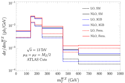
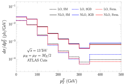
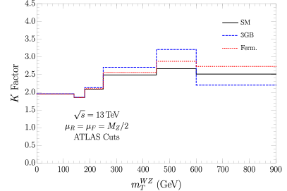
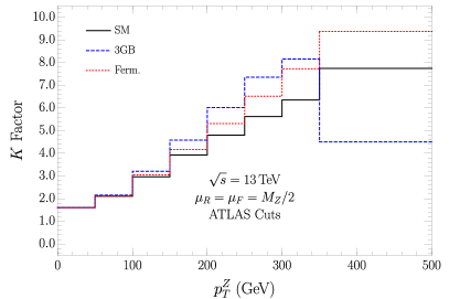
Figure 1: Top Row: Distributions at LO and NLO for the SM, anomalous gauge benchmark point and anomalous fermion benchmark point, Eq. 12, in bins of $m_{T}^{WZ}$ and $p_{T}^{Z}$.
Bottom Row: K-factors for the same three points. In both the $m_{T}^{WZ}$ and $p_{T}^{Z}$ distributions the final bin goes to $2\,\mathrm{TeV}$.

In Fig. 1, we show the distributions in bins of $m_{T}^{WZ}$ and $p_{T}^{Z}$ along with the corresponding ratios of the NLO and LO predictions using the cuts from Ref. Aaboud:2019gxl , where

$$m_{T}^{WZ}=\sqrt{\left(\sum_{\ell=1}^{3}p_{T}^{\ell}+E_{T}^{\mathrm{miss}}\right)^{2}-\left(\sum_{\ell=1}^{3}p_{x}^{\ell}+E_{x}^{\mathrm{miss}}\right)^{2}-\left(\sum_{\ell=1}^{3}p_{y}^{\ell}+E_{y}^{\mathrm{miss}}\right)^{2}}\,.$$ (13)

In the right panel we see that at high $p_{T,Z}$ the $K$ factor for the SM becomes very large as a result of real emission effects that arise at NLO, in agreement with Refs. Denner:2019tmn ; Baglio:2018bkm . In contrast, the $K$ factor grows only modestly as a function of $m_{T}^{WZ}$. For the anomalous coupling benchmarks, we see that the $K$ factor can change quite dramatically, particularly in the higher-momentum bins Baur:1994aj . In the last $p_{T}^{Z}$ bin in particular, the $K$ factor changes from $\sim 7.8$ in the SM to roughly $4.5$ for our “Gauge” benchmark, and $\sim 9.4$ for the “Fermion” point. Similar, but less dramatic, effects are seen in $m_{T}^{WZ}$ as well.

The results of Fig. 1 clearly demonstrate that using the Standard Model $K$ factor in an analysis of anomalous couplings in $WZ$ production is inaccurate at large $p_{T}^{Z}$. As the high transverse momentum bins provide most of the constraining power for fits to the anomalous couplings, this can drastically change the resulting limits on the anomalous coefficients, as we demonstrate in the following sections.

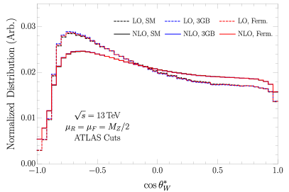
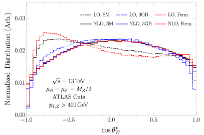
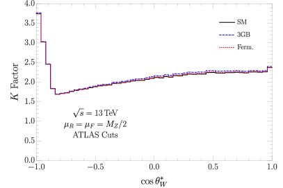
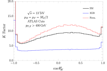
Figure 2: Top Row: Normalized distribution at LO and NLO for the SM, anomalous gauge interaction point and anomalous fermion benchmark points, Eq. 12, in bins of $\cos\theta_{W}^{*}$ with the ATLAS $13\,\mathrm{TeV}$ fiducial cuts Aaboud:2019gxl . The left panel shows the inclusive distribution, while the right panel shows the distribution after an additional cut requiring $p_{T,Z}>400\,\mathrm{GeV}$. Bottom Row: K-factors for the same three points and for the same choice of cuts.

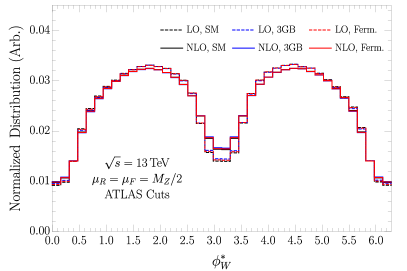
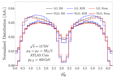
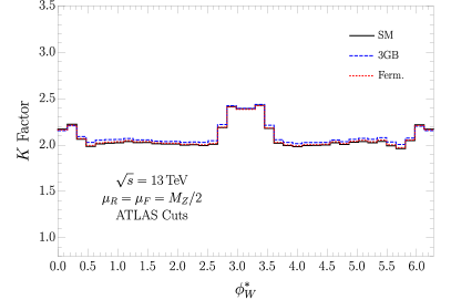
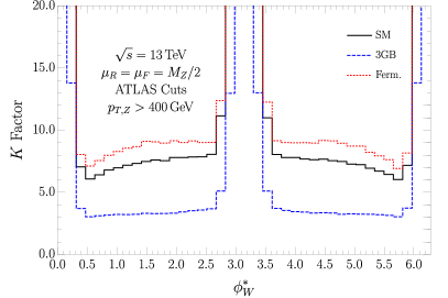
Figure 3: The same as Fig. 2, but for the angular variable $\phi_{W}^{*}$.

We next consider the NLO effects on distributions of the angular variables $\cos\theta^{*}_{W}$ and $\phi^{*}_{W}$. They are the angular variables of the decayed charged lepton in the $W$ rest frame. We use the helicity coordinate system as defined by ATLAS Aaboud:2019gxl , in which the $z$ direction of the $W$ rest frame is the $W$ direction-of-flight as seen in the $WZ$ center-of-mass frame. The definitions of the $x$ and $y$ axes are given in Ref. Bern:2011ie and a graphical representation is given in Ref. Baglio:2018rcu (with a slight modification for the $z$ direction). Angular variables in the decay products (particularly $\cos\theta_{W}^{*}$) are useful for extracting maximal sensitivity to the gauge boson polarizations Panico:2017frx . As emphasized in Refs. Falkowski:2016cxu ; Panico:2017frx ; Franceschini:2017xkh , SMEFT effects lead to quadratic energy growth at the interference level only in the amplitude for producing two longitudinally polarized gauge bosons, Eq. 7. This behavior was exploited in Ref. Franceschini:2017xkh to maximize the sensitivity of the $p_{T,V}$ distribution to anomalous couplings.

In Figs. 2 and 3 we show the normalized distributions of $\cos\theta_{W}^{*}$ and $\phi_{W}^{*}$ for the SM and for our two benchmark points at the fiducial level (left) and with an additional cut requiring $p_{T,Z}>400\,\mathrm{GeV}$ (right) to enhance the sensitivity of the distributions to the anomalous couplings. Without the additional $p_{T,Z}$ cut, the distributions are quite insensitive to the small values of the anomalous couplings in our benchmark points. An interesting effect of the NLO corrections is the washing out of the radiation zero present at LO at $\cos\theta_{W}^{*}=-1$, evidenced by the large $K$ factor in this part of phase space.

After including the $p_{T,Z}$ cut, the LO samples are enriched with longitudinally polarized gauge bosons, and the distributions become much more sensitive to the anomalous couplings. At NLO however, a great deal of this dependence is washed out as a result of the high $p_{T}$ bins being more densely populated due to the real emission present at this order Azatov:2017kzw ; Franceschini:2017xkh . While Ref. Franceschini:2017xkh suggested this could be ameliorated with a jet veto, it was also demonstrated in Ref. Azatov:2017kzw that a hard jet in the process is required to maintain access to the interference terms which grow quadratically with energy and are most sensitive to the SMEFT effects.

IV Fits

The results of Section III demonstrate that including higher-order QCD effects in $WZ$ production in the presence of anomalous gauge and fermion couplings can lead to significantly different predictions than using the LO SMEFT calculation with the Standard Model $K$-factor. We now consider how these effects change the observed limits on the anomalous couplings based on a fit to experimental data. We consider the results in the case of a fit to only $WZ$ data, and then, as a step towards a global analysis, fit both $W^{+}W^{-}$ and $WZ$ data.

The existing experimental results on $W^{+}W^{-}$ and $WZ$ production at both $8$ and $13\,\mathrm{TeV}$ are summarized in Table 1. The $W^{+}W^{-}$ data from ATLAS collected at $8\,\mathrm{TeV}$ in Ref. Aad:2016wpd is systematically lower than the SM prediction in the lower bins, particularly in the 250 – 350 GeV bin. We thus use only the highest bin in $p_{T}^{\mathrm{lead}}$ for our analysis. The $W^{+}W^{-}$ data from CMS at $8\,\mathrm{TeV}$ in Ref. Khachatryan:2015sga includes both same and different flavor final states so there is a contribution from $ZZ$ production that we have not computed, so we do not include this result. The ATLAS $13\,\mathrm{TeV}$ result with $3.16\,\mathrm{fb}^{-1}$ in Ref. Aaboud:2017qkn uses data that is also included in the updated result with $36.1\,\mathrm{fb}^{-1}$ Aaboud:2019nkz , so we will exclude this result as well.

To perform the fits, we construct a $\chi^{2}$ function with the data from the remaining six data sets from Refs. Aaboud:2019nkz ; Aad:2016ett ; Khachatryan:2016poo ; Aaboud:2019gxl ; Sirunyan:2019bez , using the distributions indicated in Table 1. The data in the distributions for Refs. Aaboud:2019nkz ; Aad:2016ett ; Khachatryan:2016poo ; Aaboud:2019gxl , including both statistical and systematic uncertainties was obtained from the corresponding supplementary information. We combine the different sources of uncertainty in quadrature in each bin, neglecting any correlations. The data in Refs. Aad:2016wpd ; Sirunyan:2019bez is not available online, so we digitize the plots to obtain the observed data and statistical uncertainties and add an additional $5\%$ systematic uncertainty bin-by-bin, again neglecting correlations. In each case, the Standard Model prediction for the $W^{+}W^{-}$ or $WZ$ contribution for each distribution was found by digitizing the plots in the experimental papers. To account for detector effects, we normalize our theory predictions bin-by-bin to agree with the Standard Model predictions taken from the experimental results.

Channel	Distribution	# bins	Data set	Int. Lum.
$WW\rightarrow\ell^{+}\ell^{\prime-}+/\!\!\!\!E_{T}\;(0j)$	$p^{\rm leading,lepton}_{T}$, Fig. 11	1	ATLAS 8 TeV	20.3 fb-1 Aad:2016wpd
$WW\rightarrow e^{\pm}\mu^{\mp}+/\!\!\!\!E_{T}\;(0j)$	$p_{T}^{leading,lepton}$, Fig. 7	5	ATLAS 13 TeV	36.1 fb-1 Aaboud:2019nkz
$WZ\rightarrow\ell^{+}\ell^{-}\ell^{(\prime)\pm}$	$m_{T}^{WZ}$, Fig. 5	2	ATLAS 8 TeV	20.3 fb-1 Aad:2016ett
$WZ\rightarrow\ell^{+}\ell^{-}\ell^{(\prime)\pm}+/\!\!\!\!E_{T}$	$Z$ candidate $p_{T}^{\ell\ell}$, Fig. 5	9	CMS 8 TeV	19.6 fb-1 Khachatryan:2016poo
$WZ\rightarrow\ell^{+}\ell^{-}\ell^{(\prime)\pm}$	$m_{T}^{WZ}$ Fig. 4c	6	ATLAS 13 TeV	36.1 fb-1 Aaboud:2019gxl
$WZ\rightarrow\ell^{+}\ell^{-}\ell^{(\prime)\pm}+/\!\!\!\!E_{T}$	$m^{WZ}$, Fig. 15a	3	CMS 13 TeV,	35.9 fb-1 Sirunyan:2019bez

Table 1: Experimental data included in our study. The third column shows the number of bins used in our analysis, always counting from the highest.

IV.1 Fits to $WZ$ Data

We first present the fits to the 8 and $13\,\mathrm{TeV}$ $WZ$ data from ATLAS and CMS Aad:2016ett ; Khachatryan:2016poo ; Aaboud:2019gxl ; Sirunyan:2019bez . In Fig. 4 we show the 95% C.L. allowed regions from various two parameter fits to the anomalous couplings, in each case fixing the other three couplings to zero. As anticipated in Section III, the constraints using the LO and NLO predictions for the SMEFT contributions are quite different. The constraints on the different combinations of gauge couplings are weaker, in some directions by a factor of two. This is consistent with the behavior of the distributions with our “Gauge” benchmark point in Fig. 1. The effect is somewhat less dramatic in the case of anomalous fermion couplings, but there is still a large difference between the limits at LO and NLO.

In Section II.1, we noted that the helicity amplitudes for $WZ$ production had only a sub-leading (in $s/M_{Z}^{2}$) dependence on $\delta\kappa^{Z}$ in the high energy limit. Measurements of $WZ$ production are thus much less sensitive to $\delta\kappa^{Z}$, and we see in Fig. 4 that the limits on $\delta\kappa^{Z}$ are indeed an order of magnitude weaker than those on $\delta g_{1}^{Z}$ and $\lambda^{Z}$. We also note that there is a near flat direction in the $\delta g_{1}^{Z}$ – $\delta g_{L}^{Zu}$ plane, and an even more robust flat direction in the $\delta g_{L}^{Zu}$ – $\delta g_{L}^{Zd}$ plane, in agreement with the scalings in Eq. 7.

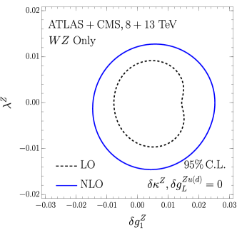
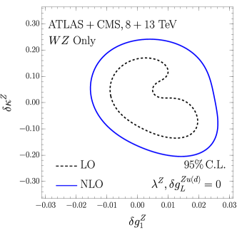
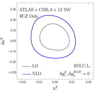
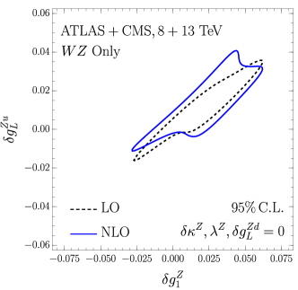
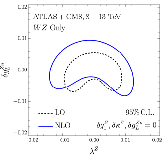
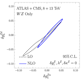
Figure 4: 95% C.L. allowed regions for different combinations of anomalous gauge and fermion couplings based on a fit to the $8$ and $13\,\mathrm{TeV}$ $WZ$ data from ATLAS and CMS Aad:2016ett ; Khachatryan:2016poo ; Aaboud:2019gxl ; Sirunyan:2019bez . The results with the SMEFT treated at leading order (LO) are shown as dashed black contours and the constraints with the SMEFT treated at next-to-leading order (NLO) are shown in solid blue. In each panel we set the three couplings not shown to zero.

IV.2 Combined Fits to $W^{+}W^{-}$ and $WZ$ Data

In the previous section, it was demonstrated that treating the SMEFT consistently at NLO significantly changes the anomalous coupling constraints using $WZ$ data only. On the other hand, in Ref. Baglio:2018bkm , it was shown that the NLO effects on $W^{+}W^{+}$ distributions in the presence of anomalous couplings are relatively mild — in other words, using the $K$-factor derived at the SM is an adequate approximation for setting limits. It is of interest to understand to what extent the significant changes between LO and NLO fits in Fig. 4 remain when including $W^{+}W^{-}$ data. Note that this is only a first step: the anomalous couplings are also constrained by other measurements both in Higgs data, top quark physics and at LEP.

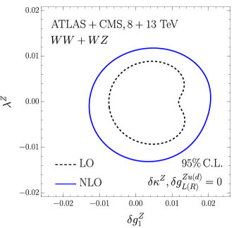
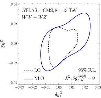
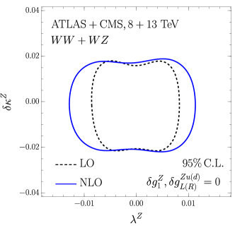
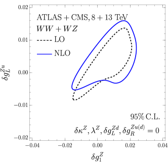
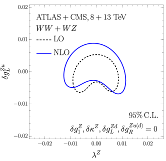
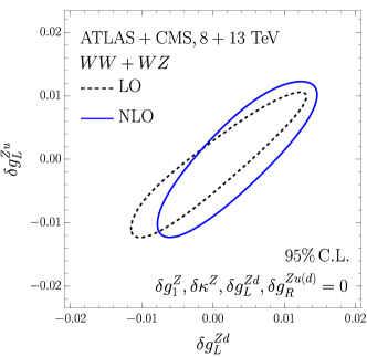
Figure 5: As in Fig. 4, but using both $WW$ and $WZ$ data.

In Fig. 5, we consider the results for various combinations of couplings with the same setup as in Fig. 4, with the other anomalous couplings fixed to zero. The most obvious result is that, even when combined with $W^{+}W^{-}$ data, the effects of treating the SMEFT at NLO in $WZ$ and $W^{+}W^{-}$ production on the limits are still quite substantial in many directions in parameter space. The first panel is clearly mostly constrained by $WZ$ data. As discussed in Subsection IV.1, $\delta\kappa^{Z}$ is much better constrained when $W^{+}W^{-}$ data is included, and since the NLO effects in $W^{+}W^{-}$ production are very small, the limits in the $\delta\kappa^{Z}-\lambda^{Z}$ plane (with all other couplings fixed to zero) are quite similar at LO and NLO. In the $\delta g_{1}^{Z}$ – $\delta\kappa^{Z}$ plane, however, there is a flat direction in $W^{+}W^{-}$ production in the high energy limit (Eq. 8), which is broken by the $WZ$ data and the NLO effects are significant.

We have computed the rates up to quadratic order, $\mathcal{O}(1/\Lambda^{4})$. This has a theoretical complication, however, because in principle dimension-8 operators may contribute at the same order in $1/\Lambda^{4}$ in the most general EFT framework and these effects are not considered here, as we have implicitely assumed that the contributions from the $\mathcal{O}(1/\Lambda^{4})$ dimension-8 operators in the Lagrangian are subleading. We discuss the effects and inherent assumptions involved in truncating the SMEFT expansion explicitly at $\mathcal{O}(1/\Lambda^{2})$, i.e., treating the anomalous couplings only to linear order, in Appendix B. This discussion shows that the $\mathcal{O}(1/\Lambda^{4})$ terms in the cross section are the leading effect in our fits.

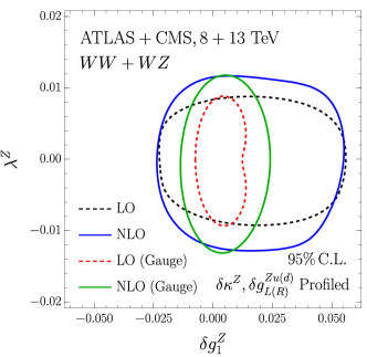
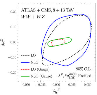
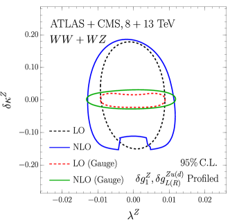
Figure 6: As in Fig. 5, but profiling over the additional operators not shown. The red and green curves show the results profiling only over the gauge couplings at LO and NLO respectively.

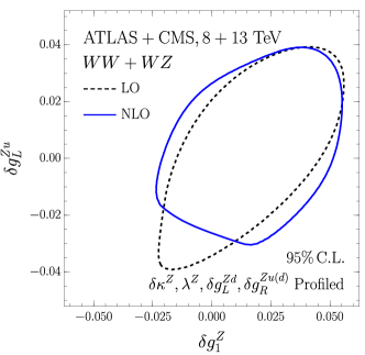
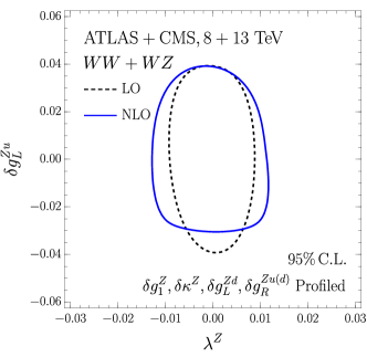
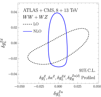
Figure 7: As in Fig. 5, but profiling over the additional operators not shown.

We consider the effects of marginalizing over the operators not shown in each plot. In practice, this is done by minimizing the $\chi^{2}$ function at each point with respect to the other five couplings. In Fig. 6, we show the limits for the three combinations of anomalous gauge couplings, and compare the effects of profiling over the other five anomalous couplings in black (blue) for LO (NLO) with the results when profiling over only the last gauge coupling in red (green) for LO (NLO). In both cases, the effects of considering the anomalous couplings at NLO weaken the bounds on $\lambda^{Z}$. The limits on $\delta g_{1}^{Z}$ in the $\delta g_{1}^{Z}$ – $\delta\kappa^{Z}$ plane are also affected, though the effect is more prominent when profiling only over the gauge couplings. We also see the result, anticipated in Refs. Zhang:2016zsp ; Baglio:2017bfe ; Butter:2016cvz , that the limits on the anomalous gauge couplings are generally much weaker when the fermion couplings are allowed to float within their allowed regions. This is only not true in the $\lambda^{Z}$ direction, as the introduction of $\lambda^{Z}$ leads to a fundamentally different scaling at high energies for the production of transversely polarized $WZ$ (see Eq. 7).

In Fig. 7, we show the constraints in various planes including anomalous fermion couplings, profiling over all five additional parameters. The NLO effects are again apparent, particularly in removing the remaining correlation between $\delta g_{L}^{Zu}$ and $\delta g_{L}^{Zd}$. Finally, we summarize our results in the form of one parameter limits on each of the anomalous couplings considered in Table 2.

Coupling	LO Allowed Range		NLO Allowed Range
	Projected	Profiled	Projected	Profiled
$\delta g_{1}^{Z}$	$~{}[-0.007,\,0.005]~{}$	$~{}[-0.015,\,0.048]~{}$	$~{}[-0.012,\,0.018]~{}$	$~{}[-0.016,\,0.049]~{}$
$\lambda^{Z}$	$~{}[-0.008,\,0.008]~{}$	$~{}[-0.009,\,0.008]~{}$	$~{}[-0.012,\,0.010]~{}$	$~{}[-0.012,\,0.011]~{}$
$\delta\kappa^{Z}$	$~{}[-0.020,\,0.015]~{}$	$~{}[-0.135,\,0.158]~{}$	$~{}[-0.020,\,0.017]~{}$	$~{}[-0.115,\,0.168]~{}$
$\delta g_{L}^{Zu}$	$~{}[-0.002,\,0.005]~{}$	$~{}[-0.034,\,0.034]~{}$	$~{}[-0.001,\,0.008]~{}$	$~{}[-0.022,\,0.035]~{}$
$\delta g_{R}^{Zu}$	$~{}[-0.012,\,0.014]~{}$	$~{}[-0.084,\,0.086]~{}$	$~{}[-0.012,\,0.014]~{}$	$~{}[-0.083,\,0.096]~{}$
$\delta g_{L}^{Zd}$	$~{}[-0.005,\,0.002]~{}$	$~{}[-0.025,\,0.014]~{}$	$~{}[-0.008,\,0.002]~{}$	$~{}[-0.025,\,0.023]~{}$
$\delta g_{R}^{Zd}$	$~{}[-0.018,\,0.017]~{}$	$~{}[-0.045,\,0.048]~{}$	$~{}[-0.018,\,0.017]~{}$	$~{}[-0.053,\,0.043]~{}$

Table 2: $95\%$ C.L. limits on the individual anomalous couplings based on a fit to $W^{+}W^{-}$ and $WZ$ data at LO and NLO, projecting out or profiling over the other couplings.

IV.3 Validity of our Results

The EFT Lagrangian of Eq. 1 is an expansion in powers of (Energy)${}^{2}/\Lambda^{2}$ and so is only valid for energies less than the scale $\Lambda$ Contino:2016jqw ; Farina:2016rws . We consider in Fig. 8 the effects of successively removing the high-energy bins from the single parameter fits to the ATLAS 13 TeV $WZ$ data. If we remove the top bin from the fit, $m_{T}^{WZ}>600$ GeV, then all points in this fit satisfy $m_{T}^{WZ}<\Lambda$ (with $\Lambda=1$ TeV) and the EFT is clearly a valid expansion. In this case, the fit is degraded by ${\cal{O}}(10\%)$ on $\delta\kappa^{Z}$ and ${\cal{O}}(30\%)$ for $\lambda^{Z}$ and $\delta g_{1}^{Z}$, and the NLO QCD effects remain important. It would be interesting to have experimental results where the overflow bin is explicitly separated, so that the maximum energy of the data points in the last bin is clear. The result that interesting limits can be obtained even disregarding the highest-energy bin has been demonstrated using machine learning for the case of $WH$ production in Ref. Brehmer:2019gmn .

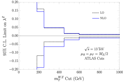
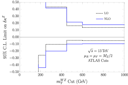
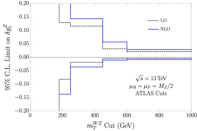
Figure 8: Single parameter fits to ATLAS $13$ TeV WZ data, when successively removing the high $m_{T}^{WZ}$ bins.

V Conclusions

The SMEFT NLO QCD calculation for $pp\rightarrow WZ\rightarrow(l^{\prime}\nu^{\prime})(l^{+}l^{-})$ has been included in the POWHEG-BOX and the primitive cross sections needed to reproduce our results at $8$ and $13$ TeV can be found at https://quark.phy.bnl.gov/Digital_Data_Archive/dawson/wz_19. The NLO QCD effects are significant for $WZ$ production and have an important effect on the global fits to anomalous couplings. The $\mathcal{O}(1/\Lambda^{4})$ terms dominate over the $\mathcal{O}(1/\Lambda^{2})$ terms also when NLO QCD corrections are taken into account. We emphasize again that these results should be interpreted as only a first step in a profiled, global analysis, as all of the couplings — especially the fermionic ones — will be further constrained, and some flat directions removed, by data from LEP and Higgs measurements.

Appendix A Fits to $W^{+}W^{-}$ Production

In this Appendix we present constraints on the anomalous gauge and fermion couplings based on only the $W^{+}W^{-}$ data from ATLAS detailed in Table 1. In Fig. 9, we show the two dimensional limits setting the other anomalous couplings to zero. It is apparent that the NLO QCD effects do not have a significant impact on fits to the $W^{+}W^{-}$ data alone.

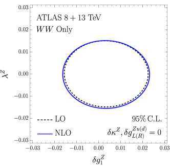
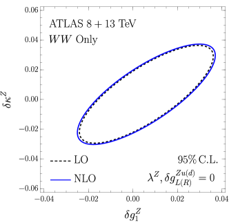
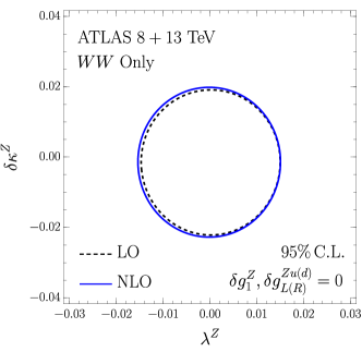
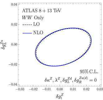
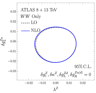
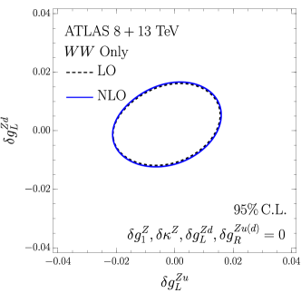
Figure 9: As in Fig. 4, but using only $WW$ data.

Appendix B Truncation to $1/\Lambda^{2}$

If the anomalous couplings are assumed to be small, then the dominant contribution is from the ${\cal{O}}({1/\Lambda^{2}})$ terms which are linear in the anomalous couplings. The results of such a linearized fit are shown in Fig. 10. Since this fit does not include the full amplitude-squared, but just the interference terms it is not guaranteed to be positive definite. The regions with negative cross sections are shaded in grey (blue) for the LO (NLO) predictions, corresponding to regions where the linear approximation is not valid. A comparison of the linear and quadratic fits of Fig. 10 demonstrates that the fits are dominated by the quadratic ${\cal{O}}({1/\Lambda^{4}})$ contributions, and hence the data is not yet sensitive to weak anomalous couplings where the linear approximation would be valid.

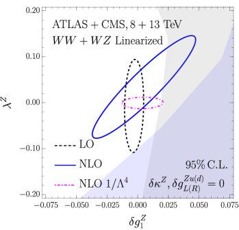
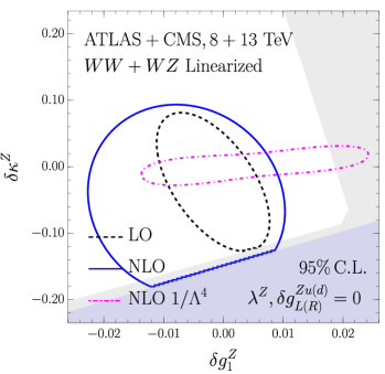
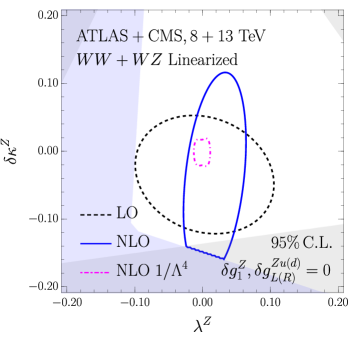
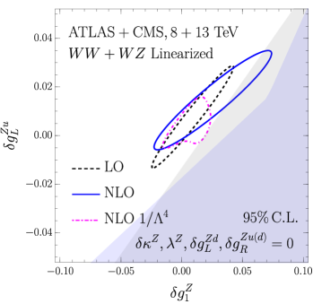
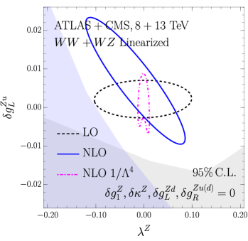
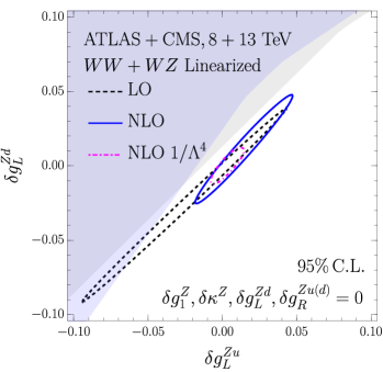
Figure 10: The same as Fig. 5, but keeping only the leading terms in $1/\Lambda^{2}$. Regions where the predicted cross section in any of the bins used for the fit becomes negative are shown in grey (blue for NLO). We include the $1/\Lambda^{4}$ NLO results (pink) for comparison.

References

- (1) S. Dawson, C. Englert, and T. Plehn, “Higgs Physics: It ain’t over till it’s over,” Phys. Rept. 816 (2019) 1–85, arXiv:1808.01324 [hep-ph].
- (2) K. Hagiwara, R. D. Peccei, D. Zeppenfeld, and K. Hikasa, “Probing the Weak Boson Sector in ,” Nucl. Phys. B282 (1987) 253–307.
- (3) Z. Zhang, “Time to Go Beyond Triple-Gauge-Boson-Coupling Interpretation of Pair Production,” Phys. Rev. Lett. 118 no. 1, (2017) 011803, arXiv:1610.01618 [hep-ph].
- (4) J. Ohnemus, “Order- calculation of hadronic z production,” Phys. Rev. D 44 (Dec, 1991) 3477–3489. https://link.aps.org/doi/10.1103/PhysRevD.44.3477.
- (5) S. Frixione, P. Nason, and G. Ridolfi, “Strong corrections to W Z production at hadron colliders,” Nucl. Phys. B383 (1992) 3–44.
- (6) M. Grazzini, S. Kallweit, D. Rathlev, and M. Wiesemann, “ production at hadron colliders in NNLO QCD,” Phys. Lett. B761 (2016) 179–183, arXiv:1604.08576 [hep-ph].
- (7) M. Grazzini, S. Kallweit, D. Rathlev, and M. Wiesemann, “ production at the LHC: fiducial cross sections and distributions in NNLO QCD,” JHEP 05 (2017) 139, arXiv:1703.09065 [hep-ph].
- (8) A. Bierweiler, T. Kasprzik, and J. H. Kuhn, “Vector-boson pair production at the LHC to accuracy,” JHEP 12 (2013) 071, arXiv:1305.5402 [hep-ph].
- (9) J. Baglio, L. D. Ninh, and M. M. Weber, “Massive gauge boson pair production at the LHC: a next-to-leading order story,” Phys. Rev. D88 (2013) 113005, arXiv:1307.4331 [hep-ph]. [Erratum: Phys. Rev.D94,no.9,099902(2016)].
- (10) B. Biedermann, A. Denner, and L. Hofer, “Next-to-leading-order electroweak corrections to the production of three charged leptons plus missing energy at the LHC,” JHEP 10 (2017) 043, arXiv:1708.06938 [hep-ph].
- (11) J. Baglio and N. Le Duc, “Fiducial polarization observables in hadronic WZ production: A next-to-leading order QCD+EW study,” JHEP 04 (2019) 065, arXiv:1810.11034 [hep-ph].
- (12) A. Denner, S. Dittmaier, P. Maierhofer, M. Pellen, and C. Schwan, “QCD and electroweak corrections to WZ scattering at the LHC,” JHEP 06 (2019) 067, arXiv:1904.00882 [hep-ph].
- (13) T. Gehrmann, M. Grazzini, S. Kallweit, P. Maierhofer, A. von Manteuffel, S. Pozzorini, D. Rathlev, and L. Tancredi, “ Production at Hadron Colliders in Next to Next to Leading Order QCD,” Phys. Rev. Lett. 113 no. 21, (2014) 212001, arXiv:1408.5243 [hep-ph].
- (14) F. Caola, K. Melnikov, R. Rontsch, and L. Tancredi, “QCD corrections to production through gluon fusion,” Phys. Lett. B754 (2016) 275–280, arXiv:1511.08617 [hep-ph].
- (15) M. Grazzini, S. Kallweit, S. Pozzorini, D. Rathlev, and M. Wiesemann, “ production at the LHC: fiducial cross sections and distributions in NNLO QCD,” JHEP 08 (2016) 140, arXiv:1605.02716 [hep-ph].
- (16) B. Biedermann, M. Billoni, A. Denner, S. Dittmaier, L. Hofer, B. Jäger, and L. Salfelder, “Next-to-leading-order electroweak corrections to 4 leptons at the LHC,” JHEP 06 (2016) 065, arXiv:1605.03419 [hep-ph].
- (17) W. Buchmuller and D. Wyler, “Effective Lagrangian Analysis of New Interactions and Flavor Conservation,” Nucl. Phys. B268 (1986) 621–653.
- (18) B. Grzadkowski, M. Iskrzynski, M. Misiak, and J. Rosiek, “Dimension-Six Terms in the Standard Model Lagrangian,” JHEP 10 (2010) 085, arXiv:1008.4884 [hep-ph].
- (19) J. Baglio, S. Dawson, and I. M. Lewis, “NLO effects in EFT fits to production at the LHC,” Phys. Rev. D99 no. 3, (2019) 035029, arXiv:1812.00214 [hep-ph].
- (20) L. J. Dixon, Z. Kunszt, and A. Signer, “Helicity amplitudes for O(alpha-s) production of , , , , or pairs at hadron colliders,” Nucl. Phys. B531 (1998) 3–23, arXiv:hep-ph/9803250 [hep-ph].
- (21) L. J. Dixon, Z. Kunszt, and A. Signer, “Vector boson pair production in hadronic collisions at order : Lepton correlations and anomalous couplings,” Phys. Rev. D60 (1999) 114037, arXiv:hep-ph/9907305 [hep-ph].
- (22) U. Baur, T. Han, and J. Ohnemus, “ production at hadron colliders: Effects of nonstandard couplings and QCD corrections,” Phys. Rev. D51 (1995) 3381–3407, arXiv:hep-ph/9410266 [hep-ph].
- (23) A. Azatov, D. Barducci, and E. Venturini, “Precision diboson measurements at hadron colliders,” JHEP 04 (2019) 075, arXiv:1901.04821 [hep-ph].
- (24) T. Melia, P. Nason, R. Rontsch, and G. Zanderighi, “W+W-, WZ and ZZ production in the POWHEG BOX,” JHEP 11 (2011) 078, arXiv:1107.5051 [hep-ph].
- (25) P. Nason and G. Zanderighi, “ , and production in the POWHEG-BOX-V2,” Eur. Phys. J. C74 no. 1, (2014) 2702, arXiv:1311.1365 [hep-ph].
- (26) J. de Blas, M. Ciuchini, E. Franco, S. Mishima, M. Pierini, L. Reina, and L. Silvestrini, “The Global Electroweak and Higgs Fits in the LHC era,” PoS EPS-HEP2017 (2017) 467, arXiv:1710.05402 [hep-ph].
- (27) J. Ellis, C. W. Murphy, V. Sanz, and T. You, “Updated Global SMEFT Fit to Higgs, Diboson and Electroweak Data,” JHEP 06 (2018) 146, arXiv:1803.03252 [hep-ph].
- (28) C. Grojean, M. Montull, and M. Riembau, “Diboson at the LHC vs LEP,” JHEP 03 (2019) 020, arXiv:1810.05149 [hep-ph].
- (29) E. da Silva Almeida, A. Alves, N. Rosa Agostinho, O. J. P. Éboli, and M. C. Gonzalez-Garcia, “Electroweak Sector Under Scrutiny: A Combined Analysis of LHC and Electroweak Precision Data,” Phys. Rev. D99 no. 3, (2019) 033001, arXiv:1812.01009 [hep-ph].
- (30) A. Biekotter, T. Corbett, and T. Plehn, “The Gauge-Higgs Legacy of the LHC Run II,” SciPost Phys. 6 (2019) 064, arXiv:1812.07587 [hep-ph].
- (31) L. Berthier, M. Bjorn, and M. Trott, “Incorporating doubly resonant data in a global fit of SMEFT parameters to lift flat directions,” JHEP 09 (2016) 157, arXiv:1606.06693 [hep-ph].
- (32) S. Dawson and P. P. Giardino, “Electroweak and QCD Corrections to and pole observables in the SMEFT,” arXiv:1909.02000 [hep-ph].
- (33) J. Baglio, S. Dawson, and I. M. Lewis, “An NLO QCD effective field theory analysis of production at the LHC including fermionic operators,” Phys. Rev. D96 no. 7, (2017) 073003, arXiv:1708.03332 [hep-ph].
- (34) N. P. Hartland, F. Maltoni, E. R. Nocera, J. Rojo, E. Slade, E. Vryonidou, and C. Zhang, “A Monte Carlo global analysis of the Standard Model Effective Field Theory: the top quark sector,” JHEP 04 (2019) 100, arXiv:1901.05965 [hep-ph].
- (35) K. J. F. Gaemers and G. J. Gounaris, “Polarization Amplitudes for and ,” Z. Phys. C1 (1979) 259.
- (36) A. Falkowski and F. Riva, “Model-independent precision constraints on dimension-6 operators,” JHEP 02 (2015) 039, arXiv:1411.0669 [hep-ph].
- (37) L. Berthier and M. Trott, “Towards consistent Electroweak Precision Data constraints in the SMEFT,” JHEP 05 (2015) 024, arXiv:1502.02570 [hep-ph].
- (38) U. Baur, T. Han, and J. Ohnemus, “Amplitude zeros in production,” Phys. Rev. Lett. 72 (1994) 3941–3944, arXiv:hep-ph/9403248 [hep-ph].
- (39) R. S. Gupta, A. Pomarol, and F. Riva, “BSM Primary Effects,” Phys. Rev. D91 no. 3, (2015) 035001, arXiv:1405.0181 [hep-ph].
- (40) A. Falkowski, M. Gonzalez-Alonso, A. Greljo, D. Marzocca, and M. Son, “Anomalous Triple Gauge Couplings in the Effective Field Theory Approach at the LHC,” JHEP 02 (2017) 115, arXiv:1609.06312 [hep-ph].
- (41) R. Franceschini, G. Panico, A. Pomarol, F. Riva, and A. Wulzer, “Electroweak Precision Tests in High-Energy Diboson Processes,” JHEP 02 (2018) 111, arXiv:1712.01310 [hep-ph].
- (42) A. Falkowski, M. Gonzalez-Alonso, A. Greljo, D. Marzocca, and M. Son, “Anomalous Triple Gauge Couplings in the Effective Field Theory Approach at the LHC,” JHEP 02 (2017) 115, arXiv:1609.06312 [hep-ph].
- (43) G. F. Giudice, C. Grojean, A. Pomarol, and R. Rattazzi, “The Strongly-Interacting Light Higgs,” JHEP 06 (2007) 045, arXiv:hep-ph/0703164 [hep-ph].
- (44) R. Contino, A. Falkowski, F. Goertz, C. Grojean, and F. Riva, “On the Validity of the Effective Field Theory Approach to SM Precision Tests,” JHEP 07 (2016) 144, arXiv:1604.06444 [hep-ph].
- (45) ATLAS Collaboration, M. Aaboud et al., “Measurement of production cross sections and gauge boson polarisation in collisions at TeV with the ATLAS detector,” Eur. Phys. J. C79 no. 6, (2019) 535, arXiv:1902.05759 [hep-ex].
- (46) Z. Bern et al., “Left-Handed W Bosons at the LHC,” Phys. Rev. D84 (2011) 034008, arXiv:1103.5445 [hep-ph].
- (47) G. Panico, F. Riva, and A. Wulzer, “Diboson Interference Resurrection,” Phys. Lett. B776 (2018) 473–480, arXiv:1708.07823 [hep-ph].
- (48) A. Azatov, J. Elias-Miro, Y. Reyimuaji, and E. Venturini, “Novel measurements of anomalous triple gauge couplings for the LHC,” JHEP 10 (2017) 027, arXiv:1707.08060 [hep-ph].
- (49) ATLAS Collaboration, G. Aad et al., “Measurement of total and differential production cross sections in proton-proton collisions at 8 TeV with the ATLAS detector and limits on anomalous triple-gauge-boson couplings,” JHEP 09 (2016) 029, arXiv:1603.01702 [hep-ex].
- (50) CMS Collaboration, V. Khachatryan et al., “Measurement of the cross section in pp collisions at 8 TeV and limits on anomalous gauge couplings,” Eur. Phys. J. C76 no. 7, (2016) 401, arXiv:1507.03268 [hep-ex].
- (51) ATLAS Collaboration, M. Aaboud et al., “Measurement of the production cross section in collisions at a centre-of-mass energy of = 13 TeV with the ATLAS experiment,” Phys. Lett. B773 (2017) 354–374, arXiv:1702.04519 [hep-ex].
- (52) ATLAS Collaboration, M. Aaboud et al., “Measurement of fiducial and differential production cross-sections at 13 TeV with the ATLAS detector,” arXiv:1905.04242 [hep-ex].
- (53) ATLAS Collaboration, G. Aad et al., “Measurements of production cross sections in collisions at TeV with the ATLAS detector and limits on anomalous gauge boson self-couplings,” Phys. Rev. D93 no. 9, (2016) 092004, arXiv:1603.02151 [hep-ex].
- (54) CMS Collaboration, V. Khachatryan et al., “Measurement of the WZ production cross section in pp collisions at and 8 TeV and search for anomalous triple gauge couplings at ,” Eur. Phys. J. C77 no. 4, (2017) 236, arXiv:1609.05721 [hep-ex].
- (55) CMS Collaboration, A. M. Sirunyan et al., “Measurements of the pp WZ inclusive and differential production cross section and constraints on charged anomalous triple gauge couplings at 13 TeV,” JHEP 04 (2019) 122, arXiv:1901.03428 [hep-ex].
- (56) A. Butter, O. J. P. Eboli, J. Gonzalez-Fraile, M. C. Gonzalez-Garcia, T. Plehn, and M. Rauch, “The Gauge-Higgs Legacy of the LHC Run I,” JHEP 07 (2016) 152, arXiv:1604.03105 [hep-ph].
- (57) M. Farina, G. Panico, D. Pappadopulo, J. T. Ruderman, R. Torre, and A. Wulzer, “Energy helps accuracy: electroweak precision tests at hadron colliders,” Phys. Lett. B772 (2017) 210–215, arXiv:1609.08157 [hep-ph].
- (58) J. Brehmer, S. Dawson, S. Homiller, F. Kling, and T. Plehn, “Benchmarking simplified template cross sections in production,” JHEP 11 (2019) 034, arXiv:1908.06980 [hep-ph].